A Computationally Efficient Moment-Preserving Monte Carlo ...
239
University of New Mexico UNM Digital Repository Nuclear Engineering ETDs Engineering ETDs 6-23-2015 A Computationally Efficient Moment-Preserving Monte Carlo Electron Transport Method with Implementation in Geant4 David Dixon Follow this and additional works at: hps://digitalrepository.unm.edu/ne_etds is Dissertation is brought to you for free and open access by the Engineering ETDs at UNM Digital Repository. It has been accepted for inclusion in Nuclear Engineering ETDs by an authorized administrator of UNM Digital Repository. For more information, please contact [email protected]. Recommended Citation Dixon, David. "A Computationally Efficient Moment-Preserving Monte Carlo Electron Transport Method with Implementation in Geant4." (2015). hps://digitalrepository.unm.edu/ne_etds/12
Transcript of A Computationally Efficient Moment-Preserving Monte Carlo ...
University of New MexicoUNM Digital Repository
Nuclear Engineering ETDs Engineering ETDs
6-23-2015
A Computationally Efficient Moment-PreservingMonte Carlo Electron Transport Method withImplementation in Geant4David Dixon
Follow this and additional works at: https://digitalrepository.unm.edu/ne_etds
This Dissertation is brought to you for free and open access by the Engineering ETDs at UNM Digital Repository. It has been accepted for inclusion inNuclear Engineering ETDs by an authorized administrator of UNM Digital Repository. For more information, please contact [email protected].
Recommended CitationDixon, David. "A Computationally Efficient Moment-Preserving Monte Carlo Electron Transport Method with Implementation inGeant4." (2015). https://digitalrepository.unm.edu/ne_etds/12

David Andrew Dixon
Candidate
Nuclear EngineeringDepartment
This dissertation is approved, and it is acceptable in quality and form for publication:
Approved by the Dissertation Committee:
Prof. Anil Prinja, Chair
Dr. Forrest Brown
Dr. Brian Franke
Dr. Chadwick Lindstrom
Prof. Sean Luan
Prof. Cassiano De Oliviera
i
A Computationally Efficient Moment-PreservingMonte Carlo Electron Transport Method with
Implementation in Geant4
by
David A. Dixon
B.S., Nuclear Engineering, University of New Mexico, 2010
DISSERTATION
Submitted in Partial Fulfillment of the
Requirements for the Degree of
Doctor of Philosophy
Engineering
The University of New Mexico
Albuquerque, New Mexico
May, 2015
ii

Dedication
To my incredible wife, Jessie, and our two wonderful daughters, Maren and
Charlie, a true source of inspiration.
iii

Acknowledgments
Foremost, I would like to thank my advisor, Prof. Anil Prinja, for sharing his ideaswith me, in particular, the Moment-Preserving method. I am truely grateful to havehad such a great mentor and I am hopeful that this is just the beginning of manyexciting and productive collaborations. As a researcher, I can only hope to achievehalf as much as you have during your career and you will always remain as thestandard of excellence that I use to guide myself throughout my career in science.
I would also like to thank my committee members for their participation in thispivotal stage of my life. In particular, I would like to thank Dr. Brian Franke for allof his thoughtful input throughout my experience working on the Moment-Preservingmethod. I should also thank both committee members Dr. Brian Franke and and Dr.Forrest Brown for their support while determining the next step in my career. Theyhave both been instrumental in helping promote my work and myself at both SNLand LANL, and also provided me with some much needed perspective on careers inthe national labs. Finally, I would like to thank the remaining committee membersProf. Sean Luan, Dr. Chadwick Lindstrom, and Prof. Cassiano De Oliveira for theirvaluable input and their patience throughout the entire process.
In addition to my advisor and committee members, I would like to give a specialthanks to friend and mentor Dr. Stan Woolf for setting everything in motion. I wasreally spoiled as a graduate student to get the opportunity to learn from you and itis such a great privilege to have you as a friend.
Lastly, I want to thank my family for your enduring support. None of this wouldhave been possible without you and I will forever remain indebted to you all.
iv

A Computationally Efficient Moment-PreservingMonte Carlo Electron Transport Method with
Implementation in Geant4
by
David A. Dixon
B.S., Nuclear Engineering, University of New Mexico, 2010
Ph.D., Engineering, University of New Mexico, 2015
Abstract
The subject of this dissertation is a moment-preserving Monte Carlo electron trans-
port method that is more efficient than analog or detailed Monte Carlo simulations,
yet provides accuracy that is statistically indistinguishable from the detailed simula-
tion. Moreover, the Moment-Preserving (MP) method is formulated such that it is
distinctly different than Condensed History (CH) methods making the MP method
free of the limitations inherent to CH and proving a viable alternative for trans-
porting electrons. Analog, or detailed, Monte Carlo simulations of charged particle
transport is computationally intensive; thus, it is impractical for routine calcula-
tions. The computational cost of analog Monte Carlo is directly attributed to the
underlying charged particle physics characterized by extremely short mean free paths
(mfp) and highly peaked differential cross sections (DCS). As a result, a variety of
efficient, although approximate solution methods were developed over the past 60
years. The most prolific method is referred to as the Condensed History method.
However, CH is widely known to suffer from inconsistencies between the underlying
v

theory and the application of the method to real, physical problems. Therefore, it
is of interest to develop an alternative method that is both efficient and accurate,
but also a completely different approach to solving the charged particle transport
equation that is free of the limitations inherent to CH. This approach arose from the
development of a variety of reduced order physics (ROP) methods that utilize ap-
proximate representations of the collision operators. The purpose of this dissertation
is the theoretical development and numerical demonstration of an alternative to CH
referred to as the Moment-Preserving method. The MP method poses a transport
equation with reduced order physics models characterized by less-peaked DCS with
longer mfps. Utilizing pre-existing single-scatter algorithms for transporting parti-
cles, a solution to the aforementioned transport equation is obtained efficiently with
analog level accuracy. The process of constructing ROP models and their properties
are presented in detail. A wide variety of theoretical and applied charged particle
transport problems are studied including: calculation of angular distributions and
energy spectra, longitudinal and lateral distributions, energy deposition in one and
two dimensions, a validation of the method for energy deposition and charge de-
position calculations, and response function calculations for full three-dimensional
detailed detector geometries. It is shown that the accuracy of the MP method is
systematically controllable through refinement of the ROP models. In many cases,
efficiency gains of two to three orders of magnitude over analog Monte Carlo are
demonstrated, while maintaining analog level accuracy. That is, solutions gener-
ated sufficient ROP DCS models are statistically indistinguishable from the analog
solution. To maintain analog level accuracy under strict problem conditions, small
efficiency gains are realized. However, loss of efficiency under these conditions is
true of all approximate methods, but the MP method remains accurate where other
methods may fail. That is not to say the MP method does not suffer from limitations
because the MP method will result in discrete artifacts when the problems condi-
tions are strict. However, where limitations of the method arise, they are overcome
vi

through systematic refinement of the ROP DCS models required by the method. In
addition to accuracy and efficiency results, it is shown that the MP method does not
require a boundary crossing or pathlength correction algorithm, which is in great
contrast to the CH method. Finally, implementation and maintenance of the MP
method was found to be straightforward and requires significantly less effort than
CH when measured by the number of lines of code required for each method. In
particular, as compared with the class II CH method utilized in the Geant4 standard
electromagnetic physics list. Ultimately, the MP is shown to be accurate, efficient,
versatile, and simple to implement and maintain.
vii

Contents
List of Figures ix
List of Tables x
1 Introduction 1
2 Literature Review 5
2.1 The Analog Problem . . . . . . . . . . . . . . . . . . . . . . . . . . . 5
2.2 Condensed History . . . . . . . . . . . . . . . . . . . . . . . . . . . . 7
2.3 Reduced Order Physics Models . . . . . . . . . . . . . . . . . . . . . 10
3 Electron Interaction Physics 15
3.1 Nomenclature . . . . . . . . . . . . . . . . . . . . . . . . . . . . . . . 16
3.2 Elastic Collisions with a Nucleus . . . . . . . . . . . . . . . . . . . . 17
3.2.1 Non-relativistic theory . . . . . . . . . . . . . . . . . . . . . . 18
3.2.2 Screened Rutherford and classical Rutherford . . . . . . . . . 19
viii

Contents
3.2.3 Relativistic screened Rutherford . . . . . . . . . . . . . . . . . 21
3.2.4 Partial-wave DCS . . . . . . . . . . . . . . . . . . . . . . . . . 23
3.3 Inelastic Collisions with Atomic Electrons . . . . . . . . . . . . . . . 27
3.3.1 Moller . . . . . . . . . . . . . . . . . . . . . . . . . . . . . . . 27
3.4 Analog DCS Moments . . . . . . . . . . . . . . . . . . . . . . . . . . 29
3.4.1 Elastic DCS moments . . . . . . . . . . . . . . . . . . . . . . 30
3.4.2 Inlastic DCS moments . . . . . . . . . . . . . . . . . . . . . . 33
4 The Analog Problem 36
4.1 Independent Variables . . . . . . . . . . . . . . . . . . . . . . . . . . 37
4.2 The Angular Particle Density and Derived Quantities . . . . . . . . . 38
4.2.1 The angular particle density . . . . . . . . . . . . . . . . . . . 38
4.2.2 Derived quantities . . . . . . . . . . . . . . . . . . . . . . . . 39
4.3 The Electron Transport Equation . . . . . . . . . . . . . . . . . . . . 43
4.4 Analog Monte Carlo Calculations . . . . . . . . . . . . . . . . . . . . 46
4.4.1 Analog Monte Carlo algorithm . . . . . . . . . . . . . . . . . . 46
4.4.2 Tallies . . . . . . . . . . . . . . . . . . . . . . . . . . . . . . . 49
4.4.3 Analog Monte Carlo calculations . . . . . . . . . . . . . . . . 53
5 Differential Cross-Section Moments 65
5.1 Elastic DCS Moments . . . . . . . . . . . . . . . . . . . . . . . . . . 68
ix
Contents
5.2 Inlastic DCS Moments . . . . . . . . . . . . . . . . . . . . . . . . . . 69
5.3 Goudsmit-Saunderson Distribution . . . . . . . . . . . . . . . . . . . 70
5.4 Lewis Theory . . . . . . . . . . . . . . . . . . . . . . . . . . . . . . . 71
5.5 Eigenvalues of the Elastic Collision Operator . . . . . . . . . . . . . . 75
6 The Condensed History Method 78
6.1 The Condensed History Algorithm . . . . . . . . . . . . . . . . . . . 82
6.1.1 Complete grouping, class I . . . . . . . . . . . . . . . . . . . . 83
6.1.2 Mixed procedures, class II . . . . . . . . . . . . . . . . . . . . 85
7 The Moment-Preserving Method 91
7.1 ROP DCS models . . . . . . . . . . . . . . . . . . . . . . . . . . . . . 94
7.2 Derivation of the ROP Collision Operators . . . . . . . . . . . . . . . 96
7.3 Generation of the Discrete and Hybrid Differential Cross-Sections . . 99
7.4 Properties of the ROP Collision Operators and Differential Cross-
Sections . . . . . . . . . . . . . . . . . . . . . . . . . . . . . . . . . . 104
7.4.1 Efficiency: impact of the regularization process . . . . . . . . 105
7.4.2 Accuracy: analog and ROP collision operator eigenvalues . . . 108
8 The Geant4 Toolkit 111
8.1 Developing with the Geant4 toolkit: Application Developers and Toolkit
Developers . . . . . . . . . . . . . . . . . . . . . . . . . . . . . . . . . 112
x

Contents
8.2 The Moment-Preserving Method Classes . . . . . . . . . . . . . . . . 114
8.2.1 Physics processes . . . . . . . . . . . . . . . . . . . . . . . . . 115
8.2.2 Physics models . . . . . . . . . . . . . . . . . . . . . . . . . . 115
8.2.3 Cross-section construction . . . . . . . . . . . . . . . . . . . . 119
8.2.4 Cross section library . . . . . . . . . . . . . . . . . . . . . . . 122
8.2.5 Data processing . . . . . . . . . . . . . . . . . . . . . . . . . . 124
9 Results 127
9.1 Angular Distributions and Energy Spectra . . . . . . . . . . . . . . . 130
9.1.1 Angular distributions . . . . . . . . . . . . . . . . . . . . . . . 131
9.1.2 Energy spectra . . . . . . . . . . . . . . . . . . . . . . . . . . 139
9.1.3 Efficiencies for thin slab problems . . . . . . . . . . . . . . . . 144
9.2 Longitudinal and Lateral Distributions . . . . . . . . . . . . . . . . . 146
9.3 1-D and 2-D Dose Calculations . . . . . . . . . . . . . . . . . . . . . 157
9.3.1 One-dimensional depth-dose profiles . . . . . . . . . . . . . . . 157
9.3.2 Two-dimensional dose deposition . . . . . . . . . . . . . . . . 163
9.4 Comparison with Experiment . . . . . . . . . . . . . . . . . . . . . . 173
9.4.1 Energy deposition profiles . . . . . . . . . . . . . . . . . . . . 173
9.4.2 Charge deposition . . . . . . . . . . . . . . . . . . . . . . . . . 184
9.5 CEASE Response Function Calculation . . . . . . . . . . . . . . . . . 189
xi
Contents
10 Conclusions and Future Work 191
10.1 Conclusions . . . . . . . . . . . . . . . . . . . . . . . . . . . . . . . . 191
10.2 Future Work . . . . . . . . . . . . . . . . . . . . . . . . . . . . . . . . 194
10.2.1 Identification of an analog model . . . . . . . . . . . . . . . . 195
10.2.2 Validation . . . . . . . . . . . . . . . . . . . . . . . . . . . . . 195
10.2.3 Adaptive cross-section selection . . . . . . . . . . . . . . . . . 205
10.2.4 Protons and heavy ions . . . . . . . . . . . . . . . . . . . . . . 206
10.2.5 Variance reduction . . . . . . . . . . . . . . . . . . . . . . . . 206
10.2.6 Deterministic methods . . . . . . . . . . . . . . . . . . . . . . 207
References 208
xii

List of Figures
3.1 Electron interaction diagrams for elastic and inelastic scattering. . . 16
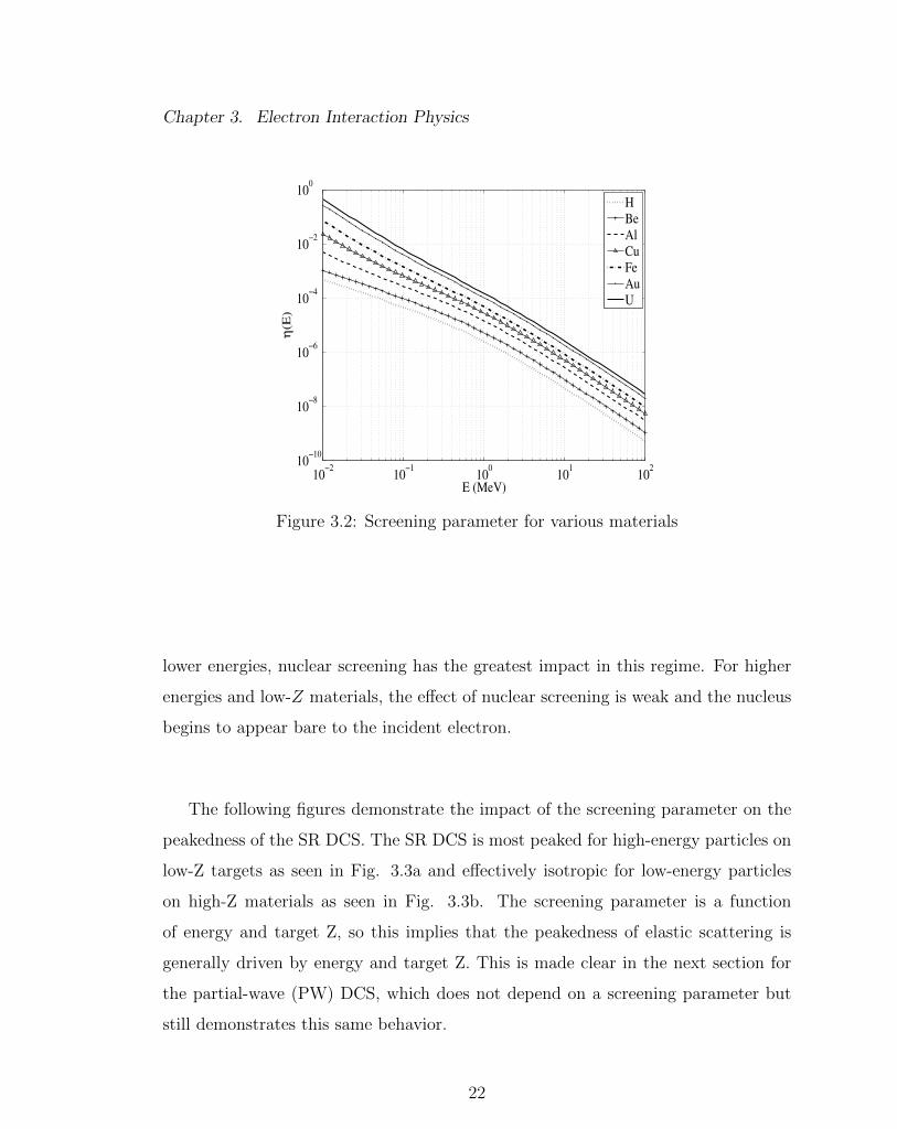
3.2 Screening parameter for various materials . . . . . . . . . . . . . . . 22
3.3 Screened Rutherford (SR) DCS for elastic scattering of 1.026-keV,
1.051-MeV, and 20-MeV electrons by aluminum and gold nuclei. . . 23
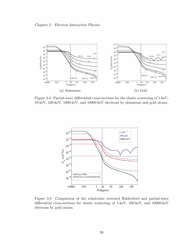
3.4 Partial-wave differential cross-sections for the elastic scattering of
1-keV, 10-keV, 100-keV, 1000-keV, and 10000-keV electrons by alu-
minum and gold atoms. . . . . . . . . . . . . . . . . . . . . . . . . . 26
3.5 Comparison of the relativistic screened Rutherford and partial-wave
differential cross-sections. . . . . . . . . . . . . . . . . . . . . . . . . 26
3.6 Moller inelastic DCS for scattering electrons by aluminum and gold. 28
3.7 Screened Rutherford and partial-wave total cross-sections and mean
free paths for elastic collisions with aluminum and gold nuclei. . . . 32
3.8 Screened Rutherford and partial-wave transport mean free paths for
elastic collisions with aluminum and gold nuclei. . . . . . . . . . . . 33
3.9 Moller total cross-section and mfp for inelastic collisions with alu-
minum and gold nuclei. . . . . . . . . . . . . . . . . . . . . . . . . . 34
xiii
List of Figures
3.10 Comparison of stopping powers. . . . . . . . . . . . . . . . . . . . . 35
4.1 Problem schematic for analog calculation examples. . . . . . . . . . 53
4.2 Reflected and transmitted angular distributions of 1000-keV elec-
trons in aluminum slabs with thickness of 100, 300, 1000, and 3000
analog mfp. . . . . . . . . . . . . . . . . . . . . . . . . . . . . . . . . 55
4.3 Reflected and transmitted angular distributions of 1000-keV elec-
trons in gold slabs with thickness of 100, 300, 1000, and 3000 analog
mfp. . . . . . . . . . . . . . . . . . . . . . . . . . . . . . . . . . . . . 56
4.4 Reflected and transmitted energy-loss spectra for 1000-keV electrons
in aluminum slabs with thickness of 100, 300, 1000, and 3000 analog
mfp. . . . . . . . . . . . . . . . . . . . . . . . . . . . . . . . . . . . . 57
4.5 Reflected and transmitted energy spectra for 1000-keV electrons in
gold slabs with thickness of 100, 300, 1000, and 3000 analog mfp. . . 58
4.6 Longitudinal and lateral distributions of 1000-keV electrons in gold
slabs with thickness of 100, 300, and 1000 analog mfp. . . . . . . . . 58
4.7 Depth-dose profiles for 20000-keV electrons in water and 250-keV
electrons in gold. . . . . . . . . . . . . . . . . . . . . . . . . . . . . . 59
4.8 Charge deposition for 5000-keV and 10000-keV electrons in aluminum
and gold. . . . . . . . . . . . . . . . . . . . . . . . . . . . . . . . . . 60
4.9 Schematic of the CEASE telescope used to measure energy spectra [1]. 62
4.10 CEASE telescope energy threshold matrix with channel labels . . . . 63
4.11 CEASE telescope response function. . . . . . . . . . . . . . . . . . . 64
xiv
List of Figures
5.1 The normal distribution. . . . . . . . . . . . . . . . . . . . . . . . . 66
5.2 Legendre moments and momentum transfer moments of the Partial-
wave differential cross-section for elastic collisions with aluminum
and gold nuclei.. . . . . . . . . . . . . . . . . . . . . . . . . . . . . . 69
5.3 Energy-loss moments of the Moller differential cross-section for in-
elastic collisions with aluminum and gold atomic electrons. . . . . . 70
5.4 Hypothetical paths traveled by electrons. . . . . . . . . . . . . . . . 72
7.1 Comparison of total cross section of screened Rutherford DCS with
several discrete and hybrid DCSs when colliding with gold nuclei. . . 106
7.2 Comparison of total cross section of Moller DCS with several discrete
DCSs when colliding with gold nuclei. . . . . . . . . . . . . . . . . . 106
7.3 Impact of regularization process on reduced order physics DCSs. . . 107
7.4 Comparison of eigenvalues of various approximations of the elastic
collision operator for 1-MeV electrons colliding with gold. . . . . . . 110
9.1 Problem setup for calculation of angular distributions and energy
spectra. . . . . . . . . . . . . . . . . . . . . . . . . . . . . . . . . . . 131
9.2 Transmitted angular distributions for 10000-keV electrons on 100
mfp thick aluminum and gold slabs. . . . . . . . . . . . . . . . . . . 133
9.3 Transmitted angular distributions for 10000-keV electrons on 3000
mfp thick aluminum and gold slabs. . . . . . . . . . . . . . . . . . . 134
9.4 Impact of slab thickness on the transmitted angular distribution for
1000-keV electrons on gold. . . . . . . . . . . . . . . . . . . . . . . . 136
xv

List of Figures
9.5 Impact of aluminum slab thickness on the reflected angular distribu-
tion for 10000-keV electrons on aluminum . . . . . . . . . . . . . . . 137
9.6 Impact of gold slab thickness on the reflected angular distribution
for 1000-keV electrons on gold. . . . . . . . . . . . . . . . . . . . . . 138
9.7 Impact of aluminum slab thickness on the transmitted energy-loss
spectra for 10000-keV electrons . . . . . . . . . . . . . . . . . . . . . 140
9.8 Impact of gold slab thickness on the transmitted energy-loss spectra
for 1000-keV electrons. . . . . . . . . . . . . . . . . . . . . . . . . . 141
9.9 Impact of gold slab thickness on the reflected energy-loss spectra for
10000-keV electrons. . . . . . . . . . . . . . . . . . . . . . . . . . . . 142
9.10 Impact of gold slab thickness on the reflected energy-loss spectra for
1000-keV electrons. . . . . . . . . . . . . . . . . . . . . . . . . . . . 143
9.11 Problem setup for longitudinal and lateral distribution calculations. 147
9.12 Comparison of longitudinal distributions for 10000-keV electrons af-
ter traveling a distance of 100, 300, 1000, and 3000 analog elastic
mfps in copper. . . . . . . . . . . . . . . . . . . . . . . . . . . . . . 151
9.13 Comparison of lateral distributions for 10000-keV electrons after trav-
eling a distance of 100, 300, 1000, and 3000 analog elastic mfps in
copper. . . . . . . . . . . . . . . . . . . . . . . . . . . . . . . . . . . 152
9.14 Comparison of longitudinal distributions for 1000-keV electrons after
traveling a distance of 100, 300, 1000, and 3000 analog elastic mfps
in copper. . . . . . . . . . . . . . . . . . . . . . . . . . . . . . . . . . 153
xvi
List of Figures
9.15 Comparison of lateral distributions for 1000-keV electrons after trav-
eling a distance of 100, 300, 1000, and 3000 analog elastic mfps in
copper. . . . . . . . . . . . . . . . . . . . . . . . . . . . . . . . . . . 154
9.16 Comparison of longitudinal distributions for 100-keV electrons after
traveling a distance of 100, 300, 1000, and 3000 analog elastic mfps
in copper. . . . . . . . . . . . . . . . . . . . . . . . . . . . . . . . . . 155
9.17 Comparison of lateral distributions for 100-keV electrons after trav-
eling a distance of 100, 300, 1000, and 3000 analog elastic mfps in
copper. . . . . . . . . . . . . . . . . . . . . . . . . . . . . . . . . . . 156
9.18 Comparison of depth-dose profiles for 250-keV electrons on gold. . . 158
9.19 Comparison of depth-dose profiles for 20000-keV electrons on water. 160
9.20 Comparison of depth-dose profiles for 150-keV electrons on a gold-
aluminum slab . . . . . . . . . . . . . . . . . . . . . . . . . . . . . . 162
9.21 Problem setup for 150-keV electrons incident on 250-µm by 250-µm
Si cube with gold region . . . . . . . . . . . . . . . . . . . . . . . . . 163
9.22 The relative error in dose from 150-keV electrons in a 250-µm by
250-µm Si/Au cube. . . . . . . . . . . . . . . . . . . . . . . . . . . . 165
9.23 The problem setup and analog benchmark for 10000-keV electrons
on a water/bone cube . . . . . . . . . . . . . . . . . . . . . . . . . . 166
9.24 The relative error in dose from 10000-keV electrons on a water/bone
cube calculated using various discrete models. . . . . . . . . . . . . . 167
9.25 The relative error in dose from 10000-keV electrons on a water/bone
cube calculated using various hybrid models. . . . . . . . . . . . . . 168
xvii
List of Figures
9.26 The schematic of region dependent ROP DCS and the relative error
in dose from 10000-keV electrons on a water/bone cube calculated
using the region dependent ROP DCS with 8-angles applied near the
source and 4-angles applied in all other regions. . . . . . . . . . . . . 170
9.27 The schematic of region dependent ROP DCS and the relative error
in dose from 10000-keV electrons on a water/bone cube calculated
using the region dependent ROP DCS with 8-angles applied in the
peak dose region and 1-angle applied in all other regions. . . . . . . 171
9.28 The problem setup for an isotropic point source located at the origin
of a gold cube (a) and the analog benchmark. . . . . . . . . . . . . . 172
9.29 The relative error in dose from 2500-keV electrons in a gold cube
calculated using various discrete models. . . . . . . . . . . . . . . . . 172
9.30 Comparison with Lockwood data for 1000-keV electrons normally on
carbon slab. . . . . . . . . . . . . . . . . . . . . . . . . . . . . . . . 180
9.31 Comparison with Lockwood data for 500-keV and 1000-keV electrons
normally incident on aluminum slab. . . . . . . . . . . . . . . . . . . 181
9.32 Comparison with Lockwood data for 500-keV and 1000-keV electrons
normally incident on molybdenum slab. . . . . . . . . . . . . . . . . 181
9.33 Comparison with Lockwood data for 500-keV and 1000-keV electrons
normally incident on tantalum slab. . . . . . . . . . . . . . . . . . . 182
9.34 Comparison with Lockwood data for 500-keV electrons with 60 de-
grees off-normal incidence on aluminum slab. . . . . . . . . . . . . . 182
9.35 Comparison with Lockwood data for 500-keV and 1000-keV electrons
with 60 degrees off-normal incidence on molybdenum slab. . . . . . . 183
xviii

List of Figures
9.36 Comparison with Lockwood data for 500-keV and 1000-keV electrons
with 60 degrees off-normal incidence on tantalum slab. . . . . . . . . 183
9.37 Comparison with Tabata data for 5000-keV electrons normally inci-
dent on an aluminum slab. . . . . . . . . . . . . . . . . . . . . . . . 186
9.38 Comparison with Tabata data for 10000-keV electrons normally in-
cident on an aluminum slab. . . . . . . . . . . . . . . . . . . . . . . 186
9.39 Comparison with Tabata data for 20000-keV electrons normally in-
cident on an aluminum slab. . . . . . . . . . . . . . . . . . . . . . . 187
9.40 Comparison with Tabata data for 5000-keV electrons normally inci-
dent on a gold slab. . . . . . . . . . . . . . . . . . . . . . . . . . . . 187
9.41 Comparison with Tabata data for 10000-keV electrons normally in-
cident on a gold slab. . . . . . . . . . . . . . . . . . . . . . . . . . . 188
9.42 Comparison with Tabata data for 20000-keV electrons normally in-
cident on a gold slab. . . . . . . . . . . . . . . . . . . . . . . . . . . 188
9.43 Comparison of response functions. . . . . . . . . . . . . . . . . . . . 190
9.44 Electrons traversing the CEASE telescope. Collimator is in green
and electron tracks are in red. . . . . . . . . . . . . . . . . . . . . . 190
10.1 Comparison of experimental and theoretical energy deposition pro-
files in a tantalum/aluminum configuration for 500 and 1000-keV
electrons normally incident. . . . . . . . . . . . . . . . . . . . . . . . 196
10.2 Comparison of experimental and theoretical energy deposition pro-
files in an aluminum/gold/aluminum configuration for 1000-keV elec-
trons normally incident. . . . . . . . . . . . . . . . . . . . . . . . . . 197
xix

List of Figures
10.3 Energy-deposition distributions of 2-MeV electrons in aluminum and
gold. . . . . . . . . . . . . . . . . . . . . . . . . . . . . . . . . . . . 198
10.4 Energy deposition for 10-MeV and 20-MeV electrons in low-Z and
high-Z materials. . . . . . . . . . . . . . . . . . . . . . . . . . . . . . 198
10.5 Charge-depostion distributions by 5, 10, and 20 MeV electrons inci-
dent on copper and silver . . . . . . . . . . . . . . . . . . . . . . . . 199
10.6 Comparison of experimental and theoretical energy backscatter for
electrons incident at 0 and 60 as a function of target atomic number.200
10.7 Back-scattering coefficient as a function of the mass thickness of alu-
minum films and gold films for different energies normally incident
electrons . . . . . . . . . . . . . . . . . . . . . . . . . . . . . . . . . 201
10.8 Absorption coefficient as a function of the mass thickness of alu-
minum films and gold films for different energies normally incident
electrons . . . . . . . . . . . . . . . . . . . . . . . . . . . . . . . . . 201
10.9 Fano cavity test schematic. . . . . . . . . . . . . . . . . . . . . . . . 202
10.10 Experimental geometry for Ross et al. experiment and differences of
the calculated and measured square characteristic angle. . . . . . . . 204
xx
List of Tables
4.1 Timing results for analog simulation of 106 1-MeV electrons normally
incident on aluminum and gold slabs with varying thicknesses. . . . 54
4.2 Reflection and transmission fractions. . . . . . . . . . . . . . . . . . 61
9.1 Efficiency gains for various ROP DCSs when simulating 1000-keV
and 10000-keV electrons incident on aluminum slabs 100, 300, 1000,
and 3000 mfps thick. . . . . . . . . . . . . . . . . . . . . . . . . . . 145
9.2 Efficiency gains for various ROP DCSs when simulating 1000-keV
and 10000-keV electrons incident on gold slabs 100, 300, 1000, and
3000 mfps thick. . . . . . . . . . . . . . . . . . . . . . . . . . . . . . 145
9.3 Average longitudinal displacement, 〈z〉, for 100-keV, 1000-keV, and
10000-keV electrons in copper after traveling a distance of 100, 300,
1000, and 3000 mfps. . . . . . . . . . . . . . . . . . . . . . . . . . . 149
9.4 Average lateral displacement, 〈x2 + y2〉, for 100-keV, 1000-keV, and
10000-keV electrons in copper after traveling a distance of 100, 300,
1000, and 3000 mfps. . . . . . . . . . . . . . . . . . . . . . . . . . . 149
xxi
List of Tables
9.5 Efficiency gains for various discrete DCSs when calculating dose due
to a beam of electrons with energies of 250-keV, 1000-keV, and 20000-
keV incident on a gold slab. . . . . . . . . . . . . . . . . . . . . . . . 159
9.6 Efficiency gains for various hybrid DCSs when calculating dose due to
a beam of electrons with energies of 250-keV, 1000-keV, and 20000-
keV incident on a gold slab. . . . . . . . . . . . . . . . . . . . . . . . 159
9.7 Speed-up factors for various discrete DCSs when calculating dose
due to a beam of electrons with energies of 250-keV, 1000-keV, and
20000-keV incident on a water slab. . . . . . . . . . . . . . . . . . . 161
9.8 Efficiency gains for various hybrid DCSs when calculating dose due to
a beam of electrons with energies of 250-keV, 1000-keV, and 20000-
keV incident on a water slab. . . . . . . . . . . . . . . . . . . . . . . 161
9.9 Speed-up factors for various discrete DCSs when calculating dose
from 150-keV electrons in a 250-µm by 250-µm Si/Au cube. . . . . . 166
9.10 Speed-up factors for various discrete DCSs when calculating dose
from 10000-keV electrons incident on a 4-cm by 4-cm water cube
with small bone region. . . . . . . . . . . . . . . . . . . . . . . . . . 169
9.11 Total energy deposition comparison for 500-keV and 1000-keV elec-
trons normally incident on aluminum, molybdenum, and tantalum
semi-infinite slabs. . . . . . . . . . . . . . . . . . . . . . . . . . . . . 176
9.12 Total energy deposition for 60 degrees off-normal incidence electrons
on semi-infinite slabs of aluminum, molybdenum, and tantalum. . . 177
9.13 Timing results for energy deposition calculations for 500-keV and
1000-keV electrons normally incident on carbon, aluminum, molyb-
denum, and tantalum semi-infinite slabs. . . . . . . . . . . . . . . . 178
xxii

List of Tables
9.14 Timing results for dose calculations for 60 degrees off-normal inci-
dence electrons on semi-infinite slabs of aluminum, molybdenum, and
tantalum. . . . . . . . . . . . . . . . . . . . . . . . . . . . . . . . . . 179
9.15 Timing results for charge deposition calculations for 5000-keV, 10000-
keV, and 20000-keV electrons normally incident on aluminum and
gold semi-infinite slabs. . . . . . . . . . . . . . . . . . . . . . . . . . 185
xxiii

Chapter 1
Introduction
The need for computational charged particle transport developed from early work in
charged particle transport theory, which emerged as a flourishing subbranch of math-
ematical physics when fast charged particles became available to the experimentalist
[2]. As computer technology improved, the problems of interest to charged particle
computational physicist expanded to areas including:
• Accelerator Physics,
• Medical Physics,
• Health Physics,
• Space Physics,
• Electro-magnetic pulses.
The advantage of computational charged particle transport over analytical transport
is the possibility of simulating complicated geometries and sophisticated boundary
conditions or source configurations, which are all characteristics of real world appli-
cations. In other words, it is possible to simulate real, physical phenomena using
1
Chapter 1. Introduction
charged particle transport codes. An example of such a code is the Geant4 toolkit
[3] which is used frequently on problems including: design of full-scale experiments
such as the Large Hadron Collider [4, 5], design of radiation therapy machines [6] as
well as treatment planning systems [7], estimation of detector geometric factors [8],
shielding calculations [9], and EMP calculations [10]. It is undisputed that particle
transport codes play an important role in the research and development of charged
particle applications and reasonable to suggest that particle transport codes will con-
tinue to play an important role into future. Therefore, algorithmic improvements to
particle transport codes are critical to improving the field of computational charged
particle transport.
To make clear the impact of this work and the importance of the remaining chap-
ters, it is necessary to provide, at least, a cursory discussion on what is meant by
charged particle transport codes and the associated challenges. First, the purpose
of charged particle transport codes is to obtain solutions to the Boltzmann trans-
port equation [11] using stochastic methods like Monte Carlo [12] or deterministic
methods like SN [13]. The Boltzmann transport equation is a balance equation for
particles in a six-dimensional phase-space including space, angle, and energy. The
solution to this equation describes the particle population and is referred to as the
angular flux. For a given analog DCS model, the corresponding transport equation is
referred to as the analog model and the angular flux is assumed to be exact. Analog,
(detailed, step by step), simulation is feasible under strict circumstances (relatively
low energies, thin targets,...), but for high-energy electrons (above a few hundred
keV), the number of interactions suffered by an electron along its trajectory is too
large for detailed simulations [14]. For this reason, numerous computationally effi-
cient approximate methods have emerged over the past 60 years. The most notable
and prolific approximate method is Condensed History (CH). Berger describes CH
as an (artificially constructed) random walk, each step of which takes into account
the combined effects of many collisions [2]. The distances between collisions or the
2

Chapter 1. Introduction
steps are significantly longer than those associated with the analog problem, mak-
ing CH efficient. However, the theoretical basis and practical implementation of the
CH algorithm introduces inherent and irreducible limitations that are unique to the
method [15].
It is of interest to develop a method free of such limitations. That is, an efficient
moment-preserving method for Monte Carlo electron transport, which is the subject
of this dissertation. The central question addressed herein is whether the efficiency
and accuracy associated with the Moment-Preserving (MP) method are sufficient to
recommend this method as an alternative to the CH method. This is addressed in
two ways. First, theoretical development of the method is discussed in great detail
to emphasize how elements of accuracy and efficiency are inherent to the method.
The theoretical development is followed up with an extensive numerical demonstra-
tion of the method including calculations of angular distributions, energy spectra,
lateral and longitudinal distributions, one-dimension and two-dimension dose de-
position, one-dimension charge deposition, and a multi-dimensional space physics
application. In addition, specific results are presented that demonstrate how the
moment-preserving method is free from the limitations inherent to CH. State-of-
the-art tabulated elastic DCSs generated using the ELSEPA code system were used
to demonstrate the versatility of the method. Finally, all of the algorithmic devel-
opment was completed within the Geant4 toolkit [3] to demonstrate the simplicity
of the method from a code implementation and maintenance standpoint. Through
demonstration of the accuracy, efficiency, versatility, and simplicity of the method,
the question central to this dissertation is addressed.
The remainder of the dissertation provides the background information necessary
to understand the results, a discussion of the Geant4 toolkit and implementation de-
tails specific to the MP method, results, conclusions, and future work. The remaining
chapters are organized as follows:
3

Chapter 1. Introduction
• Chapter 2: Literature Review
• Chapter 3: Electron Interaction Physics
• Chapter 4: The Analog Problem
• Chapter 5: Differential Cross-Section Moments
• Chapter 6: The Condensed History Method
• Chapter 7: The Moment-Preserving Method)
• Chapter 8: The Geant4 Toolkit
• Chapter 9: Results
• Chapter 10: Conclusions and Future Work
4

Chapter 2
Literature Review
This chapter provides a qualitative discussion of the literature relevant to the ana-
log problem and the associated analog differential cross-sections (DCS) (detailed in
chapter 3 and chapter 4), the Condensed History (CH) method (detailed in chapter
6), and the Moment-Preserving (MP) method (detailed in chapter 7). The analog
problem is the point of departure for both CH and ROP models, so we begin with a
discussion of the analog problem.
2.1 The Analog Problem
The analog description of transport can be mathematically expressed in terms of
the linear Boltzmann or transport equation for the angular flux, where the inter-
action physics are represented through total cross sections (inverse mfp) and the
DCSs for angular deflection and energy loss [15]. The total cross sections and DCSs
appear in the elastic and inelastic collision operators, which are integral operators
or Boltzmann-type operators. Though electrons can undergo several different elec-
5

Chapter 2. Literature Review
tromagnetic interactions1, the dominant interactions are elastic collisions with nu-
clei and inelastic collisions with atomic electrons. Typical DCSs for elastic nuclear
scattering include relativistic screened Rutherford, Wentzel, or the partial-wave ex-
pansion [16, 17, 18], while typical DCSs for inelastic electronic scattering include
Rutherford, Moller, or the Evaluated Electron Data Library [19, 20]. These DCSs
are highly peaked about small changes in direction and small energy losses and the
associated total cross sections are very large resulting in extremely short mfps. In-
teraction physics of this nature present a difficult computational task.
Boundary conditions for the transport equation depend on the application, but
typically include vacuum, pencil beams, or sources distributed in space, energy, and
angle. However, mono-energetic pencil beams are very common in electron trans-
port and further complicate the computational challenges because pencil beams are
singular in space, energy, and angle.
The problem of computational inefficiencies associated with the analog physics
was recognized immediately by early charged particle computational physicists. In
fact, Berger [2] acknowledged that a direct analog Monte Carlo procedure would be
quite costly, because of the enormous number of collisions that must be sampled.
For example, it takes on the order of tens of thousands of collisions for an electron
with energy of roughly 1-MeV to slow down to 1-keV, while only 20 to 30 Compton
scatterings will reduce the energy of a photon from several MeV down to 1-keV
or 18 elastic collisions in hydrogen will reduce a neutron from 2-MeV to thermal
energies [2]. In 1963, only one calculation by direct analog Monte Carlo was reported
[21]. Since then, several analog Monte Carlo electron transport codes have been
developed [14, 22] and a few production codes have included analog physics options
[23, 24, 25]. Solutions to the analog problem are exact for a given DCS; therefore,
1Bremsstrahlung is an important interaction for relativistic electrons. However, bremsstrahlungdoes is not a computationally intensive process, so it is neglected in this work. It should be notedthat use of preexisting bremsstrahlung physics with the moment-preserving method will not impactthe efficacy of the method.
6
Chapter 2. Literature Review
it is understandable that analog physics options were implemented, despite the fact
that analog Monte Carlo is computationally inefficient. Moreover, it is feasible to use
analog Monte Carlo for occasional calculations if significant computing resources are
available. However, analog Monte Carlo remains impractical for routine calculations
with exception of very restrictive problems like transport through optically thin
materials. For this reason, approximate methods remain a critical component of
most Monte Carlo electron transport codes.
2.2 Condensed History
Condensed history has been the prevailing approximate method in computational
charged particle transport since the emergence of the field. The usual practice is to
use “condensed” (class I) simulation methods, in which the global effect of multi-
ple interactions is described by means of approximate multiple scattering theories.
Alternatively, one can use “mixed” (class II) schemes in which hard (catastrophic)
interactions, with energy loss or angular deflection above given thresholds, are sim-
ulated individually. For a given set of DCSs, class II schemes are intrinsically more
accurate than class I simulations [14]. Some examples of codes containing class
I schemes are ETRAN, ITS, MCNP, while examples of production codes contain-
ing class II CH schemes are EGS4, PENELOPE, Geant4 [26, 27, 3]. Both class I
and class II schemes utilize various results from multiple scattering theory, which
is a subbranch of mathematical physics developed around the solution of the trans-
port equation with limited applicability resulting from severe restrictions required
to obtain analytical solutions [28, 29, 30, 31]. The analytical solutions or multiple
scattering distributions describe the angular or energy distributions of electrons after
traveling some distance s or a step, that are on the order of hundreds of analog mfps.
The major distinction between class I and class II schemes is how the grouping of
7
Chapter 2. Literature Review
collisions is handled. That is, class I schemes utilize precomputed multiple-scattering
(MS) distributions [32, 33, 34, 35] determined for fixed step-sizes on a fixed energy
grid. For this reason, energy straggling is sampled from a MS distribution [34, 35]
and secondaries are accounted for on an average basis. Therefore, it is not possible to
distinguish between inelastic collisions resulting in secondary production (hard) and
those that do not (soft). In contrast, a class II scheme like EGS allows all physical
processes and boundaries to affect the choice of step size [36]. Thus, distance to hard
collision is exponentially distributed and secondary production is treated exactly
by sampling energy-loss from the inelastic DCS above the secondary production
threshold.
Regardless of the choice in the scheme, substantial efficiency gains over analog
Monte Carlo can be realized with CH. However, the accuracy of early forms of CH
was strongly dependent on step-size and while it was found that reducing the elec-
tron step-size causes the results to converge to the correct values, the computing time
increases rapidly in proportion to the inverse of the step-size [37, 38, 39]. Therefore,
special algorithms like PRESTA [40] were developed to select the optimal step-size
during the process of a Monte Carlo simulation. Without an algorithm like PRESTA,
one must resort to a tedious study to determine the optimal step-size such that ac-
ceptable accuracy and efficiency is achieved. However, this optimization may not be
universal. The various production codes currently available differ in this optimization
issue. Some codes, like ITS, have pre-determined step-size parameters, while codes
like EGS utilize the PRESTA algorithm [40] or random hinging combined with lat-
eral corrections found in PENELOPE. In addition to step-size limitations, condensed
history suffers from inconsistent handling of the material and free surface boundaries.
Material interfaces are a fundamental challenge for condensed history because the
MS distributions are infinite medium solutions and are not valid for heterogenous
regions. Therefore, if a material interface is encountered, a special algorithm like the
Jordan-Mack algorithm [41] or PRESTA is required. Another issue specific to class
8

Chapter 2. Literature Review
I schemes that utilize the Goudsmit-Saunderson distribution [32, 33] for sampling
angular deflection is that the numerical methods required to generate the Goudsmit-
Saunderson distribution are sensitive to small step-sizes. The backwards recurrence
used to generate the Goudsmit-Saunderson is unstable for small steps. Even if the
step-size is sufficiently long that the backwards recurrence is stable, it is possible
that more than the pre-scripted number of recurrence coefficients are required to
accurately resolve the Goudsmit-Saunderson distribution [42].
There are many forms of MS theory that are fundamental to CH, but one of
particular importance to all approximate methods is referred to as Lewis theory [43].
A concise description of Lewis theory is given by Prinja [44]:
Consider an infinite medium in which charged particles undergo scatter-
ing collisions resulting in angular deflection but no energy losses. Let the
differential scattering cross section be given by Σ(A)s (~Ω′ ·~Ω) with ~Ω′ and ~Ω
being pre- and post-collision unit direction vectors and where the label A
denotes a specific configuration of this problem. The Legendre moments
of this cross-section are defined by Σ(A)s,n =
∫4π
Σ(A)s (~Ω · ~Ω′)Pn(~Ω · ~Ω′)d2Ω,
where Pn(µ), −1 ≤ µ ≤ 1, are the Legendre polynomials. The cross-
section or its associated moments and the charged particle source com-
pletely characterize this problem. Consider now, a second configuration,
labeled B, that is characterized by the same source but a different differ-
ential scattering cross-section Σ(B)s (~Ω′ · ~Ω) and hence different moments
Σ(B)s,n . In general, the particle angular distributions or angular fluxes for
the two problems, ψA,B(~r, ~Ω), will be different. However, if the cross-
sections are related such that Σ(A)s,n = Σ
(B)s,n , n = 1, 2, ...N, for some fixed
order N and Σ(A)s,n 6= Σ
(B)s,n , n ≥ N + 1,then a classic result due to Lewis
[43] states that space-angle moments of the two angular fluxes defined
by Mmx,my ,mzj,k,l =
∫V
∫|~Ω|=1
xjykzlΩmxx Ω
myy Ωmz
z ψA,B(~r, ~Ω)d2ΩdV and com-
9
Chapter 2. Literature Review
monly referred to as Lewis-moments, are identical through any order
satisfying j + k + l + mx + my + mz = N , where (Ωx,Ωy,Ωz) are the
direction cosines with respect to the Cartesian axes (x, y, z).
The significance of this observation is that if Σ(A)s (~Ω′ · ~Ω) is the true
or exact differential cross-section for scattering of the charged particle
by the target nucleus, also referred to as the analog differential cross-
section, and Σ(B)s (~Ω′ · ~Ω) is an approximation to it, Lewis’ result points to
a sharp link between accuracy of the approximate model, as measure by
linear functionals (moments) of the angular flux, and number of Legendre
moments of the differential cross-section that are exactly reproduced in
the approximate model.
2.3 Reduced Order Physics Models
For the reasons stated above, various alternatives to the CH method were developed.
Of particular interest are alternatives referred to as Reduced Order Physics (ROP)
models, which are a family of transport-based approximations. ROP models include
various approximate representations of the analog collision operators that are of both
integral and differential forms. ROP models are obtained through some type of reg-
ularization procedure that removes reduce the nearly-singular behavior of the analog
DCS, while systematically capturing the key physics through preservation of angu-
lar and energy-loss moments of the analog DCSs. Moreover, the zeroth or the total
cross section is not preserved, rather it is determined self-consistently by the method.
The resulting ROP model is then characterized by less peaked scattering with mfps
longer than the analog mfp. Efficiency is achieved by not preserving the total cross
section, while accuracy is achieved by preserving the necessary number of moments
beyond the zeroth. There are numerous approximations that qualify as ROP models
10
Chapter 2. Literature Review
including Fokker-Planck, Boltzmann Fokker-Planck, Generalized Fokker-Planck, and
Generalized Boltzmann Fokker-Planck. The remainder of this chapter is devoted to
introducing each of these approximations and indicating how these methods con-
tributed to the development of the MP method.
The classical Fokker-Planck operator is obtained by Taylor expanding the scatter-
ing kernels. This is a reasonable approach, assuming the angular flux is sufficiently
smooth, because the DCSs fall off rapidly away from small deflection cosines and
energy-losses. The resulting operator is differential in angle and energy and models
elastic and inelastic scattering as diffusive processes. As a result, the Fokker-Planck
operator does not capture large-angle scatter and can lead to energy gains. Pom-
raning confirmed these inconsistencies by showing that the Fokker-Planck operator
is an asymptotic limit of the Boltzmann collision operator and only valid for unre-
alistically peaked scattering [45]. That is, the FP approximation is strictly valid in
the limit that the total scattering cross section goes to infinity and the mean deflec-
tion cosine goes to unity such that the transport cross section remains bounded [46].
Under these conditions, large angle scattering is negligible and the FP operator is
equivalent to the Boltzmann integral collision operator. Clearly, there is a limita-
tion on the type of physics for which the classical FP operator is valid. Regardless,
various implementations of Fokker-Planck operator were studied for in deterministic
settings[47, 48, 49, 50].
In efforts to incorporate large-angle scattering, a kernel decomposition approach
was introduced by Ligou and is referred to as the Boltzmann-Fokker-Planck (BFP)
equation [51, 52, 53]. Ligou recognized that it is easier to numerically treat forward-
peaked elastic scattering and small energy losses associated with such scattering
using Fokker-Planck (FP) differential operators [49] rather than Boltzmann integral
operators. However, the FP operator does not accurately capture large angle scat-
tering. Therefore, it is necessary to decompose the scattering cross section into its
11
Chapter 2. Literature Review
singular and smooth components and apply the FP approximation to the singular
component while leaving the smooth operator intact [54]. One important feature of
the decomposition process is that there is no rigorous definition of the components
so there are infinite decompositions. The key, as indicated by Landesman and Morel
[54], is to select a decomposition that is not only accurate and efficient, but also
easily integrated into existing transport codes. The early methods for solving the
BFP equation were deterministic, but Morel and Sloan [55, 56] developed a hybrid
multigroup/continuous-energy Monte Carlo method for solving the BFP equation or
the MGBFP method. Morel described the MGBFP method as a new form of con-
densed history with the major distinction being that path lengths between collision
sites are exponentially distributed.
In retrospect, application of kernel decomposition serves to stabilize the diver-
gent behavior of the Fokker-Planck expansion [57] by effectively renormalizing the
expansion coefficients. This renormalization process is central to the Generalized
Fokker-Planck (GFP) method [58, 59] and resulted after attempting to generalize
the FP operator to a broad class of physics with higher order FP operators [57]. In
principle, the FP approximation can be improved by retaining higher order terms
in the Taylor expansion of the collision operators. Thus, leading to a more accurate
description of large angle scattering, but this is only true for specific kernels. For
example, it is known that there are no valid FP operators for the Henyey-Greenstein
kernel [45] and that the standard FP operator is only marginally valid for screened
Rutherford or screened Mott [46]. However, Pomraning [57] completed the same
kernel analysis for the exponential and delta function and showed that higher order
FP operators are valid for kernels such as these, but they are unphysical. In addition
to characterizing the stability of higher order FP operators with respect to specific
scattering kernels, this analysis revealed the explicit role of the analog DCS moments
to developing approximations. That is, higher order FP expansions suggest that the
accuracy of the approximation is improved by incorporating higher order moments.
12
Chapter 2. Literature Review
GFP approaches provide a means to stabilize higher-order FP operators through
renormalization of the various terms that appear in the operator. The renormal-
ization process, in essence, allows for an arbitrary ordered FP operator; hence, the
approach referred to as generalized FP. Lastly, work on GFP showed that the key
to a stable ROP model is preserving the integral form of the collision operator and
retaining an arbitrary number of low order moments while approximating all of the
higher order moments.
Insight gained from the foregoing approximations - FP, BFP, and GFP - com-
bined with Lewis theory and practical experience from implementing and testing
CH led to the development of the Generalized Boltzmann Fokker-Planck (GBFP)
method [60]. Like the other ROP models, the GBFP method is a transport-based
approximation. However, the GBFP method is more appropriate for Monte Carlo
calculations like CH. The emphasis of GBFP method is the development of stable,
moment-preserving representations of the collision operators. This is achieved by
constructing ROP DCSs that are moment-preserving, per Lewis theory, while leav-
ing the collision operators intact by simply replacing the analog DCSs with the ROP
DCSs. Another key feature of the GBFP approach is that angular deflection and
energy-loss interactions depend only on Legendre moments and energy-loss moments,
not the detailed form of the analog DCSs. Therefore, the GBFP method is applicable
to both continuous DCSs [61] and tabulated DCS data [62] and code modifications
are not required for physics refinements because this is accomplished by providing
moments of the desirable analog model through input data. The bulk of the work
on the GBFP method to date emphasizes the most simple, but also the most effec-
tive ROP DCSs referred to as the discrete and hybrid models. The discrete model
[63] is a superposition of discrete points and weights over the full range of the DCS,
while the hybrid model [64] is a superposition of discrete points and weights over the
peaked portion of the DCS and the tail is represented exactly by the analog DCS.
Recently, the name Moment-Preserving method was adopted in place of the GBFP
13

Chapter 2. Literature Review
method to distinguish the method from Fokker-Planck and to emphasize the concept
most fundamental to the method - moment preservation.
14

Chapter 3
Electron Interaction Physics
In this chapter, interactions of electrons are detailed. Differential cross-sections
(DCS) appropriate for moderate to high energies above roughly 10-keV are con-
sidered. At these energies, electrons are treated as point particles where they are
assumed free streaming between collisions. The medium is assumed amorphous and
for a single element with atomic number Z and density ρ the material properties
are given by the number density N . The extension to compounds, and mixtures, is
normally done on the basis of the additivity approximation, i.e., the molecular DCS
is approximated as an incoherent sum of the atomic DCSs of all of the atoms in
a molecule [27]. Electron interactions include elastic scattering with atomic nuclei,
inelastic scattering with atomic electrons, bremsstrahlung emission, and elastic col-
lisions with atomic electrons. However, the subject of this work is the treatment of
Coulomb collisions that contribute significantly to the computational inefficiencies
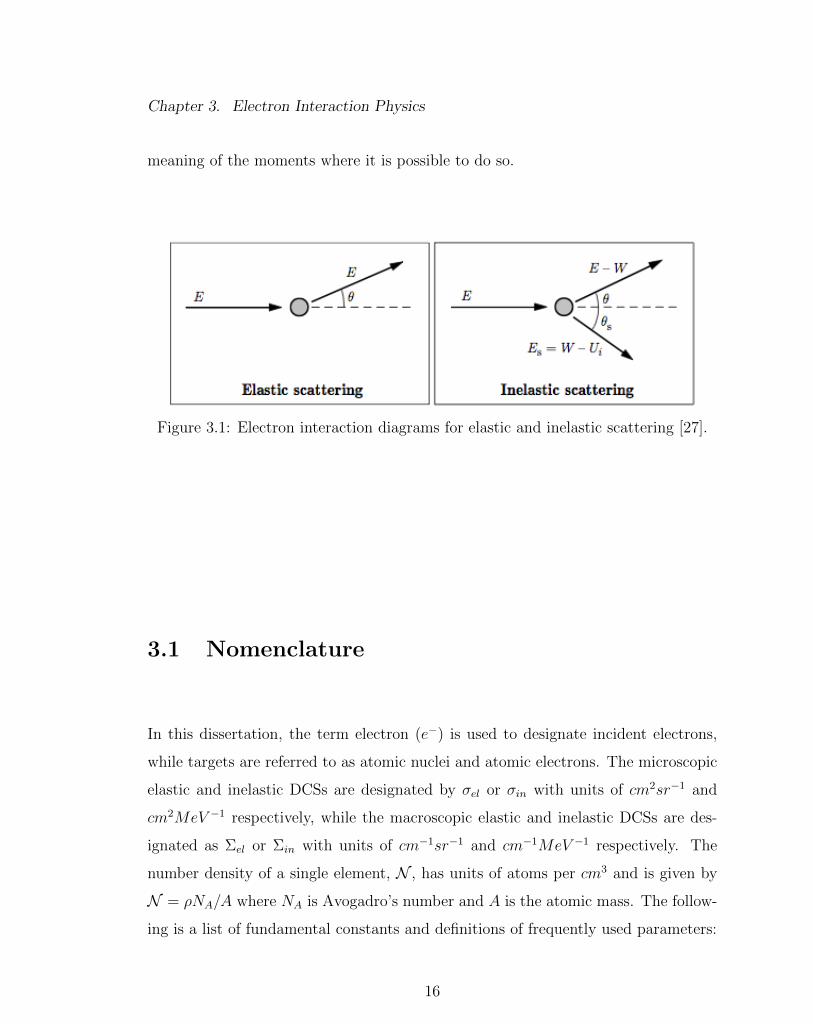
associated with analog transport (specifically, elastic and inelastic collisions as in
Fig. 3.1). The analog elastic and inelastic DCSs utilized in this work include analyt-
ical functions and tabulated DCS data and are described in the following sections.
Moments of analog DCSs are central to the moment-preserving method, so the last
section defines the elastic and inelastic DCS moments and discusses the physical
15
Chapter 3. Electron Interaction Physics
meaning of the moments where it is possible to do so.
Figure 3.1: Electron interaction diagrams for elastic and inelastic scattering [27].
3.1 Nomenclature
In this dissertation, the term electron (e−) is used to designate incident electrons,
while targets are referred to as atomic nuclei and atomic electrons. The microscopic
elastic and inelastic DCSs are designated by σel or σin with units of cm2sr−1 and
cm2MeV −1 respectively, while the macroscopic elastic and inelastic DCSs are des-
ignated as Σel or Σin with units of cm−1sr−1 and cm−1MeV −1 respectively. The
number density of a single element, N , has units of atoms per cm3 and is given by
N = ρNA/A where NA is Avogadro’s number and A is the atomic mass. The follow-
ing is a list of fundamental constants and definitions of frequently used parameters:
16

Chapter 3. Electron Interaction Physics
Speed of Light c = 2.99792458× 10⁸ m/s
Reduced Planck’s Constant h = 6.58211928× 10⁻¹⁶ eV· s
Electron Rest Mass mec2 = 0.510998910 MeV
Classical Electron Radius r0 = 2.8179403267× 10⁻¹³ cm2
Avogadro’s Number NA = 6.0221413× 10²³ atoms/mole
Energy Per Rest Mass τ = E/mec2 (unitless)
Lorentz Factor γ = 1 + τ (unitless)
Ratio of Electron Velocity to c β =√
1− 1/γ2 (unitless)
3.2 Elastic Collisions with a Nucleus
The basic quantity describing the elastic scattering of electrons by a target system is
the elastic DCS that can be accurately described by a static central potential V (r).
Given an idealized scattering experiment where a mono-directional, mono-energetic
beam of electrons with a current ~jinc of electrons passing through a surface area
per unit time are scattered through some differential solid angle dΩ into a detector
measuring counts per unit time Ncount, the microscopic elastic DCS is defined as
σel ≡Ncount
|~jinc|dΩ. (3.1)
Though the DCS can be determined experimentally, accurate theoretical expressions
for the count rate and the current can be derived. A comprehensive review of such
theoretical expressions is described in great detail in the ICRU Report 77 [65]. How-
ever, some attention is given to the theoretical development of the DCSs that are
utilized in this dissertation.
Herein, incident electrons in the regime of kinetic energies higher than ≈ 10-keV
are considered, where the interaction with the target atom is likely sudden, i.e., the
interaction time is so small that the atomic electron cloud is not appreciably distorted
by the interaction [65]. Under these conditions, the target atom is considered a
17
Chapter 3. Electron Interaction Physics
frozen distribution of electric charge (static-field approximation) and treated as a
point nucleus. Elastic scattering is then assumed to be the scattering of the incident
electron by the electric field of the atom. The electric field of an atom is assumed
spherical and therefore it is a good approximation to assume the interaction potential
V (r) depends only on the distance r between the incident electron and the nucleus
of the atom. Given these assumptions several forms of the elastic DCS are reviewed.
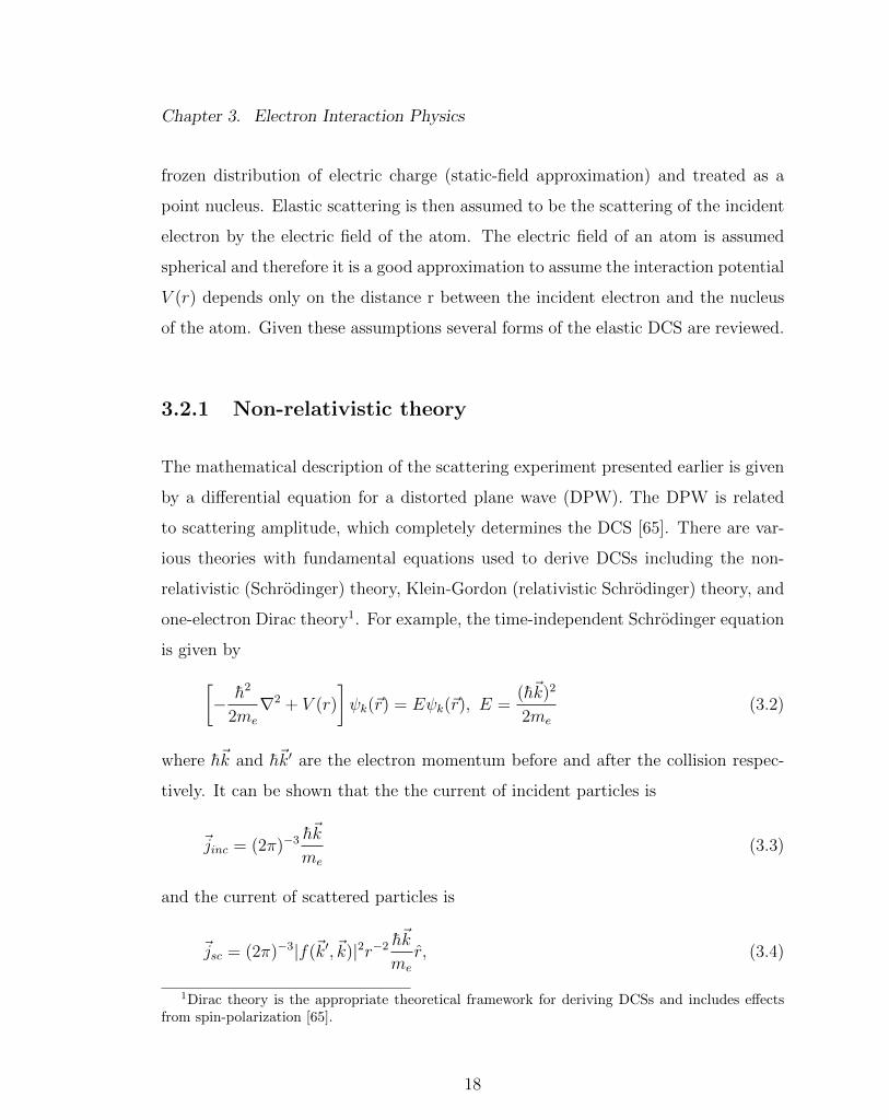
3.2.1 Non-relativistic theory
The mathematical description of the scattering experiment presented earlier is given
by a differential equation for a distorted plane wave (DPW). The DPW is related
to scattering amplitude, which completely determines the DCS [65]. There are var-
ious theories with fundamental equations used to derive DCSs including the non-
relativistic (Schrodinger) theory, Klein-Gordon (relativistic Schrodinger) theory, and
one-electron Dirac theory1. For example, the time-independent Schrodinger equation
is given by[− h2
2me
∇2 + V (r)
]ψk(~r) = Eψk(~r), E =
(h~k)2
2me
(3.2)
where h~k and h~k′ are the electron momentum before and after the collision respec-
tively. It can be shown that the the current of incident particles is
~jinc = (2π)−3 h~k
me
(3.3)
and the current of scattered particles is
~jsc = (2π)−3|f(~k′, ~k)|2r−2 h~k
me
r, (3.4)
1Dirac theory is the appropriate theoretical framework for deriving DCSs and includes effectsfrom spin-polarization [65].
18

Chapter 3. Electron Interaction Physics
where the scattered current is related to the count rate by Ncount = (~jsc · r)r2.
Therefore, for non-relativistic (Schrodinger) theory, Eq. (3.1) becomes
σel =Ncount
|~jinc|dΩ= |f(~k′, ~k)|2, (3.5)
where f(~k′, ~k) is the scattering amplitude and θ = arccos(~k′ ·~k) is the angle through
which the electron was scattered. Under these conditions, the scattering amplitude
is
f(~k′, ~k) = −4πme
h2
∫φ∗k′(~r)V (r)ψk(~r)d~r, (3.6)
where the interaction potential and the DPW appear again. Eq. (3.6) indicates that
the scattering amplitude, which completely determines the elastic DCS, is strongly
dependent on the scattering potential. Therefore, the most accurate representation
of the scattering potential possible is ideal. However, in the following sections one
will find that analytical expressions for the elastic DCS requires relatively simple
scattering potentials.
3.2.2 Screened Rutherford and classical Rutherford
It is impractical to obtain solutions to Eq. (3.2), so an alternative is to use the Born
Approximation. In the Born approximation, the Schrodinger equation is transformed
into an integral equation or
ψk(r) = φ(r) +
∫dr′G0(E, r, r′)V (r′)ψk(r), (3.7)
with the Green function
G0(E, r, r′) = − me
2πh2
exp(ik|r − r′|)|r − r′|
. (3.8)
The Born approximation starts with the zeroth-order approximation to Eq. (3.7) or
ψB0k (r) = φ(r). This is substituted into Eq. (3.7) to get the first order approximation
19

Chapter 3. Electron Interaction Physics
or
ψB1k (r) = φ(r) +
∫dr′G0(E, r, r′)V (r′)ψB0
k (r). (3.9)
This process is repeated to any order, but first and second order Born approximations
are the most common because beyond second order the approximation becomes un-
manageable. To obtain a familiar DCS, i.e. the screened Rutherford DCS, we begin
by applying the first-order Born approximation to the time-independent Schrodinger
equation. From this, the Schrodinger-Born scattering amplitude is obtained which
is given by
f (SB)(θ) = −2me
h2
∫ ∞0
sin(qr′)
qr′V (r′)r′2dr′. (3.10)
We then assume the Wentzel potential for a screening radius of R = a0Z−1/3 or
VW (r) =Z0Ze
2
rexp(−r/R). (3.11)
This results in the corresponding Born scattering amplitude or
f(SB)W (θ) = −2Ze2me
h2
1
(1/R)2 + q2, (3.12)
where
q = 2k
√1− cos θ
2(3.13)
for potential scattering. Therefore, the Wentzel or the “screened Rutherford” DCS
is
σWel (θ) = |f (SB)W (~k′, ~k)|2 =
(Ze2
2E
)21
[(2kR)−2 + (1− cos θ)]2(3.14)
where (2kR)−2 accounts for the screening of nucleus by the atomic electrons and k
is the electron wave number, Z atomic number of the target and e is the electron
charge. The classical Rutherford DCS is obtained by letting R→∞, which reduces
the Wentzel potential to a Coulomb potential, VC(r) = Ze2/r, where the effects of
nuclear screening are neglected. This gives,
σCel(θ) = |f (SB)W (~k′, ~k)|2 =
(Ze2
2E
)21
(1− cos θ)2(3.15)
20

Chapter 3. Electron Interaction Physics
3.2.3 Relativistic screened Rutherford
In practice, the classical Rutherford DCS is not used as it is singular about θ = 0.
The screened Rutherford DCS is not typically used either as it is non-relativistic.
However, Eq. (3.14) is easily generalizable to the relativistic formulation. At this
stage, it is convenient to define a new variable, the deflection cosine, or µ = cos θ.
The relativistic screened Rutherford (SR) DCS is given by
σSRel (E, µ) =(τ + 1)2
τ 2(τ + 2)2
C
[1 + 2η(E)− µ]2, (cm2sr−1), (3.16)
where the parameter C is a material constant given by
C = 2πr20Z
2N , (atoms cm−1), (3.17)
and the screening parameter [66] due to Moliere is
η(E) =0.25Z2/3
(0.885 · 137)2τ(τ + 2)
[1.13 + 3.76
(Z
137
)2(τ + 1)
τ(τ + 2)
], (3.18)
which is an improvement over the screening term that appeared in Eq. (3.14).
The peakedness of the SR DCS is a function of both energy and the target material
atomic number. Since the screening parameter drives the shape of the SR DCS, it
is insightful to understand the dependence of the screening parameter on energy
and atomic number which is given in Fig. 3.2. That is, as the screening parameter
approaches zero, the SR DCS becomes highly forward peaked or anisotropic and
nearly singular about unity. As the screening parameter grows larger, the SR DCS
becomes isotropic. As seen in Fig. 3.2, the screening parameter is dependent on
particle energy and the target material atomic number. Over a single decade in
energy, the screening parameter varies by roughly an order of magnitude. For the
same energy, over all materials, the screening parameter again varies a few orders
of magnitude. The magnitude of screening parameter indicates the strength of the
nuclear screening. Since the screening parameter is largest for high-Z materials and
21
Chapter 3. Electron Interaction Physics
10−2
10−1
100
101
102
10−10
10−8
10−6
10−4
10−2
100
E (MeV)
η(E
)
H
Be
Al
Cu
Fe
Au
U
Figure 3.2: Screening parameter for various materials
lower energies, nuclear screening has the greatest impact in this regime. For higher
energies and low-Z materials, the effect of nuclear screening is weak and the nucleus
begins to appear bare to the incident electron.
The following figures demonstrate the impact of the screening parameter on the
peakedness of the SR DCS. The SR DCS is most peaked for high-energy particles on
low-Z targets as seen in Fig. 3.3a and effectively isotropic for low-energy particles
on high-Z materials as seen in Fig. 3.3b. The screening parameter is a function
of energy and target Z, so this implies that the peakedness of elastic scattering is
generally driven by energy and target Z. This is made clear in the next section for
the partial-wave (PW) DCS, which does not depend on a screening parameter but
still demonstrates this same behavior.
22

Chapter 3. Electron Interaction Physics
0 20 40 60 80 100 120 140 160 18010
−30
10−25
10−20
10−15
10−10
θ (deg)
σn(θ
) (c
m2/s
r)
20−MeV, Al
1.051−MeV, Al
1.026−keV, Al
(a) Aluminum
0 20 40 60 80 100 120 140 160 180
10−30
10−25
10−20
10−15
10−10
θ (deg)
σn(θ
) (c
m2/s
r)
20−MeV, Au
1.051−Mev, Au
1.026−keV, Au
(b) Gold
Figure 3.3: Screened Rutherford (SR) DCS for elastic scattering of 1.026-keV, 1.051-MeV, and 20-MeV electrons by aluminum and gold nuclei.
3.2.4 Partial-wave DCS
In contrast to the time-independent Schrodinger equation, the Dirac equation is for
relativistic waves. It describes all spin-1/2 particles and is consistent with both the
principles of quantum mechanics and special relativity. For this reason, DCSs derived
from the Dirac equation are intrinsically better representations of elastic scattering.
Furthermore, the accuracy of the static-field approximation - used in previous sec-
tions to develop the screened Rutherford DCS - is limited by inelastic absorption and
charge-polarization effects [18]. Inelastic absorption causes a reduction of the elastic
DCS at intermediate and large angles that can be described by means of an approx-
imate absorptive potential. Furthermore, as a result of charge-polarization effects,
the charge distribution of the target is polarized by the electric field of the elec-
tron [18]. In turn, the electric field of the induced dipole acts back on the electron.
This can be described approximately by means of a local correlation-polarization
potential, which impacts the elastic DCS mostly at small angles. Thus, the effec-
tive interaction potential is described by an optical-model potential that includes the
electrostatic potential, the exchange potential, the correlation-polarization potential,
23

Chapter 3. Electron Interaction Physics
and the imaginary absorptive potential, is given by
V (r) = Vst(r) + Vex(r) + Vcp(r)− iWabs(r). (3.19)
The scattering of relativistic electrons by an interaction potential V (r) with a
finite range (V (r) = 0, r > rc) is completely described by the scattering amplitude
f(θ) and the spin-flip amplitude g(θ), which are solutions to the time-independent
Dirac equation for a given interaction potential V (r) [65]. That is,
σel = |f(θ)|2 + |g(θ)|2. (3.20)
It can be shown that after some tedious manipulations (see ICRU 77 appendices [65]
and references therein) that the scattering amplitude and the spin-flip amplitude
have the following form
f(θ) =1
2ik
∞∑`=0
(`+ 1)[exp(2iδk=`−1)− 1] + `[exp(2iδk=`)]P`(cos(θ) (3.21)
and
g(θ) =1
2ik
∞∑`=0
[exp(2iδk=`) + exp(2iδk=`−1)− 1]P 1` (cos(θ), (3.22)
where δk are the phase-shifts and determined from the asymptotic behavior of the
radial Dirac equations. That is,
PEk ∼ sin(kr − `π
e+ δk
)(3.23)
where PEk is a radial function and satisfies the radial Dirac equation [65]. The point
of being pedantic is to illustrate the need for a numerical calculation to determine the
phase-shifts, the scattering amplitude, and the spin-flip amplitude. That is, there
are no analytical representations of the phase-shifts, the scattering amplitude, and
the spin-flip amplitude without applying an approximation (e.g. the Born Approxi-
mation), so they must be calculated numerically.
24

Chapter 3. Electron Interaction Physics
Though Eqs. (3.21) and (3.22) do not have an analytical form, which introduces
additional considerations from the standpoint of working with DCS data, PW DCSs
are the most accurate representation of elastic scattering available outweighing the
difficulties associated with DCS data. The following PW DCSs and the DCS data
used for this study were generated using the ELSEPA computer code [18]. The PW
DCSs were generated using the following parameters:
• The Fermi nuclear charge distribution model
• The numerical Dirac-Fock electron distribution model
• The free atom model
• The Furness-McCarthy exchange potential
• The local-density approximation for correlation-polarization potential
• Measured dipole polarizability
• No absorption correction.
Examples of the PW DCS are presented in Fig. 3.4a and 3.4b. In Fig. 3.5, the
PW DCS and the SR DCS are compared. There are distinct differences between the
SR DCS and the PW DCS. The PW DCS are at least an order of magnitude more
peaked and the tail of the higher energy PW DCSs tend to fall-off more rapidly.
Furthermore, at low energies the PW DCS have distinct structure at large scattering
angles resulting from absorption effects. In addition to differences in the behavior
of the two DCSs, the moments also behave differently. Most importantly, the total
cross-section associated with the PW DCS is larger, while the mean deflection cosine
tends to be closer to unity.
25
Chapter 3. Electron Interaction Physics
0.0001 0.01 1
10−30
10−28
10−26
10−24
10−22
10−20
10−18
10−16
10−14
10−12
θ (degrees)
σel(E
,θ)
(cm
2/s
r)
10 50 100 150
1−keV
10−keV100−keV
1000−keV10000−keV20000−keV
(a) Aluminum
0.0001 0.01 1
10−28
10−26
10−24
10−22
10−20
10−18
10−16
10−14
10−12
10−10
θ (degrees)
σel(E
,θ)
(cm
2/s
r)
10 50 100 150
1−keV
10−keV100−keV
1000−keV10000−keV20000−keV
(b) Gold
Figure 3.4: Partial-wave differential cross-sections for the elastic scattering of 1-keV,10-keV, 100-keV, 1000-keV, and 10000-keV electrons by aluminum and gold atoms.
0.0001 0.01 1
10−26
10−24
10−22
10−20
10−18
10−16
10−14
10−12
θ (degrees)
Σel (
cm
2/s
r)
10 50 100 150
1−keV
10000−keV
100−keV
Solid Curve PWE
Dashed Curve screened Rutherford
Figure 3.5: Comparison of the relativistic screened Rutherford and partial-wavedifferential cross-sections for elastic scattering of 1-keV, 100-keV, and 10000-keVelectrons by gold atoms.
26
Chapter 3. Electron Interaction Physics
3.3 Inelastic Collisions with Atomic Electrons
Inelastic collisions with atomic electrons result in a transfer of energy from the inci-
dent electron to the atomic electron producing excitations or ionizations. Just as in
the case of elastic scattering, there is a variety of inelastic DCSs ranging in accuracy
and validity. The most basic form is the Rutherford inelastic DCS and typically
improvements upon Rutherford all contain a Rutherford-like term. For example, the
inelastic DCS used in this work, or the Moller DCS, introduced into the Rutherford
cross-section the effects of quantum-mechanical exchange, and of relativity, by treat-
ing the problem of the collision between two free electrons, using the relativistic Dirac
Theory of the electron [19]. Though Moller is an improvement over Rutherford, it is
really only valid for energy transfers that are large compared to the mean ionization
potential [67]. Therefore, some modifications to the Moller DCS are necessary for
agreement with experimental benchmarks. Of course, advanced inelastic DCSs are
utilized in codes like PENELOPE [27] that improve agreement with experiment, but
for the purposes of this work the modified Moller DCS is sufficient.
3.3.1 Moller
The energy loss DCS for binary collisions of electrons with free electrons at rest,
obtained from the Born approximation, is given by the Moller formula [27]. The
Moller inelastic DCS in which the incident electron with energy E transfers the
energy Q to the slower electron is given by
σin(E,Q) =
Kβ2
[1Q2 + 1
(E−Q)2 + 1(E+m0c2)
− m0c2(2E+m0c2)Q(E−Q)(E+m0c2)2
]: Q ∈ [Qmin, Qmax]
0 , otherwise,
(3.24)
27

Chapter 3. Electron Interaction Physics
where the lower bound, Qmin, is taken to be the mean ionization potential and the
upper bound, Qmax = E/2. In Figs. 3.6a and 3.6b we present the Moller DCS for
electrons of various energies scattered by aluminum and gold respectively. Like the
elastic scattering DCS, the inelastic DCS is peaked about small changes in state or
Qmin. As a function of incident particle energy, the inelastic DCS does not appear to
change significantly in shape. In fact, the impact of the incident electron energy is
subtle, as the inelastic DCS is inversely proportional to β2 which varies slowly above
500-keV and is roughly unity, but grows large as E → Qmin. Hence, the subtle peak
at Σin(E < 0.5MeV,Qmin). Moreover, the Moller DCS does not differ appreciably
from the Rutherford inelastic DCS except for relativistic energies and at Q ∼ Qmax.
The difference appears in the tail of the distribution making Moller slightly more
peaked. As a function of Z, the Moller DCS becomes slightly less peaked. This can
be seen by looking closely at the magnitude of the DCSs in Figs. 3.6a and 3.6b.
05
1015
20
02
46
810
10−28
10−26
10−24
10−22
10−20
10−18
10−16
E (MeV)Q (MeV)
σe
−(E
,Q)
(cm
2M
eV
−1)
(a) Aluminum
05
1015
20
02
46
810
10−28
10−26
10−24
10−22
10−20
10−18
E (MeV)Q (MeV)
σe
− (
E,Q
) (c
m2M
eV
−1)
(b) Gold
Figure 3.6: Moller inelastic DCS for scattering electrons by aluminum and gold.
In this work, we correct the Moller DCS such that the first moment of Moller is
28
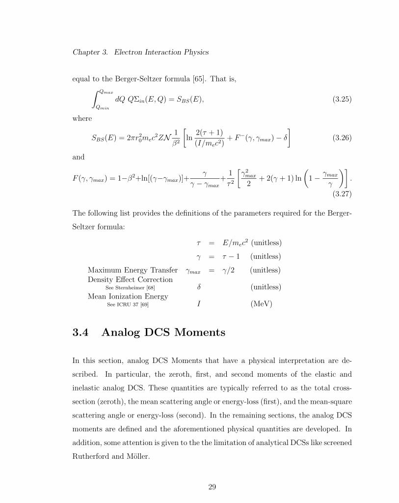
Chapter 3. Electron Interaction Physics
equal to the Berger-Seltzer formula [65]. That is,∫ Qmax
Qmin
dQ QΣin(E,Q) = SBS(E), (3.25)
where
SBS(E) = 2πr20mec
2ZN 1
β2
[ln
2(τ + 1)
(I/mec2)+ F−(γ, γmax)− δ
](3.26)
and
F (γ, γmax) = 1−β2+ln[(γ−γmax)]+γ
γ − γmax+
1
τ 2
[γ2max
2+ 2(γ + 1) ln
(1− γmax
γ
)].
(3.27)
The following list provides the definitions of the parameters required for the Berger-
Seltzer formula:
τ = E/mec2 (unitless)
γ = τ − 1 (unitless)
Maximum Energy Transfer γmax = γ/2 (unitless)Density Effect Correction
See Sternheimer [68] δ (unitless)Mean Ionization Energy
See ICRU 37 [69] I (MeV)
3.4 Analog DCS Moments
In this section, analog DCS Moments that have a physical interpretation are de-
scribed. In particular, the zeroth, first, and second moments of the elastic and
inelastic analog DCS. These quantities are typically referred to as the total cross-
section (zeroth), the mean scattering angle or energy-loss (first), and the mean-square
scattering angle or energy-loss (second). In the remaining sections, the analog DCS
moments are defined and the aforementioned physical quantities are developed. In
addition, some attention is given to the the limitation of analytical DCSs like screened
Rutherford and Moller.
29

Chapter 3. Electron Interaction Physics
3.4.1 Elastic DCS moments
Herein, we define Legendre moments of the elastic DCS as
Σel,` = 2π
∫ 1
−1
Pl(µ0)Σel(E, µ0)dµ0, (3.28)
and the momentum transfer moments as
G` = Σel,0 − Σel,`, (3.29)
where Σel,0 is the total macroscopic elastic cross-section with units of cm−1 and
defined as
Σel,0 = 2π
∫ 1
−1
Σel(E, µ0)dµ0. (3.30)
The macroscopic elastic total cross section, presented in Fig. 3.7a, gives the prob-
ability of an elastic interaction occurring per unit distance and is extremely large
for electrons. The microscopic total cross-section in barns is between 106-108. Con-
trast this to the total microscopic elastic cross section for neutrons that is typically
between 102 to 104 barns for a wide range of materials and energies.
In Fig. 3.7a, one can see the impact of the approximations required to obtain
the relativistic screened Rutherford DCS. Relativistic screened Rutherford is smaller
in magnitude for all energies. As a function of increasing energy, both relativistic
screened Rutherford and the partial-wave DCS monotonically decrease and eventu-
ally saturate. However, for decreasing energies, the partial-wave total cross-section is
monotonically increasing, whereas relativistic screened Rutherford begins to fall-off
for sufficiently low energies. This is a result of the validity of the Born approximation,
which is valid for(Z
137β
)2
<< 1. (3.31)
One can see the impact of Z on the validity of the Born approximation in Fig. 3.7a
where the relativistic screened Rutherford total cross-section begins to diverge from
30
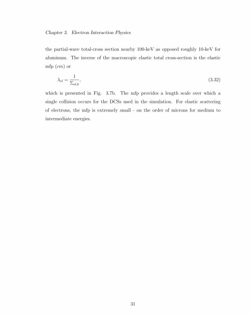
Chapter 3. Electron Interaction Physics
the partial-wave total-cross section nearby 100-keV as opposed roughly 10-keV for
aluminum. The inverse of the macroscopic elastic total cross-section is the elastic
mfp (cm) or
λel =1
Σel,0
, (3.32)
which is presented in Fig. 3.7b. The mfp provides a length scale over which a
single collision occurs for the DCSs used in the simulation. For elastic scattering
of electrons, the mfp is extremely small - on the order of microns for medium to
intermediate energies.
31

Chapter 3. Electron Interaction Physics
10−3
10−2
10−1
100
101
105
106
107
108
109
Energy (MeV)
σel,
0 (
barn
s)
Screened Rutherford, Al
Screened Rutherford, Au
Partial−wave, Al
Partial−wave, Au
(a) Total Cross-Section
10−3
10−2
10−1
100
101
10−8
10−7
10−6
10−5
10−4
10−3
10−2
Energy (MeV)
λel (
cm
)
Screened Rutherford, Al
Screened Rutherford, Au
Partial−wave, Al
Partial−wave, Au
(b) Mean Free Path
Figure 3.7: Screened Rutherford and partial-wave total cross-sections and mean freepaths for elastic collisions with aluminum and gold nuclei.
The mean scattering angle or
µ0 =Σel,1
Σel,0
, (3.33)
is related to the transport cross-section, or G1, by
G1 = Σel,0 − Σel,1 = Σel,0(1− µ0) (3.34)
The transport cross-section is the inverse transport mfp (cm) or
λtr =1
Σel,1
. (3.35)
The transport mfp, presented in Fig. 3.8, provides a length scale over which an
initially singular beam experiences significant spreading in space, angle, and energy.
The ratio of the transport cross section to the total cross section is known and the
scattering power of the medium. Under conditions of highly peaked scattering one
can invoke the small angle approximation to further understand the significance of
the transport cross-section. That is,
G1 ≈ 2π
∫ π
0
θ20
2Σel(E, θ0) sin θ0dθ0 = 〈θ2
0〉, (3.36)
where 〈θ20〉 is the mean-square scattering angle and is related to the spreading of a
beam. That is, the beam broadens with increasing 〈θ20〉.
32
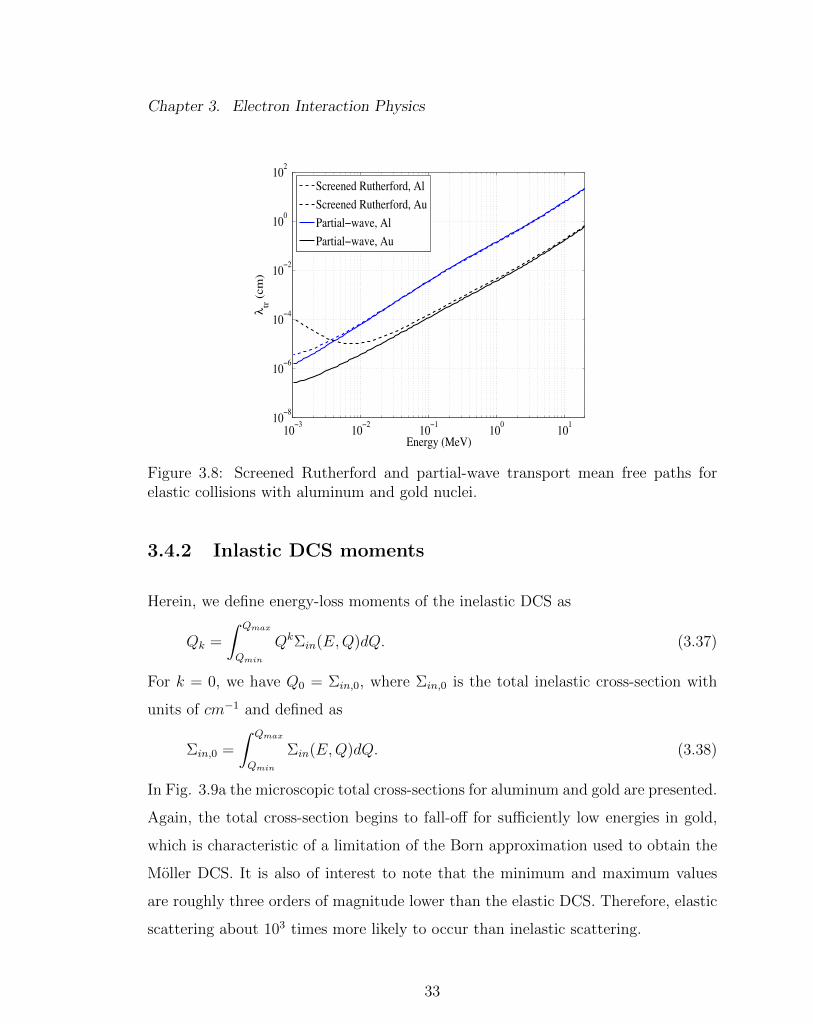
Chapter 3. Electron Interaction Physics
10−3
10−2
10−1
100
101
10−8
10−6
10−4
10−2
100
102
Energy (MeV)
λtr (
cm
)
Screened Rutherford, Al
Screened Rutherford, Au
Partial−wave, Al
Partial−wave, Au
Figure 3.8: Screened Rutherford and partial-wave transport mean free paths forelastic collisions with aluminum and gold nuclei.
3.4.2 Inlastic DCS moments
Herein, we define energy-loss moments of the inelastic DCS as
Qk =
∫ Qmax
Qmin
QkΣin(E,Q)dQ. (3.37)
For k = 0, we have Q0 = Σin,0, where Σin,0 is the total inelastic cross-section with
units of cm−1 and defined as
Σin,0 =
∫ Qmax
Qmin
Σin(E,Q)dQ. (3.38)
In Fig. 3.9a the microscopic total cross-sections for aluminum and gold are presented.
Again, the total cross-section begins to fall-off for sufficiently low energies in gold,
which is characteristic of a limitation of the Born approximation used to obtain the
Moller DCS. It is also of interest to note that the minimum and maximum values
are roughly three orders of magnitude lower than the elastic DCS. Therefore, elastic
scattering about 103 times more likely to occur than inelastic scattering.
33
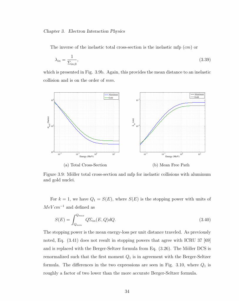
Chapter 3. Electron Interaction Physics
The inverse of the inelastic total cross-section is the inelastic mfp (cm) or
λin =1
Σin,0
, (3.39)
which is presented in Fig. 3.9b. Again, this provides the mean distance to an inelastic
collision and is on the order of mm.
10−2
10−1
100
101
104
105
106
Energy (MeV)
σin
,0 (
barn
s)
Aluminum
Gold
(a) Total Cross-Section
10−2
10−1
100
101
10−4
10−3
Energy (MeV)
λin
(cm
)
Aluminum
Gold
(b) Mean Free Path
Figure 3.9: Moller total cross-section and mfp for inelastic collisions with aluminumand gold nuclei.
For k = 1, we have Q1 = S(E), where S(E) is the stopping power with units of
MeV cm−1 and defined as
S(E) =
∫ Qmax
Qmin
QΣin(E,Q)dQ. (3.40)
The stopping power is the mean energy-loss per unit distance traveled. As previously
noted, Eq. (3.41) does not result in stopping powers that agree with ICRU 37 [69]
and is replaced with the Berger-Seltzer formula from Eq. (3.26). The Moller DCS is
renormalized such that the first moment Q1 is in agreement with the Berger-Seltzer
formula. The differences in the two expressions are seen in Fig. 3.10, where Q1 is
roughly a factor of two lower than the more accurate Berger-Seltzer formula.
34

Chapter 3. Electron Interaction Physics
10−2
10−1
100
101
100
101
102
Energy (MeV)
Sto
pp
ing
Po
wer
(M
eV/c
m)
Q1, Au
Berger−Seltzer, Au
Q1, Al
Berger−Seltzer, Al
Figure 3.10: Stopping power from Eq. (3.41) and the Berger-Seltzer formula.
For k = 2, we have Q2 = T (E), where T (E) is the straggling coefficient with
units of MeV 2cm−1 and defined as
T (E) =
∫ Qmax
Qmin
Q2Σin(E,Q)dQ. (3.41)
Energy straggling is the result of occasional inelastic collisions resulting in large
energy-losses. In an energy-loss simulation for a thin slab where stopping power is
applied in a CSD fashion, the resulting energy spectra will be singular and equal
to the mean energy-loss. By including straggling, there will be a spread in energy
about the mean energy-loss. The amount of spreading will depend on the strength
of the energy straggling. Straggling impacts quantities like dose from electrons by
smoothing out the Bragg peak.
35
Chapter 4
The Analog Problem
In this chapter, the challenges associated with the analog electron transport are ex-
pressed. That is, the challenges associated with solving the transport equation where
the interaction physics are given by the single-scatter or analog DCSs described in
Chapter 3. To understand the challenges it is necessary to describe the transport
equation in some detail. To do so, a description of the independent variables as-
sociated with the transport equation, along with a discussion of the angular flux
(that is, the solution) and quantities of interest that are derived from the angular
flux are provided. Rather than deriving the transport equation, which can be found
in numerous particle transport texts [11, 70], the transport equation of interest is
written down and qualitative descriptions of the various terms that appear are pro-
vided. Furthermore, a summary of the Monte Carlo algorithm for electron transport
is presented within the context of the Geant4 toolkit [3]. The chapter is concluded
with example calculations corresponding to the aforementioned derived quantities
using analog Monte Carlo, along with the computer time required to complete such
calculations. The computational cost associated with analog Monte Carlo transport
of electrons with moderate to high energies is the single-most important reason for
developing efficient approximate methods.
36

Chapter 4. The Analog Problem
4.1 Independent Variables
It is of interest to obtain solutions to the 3-D transport equation. The solution,
or the angular flux, is the distribution of particles in a six-dimensional phase-space
including position ~r, energy E, and direction ~Ω, at some time t, where the position
with respect to the origin in Cartesian coordinates is given by
~r = xi+ yj + zk. (4.1)
A differential hexahedral volume, dV , is obtained by sweeping out an incremental
amount in all directions about ~r and given by dV = dxdydz.
The direction, measured with respect to the polar angle, θ, and azimuthal angle,
ϕ, is given by
~Ω = Ωxi+ Ωy j + Ωzk, (4.2)
where
Ωx = (1− cos θ)1/2 cosϕ
Ωz = (1− cos θ)1/2 sinϕ
Ωy = cos θ.
(4.3)
An incremental differential surface on the unit sphere, dΩ, is swept out about ~Ω and
given by dΩ = dµdϕ, where µ = cos θ and dµ is an incremental displacement with
respect to the polar angle, while dϕ is an incremental displacement with respect to
the azimuthal angle.
37
Chapter 4. The Analog Problem
4.2 The Angular Particle Density and Derived Quan-
tities
The angular particle density describes a population of particles in the phase space
of interest. The angular flux, or the solution to the transport equation, is related to
the angular particle density. Numerous quantities of interest are derived from the
angular flux. The angular particle density and various derived quantities are the
subject of the following sections.
4.2.1 The angular particle density
The angular particle density is denoted asN(~r, E, ~Ω, t), whereN(~r, E, ~Ω, t)dV dEdΩdt
gives the number of particles in dV dEdΩ about (~r, E, ~Ω) at time t with units of
(cm−3MeV −1). The quantity of interest, the angular flux, is related to the angular
particle density by
ψ(~r, E, ~Ω, t) = vN(~r, E, ~Ω, t), (4.4)
where v is the particle velocity. Therefore, the volume based interpretation of the
angular flux, or ψ(~r, E, ~Ω, t)dV dEdΩ, is the rate at which path length is generated
by particles in dV dEdΩ about (~r, E, ~Ω) at time t with units of (cm−2MeV −1s−1).
Many other derived quantities follow from the angular flux or the scalar flux
which is given by
φ(~r, E, t) =
∫4π
dΩψ(~r, E, ~Ω, t), (4.5)
and is the zeroth angular moment of the angular flux. For example, quantities of
interest presented in the results section include angular distributions, energy spectra,
longitudinal and lateral distributions, dose or energy deposition, charge deposition,
38

Chapter 4. The Analog Problem
and transmission and reflection fractions. Each of these quantities are defined in the
following sections.
4.2.2 Derived quantities
It is uncommon to require the angular flux directly. Typically, quantities derived
from the angular flux are of direct use. This includes quantities like angular distri-
butions, energy spectra, longitudinal and lateral distributions, dose, charge deposi-
tion, and reflection and transmission fractions. These quantities are now described
in greater detail and and in many cases, the result is a function p indicating that
these distributions can be interpreted as probability distribution functions.
Angular distributions
Angular distributions at some position ~r are typically a function of the polar angle θ
or µ = cos θ, which requires integration of the angular flux over all azimuthal angles
and energies or
p(~r, µ) =
∫ 2π
0
dφ
∫ ∞0
dEψ(~r, E, φ, µ). (4.6)
Though p(~r, µ) can be obtained at any position, it is common in electron transport
to obtain reflected and transmitted angular distributions in thin slabs. For a 1-D
slab of thickness L with the left face at the origin, the reflected and transmitted
distributions are given by
p(0, µ) =
∫ 2π
0
dφ
∫ ∞0
dEψ(0, E, φ, µ), (4.7)
and
p(L, µ) =
∫ 2π
0
dφ
∫ ∞0
dEψ(L,E, φ, µ) (4.8)
39

Chapter 4. The Analog Problem
respectively. Note that particles traveling in directions with µ > 0 do not contribute
to the reflected distribution, while particles traveling in directions with µ < 0 do not
contribute to the transmitted distribution.
Energy spectra
Energy spectra at some position ~r are a function of particle energy and an angular in-
dependent quantity that requires integration of the angular flux over all contributing
angles. This quantity is effectively an energy dependent current, J(~r, E), or
J(~r, E) =
∫~Ω·n>0
dΩ
∫∂R
dS (~Ω · n)ψ(~r, E, φ, µ)
−∫~Ω·n<0
dΩ
∫∂R
dS |~Ω · n|ψ(~r, E, φ, µ).
(4.9)
Once again, it is common in electron transport to obtain reflected and transmitted
energy spectra in thin slabs. In this case, the definition of an energy dependent
partial current is necessary where particles flowing in positive directions ~Ω · n > 0
across a surface element ∂S contribute to the positive partial current
J+(~r, E) =
∫~Ω·n>0
dΩ
∫∂R
dS ~Ω · nψ(~r, E, φ, µ), (4.10)
and particles flowing in negative ~Ω · n < 0 directions across a surface element ∂S
contribute to the negative partial current
J−(~r, E) =
∫~Ω·n<0
dΩ
∫∂R
dS |~Ω · n|ψ(~r, E, φ, µ), (4.11)
where n is a unit vector normal to the surface of flow. Therefore, in the 1-D slab
described in section 4.2.2, the reflected energy spectrum is
p(0, E) = J−(0, E), (4.12)
and the transmitted energy spectrum is
p(L,E) = J+(L,E). (4.13)
40

Chapter 4. The Analog Problem
In many cases, one is interested in energy-loss spectra as well which are given by
p(0, E0 − E) = J−(0, E0 − E), (4.14)
and
p(L,E0 − E) = J+(L,E0 − E), (4.15)
where E0 is the initial energy of the particle.
Longitudinal and lateral distributions
Longitudinal and lateral distributions are closely related to Lewis theory. In fact,
these distributions are obtained by solving an infinite medium transport equation
for mono-energetic particles. The longitudinal distribution is
p(z, s) =
∫ ∞−∞
dx
∫ ∞−∞
dy
∫4π
dΩψ(x, y, z, s, ~Ω), (4.16)
and gives the probability that a particle will be displaced a distance ±z along the
axis of the initial direction of the particle given some pathlength s. The lateral
distribution is
p(b, s) =
∫ ∞−∞
dz
∫4π
dΩψ(x, y, z, s, ~Ω), (4.17)
where b =√x2 + y2 and gives the probability that a particle will be displaced
laterally through a distance b orthogonal to the axis of the initial direction of the
particle pathlength s. That is, the radial spread given some pathlength s.
Dose deposition
The dose gives the spatial distribution of the energy deposited per unit volume. It is
obtained by integrating the product of the average energy lost per distance traveled,
41
Chapter 4. The Analog Problem
S(E), or the stopping power and the flux over all energies and angles or
D(~r) =
∫4π
dΩ
∫ ∞0
dE S(E)ψ(~r, E, ~Ω) =
∫ ∞0
dE S(E)φ(~r, E), (MeV/cm3). (4.18)
This quantity is of particular interest to nearly all applications of electron transport.
Moreover, the dose is typically easier to resolve because it is only differential in space
in contrast to some of the previous quantities that are also differential in angle or
energy.
Charge deposition
Charge deposition is the spatial distribution of charge (positive or negative) produced
by a particle slowing down through energies less than Emin. Similar to dose, charge
deposition is related to the scalar flux or
C(~r) =
∫ ∞Emin
dE ′∫ Emin
0
dE ′′ Σin(E ′ → E ′′)φ(~r, E ′), (cm−3), (4.19)
where Emin is the energy below which particles are assumed deposited. Eq. (4.8)
can be interpreted as a slowing down density. The inner integral gives the rate at
which electrons with energies E ′ slow down past Emin. The outer integral then gives
the total slowing down density for all electrons with energies E ′ > Emin.
Reflection and transmission fractions
Reflection and transmission fractions are typically thin-slab results and are a mea-
sure of the number of source particles that are not absorbed in the medium and
either forward-scatter (transmission) or backscatter (reflection). For a 1-D slab (as
described in section 4.2.2), the reflection fraction is the negative partial current eval-
uated at x = 0 or
J−(0) =
∫ ∞0
dE
∫~Ω·n<0
dΩ
∫∂R
dS |~Ω · n|ψ(0, E, φ, µ). (4.20)
42

Chapter 4. The Analog Problem
and the transmission fraction is the positive partial current evaluated at x = L or
J+(L) =
∫ ∞0
dE
∫~Ω·n>0
dΩ
∫∂R
dS ~Ω · nψ(L,E, φ, µ) (4.21)
4.3 The Electron Transport Equation
Given the definitions from section 4.2, the usual practice is to derive the transport
equation by writing down an equation for the time rate of change in some incremental
population of particles which is related to the rate of loss and the rate of gain. That
is,
∂
∂tN(~r, E, ~Ω, t) = gains− losses. (4.22)
Next, the angular particle density is related to the angular density, ψ(~r, E, ~Ω, t) =
vN(~r, E, ~Ω, t), and the contributions to gains and losses are obtained from first prin-
ciples. Here, the transport equation for electrons is simply written down and each
term is discussed as it relates to gains and losses. If necessary, the reader should
refer to more complete derivations from the text [11, 70].
To begin, it is of interest to study the time-independent transport equation for
electrons. In this equation, it is assumed that the solution is not changing as a
function of time; therefore, particle losses are exactly balanced by particle gains and
Eq. (4.22) becomes a balance equation or
Ω · ∇ψ(~r, E, ~Ω) + [Σel,0(~r, E) + Σin,0(~r, E)]ψ(~r, E, ~Ω)
=
∫ ∞0
dE ′∫
4π
dΩ′[Σel(~r, E
′ → E, ~Ω′ · ~Ω) + Σin(~r, E ′ → E, ~Ω′ · ~Ω)]ψ(~r, E ′, ~Ω′)
(4.23)
where the left hand side corresponds to losses from leakage and out-scatter and the
right hand side corresponds to gains from in-scatter and secondary production. That
43

Chapter 4. The Analog Problem
is, Ω · ∇ψ(~r, E, ~Ω)dV dEdΩ is the net leakage of particles with energies in dE about
E and directions in dΩ about ~Ω from dV . The out-scatter is a loss due to particles in
dV dEdΩ about (~r, E, ~Ω) suffering an elastic or inelastic collision resulting in removal
of the particles from the energy or angular phase-space. The elastic and inelastic
in-scatter or∫∞
0dE ′
∫4πdΩ′[Σel(~r, E
′ → E, ~Ω′ ·~Ω)+Σin(~r, E ′ → E, ~Ω′ ·~Ω)]ψ(~r, E ′, ~Ω′)
is a gain from particles in dV dE ′dΩ′ about (~r, E ′, ~Ω′) scattering into dV dEdΩ about
(~r, E, ~Ω). Finally, Qδ(~r, E, ~Ω) is a gain due to production of secondary electrons in
dV dEdΩ about (~r, E, ~Ω).
It is customary to rewrite the transport equation in terms of the Boltzmann
collision operator or
Ω · ∇ψ(~r, E, ~Ω) = HBψ(~r, E, ~Ω) +Qδ(~r, E, ~Ω), (4.24)
where the Boltzmann collision operator is defined as
HBψ(~r, E, ~Ω) =
∫ ∞0
dE ′∫
4π
dΩ′[Σel(~r, E
′ → E, ~Ω′ · ~Ω)
+ Σin(~r, E ′ → E, ~Ω′ · ~Ω)]ψ(~r, E ′, ~Ω′)− Σt(~r, E)ψ(~r, E, ~Ω),
(4.25)
and Σt(~r, E) = Σel,0 + Σin,0. Eq. (4.24) is subject to the following general boundary
condition
ψ(~r, E, φ, µ) = ψb(~r, E, φ, µ), ~r ∈ ∂V, ~Ω(φ, µ) · ~n < 0, 0 < E <∞, (4.26)
For electrons, elastic and inelastic scattering are treated separately as indicated
in Eq. (4.25). Furthermore, it is assumed that elastic scattering occurs without
energy loss and angular deflection from inelastic scattering is given by kinematics,
so the collision operator can be expressed as
HBψ(~r, E, ~Ω) = HBelψ(~r, E, ~Ω) +HB
inψ(~r, E, ~Ω), (4.27)
44

Chapter 4. The Analog Problem
where
HBelψ(~r, E, ~Ω) =
∫4π
dΩ′Σel(~r, E, ~Ω′ · ~Ω)ψ(~r, E, ~Ω′)−Σel,0(~r, E)ψ(~r, E, ~Ω) (4.28)
and
HBinψ(~r, E, ~Ω) =
∫4π
dΩ′∫ ∞
0
dE ′Σin(~r, E ′ → E)δ[~Ω′ − f(E ′, Q)]ψ(~r, E ′, ~Ω′)
− Σin,0(~r, E)ψ(~r, E, ~Ω),
(4.29)
where the angle of the primary is
f(E,Q) =
√E −QE
E + 2mec2
E −Q+ 2mec2(4.30)
and the angle of the secondary is
g(E,Q) =
√Q
E
E + 2mec2
Q+ 2mec2. (4.31)
In the event that secondary production is neglected (Qδ = 0) and deflection of
the primary from inelastic scattering is also considered negligible, Eq. (4.29) reduces
to
HBelψ(~r, E, ~Ω) =
∫ ∞0
dE ′Σin(~r, E ′ → E)ψ(~r, E ′, ~Ω)−Σin,0(~r, E)ψ(~r, E, ~Ω). (4.32)
As previously mentioned, direct numerical solution of Eq. (4.24) is not realistic
for most applications of interest because of the large total cross sections, Σel,0 and
Σin,0, and DCSs, Σel and Σin, that are highly peaked about small deflections and
energy losses. Because the computational effort is related to the number of collisions
simulated per particle history and the outcome of the collision, simulation of Coulomb
collisions are far more computationally intensive than the interactions characterizing
neutral particles. Examples of analog electron transport calculations or solutions
to Eq. (4.23), along with the associated computational cost, is the subject of the
following section.
45

Chapter 4. The Analog Problem
4.4 Analog Monte Carlo Calculations
When applying the Monte Carlo method to the transport equation, it is possible to
obtain solutions by simulating the physical processes of particles without necessarily
writing down or referring to the transport equation. Furthermore, a Monte Carlo so-
lution does not include the fine detail that is characteristic of deterministic methods
(that is, the angular flux) but instead provides information about certain specified
quantities of interest (that is, derived quantities) [12]. Therefore, the Monte Carlo
method might be described as an intuitive or physical approach to solving the trans-
port equation through direct simulation of particle behavior, where the individual
particle interactions can be considered a Markov process which are independent of
their history.
Of course, one of the drawbacks of analog Monte Carlo is that the detailed physics
may be computationally prohibitive as in the case of electrons. In this section, we
demonstrate the computational cost associated with several analog Monte Carlo
solutions to the transport equation. Before presenting any results, the analog Monte
Carlo algorithm is summarized.
4.4.1 Analog Monte Carlo algorithm
What is generally required for an analog Monte Carlo calculation is a description of
the geometrical boundaries, a description of the material properties in each region,
and the differential and total cross-section for each material. In the algorithm de-
scribed below, it is assumed that particles travel straight lines between collisions,
particles suffer a collision per unit distance with probability Σt, the time during a
collision can be neglected, and the particle transport being simulated is linear [12].
In general, a particle is tracked from “birth” until its “death,” which starts by
46

Chapter 4. The Analog Problem
sampling a particle from the source description. The source can be a boundary
source, or boundary condition, and/or an internal source. Both boundary and inter-
nal sources can be functions of space, angle, and energy. Given a source particle, the
distance to collision is sampled according to exponentially distributed collision sites.
The particle is moved the distance to the next collision site in its current direction.
Assuming the particle did not leave the system, the collision type and the collision
outcome are sampled. This process is repeated until the particle is absorbed by the
medium or the particle leaves the system.
As with all probabilistic quantities - the source function, the differential cross-
section, the distance to collision, and so forth - they are determined by sampling
(direct, rejection) a probability density function (PDF), which requires deriving a
cumulative probability function (CDF). Details on direct and rejection sampling
techniques are given in reference [12] and references therein.
The following is an outline of the analog Monte Carlo algorithm specifically for
transporting electrons. The important steps are listed and some detail is given for
the quantity sampled at each step along with other applicable considerations.
Analog Monte Carlo algorithm
1. Sample source particle
– For monoenergetic pencil beams this simply requires initializing the
particles position r0, energy E0, and direction ~Ω0. For distributed
sources one must obtain a CDF and apply inverse mapping. For
example, for an isotropic point source the polar angle is determined by
µ← 2ξ1−1 and the azimuthal angle is determined by ϕ← 2πξ2 where
ξ1 and ξ2 are two different random numbers uniformly distributed
between zero and one.
2. Sample distance to collision
47

Chapter 4. The Analog Problem
– Distance to collision is generally given by s← − ln(ξ)/Σt, where Σt is
the probability per unit distance that an elastic or inelastic collision
will occur. Given the distance s and the current direction of the
particle Ωi, this must be compared with the distance to the next
boundary d.
∗ If s < d, the particle is moved to the collision site and algorithm
continues with step 3.
∗ If s ≥ d and the material on each side of the boundary is the same,
the residual s and d are compared and the particle is moved to
the collision site if the residual s < d and algorithm continues
with step 3.
∗ If s ≥ d and the material on each side of the boundary is different,
the particle is stopped at the boundary without colliding and
restart at step 2.
∗ If s ≥ d and the particle crosses a system boundary, the particle is
killed, quantities of interest are tallied, and the algorithm restarts
at step 1.
3. Sample collision type
– The collision type is sampled from the point probability associated
with each collision type. That is, the probability of the ith collision
type is pi = σi,0/σt, where∑
i pi = 1. As it relates to the analog
problems studied herein, the two point probabilities for elastic and
inelastic collisions are pel = σel,0/σt and pin = σin,0/σt. To determine
the collision type a random number is sampled and the following logic
is applied:
∗ If ξ ≤ pel, then an elastic collision occurred.
∗ Otherwise, an inelastic collision occurred.
48

Chapter 4. The Analog Problem
4. Sample collision outcome
– Given the collision type, the appropriate DCS is sampled according
to the necessary method (direct or rejection). For example, when
sampling screened Rutherford the direct method used is
µ0 ← 1 − 2ηξ/(1.0 − ξ + η). When sampling from the partial-wave
DCSs, methods for inverting discrete DCSs are used. Lastly, when
sampling Moller a rejection method must be used because the Moller
DCS cannot be inverted.
5. Update particle state
– Given the collision outcome, the particles energy or direction is up-
dated. In the event of an inelastic collision, some additional steps are
required. That is,
∗ If the sampled energy-loss is greater than the secondary produc-
tion threshold, a secondary must be generated.
∗ Otherwise, the energy-loss is assumed to be deposited locally and
tallied if necessary.
6. Restart at step 1.
4.4.2 Tallies
In Monte Carlo calculations, quantities of interest are obtained through tallies. That
is, counting events that contribute to some quantity being tracked. Each tally is
related to the derived quantities from section 4.2, but it is typically easier to use an
intuitive approach in obtaining expressions for tallies.
49

Chapter 4. The Analog Problem
Angular distributions
The particle’s polar angle is tallied when crossing a specified surface, when transmit-
ted, reflected, or after reaching a maximum specified pathlength. Angular Distribu-
tion tallies are determined by summing up all contributions by each particle to some
ith angular bin. If the polar angle of the jth particle is within the limits of the ith
bin, that bin is incremented by one. The expression for the angular distribution is
p(θi) =1
N∆θi
∑j
f(θj), (4.33)
where N is the number of source particles, ∆θi = θi+1/2 − θi−1/2, θi−1/2 and θi+1/2
are the lower and upper limit of the ith bin, and
f(θj) =
1 : θi−1/2 ≤ θj < θi+1/2
0 : otherwise.(4.34)
Energy-loss spectra
The particle’s energy-loss (Q=E0 − E) is tallied when crossing a specified surface,
when transmitted, reflected, or after reaching a maximum specified pathlength.
Energy-loss spectra tallies are determined by summing up all contributions by each
particle to some ith energy-loss bin. If the energy-loss of the jth particle is within
the limits of the ith bin, that bin is incremented by one. The expression for the
energy-loss spectra is
p(Ei) =1
N∆Qi
∑j
f(Qj), (4.35)
where N is the number of source particles, ∆Qi = Qi+1/2−Qi−1/2, Qi−1/2 and Qi+1/2
are the lower and upper limit of the ith bin, and
f(Qj) =
1 : Qi−1/2 ≤ Qj < Qi+1/2
0 : otherwise.(4.36)
50
Chapter 4. The Analog Problem
Longitudinal and lateral distributions
The particle’s longitudinal displacement (z/s) and lateral displacement
(b/s, b =√x2 + y2) is tallied when a particle reaches a maximum specified path-
length s. Longitudinal and lateral distribution tallies are determined by summing
up all contributions by each particle to some ith longitudinal or lateral displacement
bin. The expression for the longitudinal distribution is
p(zis
)=
1
N∆( zis
)
∑j
f(zjs
), (4.37)
where N is the number of source particles, ∆zi/s =zi+1/2
s− zi−1/2
s, and
f(zjs
)=
1 :zi−1/2
s≤ zj
s<
zi+1/2
s
0 : otherwise.(4.38)
The expression for the lateral distribution is
p
(bis
)=
1
N∆( bis
)
∑j
f
(bjs
), (4.39)
where N is the number of source particles, ∆bi/s =bi+1/2
s− bi−1/2
s, and
f
(bjs
)=
1 :bi−1/2
s≤ bj
s<
bi+1/2
s
0 : otherwise.(4.40)
Dose deposition
Dose tallies are determined by summing over all energy deposited in the ith spatial
cell, by the jth particle or
D(xi, yi, zi) =1
ρiVi
∑j
∆Ei,jN
, (4.41)
where ρi is the density of the material in the ith cell, Vi is the volume of the ith cell,
and ∆Ei,j is the energy deposited between xi and xi+1, yi and yi+1, and zi and zi+1
by the jth particle.
51

Chapter 4. The Analog Problem
Charge deposition
Charge deposition is tallied for the ith spatial bin when a particle slows down past
some minimum energy (negative charge) and when a secondary is created (positive
charge). The expression for charge deposition is
C(xi, yi, zi) =R0
rcNVi
∑j
f(cj), (4.42)
where N is the number of source particles, Vi is the volume of the ith cell, R0 is the
CSDA range of the particle, rc is the reflection factor given in the following section,
cj is −1 for charge deposition and 1 for secondary production, and
f(cj) =
cj : ~rj ∈ Vi0 : otherwise.
(4.43)
In other words, cj is tallied in the ith cell corresponding to where a charge was
deposited (cj = −1) or where a secondary was produced (cj = 1). The factor rc
is used to normalize the charge deposition such that the total charge deposition
(integration over all spatial dimensions) is unity.
Reflection and transmission fractions
Reflection and transmission fractions are typically calculated in thin slabs or semi
infinite slabs when a particle exits through the left face (reflection) or through the
right face (transmission). If a particle leaves the left face, the reflection tally is
incremented by one, so after N source particles the reflection fraction is
rc =1
N
∑j
fr(xj) (4.44)
where
fr(xj) =
1 : xj < 0
0 : otherwise.(4.45)
52
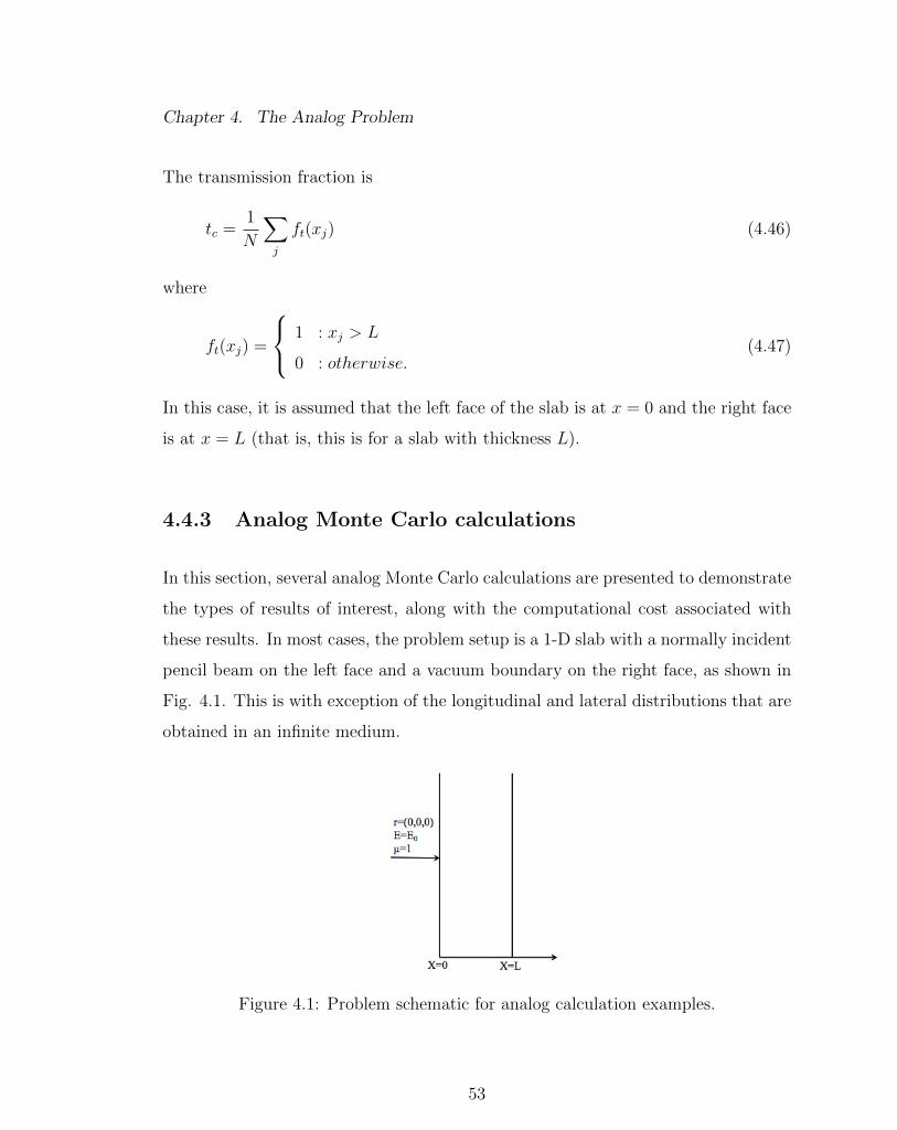
Chapter 4. The Analog Problem
The transmission fraction is
tc =1
N
∑j
ft(xj) (4.46)
where
ft(xj) =
1 : xj > L
0 : otherwise.(4.47)
In this case, it is assumed that the left face of the slab is at x = 0 and the right face
is at x = L (that is, this is for a slab with thickness L).
4.4.3 Analog Monte Carlo calculations
In this section, several analog Monte Carlo calculations are presented to demonstrate
the types of results of interest, along with the computational cost associated with
these results. In most cases, the problem setup is a 1-D slab with a normally incident
pencil beam on the left face and a vacuum boundary on the right face, as shown in
Fig. 4.1. This is with exception of the longitudinal and lateral distributions that are
obtained in an infinite medium.
Figure 4.1: Problem schematic for analog calculation examples.
53

Chapter 4. The Analog Problem
Table 4.1: Timing results for analog simulation of 106 1-MeV electrons normallyincident on aluminum and gold slabs with varying thicknesses. The slab thicknessespresented in cm corresponds to aluminum slabs, while the gold slabs are roughlyone-tenth the thickness of the aluminum slab. Note that the computer time scalesroughly linearly for aluminum, while scaling non-linearly for gold.
Timing results for analog simulation
SlabThickness
(mfp)
SlabThickness
(cm)
CPU TimeAl/Au(min)
100 0.0019 6/7300 0.0057 20/211000 0.019 72/1003000 0.057 273/384
In Table 4.1, the computer times required for analog simulation of 106, 1-MeV
electrons in aluminum and gold for varying slab thicknesses are presented. In general,
the slab thickness in Table 4.1 are very small (∼ mm − µm), so this problem is
not representative of the full spectrum of electron transport calculations. Even so,
for this small sampling of calculations the computer times for the simulations with
slab thicknesses ∼ mm are still on the order of one to six hours. This amount of
computer time is impractical for routine calculations; especially, considering that
these times are associated with just the transport of primary particles. That is,
no secondaries were produced in these example calculations. Secondary production
would only increase the amount of computer time required. The computer times
associated with the aluminum slabs scale linearly. However, in gold, as the slab
becomes thicker, inelastic collisions become more probable increasing the computer
time. This is because as particles lose energy the mfp of the particle decreases and
the particle suffers further collisions. Not to mention, inelastic collisions require a
rejection technique that is more costly than direct sampling. In the following sections,
several results associated with the computer times are provided to give a sense of
typical results and how they behave.
54
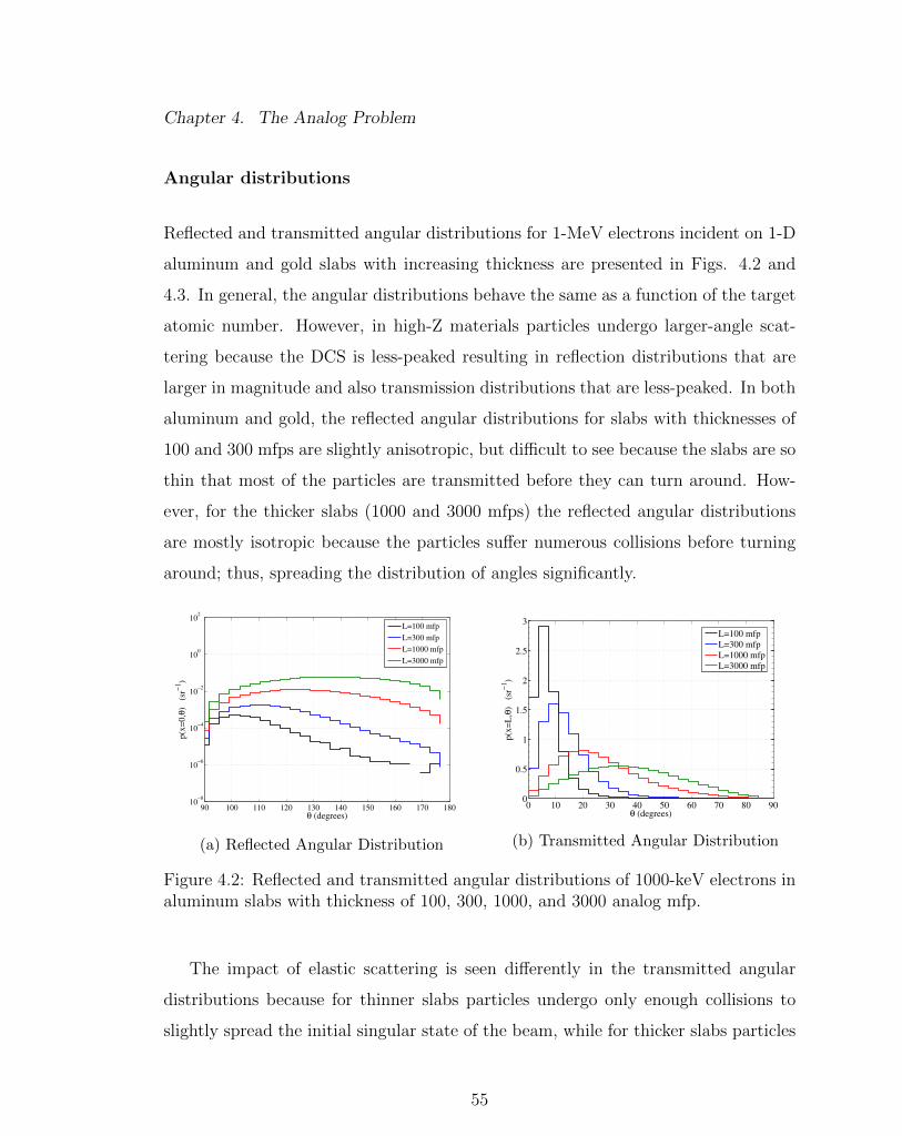
Chapter 4. The Analog Problem
Angular distributions
Reflected and transmitted angular distributions for 1-MeV electrons incident on 1-D
aluminum and gold slabs with increasing thickness are presented in Figs. 4.2 and
4.3. In general, the angular distributions behave the same as a function of the target
atomic number. However, in high-Z materials particles undergo larger-angle scat-
tering because the DCS is less-peaked resulting in reflection distributions that are
larger in magnitude and also transmission distributions that are less-peaked. In both
aluminum and gold, the reflected angular distributions for slabs with thicknesses of
100 and 300 mfps are slightly anisotropic, but difficult to see because the slabs are so
thin that most of the particles are transmitted before they can turn around. How-
ever, for the thicker slabs (1000 and 3000 mfps) the reflected angular distributions
are mostly isotropic because the particles suffer numerous collisions before turning
around; thus, spreading the distribution of angles significantly.
90 100 110 120 130 140 150 160 170 18010
−8
10−6
10−4
10−2
100
102
θ (degrees)
p(x
=0,θ
) (s
r−1)
L=100 mfp
L=300 mfp
L=1000 mfp
L=3000 mfp
(a) Reflected Angular Distribution
0 10 20 30 40 50 60 70 80 900
0.5
1
1.5
2
2.5
3
θ (degrees)
p(x
=L
,θ)
(s
r−1)
L=100 mfp
L=300 mfp
L=1000 mfp
L=3000 mfp
(b) Transmitted Angular Distribution
Figure 4.2: Reflected and transmitted angular distributions of 1000-keV electrons inaluminum slabs with thickness of 100, 300, 1000, and 3000 analog mfp.
The impact of elastic scattering is seen differently in the transmitted angular
distributions because for thinner slabs particles undergo only enough collisions to
slightly spread the initial singular state of the beam, while for thicker slabs particles
55

Chapter 4. The Analog Problem
90 100 110 120 130 140 150 160 170 180
10−4
10−2
100
102
θ (degrees)
p(x
=0,θ
) (s
r−1)
L=100
L=300
L=1000
L=3000
(a) Reflected Angular Distribution
0 10 20 30 40 50 60 70 80 900
0.5
1
1.5
2
θ (degrees)
p(x
=L
,θ)
(s
r−1)
L=100
L=300
L=1000
L=3000
(b) Transmitted Angular Distribution
Figure 4.3: Reflected and transmitted angular distributions of 1000-keV electrons ingold slabs with thickness of 100, 300, 1000, and 3000 analog mfp.
suffer enough collisions that the beam is spread out significantly from its initial state
resulting in a nearly isotropic distribution of angles.
Energy-loss spectra
Reflected and transmitted energy-loss spectra for 1-MeV electrons incident on 1-
D aluminum and gold slabs with increasing thickness are presented in Figs. 4.4
and 4.5. Once again, the overall behavior of the reflected and transmitted energy-
loss spectra is the roughly same as a function of the target atomic number. The
exception being that more particles are reflected in gold and the magnitude of the
reflected energy spectra are greater in gold, while the transmitted spectra are slightly
lower in magnitude. As the thickness of the slab increases, particles suffer further
inelastic collisions and the energy-loss spectra becomes smoother. This is true for
both reflected and transmitted energy-spectra.
56

Chapter 4. The Analog Problem
0 0.1 0.2 0.3 0.4 0.510
−6
10−4
10−2
100
E0−E (MeV)
p(0
,E0−
E)
(M
eV
−1)
L=100 mfp
L=300 mfp
L=1000 mfp
L=3000 mfp
(a) Reflected Energy-Loss Spectra
0 0.1 0.2 0.3 0.4 0.510
−6
10−4
10−2
100
102
104
E0−E (MeV)
p(L
,E0−
E)
(M
eV
−1)
L=100 mfp
L=300 mfp
L=1000 mfp
L=3000 mfp
(b) Transmitted Energy-Loss Spectra
Figure 4.4: Reflected and transmitted energy-loss spectra for 1000-keV electrons inaluminum slabs with thickness of 100, 300, 1000, and 3000 analog mfp.
Longitudinal and lateral distributions
Longitudinal and lateral distributions for 1-MeV electrons in an infinite copper
medium neglecting inelastic scattering are presented in Fig. 4.6. Longitudinal dis-
tributions give the displacement of the particle along the axis of the initial direc-
tion of the particle. This displacement is measured with respect to some maximum
pathlength and is therefore between −1 ≤ z/s ≤ 1 for longitudinal distributions.
As seen in Fig. 4.6a, for the thinnest slab (100 mfp) most particles stop between
0.95 < z/s ≤ 1 implying that after 100 collisions most particles are deflected incre-
mentally from their initial direction. However, it is clearly possible for the occasional
large angle scatter to result in particles traveling in directions opposite to their ini-
tial direction. As the slab thickens and particles suffer additional collisions, the
longitudinal distribution smoothes out.
Lateral distributions give the displacement of the particle perpendicular to the
axis of the initial direction of the particle. Again, this displacement is measured with
respect to some maximum pathlength, but is between 0 ≤ b/s ≤ 1 for lateral distri-
butions because this is essentially a measure of the radius of a beam. In Fig. 4.6b
57

Chapter 4. The Analog Problem
0 0.1 0.2 0.3 0.4 0.510
−6
10−4
10−2
100
102
E0−E (MeV)
p(0
,E0−
E)
(M
eV
−1)
L=100 mfp
L=300 mfp
L=1000 mfp
L=3000 mfp
(a) Reflected Energy-Loss Spectra
0 0.1 0.2 0.3 0.4 0.510
−6
10−4
10−2
100
102
104
E0−E (MeV)
p(L
,E0−
E)
(M
eV
−1)
L=100 mfp
L=300 mfp
L=1000 mfp
L=3000 mfp
(b) Transmitted Energy-Loss Spectra
Figure 4.5: Reflected and transmitted energy spectra for 1000-keV electrons in goldslabs with thickness of 100, 300, 1000, and 3000 analog mfp.
the lateral distributions appear to be smoother than the longitudinal distributions.
−1 −0.5 0 0.5 110
−6
10−4
10−2
100
102
z/s
P(z
/s)
s=100 mfp
s=300 mfp
s=1000 mfp
(a) Longitudinal Angular Distribution
0 0.2 0.4 0.6 0.8 110
−3
10−2
10−1
100
101
b/s
P(b
/s)
s=100 mfp
s=300 mfp
s=1000 mfp
(b) Lateral Distribution
Figure 4.6: Longitudinal and lateral distributions of 1000-keV electrons in gold slabswith thickness of 100, 300, and 1000 analog mfp.
Dose deposition
Depth-dose profiles for 20-MeV electrons normally incident on 30 cm of water and
250-keV electrons normally incident on 0.008 cm of gold are presented in Fig. 4.7 In
58
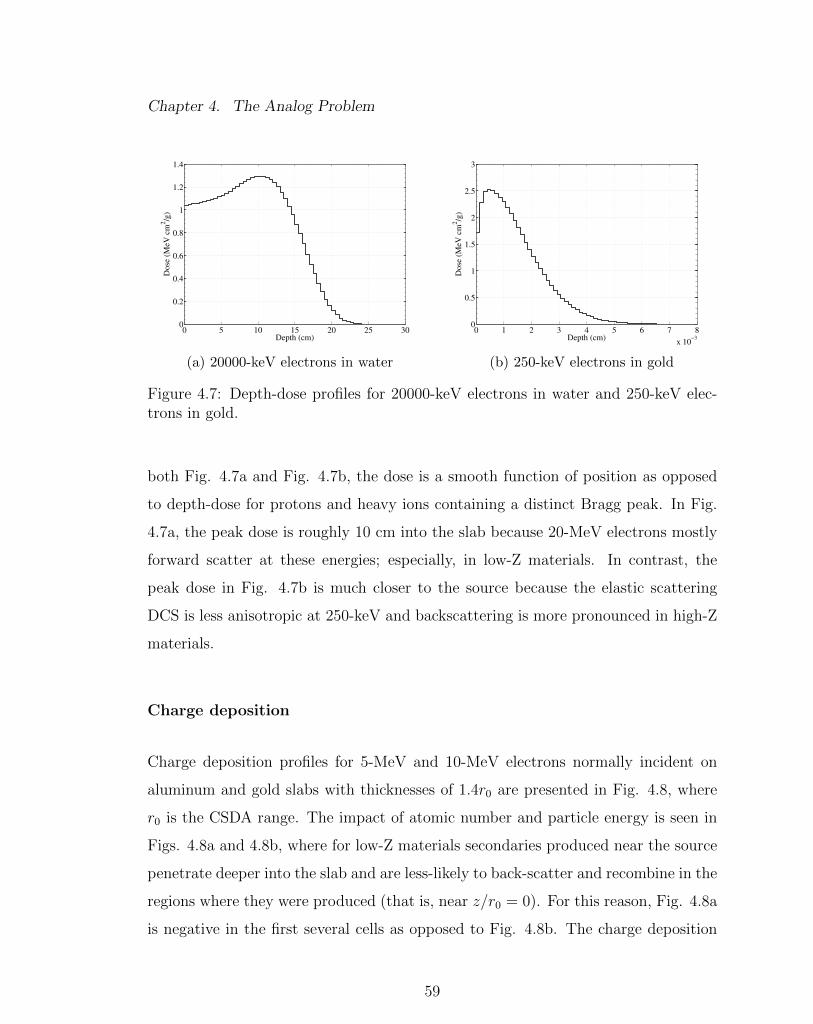
Chapter 4. The Analog Problem
0 5 10 15 20 25 300
0.2
0.4
0.6
0.8
1
1.2
1.4
Depth (cm)
Dose
(M
eV c
m2/g
)
(a) 20000-keV electrons in water
0 1 2 3 4 5 6 7 8
x 10−3
0
0.5
1
1.5
2
2.5
3
Depth (cm)
Dose
(M
eV
cm
2/g
)
(b) 250-keV electrons in gold
Figure 4.7: Depth-dose profiles for 20000-keV electrons in water and 250-keV elec-trons in gold.
both Fig. 4.7a and Fig. 4.7b, the dose is a smooth function of position as opposed
to depth-dose for protons and heavy ions containing a distinct Bragg peak. In Fig.
4.7a, the peak dose is roughly 10 cm into the slab because 20-MeV electrons mostly
forward scatter at these energies; especially, in low-Z materials. In contrast, the
peak dose in Fig. 4.7b is much closer to the source because the elastic scattering
DCS is less anisotropic at 250-keV and backscattering is more pronounced in high-Z
materials.
Charge deposition
Charge deposition profiles for 5-MeV and 10-MeV electrons normally incident on
aluminum and gold slabs with thicknesses of 1.4r0 are presented in Fig. 4.8, where
r0 is the CSDA range. The impact of atomic number and particle energy is seen in
Figs. 4.8a and 4.8b, where for low-Z materials secondaries produced near the source
penetrate deeper into the slab and are less-likely to back-scatter and recombine in the
regions where they were produced (that is, near z/r0 = 0). For this reason, Fig. 4.8a
is negative in the first several cells as opposed to Fig. 4.8b. The charge deposition
59

Chapter 4. The Analog Problem
0 0.2 0.4 0.6 0.8 1 1.2 1.4−1
−0.5
0
0.5
1
1.5
2
Scaled Depth (z/r0)
Scale
d C
harg
e D
eposi
tion (
r 0/e
)Dc
5000−keV
10000−keV
(a) Aluminum
0 0.2 0.4 0.6 0.8 1 1.2 1.4−0.5
0
0.5
1
1.5
2
2.5
Scaled Depth (z/r0)
Scale
d C
harg
e D
eposi
tion (
r 0/e
)Dc
5000−keV
10000−keV
(b) Gold
Figure 4.8: Charge deposition for 5000-keV and 10000-keV electrons in aluminumand gold.
profile in Fig. 4.8b is only slightly negative for 10-MeV electrons. In general, with
increasing source particle energy higher energy secondaries are produced carrying
dose further into the slab. As a result, the peak charge deposition is shifted deeper
into the slab.
Reflection and transmission fractions
Reflection and transmission fractions for 1-MeV electrons incident on 1-D aluminum
and gold slabs with increasing thickness are presented in Table 4.2. As expected,
nearly all of the electrons are transmitted in slabs with thicknesses of 100 to 300
mfps. However, with increasing thickness more particles are reflected; especially, in
gold as particles are more likely to back-scatter. Clearly, reflection and transmission
do not sum to one in all cases because some particles are absorbed in the slab.
60

Chapter 4. The Analog Problem
CEASE telescope response function calculation
The Compact Environmental Anomaly Sensor (CEASE) was built as a space parti-
cle radiation environment monitoring and warning system [1]. In particular, CEASE
monitors the radiation environment through measuring the energy spectra. In Fig.
4.9, the CEASE telescope is presented which is used to measure energy spectra.
The major components of the CEASE telescope include the collimator and the front
silicon detector (DFT) and the back silicon detector (DBT). Particles enter the tele-
scope through the collimator and deposit energy in both DFT and DBT. The energy
deposited in each detector is mapped to a channel determined according to the energy
deposition matrix in Fig. 4.10.
CEASE does not measure energy spectra directly, but rather measures raw counts
in response to electrons above ∼50-keV. To obtain energy spectra, one must relate
the raw counts to the spectra through the response function in the following integral
equation
Ci =
∫ ∞0
Ri(E)φ(E)dE, (4.48)
where Ci is the count rate (counts/sec.) for the ith channel, Ri(E) is the response
of the ith channel to particles with energy E, and φ(E) is the energy spectra. The
SlabThickness Material Reflection Transmission
100 mfpaluminum 0.0002±0.1 0.99979±0.00002
gold 0.003±0.02 0.99715±0.00005
300 mfpaluminum 0.0009±0.03 0.99964±0.00004
gold 0.017±0.007 0.9825±0.0001
1000 mfpaluminum 0.009±0.009 0.982±0.0001
gold 0.138±0.002 0.855±0.004
3000 mfpaluminum 0.041±0.005 0.701±0.001
gold 0.370±0.001 0.470±0.001
Table 4.2: Reflection and transmission fractions with relative uncertainties for 1-MeV electrons normally incident on aluminum and gold slabs with thicknesses of100, 300,1000, and 3000 mfps.
61

Chapter 4. The Analog Problem
Figure 4.9: Schematic of the CEASE telescope used to measure energy spectra [1].
response function (cm2sr),
Ri(E) = 2π
∫ θmax
0
Ai(E, θ) sin θdθ, (4.49)
is an integral of the effective area, Ai(E, θ), over all angles. The effective area is either
measured in the laboratory or calculated using a particle transport code. That is,
Ai(E, θ) =N iD(E, θ, εDFT , εDBT )
ρScos θ, (4.50)
where N iD(E, θ, εDFT , εDBT ) is the number of hits in the CEASE detector with energy
εDFT deposited in the front detector and εDBT deposited in the back detector, ρs = NsAs
is the source density, Ns is the total number of particles simulated, and AS is the
area of a disc source. Here, N iD(E, θ, εDFT , εDBT ) is calculated using a Monte Carlo
transport code and then some post-processing is used to carry out the integral in
Eq. (4.49).
62

Chapter 4. The Analog Problem
0.01 0.04 0.06 0.12 0.25 0.75 1.5 2.25 3 100.01
0.04
0.22
0.515
1.69
3.04
4.57
6.17.5
10
Front Detector Nominal Thresholds (MeV)
Back
Dete
cto
r N
om
inal
Th
resh
old
s (M
eV
) (5,4)
(5,5)
(0,3) (1,3)
(0,2) (1,2) (2,2) (3,2)
(0,1) (1,1) (2,1) (3,1) (5,1)
(0,0) (1,0) (2,0) (3,0) (5,0) (6,0) (8,0)
(8,1)
(8,2)
(8,3)
(8,4)
(4,0)
(4,1)
(4,2)
(4,3)
(4,4)
(4,5)
(3,3)(2,3)
Figure 4.10: CEASE telescope energy threshold matrix with channel labels [1].
In this section, the total response due to N channels or
R(E) = 2πN∑i=1
∫ θmax
0
Ai(E, θ) sin θdθ, (4.51)
is reported. To generate the total response, electrons with 62 different source energies
at 19 different source angles were simulated. The energy deposition matrix for each
source configuration was stored and processed. The result is given in Fig. 4.11. The
total response indicates the energy range for which the detector is responsive. An
ideal response is flat over all energies of interest. In Fig. 4.11, there is a lower energy
bound below which detector response is negligible and an upper energy bound above
which electrons fully penetrate the collimator and saturate the detector. To complete
a response function calculation 1116 different simulations were run with 30000 source
particles each. The total simulation time was 1380 processor-days. Of course, this
was divided among hundreds of cores making the computational cost manageable.
63
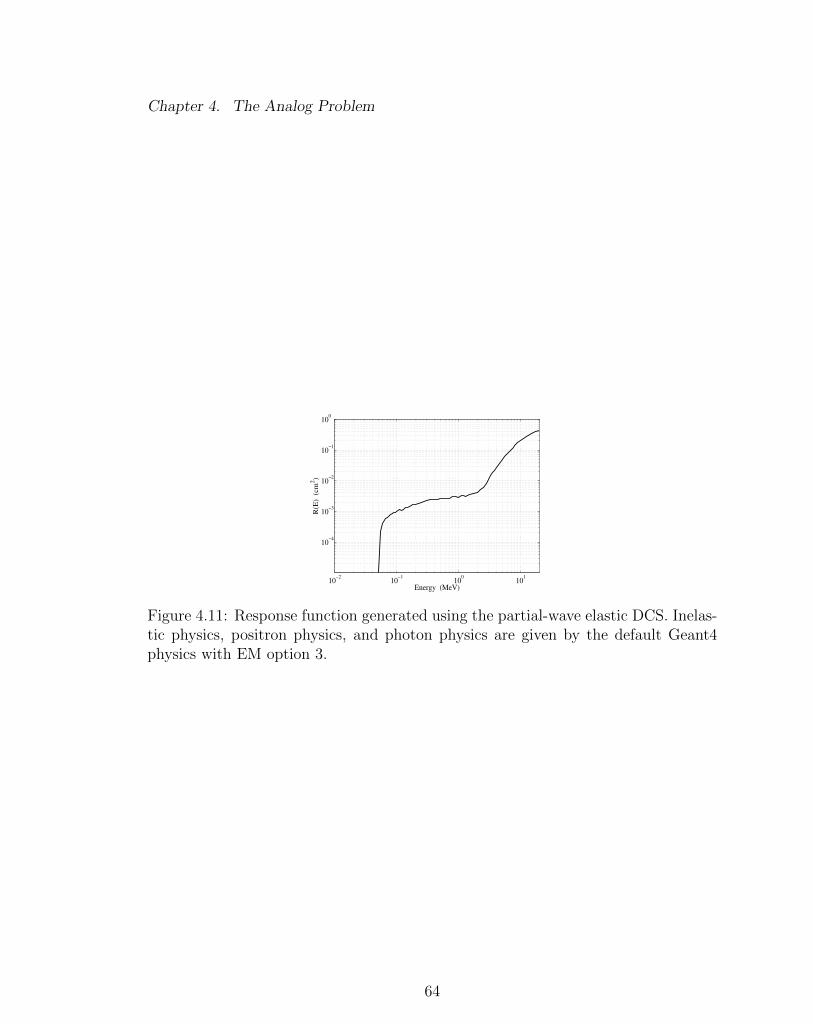
Chapter 4. The Analog Problem
10−2
10−1
100
101
10−4
10−3
10−2
10−1
100
Energy (MeV)
R(E
) (
cm
2)
Figure 4.11: Response function generated using the partial-wave elastic DCS. Inelas-tic physics, positron physics, and photon physics are given by the default Geant4physics with EM option 3.
64

Chapter 5
Differential Cross-Section
Moments
In this chapter, the concept of a mathematical moment is developed. Given a general
understanding of the information contained in a moment, the elastic and inelastic
moments are again defined. With these definitions, the importance of moments
within the context of electron transport is demonstrated. As previously discussed
(see Chapter 3), it is possible to understand the importance of the lowest order
moments through their physical interpretation. However, beyond low order moments
it is difficult to make a physical connection; therefore, we must rely on mathematical
interpretations where physical interpretations are not possible.
In mathematics, a moment is a specific quantitative measure of the shape of a
set of points used in statistics. Moreover, one can reconstruct a distribution given
the information contained in the moments of that distribution. Take for example the
normal distribution or
f(x, µ, σ) =1
σ√
2πe−
(x−µ)2
2σ2 , (5.1)
where µ is the mean and σ2 is the variance as seen in Fig. 5.1. A normal distribution
65

Chapter 5. Differential Cross-Section Moments
Figure 5.1: The normal distribution.
is completely specified by the mean, µ, and the variance, σ2.
The role of moments is perhaps easier to understand in a mathematical context. It
is then possible to extend these ideas to understanding the importance of moments
of the analog DCS. To begin, the central moments, or moments of a probability
distribution about the mean, are given by
µn =
∫ ∞−∞
(x− µ)nf(x)dx. (5.2)
Given the definition of the normal distribution and the central moments, the zeroth
moment (n = 0) is defined. The zeroth moment gives the total area under a curve. By
definition, all probability distributions are normalized such that the zeroth moment
is unity. Therefore, the zeroth moment of the normal distribution is
µ0 =
∫ ∞−∞
1
σ√
2πe−
(x−µ)2
2σ2 dx = 1. (5.3)
In words, the zeroth moment is the probability that any possible outcome will occur
and, therefore, must be one. The first central moment or the mean is given by
µ1 = µ =
∫ ∞−∞
(x− µ)1
σ√
2πe−
(x−µ)2
2σ2 dx. (5.4)
The mean provides the central tendency of a probability distribution and because
the normal distribution is symmetric, the distribution is centered about the mean.
66

Chapter 5. Differential Cross-Section Moments
The second central moment or the variance is given by
µ2 = σ2 =
∫ ∞−∞
(x− µ)2 1
σ√
2πe−
(x−µ)2
2σ2 dx (5.5)
and provides a measure of the width of the distribution. As described by Eq. (5.1),
the normal distribution can be reconstructed with the mean and the variance or the
first and second moments. The third central moment or the skewness is given by
µ3 =
∫ ∞−∞
(x− µ)3 1
σ√
2πe−
(x−µ)2
2σ2 dx = 0, (5.6)
and is, of course, zero because the normal distribution is symmetric. The forth
central moment or the kurtosis is given by
µ4 =
∫ ∞−∞
(x− µ)4 1
σ√
2πe−
(x−µ)2
2σ2 dx = 3σ4, (5.7)
and is a measure of whether a distribution is tall and skinny or short and squat.
Higher-order moments, beyond kurtosis or the fourth central moment, are generally
interpreted as estimations of further shape parameters used to capture a distribution.
However, it is difficult to describe exactly how these higher order terms impact a
distribution. That is not to say that these moments can simply be neglected or do
not play an important role.
Observations similar to those made of moments of the normal distribution can be
extended to electron transport and the physics associated with elastic and inelastic
scattering. In general, the moments with clear physical interpretations include the
zeroth, first, and second moments, which are referred to as the total cross-section
(elastic and inelastic), the transport cross-section or the mean scattering angle (elas-
tic), the stopping power or the mean energy-loss per unit distance (inelastic), the
mean-square scattering angle (elastic), and energy straggling or the mean-square
energy-loss (inelastic).
67
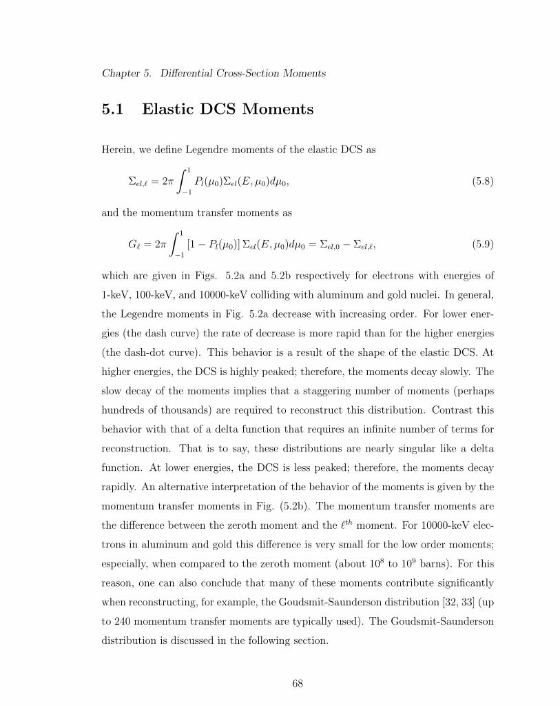
Chapter 5. Differential Cross-Section Moments
5.1 Elastic DCS Moments
Herein, we define Legendre moments of the elastic DCS as
Σel,` = 2π
∫ 1
−1
Pl(µ0)Σel(E, µ0)dµ0, (5.8)
and the momentum transfer moments as
G` = 2π
∫ 1
−1
[1− Pl(µ0)] Σel(E, µ0)dµ0 = Σel,0 − Σel,`, (5.9)
which are given in Figs. 5.2a and 5.2b respectively for electrons with energies of
1-keV, 100-keV, and 10000-keV colliding with aluminum and gold nuclei. In general,
the Legendre moments in Fig. 5.2a decrease with increasing order. For lower ener-
gies (the dash curve) the rate of decrease is more rapid than for the higher energies
(the dash-dot curve). This behavior is a result of the shape of the elastic DCS. At
higher energies, the DCS is highly peaked; therefore, the moments decay slowly. The
slow decay of the moments implies that a staggering number of moments (perhaps
hundreds of thousands) are required to reconstruct this distribution. Contrast this
behavior with that of a delta function that requires an infinite number of terms for
reconstruction. That is to say, these distributions are nearly singular like a delta
function. At lower energies, the DCS is less peaked; therefore, the moments decay
rapidly. An alternative interpretation of the behavior of the moments is given by the
momentum transfer moments in Fig. (5.2b). The momentum transfer moments are
the difference between the zeroth moment and the `th moment. For 10000-keV elec-
trons in aluminum and gold this difference is very small for the low order moments;
especially, when compared to the zeroth moment (about 108 to 109 barns). For this
reason, one can also conclude that many of these moments contribute significantly
when reconstructing, for example, the Goudsmit-Saunderson distribution [32, 33] (up
to 240 momentum transfer moments are typically used). The Goudsmit-Saunderson
distribution is discussed in the following section.
68

Chapter 5. Differential Cross-Section Moments
0 5 10 15 20 25 3010
7
108
109
1010
1011
1012
Order
Ml (
barn
s)
1−keV, Al
100−keV, Al
10000−keV, Al
1−keV, Au
100−keV, Au
10000−keV, Au
(a) Legendre Moments
5 10 15 20 25 30
100
102
104
106
108
1010
Order
Gl (
barn
s)
1−keV, Al
100−keV, Al
10000−keV, Al
1−keV, Au
100−keV, Au
10000−keV, Au
(b) Momentum Transfer Moments
Figure 5.2: Legendre moments and momentum transfer moments of the Partial-wavedifferential cross-section for elastic collisions with aluminum and gold nuclei..
5.2 Inlastic DCS Moments
Herein, we define energy-loss moments of the inelastic DCS as
Qk =
∫ Qmax
Qmin
QkΣin(E,Q)dQ. (5.10)
The first seven energy-loss moments are given in Fig. 5.3 as a function of energy.
At lower energies, the moments appear to decay; however, energy-loss moments are
asymptotic. That is, beyond a specific order for all energies, the moments begin to
grow without bound, which is clear in Fig. 5.3 at higher energies where the higher-
order moments begin to grow larger than the lower order moments. This implies
that for higher energies the higher-order moments are more important than for lower
energies. In fact, for energies greater than roughly 7-MeV, the straggling coefficient
Q2 is as large as the stopping power Q1, which would imply that these processes
contribute equally at these energies. In other words, at higher energies particles
suffer numerous collisions resulting in small energy losses, which can be described by
the continuous slowing down approximation through the stopping power. However,
occasional large energy losses do occur that contribute significantly to the solution.
69
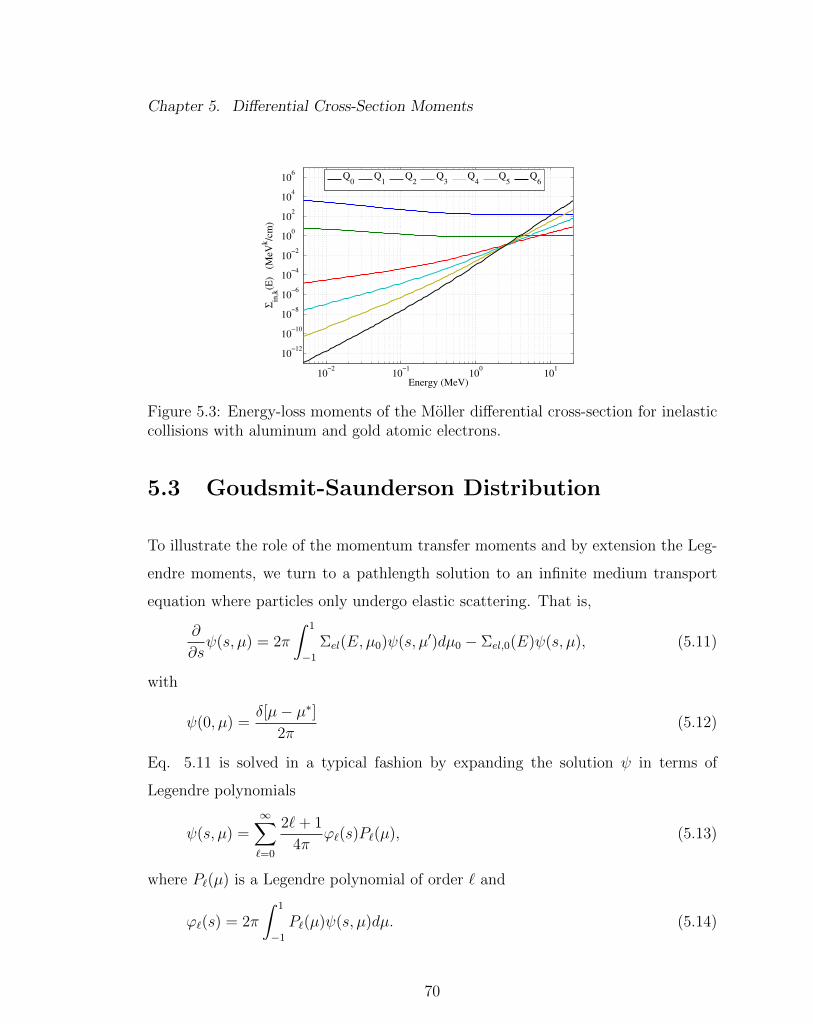
Chapter 5. Differential Cross-Section Moments
10−2
10−1
100
101
10−12
10−10
10−8
10−6
10−4
10−2
100
102
104
106
Energy (MeV)
Σin
,k(E
) (M
eV
k/c
m)
Q
0Q
1Q
2Q
3Q
4Q
5Q
6
Figure 5.3: Energy-loss moments of the Moller differential cross-section for inelasticcollisions with aluminum and gold atomic electrons.
5.3 Goudsmit-Saunderson Distribution
To illustrate the role of the momentum transfer moments and by extension the Leg-
endre moments, we turn to a pathlength solution to an infinite medium transport
equation where particles only undergo elastic scattering. That is,
∂
∂sψ(s, µ) = 2π
∫ 1
−1
Σel(E, µ0)ψ(s, µ′)dµ0 − Σel,0(E)ψ(s, µ), (5.11)
with
ψ(0, µ) =δ[µ− µ∗]
2π(5.12)
Eq. 5.11 is solved in a typical fashion by expanding the solution ψ in terms of
Legendre polynomials
ψ(s, µ) =∞∑`=0
2`+ 1
4πϕ`(s)P`(µ), (5.13)
where P`(µ) is a Legendre polynomial of order ` and
ϕ`(s) = 2π
∫ 1
−1
P`(µ)ψ(s, µ)dµ. (5.14)
70
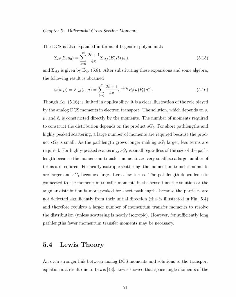
Chapter 5. Differential Cross-Section Moments
The DCS is also expanded in terms of Legendre polynomials
Σel(E, µ0) =∞∑`=0
2`+ 1
4πΣel,`(E)P`(µ0), (5.15)
and Σel,` is given by Eq. (5.8). After substituting these expansions and some algebra,
the following result is obtained
ψ(s, µ) = FGS(s, µ) =∞∑`=0
2`+ 1
4πe−sG`P`(µ)P`(µ
∗). (5.16)
Though Eq. (5.16) is limited in applicability, it is a clear illustration of the role played
by the analog DCS moments in electron transport. The solution, which depends on s,
µ, and `, is constructed directly by the moments. The number of moments required
to construct the distribution depends on the product sG`. For short pathlengths and
highly peaked scattering, a large number of moments are required because the prod-
uct sG` is small. As the pathlength grows longer making sG` larger, less terms are
required. For highly-peaked scattering, sG` is small regardless of the size of the path-
length because the momentum-transfer moments are very small, so a large number of
terms are required. For nearly isotropic scattering, the momentum-transfer moments
are larger and sG` becomes large after a few terms. The pathlength dependence is
connected to the momentum-transfer moments in the sense that the solution or the
angular distribution is more peaked for short pathlengths because the particles are
not deflected significantly from their initial direction (this is illustrated in Fig. 5.4)
and therefore requires a larger number of momentum transfer moments to resolve
the distribution (unless scattering is nearly isotropic). However, for sufficiently long
pathlengths fewer momentum transfer moments may be necessary.
5.4 Lewis Theory
An even stronger link between analog DCS moments and solutions to the transport
equation is a result due to Lewis [43]. Lewis showed that space-angle moments of the
71
Chapter 5. Differential Cross-Section Moments
Figure 5.4: Hypothetical paths traveled by electrons.
solution only depend on momentum transfer moments of the analog DCS. In other
words, Lewis theory is a statement of equivalence between preservation of space-
angle moments of the solution and Legendre moments of the analog DCS. Here this
result is derived in 1-D to illustrate the relationship between space-angle moments
of solutions to the transport equation and Legendre moments of the analog DCS for
elastic scattering.
We begin by writing down an infinite homogeneous medium transport equation
in 1-D, planar geometry for mono-energetic electrons or
∂
∂sψ(s, z, µ)+µ
∂
∂zψ(z, z, µ) = 2π
∫ 1
−1
Σel(E, µ0)ψ(s, z, µ′)dµ0−Σel,0(E)ψ(s, z, µ),
(5.17)
with the following initial condition
ψ(0, z, µ) = δ(z)δ(µ− 1)
2π(5.18)
We then define spatial moments of the solution as
ϕn =
∫ ∞−∞
dz znψ(s, z, µ). (5.19)
If we take zn moments of Eq. 5.17, we have
∂
∂sϕn(s, µ)−µϕn−1(s, µ) = 2π
∫ 1
−1
Σel(E, µ0)ϕn(s, µ)dµ0−Σel,0(E)ϕn(s, µ), (5.20)
72
Chapter 5. Differential Cross-Section Moments
with
ϕn(0, µ) = δn0δ(µ− 1)
2π. (5.21)
We now define mixed spatial and Legendre moments of the solution as
ϕmn = 2π
∫ 1
−1
dµ
∫ ∞−∞
dz znPm(µ)ψ(s, z, µ), (5.22)
expand the elastic DCS
Σel(E, µ0) =∞∑`=0
2`+ 1
4πΣel,`P`(µ
′)P`(µ), (5.23)
and take Legendre moments of Eq. (5.20) which gives
∂
∂sϕnm(s) + Σel,0(E)ϕnm(s, µ) = Σel,`ϕnm(s) + 2π
∫ 1
−1
µPm(µ)ϕn−1(s, µ). (5.24)
Rearranging Eq. (5.24) and using properties of Legendre polynomials to expand
µPm(µ) gives
∂
∂sϕnm(s)+Gmϕnm(s, µ) = n
[m
2m+ 1ϕn−1,m−1(s) +
m+ 1
2m+ 1ϕn−1,m+1(s)
], (5.25)
for n,m = 0, 1, 2, ..., where φnm(0) = δn0. The general solution to Eq. (5.25) is
ϕmn(S) = δn0e−sGm+n
∫ s
0
ds′e−Gm(s−s′)[
m
2m+ 1ϕn−1,m−1(s′) +
m+ 1
2m+ 1ϕn−1,m+1(s′)
].
(5.26)
One cannot obtain a solution to Eq. (5.17) given the Lewis moments. One can
show that the mixed spatial and Legendre moments of the solution, which can be
related to space-angle moments of the solution, only depend on Gm. This relationship
is the important result from Lewis theory. To do so, we begin by setting n = 0 which
gives
ϕm0(S) = e−sGm . (5.27)
73
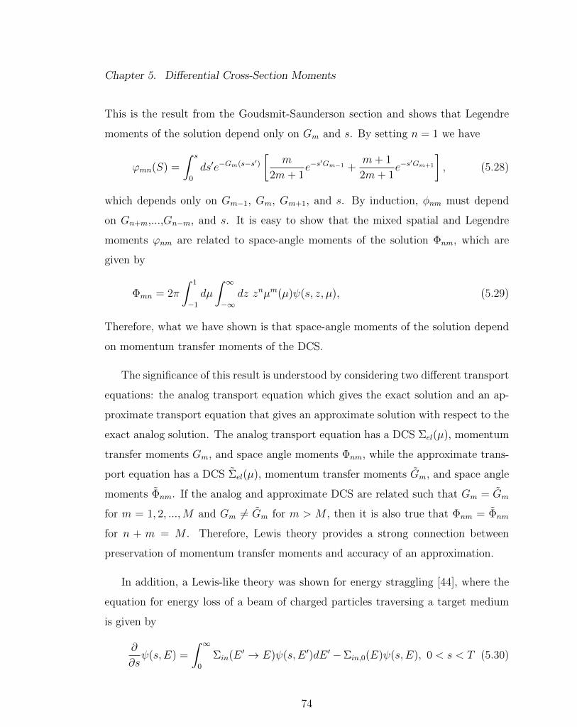
Chapter 5. Differential Cross-Section Moments
This is the result from the Goudsmit-Saunderson section and shows that Legendre
moments of the solution depend only on Gm and s. By setting n = 1 we have
ϕmn(S) =
∫ s
0
ds′e−Gm(s−s′)[
m
2m+ 1e−s
′Gm−1 +m+ 1
2m+ 1e−s
′Gm+1
], (5.28)
which depends only on Gm−1, Gm, Gm+1, and s. By induction, φnm must depend
on Gn+m,...,Gn−m, and s. It is easy to show that the mixed spatial and Legendre
moments ϕnm are related to space-angle moments of the solution Φnm, which are
given by
Φmn = 2π
∫ 1
−1
dµ
∫ ∞−∞
dz znµm(µ)ψ(s, z, µ), (5.29)
Therefore, what we have shown is that space-angle moments of the solution depend
on momentum transfer moments of the DCS.
The significance of this result is understood by considering two different transport
equations: the analog transport equation which gives the exact solution and an ap-
proximate transport equation that gives an approximate solution with respect to the
exact analog solution. The analog transport equation has a DCS Σel(µ), momentum
transfer moments Gm, and space angle moments Φnm, while the approximate trans-
port equation has a DCS Σel(µ), momentum transfer moments Gm, and space angle
moments Φnm. If the analog and approximate DCS are related such that Gm = Gm
for m = 1, 2, ...,M and Gm 6= Gm for m > M , then it is also true that Φnm = Φnm
for n + m = M . Therefore, Lewis theory provides a strong connection between
preservation of momentum transfer moments and accuracy of an approximation.
In addition, a Lewis-like theory was shown for energy straggling [44], where the
equation for energy loss of a beam of charged particles traversing a target medium
is given by
∂
∂sψ(s, E) =
∫ ∞0
Σin(E ′ → E)ψ(s, E ′)dE ′−Σin,0(E)ψ(s, E), 0 < s < T (5.30)
74
Chapter 5. Differential Cross-Section Moments
with initial condition
ψ(0, E) = δ[E0 − E]. (5.31)
In Eq. (5.30), s is the distance travelled by a particle, E is the particle energy,
ψ(s, E) is the solution or the energy spectrum, and Σin and Σin,0 are the DCS and
total cross-section respectively. Similar to obtaining the result from Lewis theory,
we define energy moments of the solution as
Ik(s) =
∫ ∞0
Ekψ(s, E)dE, (5.32)
and then relate these moments to the energy-loss moments from Eq. (3.38). The
resulting theorem states that if the energy-loss moments from Eq. (3.38) for the
analog and approximate problem satisfy Qk = Qk for k = 1, 2, ..., K for some finite
K then ψ(S,E) is an N th-order moment-preserving approximation to ψ(s, E) in the
sense that∫ ∞0
Ek[ψ(s, E)− ψ(s, E)]dE = 0, n = 1, 2, ..., N (5.33)
where ψ(s, E) is the approximate solution with an approximate DCS Σel(E′ → E).
5.5 Eigenvalues of the Elastic Collision Operator
Eigenvalues have a wide variety of applications. In the context of operators, eigen-
values can be used to characterize or understand the properties of an operator. For
elastic collision operator, one finds that the eigenvalues are bounded, therefore, the
operator is stable. Moreover, it of interest to develop approximate operators and
one can get a sense of the accuracy of an approximate operator by comparing the
eigenvalues of the approximation to the eigenvalues of true operator. That said, the
eigenvalues of the elastic collision operator are related to the moments of the elastic
75
Chapter 5. Differential Cross-Section Moments
DCS. Therefore, in a completely different context, yet again we see the necessity of
moment-preservation. To be clear, we derive an expression for the eigenvalues of the
elastic collision operator given by
Helψ = 2π
∫ 1
−1
dµ′Σel(E, µ0)ψ(E, µ′)− Σel,0(E)ψ(E, µ) = λψ(E, µ). (5.34)
We begin by defining Legendre moments of the solution as
ϕ`(E) = 2π
∫ 1
−1
dµP`(µ)ψ(E, µ), (5.35)
and expand the DCS in term of Legendre polynomials
Σel(E, µ0) =∞∑`=0
2`+ 1
4πΣel,`P`(µ
′)P`(µ). (5.36)
Now, Eq. (5.36) is substituted into Eq. (5.34) and the left-hand side is rearranged
such that Eq. (5.35) can be substituted or
λψ(E, µ) =∞∑`=0
2`+ 1
2Σel,`P`(µ)
∫ 1
−1
dµ′P`ψ(E, µ′)− Σel,0(E)ψ(E, µ). (5.37)
We then apply orthogonality
2π
∫ 1
−1
dµPm(µ)
[λψ(E, µ) =
∞∑`=0
2`+ 1
2Σel,`P`(µ)ϕ`(E)− Σel,0(E)ψ(E, µ)
], (5.38)
and obtain
λmϕm(E) = − [Σel,0(E)− Σel,m(E)]ϕm(E), (5.39)
In Eq. (5.39),
λm = − [Σel,0(E)− Σel,m(E)] (5.40)
are the eigenvalues and equal to the momentum-transfer moments defined by Eq.
(5.9) (presented in Fig. 5.2b) and ϕm(E) are the associated eigenfunctions. Now if
one were to obtain an approximation to Eq. (5.34), a comparison of the eigenval-
ues of the approximate and exact operator provides a measure the accuracy of the
76

Chapter 5. Differential Cross-Section Moments
approximation. Moreover, if one were to simply approximate the DCS and, in turn,
the operator, then one must ensure that the approximate DCS preserves as many
moments of the analog DCS as reasonably possible. That said, the accuracy of the
approximate operator is difficult to measure irrespective of the problem to which the
operator is applied. That is, when calculating dose in thick targets, one can expect
to reasonably approximate the elastic collision operator with an operator that only
preserves a relatively small number of eigenvalues. However, calculating differential
distributions in angle in thin targets may require preservation of a large number of
eigenvalues.
A similar analysis for the inelastic collision operator is not possible because it is
not possible to determine the eigenvalues of this operator. However, the Lewis-theory
for energy straggling is sufficient to suggest that an accurate approximate inelastic
operator consists of a moment-preserving scattering kernel.
77
Chapter 6
The Condensed History Method
In this chapter, the condensed history (CH) method for electron transport is re-
viewed. This includes an introduction to the CH method, an outline of the CH class
I and class II algorithms and the limitations associated with these schemes.
Berger describes CH as an alternative approach to direct simulation of Coulomb
scattering, in which the diffusion process is imitated by letting the particles carry out
an (artificially constructed) random walk, each step of which takes into account the
combined effect of many collisions [2]. This artificially constructed random walk is
typically referred to as a step and on the order of hundreds of analog mfps making the
calculation more efficient. However, by extending the distances between collisions to
a step-size, the analog DCS is no longer valid. Therefore, one typically replaces the
DCSs with the corresponding multiple scattering and energy-loss straggling theories
that are solutions to transport equations requiring severe restrictions necessary for
analytical treatment. That is, without making simplifying assumptions it would be
impossible to obtain a useful solution to the transport equation. Use of multiple
scattering and energy-loss straggling distributions rather than a DCS, in effect, re-
quires an operator split procedure [39], where one is now approximating the solution
78

Chapter 6. The Condensed History Method
to the transport equation.
As a result of applying multiple scattering and energy-loss straggling distributions
and the operator split procedure, CH suffers from inherent limitations. In partic-
ular, these limitations are due to application of multiple scattering and energy-loss
straggling distributions outside of the conditions for which multiple scattering and
energy-loss straggling theory is valid and a deterministic error resulting from the
operator split procedure necessary to utilize multiple scattering theory. These limi-
tations are a result of some or all of the following assumptions required for analytical
treatment:
• infinite medium;
• negligible energy-loss;
• negligible angular deflection;
• small-angle approximation;
• no spatial correlation.
Some specific examples of commonly used multiple scattering and energy-loss strag-
gling theory and the associated limitations are now provided.
First, multiple scattering theories due to Moliere [66] and Goudsmit-Saunderson
[32, 33] are discussed. The Moliere distribution is typically found in CH algorithms
where multiple-scattering distributions are required for randomly sampled steps. The
form of the Moliere distribution, a universal function of a scaled angular variable,
makes it ideal for such CH algorithms. However, the small-angle approximation is
required to obtain the Moliere distribution and is limited to deflections of no more
than about 20 degrees. In addition, spin and relativistic effects are not taken into ac-
count and the distribution is restricted to at least roughly 100 elastic collisions, which
79
Chapter 6. The Condensed History Method
can be difficult to satisfy with the CH algorithm [71]. The Goudsmit-Saunderson
distribution is more complicated for sampling purposes, but it is not restricted by
the small-angle approximation and in theory, it is not restricted to steps of at least
roughly 100 elastic collisions1. Also, the Goudsmit-Saunderson distribution can be
applied to any DCS for which moments up to an arbitrary order can be generated.
However, this all comes at a price because the Goudsmit-Saunderson distribution
must be stored for predetermined steps because it is impractical to apply to randomly
sampled steps. Ultimately, this results in a significantly different CH algorithm from
the CH algorithm associated with the Moliere distribution. Regardless of the type
of multiple-scattering distribution, the distributions are only valid for an infinite
medium and though one can account for energy dependence through the CSDA, this
solution does not provide any information about the distribution of energies after a
step. Therefore, the multiple-scattering distributions are limited to angular informa-
tion for particles with steps s in an infinite medium where energy-loss is, at most,
accounted for in a CSD fashion. Furthermore, space-angle correlations are not di-
rectly accounted for in multiple-scattering distributions, so when a particle is forced
to travel a distance s in a straight path some error in the longitudinal and lateral
displacement is incurred.
Another example includes the Landau distribution for multiple excitations and
ionizations [34] or energy-loss straggling. The Landau distribution, accounts for the
energy lost after traveling a distance s. However, Landau theory takes into account
only the mean value, but not the higher moments, of the cross section for small
energy transfers [71]. The Blunck-Leisegang correction [72] takes into account the
correct second moment and consists of convoluting the Landau distribution with a
Gaussian distribution with a zero mean value and with the appropriate variance [71].
Even then, the “appropriate” variance is not necessarily a straightforward quantity
1In practice, the numerics required to generate the Goudsmit-Saunderson distribution strugglewith sufficiently small steps [42]
80
Chapter 6. The Condensed History Method
and there are various procedures for estimating it. As a result of the condition for the
applicability of Landau theory, the step-size is required to be longer than desirable
for the sampling of the multiple elastic scattering distributions. In addition, by
extending the distance traveled by an electron, secondary production is no longer
sampled directly and must be accounted on an average basis. As an alternative
to Landau theory, it is possible to separate inelastic collisions into “soft” collisions
(with large impact parameters2 and small momentum transfers and energy losses)
and “hard” collisions (with small impact parameters and large momentum transfers
and energy losses). Typically, an energy cut-off is selected below which collisions are
considered soft and the CSDA is applied. Above the cut-off collisions are considered
hard and an inelastic DCS is used to sample energy loss and subsequent secondary
production. With this treatment, secondary production is captured exactly and
random sampling of steps is possible.
Given the multiple-scattering and energy-loss straggling theories, which are ap-
proximate, CH combines the necessary theories into one coherent scheme. The
multiple-scattering and energy-loss straggling distributions are typically smoother
and less peaked than the analog DCS. This feature combined with the fact that a
step is typically hundreds of analog mfps leads to a more efficient calculation. Dif-
ferent combinations of different multiple-scattering and energy-loss straggling dis-
tributions results in different CH schemes. There are two major schemes, class I
and class II, and the major distinction between the two is whether particles move
fixed, deterministic steps or randomly sampled steps. An example of the class I
CH scheme is the ITS code system [73], where particles move a fixed step-size and
elastic and inelastic collisions are given by the Goudsmit-Saunderson and Landau
distributions respectively. An example of the class II CH scheme is the EGS code
system, where the step-size is chosen as the minimum of the distance in the current
2The impact parameter characterizes the “closeness” of the collision. Closer collisions with smallimpact parameters are more catastrophic.
81

Chapter 6. The Condensed History Method
direction to the nearest boundary, the exponentially distributed distance associated
with sampling distance to hard collisions, and the maximum step-size for which
the multiple-scattering theory is valid. In EGS, elastic collisions are given by the
Moliere distribution and inelastic collisions separated into soft and hard collisions.
Regardless of the CH scheme, the application of multiple-scattering and energy-loss
straggling theory results in limitations that impact the accuracy of the CH method.
In particular, the accuracy of CH is step-size dependent even when applied to an
infinite medium problem [39]. Moreover, when applying multiple-scattering theory
in a heterogenous media, additional error is introduced at material interfaces because
multiple-scattering distributions are typically valid for an infinite medium. In both
class I and class II CH schemes, it is possible to mitigate the impact of the aforemen-
tioned limitations by introducing algorithms that determine the optimal step-sizes
or perform tedious studies for the same purpose.
In the remaining sections, the CH algorithm is discussed and the class I and
class II schemes are outlined. Given an understanding of the CH algorithm, the
aforementioned limitations are discussed in greater detail along with a demonstration
of the typical approaches for mitigating these limitations.
6.1 The Condensed History Algorithm
In this section, the class I and class II condensed history schemes are discussed. In
particular, the class I scheme discussed is based on the ITS algorithm, while the
class II scheme discussed is based on the Geant4 algorithm. The descriptions of
the algorithms are intended to emphasize the differences between the two schemes
and are not necessarily perfect descriptions. To fully understand the two different
algorithms, one should refer to the manuals and the source code (where possible) for
both code systems [73, 3].
82

Chapter 6. The Condensed History Method
6.1.1 Complete grouping, class I
Class I CH algorithms have the oldest history of the different schemes and date back
to the original ETRAN code system [16]. One might argue that the distinguish-
ing feature of class I algorithms is the treatment of secondaries, or perhaps, fixed
step-sizes resulting from use of the Goudsmit-Saunderson distribution3. Regardless,
the resulting algorithm is the same. That is, if one decides to use the Goudsmit-
Saunderson distribution for fixed step-sizes, a mixed approach for energy-loss strag-
gling is no longer appropriate. Therefore, Landau theory is used and secondaries are
treated on an average basis. Alternatively, one could decide to use Landau theory
and as a result, would be forced to handle secondary production accordingly making
use of fixed step-sizes and the Goudsmit-Saunderson distribution a natural choice.
That said, class I algorithms move electrons fixed distances over which the electron is
assumed to lose a constant fraction of energy (typically about 8%). An energy grid is
established for corresponding to this fractional energy loss and step-sizes consistent
with the energy grid are determined. Multiple-scattering and energy-loss straggling
distributions are also pre-computed and stored for the previously mentioned energy
grid. Once the pre-processing is completed electrons are transported according to
the design of the algorithm specific to the code system. The remainder of this section
presents an overview of an ITS-like algorithm.
To begin, the data for the simulation must be prepared. For electrons, this
includes generating multiple-scattering and energy-loss straggling distributions for
an energy grid determined by the maximum particle energy and the cut-off energy.
The energy grid is determined by the following expression
Ek = Ek−12−1/J , (6.1)
where J is typically set to 8. Now, steps are generated for the K − 1 energy-losses,
3There are codes that now use Goudsmit-Saunderson for randomy sampled step-sizes [?].
83

Chapter 6. The Condensed History Method
or ∆Ek = Ek − Ek−1. The Landau distribution is evaluated at each of the k energy
grid points along with the Goudsmit-Saunderson distribution where some effort is
made to account for the changing energy over the step. The steps are sub-divided
into m sub-steps. This is, of course, executed for all materials. Given the necessary
data, the transport begins.
First, energy-straggling is determined for the entire step. Once the energy loss
for the step is determined it is applied in a CSD manner divided evenly among the
sub-steps in the step [74]. The electron is moved the distance of a sub-step and at
this point, angular deflection is sampled from the Goudsmit-Saunderson distribution
and secondaries are sampled. Secondaries are sampled based on the mean number
expected to be produced above the cut-off energy over the sub-step distance. The
mean number expected is determined by integrating the Moller DCS over the range
above the cut-off energy and dividing the sub-step by this quantity. The energies of
the secondaries are also sampled from the Moller DCS above the cut-off. Given the
mean expected secondary production and their energies, the locations of the secon-
daries are sampled randomly along the sub-step. It is important to note that the
energy lost by the primary electron is accounted for at the beginning of the step.
When secondaries are produced negative energy deposition is tallied to account for
the removal of energy in the form of a secondary. Though negative energy deposi-
tion is non-physical, energy balance is achieved over many histories. bremsstrahlung
photons are also produced over a sub-step and sampled from the Poisson distribu-
tion. However, the energy of the primary electron is reduced by the energy of the
bremsstrahlung photons produced along the sub-step because photon production is
not accounted for in the energy-loss straggling. The process of moving a particle over
a sub-step is repeated until the particle reaches the end of the step. At this point,
the energy-loss straggling distribution is again sampled and all of the processes at
the sub-step level are repeated.
84
Chapter 6. The Condensed History Method
The process of transporting the electron is interrupted when a material boundary
is encountered. This is a complication for the algorithm because the sub-step must
be truncated at the boundary and the multiple scattering distributions are prede-
termined for fixed steps. Therefore, a modified multiple-scattering distribution, or
the Jordan-Mack correction, is applied [41]. This distribution takes the form of
a Gaussian to account for small-angle scatter plus a Poisson to account for large-
angle scatter. The distribution is applied over the truncated sub-step. Secondary
production and bremsstrahlung photons are determined as usual for the truncated
step. However, the energy-loss straggling that was calculated for the entire step must
now be corrected for the abbreviated step. This is done by re-sampling the Landau
distribution for the abbreviated step.
Once the particle leaves the problem volume or slows down through the minimum
energy, the particle is killed and a new history begins.
6.1.2 Mixed procedures, class II
Class II CH algorithms are more modern than class I and according to Salvat [14],
intrinsically more accurate than class I algorithms. The class II algorithm under
consideration in this section is the one associated with the Geant4 default electro-
magnetic physics. Significant detail is provided because this CH algorithm is com-
pared to the Moment-Preserving method in Chapter 9. The Geant4 CH method is
a combination of a multiple elastic scattering model and an hybrid inelastic model.
The multiple-scattering model is based on Lewis’ multiple-scattering theory and uses
model functions to determine the angular and spatial distributions after a step. The
functions have been chosen in such a way as to give the same moments of the (angu-
lar and spatial) distributions as the Lewis theory [75]. The hybrid inelastic model is
based on the Berger-Seltzer stopping power formula for soft collisions and the Moller
85
Chapter 6. The Condensed History Method
DCS for hard collisions. A secondary production threshold is selected for each ma-
terial. Below the threshold, collisions are considered soft, and above the threshold,
collisions are considered hard.
Precomputed data is not required by class II algorithms, which is the first major
distinction between class I and class II schemes. This is because the distance to
collision is determined as the minimum of the distance in the current direction to
the nearest boundary, the exponentially distributed distance associated with sam-
pling distance to hard collisions, and the maximum step-size for which the multiple-
scattering theory is valid. The Geant4 algorithm begins by determining distance to
collision, s, and then comparing that with the distance to the nearest geometrical
boundary and taking the shortest of the two. The physics step length, or s, must be
transformed into a geometric step length before the comparison. This transformation
is called the inverse pathlength correction. The reason this must occur is because
the step length associated with the physics is path traveled in an infinite medium
and typically longer than the geometrical step length, which is the shortest distance
between the starting point and the ending point associated with a path. If the step
is short enough the transformation is given by
〈z〉 = λtr
[1− exp
(− s
λtr
)]. (6.2)
If the step is longer, energy-loss must be accounted for and the transformation be-
comes
〈z〉 =a
α(
1 + 1αλtr,0
) [1− (1− αs)1+ 1αλtr,0
], (6.3)
where α = λtr,0−λtr,1sλtr,0
and λtr,0 and λtr,1 are the transport mfps at the beginning and
the end of a step. Given the relationship between z and s, the pathlength correction
is applied and compared to the geometric step length. After the step length is
selected, the particle is moved to the next location and the associated geometric step
length is transformed back to the physics step length so that the multiple-scattering
86

Chapter 6. The Condensed History Method
distribution and energy-loss distribution can be evaluated. The scattering angle is
sampled from what is referred to as a “model” function that has the following form
g(µ) = p[qg1(µ) + (1− q)g2(µ)] + (1− p)g3(µ), (6.4)
where
g1(µ) = C1 exp (−a(1− µ)) , µcut ≤ µ ≤ 1, (6.5)
g2(µ) =C2
(b−mu)d, − 1 ≤ µ ≤ µcut, (6.6)
g3(µ) = C3, − 1 ≤ µ ≤ 1, (6.7)
C1, C2, and C3 are normalization constants, and a, b, d, p, q, and µcut are model
parameters. The model parameters are determined such that g(µ) and its first deriva-
tive are continuous at µ = µcut. Another constraint is that the mean value of g(µ)
must give the mean value from theory. The parameter a is chosen such that
a =0.5
1− cos θ0
, (6.8)
where θ0 is chosen according to the modified Highland-Lynch-Dahl formula. The
parameter µcut is chosen as
µcut = 1− 3
a(6.9)
and the parameter d is
d = 2.40− 0.027Z2/3. (6.10)
With the scattering distribution completely determined, the scattering angle can be
sampled. After the scattering angle is sampled, a lateral correction is made according
to
〈xΩx + yΩy〉 =2λtr
3
[1− κ
κ− 1e−τ +
1
κ− 1e−κs
], (6.11)
87
Chapter 6. The Condensed History Method
where τ = s/λtr and κ = λtrG2 and G2 is the second momentum transfer moment.
Eq. (6.11) gives the correlation strength between final lateral position and the final
direction.
Energy-loss resulting from soft collisions is applied along each step according to
the Berger-Seltzer formula for energy transfers between the mean ionization energy
and the secondary production threshold. After the mean energy-loss is computed over
the step, the energy-loss fluctuations are added to account for the stochastic nature
of the continuous energy-loss process. Energy-loss resulting from hard collisions
are applied randomly as a discrete process and sampled from the Moller DCS. See
Chapter 3 for both the Berger-Seltzer formula and the Moller DCS.
Both step-size limitations and boundary crossing algorithms are used to control
error in the Geant4 CH method. Step-size limitations originate from both the elas-
tic and inelastic physics. For example, continuous energy-loss, or application of the
Berger-Seltzer formula, imposes a limit on the step-size because of the energy de-
pendence of the cross-sections. It is generally assumed that the cross-sections, or
rather the Berger-Seltzer formula, is constant over a step. That is, energy-loss over
a step is small enough to neglect variation in the stopping power. For sufficiently
long steps, this assumption is violated and that is why step limitations are imposed.
The default step limitation for continuous energy-loss limits the step such that the
range of the particle cannot decrease more than 20% over a step. In addition, the
computation of the mean energy loss, ∆E, over a step is given by
∆E = S(E0)s, (6.12)
where S(E0) is the stopping power evaluated at the energy of the particle at the
beginning of the step and s is the step-length. To use Eq. (6.12), ∆E < ξE0, where
ξ is the linear-loss-limit parameter defaulting to ξ = 0.01. If this energy loss limit is
exceeded, the following expression is used
∆E = E0 − fT (r0 − s), (6.13)
88

Chapter 6. The Condensed History Method
where fT is inverse range that gives the kinetic energy of a particle as the function of
some distance and r0−s is the range of a electron with energy E0 less the step-length.
Eq. (6.14), is presumably more accurate for larger energy losses.
The multiple-scattering step limitations are also considered. The first step limi-
tation is used to prevent steps leaving or entering a volume from taking too large of
steps and is given by
s < Frmax(R(E), λtr), (6.14)
where the step is limited to no longer than a fraction, Fr = 0.2, of the maximum
of the range of the particle with energy E or the transport mfp. This limitation
improves the angular distribution leaving a volume and backscattering for electrons
entering a volume. In addition, a minimum step limit is also imposed according to
s > max(λel, λtr/25) (6.15)
to prevent small, unphysical steps from being taken. To prevent particles from
crossing a volume without colliding, the following limitation is imposed
s <dgeomFg
, (6.16)
where dgeom is the distance to the boundary and Fg = 2.5 forces the particle to have
at least two collisions in a volume.
In addition to the step limitations, the Geant4 CH algorithm also requires a
boundary crossing algorithm. The algorithm prevents the last step in a volume from
being too large. In fact, the last step in a volume is limited to an analog mfp and
the scattering is sampled according to an analog DCS, so the Geant4 CH essentially
switches over to analog Monte Carlo near boundaries. The boundary cross algorithm
is a combination of the analog model and an algorithm for sensing how close a particle
is to a boundary. The key parameter for latter algorithm is referred to as skin. If
skin < 0 the boundary crossing algorithm is not active, or analog Monte Carlo is
89

Chapter 6. The Condensed History Method
not activated. If skin > 0, analog Monte Carlo is activated in boundary layers with
thicknesses of skin · λel. The scattering at the end of these small steps are single or
plural and no pathlength corrections are made.
90

Chapter 7
The Moment-Preserving Method
The Moment-Preserving (MP) method employs the experience gained from devel-
opment of various charged particle transport solution methods. Like the condensed
history method, Lewis theory is a critical component of the MP method. In addi-
tion, the MP method incorporates insights from work on the Fokker-Planck equa-
tion, the Boltzmann Fokker-Planck equation, and generalized Fokker-Planck theory.
Ultimately, the MP method is characterized by several key features that are a con-
solidation of many important discoveries drawn from both condensed history and
various reduced order physics models. These key features are:
• Physically sound - physics reflect analog process;
• Mathematically robust - preserves the correct transport mechanics;
• Computationally efficient - longer mfps and less peaked DCSs;
• Systematic - accuracy limits to analog;
• Versatile - physics refinement without fundamental algorithmic modification;
• Simple - implementation and maintenance cost are reduced.
91

Chapter 7. The Moment-Preserving Method
In the MP method, a reduced order physics (ROP) transport equation is formed
by replacing the analog DCSs in Eqs. (4.28) and (4.29) with ROP DCSs, Σ. That
is,
HBelψ(~r, E, ~Ω) =
∫4π
dΩ′Σel(~r, E, ~Ω′ · ~Ω)ψ(~r, E, ~Ω′)− Σel,0(~r, E)ψ(~r, E, ~Ω) (7.1)
and
HBinψ(~r, E, ~Ω) =
∫ ∞0
dE ′Σin(~r, E ′ → E)ψ(~r, E ′, ~Ω)− Σin,0(~r, E)ψ(~r, E, ~Ω). (7.2)
Although simply replacing the analog DCS with an ROP DCS may seem trivial
or even arbitrary, there is no absence of rigor in this method. Particularly, much
consideration is given to the form and properties of the ROP DCSs. The ROP DCSs
are constructed such that they are smoother or less-peaked functions of deflection
angle and energy loss and have significantly longer mfps than the analog DCSs. Thus,
the ROP collision operators in Eqs. (7.1) and (7.2) have better properties than the
analog collision operators, especially, from an efficiency standpoint.
Beyond efficiency, there are additional properties of the ROP collision operators
that set this method apart from other approximate methods. For example, one of the
unique characteristics of this method is that the integral form of the Boltzmann colli-
sion operators are maintained. Therefore, the description of the underlying transport
mechanics is not lost, specifically, the correct Markovian feature of exponentially dis-
tributed collision sites [60]. Therefore, special algorithms for handling material and
vacuum interfaces are not required.
Moreover, exact treatment of collisions as Markov processes and less-peaked DCSs
with longer mfps make it practical to simulate transport with a single-event method.
Implementation of single-event methods are very straightforward compared to other
methods like CH that are considerably more complicated. In fact, Monte Carlo codes
with pre-existing single-event algorithms do not require any retrofitting when imple-
menting the MP method, since this method treats electrons like neutral particles.
92

Chapter 7. The Moment-Preserving Method
The MP method is efficient and implementation is straightforward, but there has
been no mention of accuracy. This method must not only be competitive with, and
potentially superior to CH with regard to efficiency and simplicity, but accuracy as
well, and in many cases it is. Unlike CH, which introduces inherent and irreducible
limits on accuracy as a result of the underlying theory, accuracy is systematically
controllable. This is largely a result of the moment-preserving strategies that are
central to this approach. The moment-preserving strategy is motivated by Lewis
theory [43, 44], where Lewis proved that one can relate space-angle moments of
the angular flux to momentum-transfer moments of the elastic scattering DCS. In
addition, the eigenvalues of the elastic collision operator are directly dependent on
the momentum-transfer moments. For these reasons, it is prudent to construct an
ROP DCS that preserves moments of the analog DCS.
Given the relationship between the ROP DCS and the analog DCS moments, the
following moment-preserving constraints are a natural choice when constructing an
ROP DCS. If the analog elastic scattering moments are given by
Σel,` = 2π
∫ 1
−1
P`(µ)Σel(µ)dµ, (7.3)
the moment preserving constraint is
Σel,` = Σel,`, ` = 1, 2, ...L (7.4)
and the higher order moments are functions of the lower order moments
Σel,` = f(Σel,1,Σel,2, ...,Σel,L), ` > L. (7.5)
For inelastic scattering the moments are given by
Σin,j =
∫ Qmax
Qmin
QjΣin(Q)dQ. (7.6)
The moment preserving constraint is similar and given by
Σin,j = Σin,j, j = 1, 2, ...J. (7.7)
93
Chapter 7. The Moment-Preserving Method
Again, the higher order moments are functions of the lower order moments
Σin,j = f(Σin,1,Σin,2, ...,Σin,J), j > J. (7.8)
By constructing an ROP DCS that preserves moments of the analog DCS, one can
systematically control the accuracy of the ROP DCS models. That is, improvements
in accuracy are achieved by simply preserving more moments of the analog DCS. In
addition, the higher order moments are functions of the exact lower order moments,
so the higher order moments are good approximations rather than being neglected
as is the case for other ROP models like Fokker-Planck.
The following sections present the two ROP DCS models that are used in this
paper. Given the discrete ROP DCS model, we present a corresponding derivation of
the ROP transport model for a discrete elastic and inelastic ROP DCS to emphasize
the difference in the ROP transport model and the analog model. The details of the
ROP DCS construction process for each model are presented. Finally, we provide
analysis of the efficiency and accuracy of the method.
7.1 ROP DCS models
In this section, we present two forms of the elastic and inelastic ROP DCSs that are
demonstrated herein: the discrete DCS and the hybrid DCS. The discrete DCS is a
superposition of discrete points and weights. One of the benefits of the discrete DCS
is the simple form of the DCS. The discrete DCS is simple to sample and requires
significantly less memory requirements than DCS data because only a few points and
weights are required for most problems of interest. The accuracy and efficiency of
the discrete DCS are especially promising when calculating integral quantities like
dose [60]. We define the discrete DCS for elastic scattering as
Σel(~r, E, µ0) =N∑n=1
αn(E)
2πδ[µ0 − ζn], (7.9)
94

Chapter 7. The Moment-Preserving Method
and for inelastic scattering as
Σin(~r, E,Q) =N∑n=1
βn(E)δ[Q− γn]. (7.10)
The one drawback of the discrete DCS is the presence of discrete artifacts [63, 76],
especially, if the discrete DCS is used when calculating differential quantities in thin
slabs. However, discrete artifacts can be mitigated by use of the hybrid DCS, while
still achieving efficiency gains.
The hybrid DCS is a superposition of both discrete points and weights and a
smooth function represented by an analog DCS. In previous work [64], the smooth
component was represented by the SR DCS over [−1, 1]. The screening parameter
was artificially selected such that the smooth component was less peaked near one.
Moments of the smooth component are then subtracted from the analog DCS mo-
ments and this difference is then used to generate the discrete scattering angles. In
this work, a slightly different representation was chosen where the tail is represented
exactly by the analog model up to some cut-off point, µ∗0. Beyond the cut-off point
or for µ0 ∈ [µ∗0, 1] a discrete representation is used. The resulting hybrid DCS is:
Σel(~r, E, µ0) = ΣSel(E, µ0) +
N∑n=1
αn(E)
2πδ[µ0 − ζn], (7.11)
where ΣSel(E, µ0) is an analog DCS for µ0 ∈ [−1, µ∗0) and otherwise zero. The cut-
off, µ∗0, is typically chosen to be near the peak or unity to gain the benefit of the
properties of the discrete DCS, while capturing the large-angle scattering exactly by
the analog DCS. For inelastic scattering, the cut-off, Q∗, is selected near the peak or
near Qmin for the aforementioned reasons.
From an implementation standpoint, there is little difference between the discrete
and hybrid DCS. It requires the ability to sample hard collisions from the analog
DCS and soft collisions from the discrete DCS. The only difference in generating the
95
Chapter 7. The Moment-Preserving Method
discrete DCS versus the hybrid DCS is that the moments are now defined over a
sub-interval corresponding to the peak.
Given the form of the ROP DCSs, a derivation of the ROP collision operators
that comprise the ROP transport equation is presented.
7.2 Derivation of the ROP Collision Operators
The ROP DCS is constructed such that the singular contribution to inscatter and
outscatter cancel (similar to the FP operator [49]). Ultimately, the purpose of con-
structing such a DCS is that the resulting ROP transport equation can be solved
accurately and efficiently using single-scatter models. To be clear, a derivation of
the elastic and inelastic ROP collision operators is presented. A derivation of both
operators is presented because there is a subtle difference between the two that de-
serves some attention. For the sake of simplicity, the discrete DCS is used, but the
same ideas carry over to any ROP DCS.
The starting point is the elastic collision operator. Substitution of Eq. (7.9) into
Eq. (4.28) gives
HBel =
∫4π
d~Ω′N+1∑n=1
αn(E)
2πδ[µ0− ζn]ψ(~r, E, ~Ω′)−
(N+1∑n=1
αn(E)
)ψ(~r, E, ~Ω). (7.12)
It is required that the discrete point ζN+1 = 1. Now, this point is intentionally
separated from the remaining N points and weights in the inscatter and outscatter
terms. That is,
HBel =
∫4π
d~Ω′N∑n=1
αn(E)
2πδ[µ0 − ζn]ψ(~r, E, ~Ω′)−
(N∑n=1
αn(E)
)ψ(~r, E, ~Ω)
+
∫4π
d~Ω′αN+1(E)
2πδ[µ0 − ζN+1]ψ(~r, E, ~Ω′)− αN+1ψ(~r, E, ~Ω). (7.13)
96
Chapter 7. The Moment-Preserving Method
If it can be shown that the last two terms in Eq. (7.13) indeed cancel, the resulting
ROP transport equation will have an elastic scattering kernel that is significantly
less peaked with reduced total cross section because αN+1 no longer contributes to
the total cross section. To do so, one must first expand the delta function in terms
of Legendre polynomials or∫4π
d~Ω′αN+1(E)
2πδ[µ0−ζN+1]ψ(~r, E, ~Ω′) =
αN+1(E)
2π
∫4π
d~Ω′∞∑`=0
2`+ 1
2P`(µ0)P`(1)ψ(~r, E, ~Ω′),
(7.14)
Through use of the addition theorem for spherical harmonics, or
P`(µ0) = P`(~Ω′ · ~Ω) =
4π
2`+ 1
∑m=−`
Y ∗`m(~Ω′)Y`m(~Ω) (7.15)
and noting that P`(1) = 1, Eq. (7.22) becomes
αN+1(E)
∫4π
d~Ω′∞∑`=0
2`+ 1
4πP`(µ0)P`(1)ψ(~r, E, ~Ω′) =
αN+1(E)
∫4π
d~Ω′∞∑`=0
2`+ 1
4π
4π
2`+ 1
∑m=−`
Y ∗`m(~Ω′)Y`m(~Ω)ψ(~r, E, ~Ω′). (7.16)
Next, Eq. 7.16 is reorganized and the following definitions
ψ(~r, E, ~Ω) =∞∑`=0
∑m=−`
ψ`mY`m(~Ω), (7.17)
and
ψlm =
∫4π
d~Ω′Y ∗`m(~Ω)ψ(~r, E, ~Ω), (7.18)
are applied which gives
αN+1(E)∞∑`=0
∑m=−`
Y`m(~Ω)
∫4π
d~Ω′Y ∗`m(~Ω′)ψ(~r, E, ~Ω′) = αN+1(E)∞∑`=0
∑m=−`
ψ`mY`m(~Ω)
= αN+1(E)ψ(~r, E, ~Ω).
(7.19)
97

Chapter 7. The Moment-Preserving Method
This term clearly cancels with the last term in Eq. (7.13). However, the same is not
true for the inelastic collision operator, which is now shown.
The derivation of the inelastic ROP collision operator is easier to follow after a
change of variables change variables from Q to (E ′ − E). This gives
Σin(~r, E ′ → E) =N∑n=1
βn(E)δ[(E ′ − E)− γn]. (7.20)
Again, Eq. (7.20) is substituted into Eq. (4.29) and the argument of the delta
function is rewritten as E ′ − (E + γn) which gives
HBin =
∫ ∞0
dE ′N+1∑n=1
βn(E)δ[E ′−(E+γn)]ψ(~r, E, ~Ω)−
(N+1∑n=1
βn(E)
)ψ(~r, E, ~Ω). (7.21)
Now, the singular component or the N + 1 term is separated from the inscatter and
the outscatter, the inelastic ROP collision operator becomes
HBel =
∫ ∞0
dE ′N∑n=1
βn(E)δ[E ′ − (E + γn)]ψ(~r, E, ~Ω)−
(N∑n=1
βn(E)
)ψ(~r, E, ~Ω)
+
∫ ∞0
dE ′βN+1(E)δ[E ′ − (E + γN+1)]ψ(~r, E, ~Ω)− βN+1(E)ψ(~r, E, ~Ω).
(7.22)
Carrying out the integration over the N + 1 term results in the following singular
contributions to inscatter and outscatter
γN+1(E)ψ(~r, E + χN+1, ~Ω)− γN+1(E)ψ(~r, E, ~Ω)) 6= 0. (7.23)
The terms in Eq. (7.23) do not cancel, unless χN+1 = 0. Typically, the singular
component of the inelastic DCS and the lower bound of the inscatter or energy-loss
moments is chosen as the mean ionization potential. Therefore, χN+1 = IMeV , where
IMeV is the mean ionization potential in MeV . So, if ψ(~r, E + χN+1, ~Ω) is expanded
about E as a Taylor series, one can get a sense of the error introduced by choosing
98

Chapter 7. The Moment-Preserving Method
χN+1 = IMeV . That is,
γN+1(E)ψ(~r, E + χN+1, ~Ω)− γN+1(E)ψ(~r, E, ~Ω))
=∞∑j=1
χjN+1
j!
∂j
∂Ej[γN+1(E)ψ(~r, E, ~Ω)] + γN+1(E)ψ(~r, E, ~Ω)− γN+1(E)ψ(~r, E, ~Ω)
=∞∑j=1
χjN+1
j!
∂j
∂Ej[γN+1(E)ψ(~r, E, ~Ω)]. (7.24)
So, to first order, the error introduced by assuming that χN+1 = 0 is proportional to
IMeV which is << 1. Therefore, this assumption introduces manageable error.
7.3 Generation of the Discrete and Hybrid Differ-
ential Cross-Sections
The procedure for constructing both the discrete and hybrid DCS from analog DCS
moments is described. The form of the moment preservation constraints in Eqs. (7.4)
and (7.7) is unstable to direct numerical inversion, so another approach similar to
generation of Radau quadrature is taken [77]. First, the discussion in the beginning
of Chapter 7 is expanded. Initially, attention is given to the discrete elastic DCS and
then the discussion is extended to the discrete inelastic DCS and the hybrid DCS.
It is of interest to obtain a DCS that satisfies the moment constraint in Eq.
(7.4). Given the discrete elastic DCS in Eq. (7.9), a system of equations for N
points and weights (in total 2N unknowns) is formed. Substitution of Eq. (7.9) into
99
Chapter 7. The Moment-Preserving Method
the right-hand-side of Eq. (7.4) results in the following system of equations:
Σel,` = Σel,`
= 2π
∫ 1
−1
P`(µ)Σel(E, µ0)
=N∑n=1
αn(E)
∫ 1
−1
P`(µ0)δ[µ0 − ζn]
=N∑n=1
αn(E)P`(ζn). (7.25)
A total of L = 2N equations are necessary because there are 2N unknowns,. That
is,
Σel,1 = α1(E)P1(ζ1) + α2(E)P1(ζ2) + ...+ α2N(E)P1(ζ2N)
Σel,2 = α1(E)P2(ζ1) + α2(E)P2(ζ2) + ...+ α2N(E)P2(ζ2N)
...
Σel,2N = α1(E)P2N(ζ1) + α2(E)P2N(ζ2) + ...+ α2N(E)P2N(ζ2N). (7.26)
The system formed in Eq. (7.26) emphasizes the requirement that ζn and αn are
obtained such that Legendre moments of the analog DCS are preserved. The system
is then recast into one encountered when generating Gauss-Radau Quadrature for a
non-classical weight function [78, 79]. That is,
Σel,` =N∑n=1
αn(E)P`(ζn) + αN+1(E)P`(ζN+1 = 1), (7.27)
which is a Gauss-Radau Quadrature system for a non-classical weight function, where
in this case, the weight function is the analog DCS. Note that an additional unknown,
αN+1, is added in Eq. (7.27) and multiplied by P`(ζN+1 = 1). This is indicative
of Radau quadrature and an expression for determining αN+1 is given below. A
Radau approach is selected rather than standard Gauss quadrature because Radau
100
Chapter 7. The Moment-Preserving Method
ensures that one point will correspond to the peaked component of the DCS (that is,
ζN+1 = 1). Once the discrete points and weights are obtained, the peaked component
is eliminated, thus, reducing the total cross section after renormalizing the discrete
DCS. This is equivalent to satisfying the moment preservation constraints given in
Eqs. (7.4) and (7.7).
To obtain the points and weights, coefficients of monic Legendre polynomials (αj
and βj) are mapped to the coefficients of polynomials orthogonal to the analog DCS
(aj and bj). The algorithm for this mapping is referred to as the modified Cheby-
shev algorithm (MCA) [79] and requires 2N − 1 moments of the analog DCS and
2N − 2 coefficients of monic Legendre polynomials. Given a successful mapping and
the resulting coefficients, aj and bj, the Golub and Welsch algorithm [80] is used
to obtain the eigenvalues of the Jacobi matrix. The Jacobi matrix is a tridiagonal
matrix where the diagonal is set to ai and the off-diagonals are set to√bi. The eigen-
values of the Jacobi matrix are the points and the first entry of each corresponding
eigenvector squared are the weights. That is, ζn = λn(J) and αn = (Vn,1)2, where V
is a eigenvector matrix. The application of the Golub and Welsch algorithm to the
aforementioned Jacobi matrix will result in Gauss Quadrature and must be modi-
fied according to Golub [78] for Radau quadrature. Therefore, the Jacobi matrix is
modified such that
JN+1 =
JN bN~eN
bN~eTN aN+1
, (7.28)
where
aN+1 = 1− bNpN−1(b)
pN(b). (7.29)
Application of the Golub and Welsch algorithm to Eq. (7.28) will result in N + 1
points and N + 1 weights normalized to unity. To obtain the final discrete DCS, the
N + 1 point and weight is eliminated and the remaining weights are then scaled by
101

Chapter 7. The Moment-Preserving Method
the analog total cross section or Σel,0. The total cross section for the discrete DCS
is then
Σel,0(~r, E) =N∑n=1
αn(E), (7.30)
which does not include the N + 1 weight. The total cross section in Eq. (7.30) is
significantly reduced depending on the order of the discrete DCS, the particle energy,
and the target material, thus, extending the mfp. This completes the process of
generating a discrete elastic DCS.
The process of generating a discrete inelastic DCS is similar. To use the same
quadrature tools, the inelastic DCS must be mapped to an elastic DCS since the
bounds on the elastic DCS are ideal for these tools (that is, [−1, 1]). Given a mapping,
the moments of the inelastic DCS are related to Legendre moments of an ROP elastic
DCS. Points on (−1, 1] are generated with corresponding weights and then mapped
back to [0, Qmax)1. The mapping is
Q(µ) =Qmax
2(1− µ) (7.31)
and the resulting relationship between the moments is
Σel,` =∑j=0
c`j(−1)j
j!
(2
Qmax
)jQj(Σin), (7.32)
where
c`j =1
2jj!
j−1∏i=0
[l(l − 1)− i(i− 1)]. (7.33)
This summarizes the process of generating the discrete elastic and inelastic DCS.
Many of the same ideas carry over to generation of the discrete component of the
hybrid DCS.
1Note that the interval (−1, 1] and [0, Qmax) only includes one endpoint. When generatingGaussian quadrature points are always generated on the interval (−1, 1). When generating Radauor Lobatto one can include a one or both endpoints respectively. Here the endpoint µ = 1 isincluded, but not µ = −1. Therefore, the resulting points are on (−1, 1] and the interval after themapping is [0, Qmax).
102

Chapter 7. The Moment-Preserving Method
To generate the discrete points and weights for the hybrid DCS a cut-off value
is selected. It should be selected such that additional accuracy is gained while still
maintaining efficient runtimes. Although, this is problem dependent and mostly a
heuristic exercise.
Given a cut-off, the following moments are used to generate the discrete points
and weights:
ΣDel,` = 2π
∫ 1
µ∗0
P`(µ)f(µ)dµ (7.34)
and
ΣDin,j =
∫ Q∗
Qmin
Qjf(Q)dQ. (7.35)
In both cases, to use the DCS generation tools, the moments must be mapped to the
appropriate domain [−1, 1] just as for the discrete inelastic DCS. For the inelastic
hybrid DCS the mapping does not change significantly from Eqs. (7.31) and (7.32)
and is
Q(µ) =1
2Q∗(1− µ), (7.36)
where µ is on [−1, 1] and Q is on [0, Qcut]. Given this mapping, the moments are
related by
Σel,` =∑j=0
c`j(−1)j
j!
(2
Q∗ −Qmin
)j j∑k=0
(j
k
)(−Qmin)j−kQD
k (Σin), (7.37)
where c`j is given by Eq. (7.33).
The map for the hybrid elastic DCS is given by
µ′(µ) =µ∗ − 1
2(1− µ) + 1, (7.38)
where µ is on [−1, 1] and µ′ is on [µcut, 1]. Given this mapping, the moments are
related by
Σel,` =∑n=0
c`n(−1)n
n!
(2
1− µ∗
)n n∑k=0
bnkMDk , (7.39)
103

Chapter 7. The Moment-Preserving Method
where bnk is
bnk =
∫ 1
−1
Pk(µ)(1− µ)ndµ =∑m=0
ckm(−1)m
m!
2n+m+1
n+m+ 1(7.40)
and the coefficient ckm or c`n is given in Eq. (7.33).
To further demonstrate how the hybrid DCS is generated, a brief summary of the
algorithm is written down.
1. Select a cut-off value.
2. Calculate moments given by Eqs. (7.34) and (7.35).
3. Map moments to ROP elastic DCS on (−1, 1] using Eqs. (7.37) or (7.39).
4. Map resulting points and weights back to proper space using Eqs. (7.36) or
(7.38).
5. Renormalize or remove point and weight associated with µ0 = 1 and Q = 0.
7.4 Properties of the ROP Collision Operators and
Differential Cross-Sections
The notion of an approximation is to simplify a model that is difficult to use with an-
other model that is nearly the same, but easier to use. In doing so, some information
is lost in exchange for the approximate model. In the MP method, information or
accuracy is lost when approximating the analog DCS. However, the loss in accuracy
resulting from the moment-preserving approach is in many cases negligible, while
remaining efficient. As it is, one cannot always gain orders of magnitude in efficiency
while maintaining analog level accuracy. Nonetheless, it is possible to optimize such
that in some cases significant efficiency gains are accompanied by negligible losses
104

Chapter 7. The Moment-Preserving Method
in accuracy. To better understand the relationship between accuracy and efficiency,
properties of the ROP collision operators and DCSs are discussed along with the
associated impact on efficiency and accuracy.
7.4.1 Efficiency: impact of the regularization process
As discussed in section 7.3, the process of generating discrete points and weights is
completed when the point at µ0 = 1 and the corresponding weight is eliminated (or
Qmin = 0 for inelastic scattering) and the total cross section is renormalized. We
refer to this step as the regularization process, which yields a less-peaked DCS with
a corresponding total cross section that is reduced by the magnitude of the weight
that was eliminated. The impact of the regularization process on the total cross
section is seen in Figs. 7.1 and 7.2. As a function of increasing energy, the elastic
and inelastic DCSs become more peaked (see sections 3.2 and 3.3). The impact of the
regularization process depends on the peakedness of the DCS, so for higher energies
the ROP total cross section is reduced more than for lower energies. Depending on
the collision type, target nuclei, and the particle energy, an ROP mfp is one to four
orders of magnitude longer than the analog mfp. Regardless of the collision type and
target nuclei, all of the ROP DCSs approach analog level efficiency for sufficiently
low energies. However, the same is true for CH methods at lower energies. At
these energies, efficiency gains are not necessarily significant enough to justify the
loss of accuracy when making the approximation. Therefore, analog Monte Carlo
is typically used below a low energy threshold where efficiency gains are negligible.
This threshold is problem dependent and also depends on the approximation, but
it is clear in Figs. 7.1 and 7.2 that below roughly 100-keV the ROP total cross-
section approaches the analog total cross-section. Although, it should be noted that
the following figure correspond to the screened Rutherford DCS, which is less-peaks
for a given energy than the partial-wave DCS. One should expect the ratio of the
105

Chapter 7. The Moment-Preserving Method
10−2
10−1
100
101
100
101
102
103
104
105
E (MeV)
Rati
o o
f T
ota
l C
ross
Secti
ons
(Analo
g/A
ppro
x.)
1−Angle
2−Angles
4−Angles
8−Angles
(a) Discrete
10−2
10−1
100
101
100
101
102
103
104
E (MeV)
Rati
o o
f T
ota
l C
ross
Secti
on (
Analo
g/A
ppro
x.)
Hybrid 0.5
Hybrid 0.7
Hybrid 0.9
Hybrid 0.99
Hybrid 0.999
Hybrid 0.9999
(b) Hybrid
Figure 7.1: Comparison of total cross section of screened Rutherford DCS withseveral discrete and hybrid DCSs when colliding with gold nuclei.
10−2
10−1
100
101
100
101
102
103
E (MeV)
Rati
o o
f T
ota
l C
ross S
ecti
on
s (
An
alo
g/A
pp
rox
.)
1−Energy
2−Energies
4−Energies
8−Energies
Figure 7.2: Comparison of total cross section of Moller DCS with several discreteDCSs when colliding with gold nuclei.
partial-wave DCS to a corresponding ROP total cross-section to be even greater.
106

Chapter 7. The Moment-Preserving Method
Beyond efficiency gains, the regularization process impacts the peakedness of the
the ROP DCSs. As a result, scattering events are not dominated by small deflections
and small energy losses, which also improves efficiency. Take, for example, the four-
point discrete DCSs for elastic scattering in Fig. 7.3a (the weights are normalized
such that the largest weight is one). The discrete DCS only varies by roughly four
orders of magnitude as opposed to 15 to 30 orders of magnitude for the analog DCS
in Fig. 3.5a. This is a dramatic reduction in the peakedness of the elastic DCS.
The inelastic analog DCS is less peaked so the regularization process is not quite as
significant. Regardless, there is still a reduction in the peakedness by two to three
orders of magnitude as seen in Fig. 7.3b.
At high energies where analog Monte Carlo is impractical, longer mfps result in
significant efficiency gains over analog Monte Carlo. In addition, the ROP DCSs are
significantly less peaked than the analog DCSs. However, efficiency gains are only
meaningful if sufficient levels of accuracy are maintained. This is the subject of the
−1 −0.5 0 0.5 110
−6
10−5
10−4
10−3
10−2
10−1
100
cos(θ)
Σn
,i
D/Σ
n,N
D
20−MeV
1−Mev
100−keV
(a) Elastic
0 2 4 6 8 1010
−5
10−4
10−3
10−2
10−1
100
Q (MeV)
Σe
−,i/Σ
e−,N
4−Energies, 20−MeV, Al
8−Energies, 20−MeV, Al
4−Energies, 20−MeV, Au
8−Energies, 20−MeV, Au
(b) Inelastic
Figure 7.3: Impact of regularization process on reduced order physics DCSs for elasticand in elastic scattering reduces DCS variation from 10 to 30 orders of magnitudeto 3 to 5 orders of magnitude. In (a) four-point discrete DCS for elastic scatteringof 100-keV, 1-MeV, and 20-MeV electrons by aluminum are shown and in (b) four-point and eight-point discrete DCS for inelastic scattering of 20-MeV electrons byaluminum and gold are shown.
107
Chapter 7. The Moment-Preserving Method
following section.
7.4.2 Accuracy: analog and ROP collision operator eigen-
values
It is difficult to draw any conclusions on the accuracy of this method without pre-
senting results. However, we know heuristically that electron transport problems
require physics models that preserve the first few moments of both the analog elastic
and inelastic DCS. That is, the most important physics are captured by the trans-
port cross section, stopping power, and straggling as discussed in section 5. The
eigenvalues of the Boltzmann elastic collision operator (analog and approximate) are
given by
λl(HBel ) = − [Σel,0 − Σel,`] . (7.41)
Specifically, the analog eigenvalues are
λl(HBel ) = 2π
∫ 1
−1
P`(µ0)Σel(E, µ0)dµ− Σel,0, (7.42)
the discrete eigenvalues are
λl(HBel ) =
N∑n=1
αn(E) [P`(ζn)− 1] , (7.43)
and the hybrid eigenvalues are
λl(HBel ) =
N∑n=1
αn(E) [P`(ζn)− 1] + 2π
∫ µ∗
−1
P`(µ)ΣSel(E, µ)dµ.− ΣS
el,0. (7.44)
An accurate ROP collision operator will at least preserve the first few moments of
the analog DCS and, in turn, eigenvalues of the elastic operator. In many cases,
preservation of moments beyond the first few will improve accuracy making a gen-
eralized moment-preserving approach ideal because accuracy can be adjusted as the
108

Chapter 7. The Moment-Preserving Method
problem demands it. For the sake of clarifying the remaining discussion, ROP colli-
sion operators with the first four to eight eigenvalues in agreement with the analog
collision operator typically provide superb accuracy for integral quantities like dose
in 1-D.
As a measure of accuracy the eigenvalues of the various ROP collision operators
are compared with the eigenvalues of the analog collision operator. In Fig. 7.4,
the relative error in the eigenvalues of various elastic ROP collision operators are
given for 1-MeV electrons colliding with gold nuclei. For the discrete DCSs, the
eigenvalues, λ1, ..., λ2N , are in excellent agreement with the analog eigenvalues. There
is a distinct jump in the relative error at λ2N+1 where the higer-order eigenvalues
are approximated in terms of the lower order eigenvalues. As discussed in previous
sections, this result is expected and follows from the form of the discrete DCS and the
moment-preservation constraint. Furthermore, the relative error in the higher-order
eigenvalues for the discrete DCSs grows non-linearly.
Expectations for the accuracy of the hybrid DCS are not as clear. In fact, one
can only expect perfect agreement with λ1, ..., λ2N , as was the case for the discrete
DCS. For example, only λ1 and λ2 are exact in the event a single-point is selected to
represent the peak. As it is, the hybrid DCS is more effective at approximating the
higher order moments because the exact representation of the tail results in improved
accuracy of higher order moments as seen in Fig. 7.4. In addition, the relative error
in the higher-order moments grows linearly for the hybrid DCSs. In Fig. 7.4, the
hybrid DCSs have a single discrete point near one. As the cut-off approaches one,
the hybrid DCS becomes more accurate and the higher-order eigenvalues are better
approximated. Although the level of accuracy associated with the hybrid DCS with
µ∗0 = 0.999 may not be necessary, it demonstrates a favorable property of this method.
That is, the ROP DCS models can systematically limit to the analog DCS.
This analysis is only appropriate for the elastic collision operator, because one
109
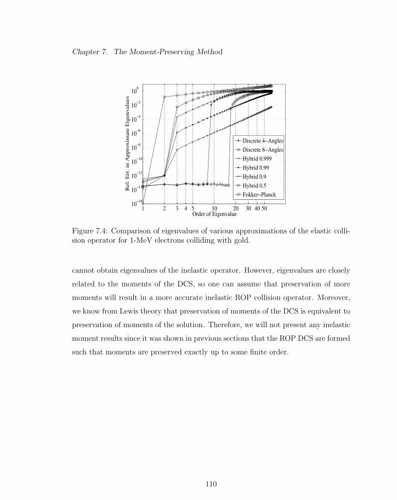
Chapter 7. The Moment-Preserving Method
1 2 3 4 5 10 20 30 40 5010
−16
10−14
10−12
10−10
10−8
10−6
10−4
10−2
100
Order of Eigenvalue
Rel.
Err
. in
Ap
pro
xim
ate
Eig
en
valu
es
Discrete 4−Angles
Discrete 8−Angles
Hybrid 0.999
Hybrid 0.99
Hybrid 0.9
Hybrid 0.5
Fokker−Planck
Figure 7.4: Comparison of eigenvalues of various approximations of the elastic colli-sion operator for 1-MeV electrons colliding with gold.
cannot obtain eigenvalues of the inelastic operator. However, eigenvalues are closely
related to the moments of the DCS, so one can assume that preservation of more
moments will result in a more accurate inelastic ROP collision operator. Moreover,
we know from Lewis theory that preservation of moments of the DCS is equivalent to
preservation of moments of the solution. Therefore, we will not present any inelastic
moment results since it was shown in previous sections that the ROP DCS are formed
such that moments are preserved exactly up to some finite order.
110
Chapter 8
The Geant4 Toolkit
Geant4 is a C++ object-oriented simulation toolkit. The toolkit provides a diverse,
wide-ranging, yet cohesive set of software components which can be employed in a
variety of settings. These range from simple one-off studies of basic phenomena and
geometries to full-scale detector simulations for experiments at the Large Hadron
Collider and other facilities [3]. Geant4 utilizes advanced software engineering tech-
niques to maximize functionality, modularity, extensibility, and openness based on
the Booch methodology. Geant4 is modular and flexible, and the implementation of
the physics is transparent and open to the user such that the user can understand
and customize, or extend, the various classes available in the toolkit. The key do-
mains of Monte Carlo simulation that subsequently led to class categories within the
framework of the Geant4 toolkit include:
• geometry and materials,
• interaction physics,
• tracking management,
• digitization and hit management,
111
Chapter 8. The Geant4 Toolkit
• event and track management,
• visualization and visualization framework,
• user interface.
The following sections discuss how users interact with the toolkit, whether as a
typical user building applications against the toolkit or as an advanced user inter-
ested in toolkit development. The implementation of the Moment-Preserving method
within Geant4 toolkit is detailed including a discussion of the physics classes, the
cross-section construction classes, and the data libraries along with the Geant4 data
processing classes that were utilized.
8.1 Developing with the Geant4 toolkit: Applica-
tion Developers and Toolkit Developers
There are two types of Geant4 developers or users: those that develop simulation
applications for research purposes requiring the development of the mandatory user
classes specific to the users needs and the building of said application against the
toolkit; and those that develop the toolkit itself (toolkit developers are typically
application developers as well). These two types of developers interact with the
toolkit differently.
Application developers do not necessarily need to know the details and the com-
plexities of the entire toolkit. Application developers are typically interested in
solving some specific radiation transport problem for which they have a varying
knowledge of the geometry and materials, the source characteristics (that is, energy,
angular, and spatial dependence), and the necessary physics models. Geant4 pro-
vides the abstract interface for eight user classes, but the concrete implementation,
112
Chapter 8. The Geant4 Toolkit
instantiation and registration of these classes are mandatory for only three of the
eight classes. In other words, Geant4 application developers are required to create a
user specific implementation of the methods specified by the mandatory classes.
These three mandatory classes are G4VUserDetectorConstruction,
G4VUserPhysicsList, and G4VUserPrimaryGeneratorAction, and describe the ge-
ometry and materials, the physics models to be used, and the particle source, respec-
tively. These classes in addition to a main are all that application developers are re-
quired to implement. However, additional user classes are available that can be used
to complete a wide variety of tasks including setting problem parameters, extracting
information, modifying the state of the particle, printing results, and so on. These
user classes include G4UserRunAction, G4UserEventAction, G4UserStackingAction,
G4UserTrackingAction, and G4UserSteppingAction and are all associated with a
“unit of simulation.” That is, the Run, Event, Stack, Track, and Step. The Run is
the largest unit of simulation and is a sequence of Events. An Event includes a source
particle and all of the secondary particles produced by the source particle which are
all classified as Tracks. A Track contains all of the information about a particle from
its birth to its death (primary or secondary). The Stack manages the Tracks and can
be used to prioritize or kill Tracks. The smallest unit of simulation where physics
processes are applied is the Step. With the eight user classes, application developers
can accomplish a great deal by only implementing any number of the optional user
classes. However, possibilities for ambitious Geant4 users are seemingly limitless
with sufficient time and knowledge of the toolkit.
On the other hand, toolkit developers are typically interested in adding classes
relevant to any of the aforementioned class categories to enhance the toolkit. This
does not necessarily require any of the development that was just discussed; however,
toolkit developers are typically application developers as well. In efforts to implement
the Moment-Preserving method, both types of development were undertaken. The
113

Chapter 8. The Geant4 Toolkit
various aspects of the Moment-Preserving method development are discussed in the
following section.
8.2 The Moment-Preserving Method Classes
Reduced order physics DCS models are central to the Moment-Preserving method
and therefore, the majority of the development effort is in generating, storing, and
accessing the ROP DCSs. Geant4 considers all physical interactions as processes,
requiring implementation of the G4VEmProcess class, and the details of each pro-
cess is captured by the model.This is accomplished through implementation of the
G4VEmModel class, which is the primary source of development for the Moment-
Preserving method (assuming the ROP DCS are available in the form of a DCS
data library). The reason that the majority of the development occurs at the level
of implementing the G4VEmModel class is because this is where the ROP DCS are
stored by means of reading-in the data and storing in Geant4 data classes, and this
is where the ROP DCSs are accessed when looking-up the total cross-section and
sampling the DCS.
The other major component of development was creation of the ROP DCS con-
struction classes. These were initially developed and interpreted as stand-alone DCS
objects, in that upon construction of the ROP model class the ROP DCS is con-
structed for every material using the ROP DCS construction classes. This required
that the ROP DCSs were constructed during runtime, which can be relatively CPU
intensive (at most one minute). Further into the development of this method, with a
better understanding of the toolkit, the ROP DCS construction classes were used to
create a library of ROP DCS models making the ROP model classes more compact
and easy to integrate into the toolkit.
The remaining sections provide detail on the associated physics process and model
114

Chapter 8. The Geant4 Toolkit
classes, the cross-section construction classes, and the cross-section library and data
processing tools. In addition, coding examples are provided when possible.
8.2.1 Physics processes
Physics processes for discrete and hybrid DCSs were implemented and include:
• G4DiscreteElasticProcess
• G4HybridSoftElasticProcess
• G4HybridHardElasticProcess
• G4DiscreteInelasticProcess
• G4HybridSoftInelasticProcess
• G4HybridHardInelasticProcess
The physics process is relatively simple because use is made of many of the virtual
functions in G4VEmProcess. For example, G4VEmProcess contains a function for
calling the physics model at the end of a step to sample a collision outcome. A user
can override a virtual function, but only if it is necessary. Therefore, code duplication
is reduced (this is a C++ concept and not specific to Geant4) and the resulting pro-
cess class is very simple. The only functions that required implementation include a
function that initializes the process class (this consists of constructing the associated
physics model and setting a few data members) and a function that determines the
applicable particles.
8.2.2 Physics models
Physics models for discrete and hybrid DCSs were implemented and include:
115
Chapter 8. The Geant4 Toolkit
• G4DiscreteElasticModel
• G4HybridSoftElasticModel
• G4HybridHardElasticModel
• G4DiscreteInelasticModel
• G4HybridSoftInelasticModel
• G4HybridHardInelasticModel
Three important functions are included in the physics model class: an initial-
ization function where the cross-section data is constructed or read in; a function
for obtaining the total cross-section; and a function for sampling the DCS. In de-
veloping the Moment-Preserving method, there were two versions of the associated
physics classes. The early version was designed to be included locally. That is,
in application development the source files specific to the application are stored in
some user working directory. Here, the user develops the mandatory classes and any
additional classes required. It is possible to bring in new physics locally by stor-
ing the classes in this working directory. This approach was used during the early
testing phases and the ROP cross-sections were constructed at runtime. For exam-
ple, in the following lines of code, the crossSection vector is populated with pointers
to GBFPAngularDeflection objects (see section 8.2.3 for detail on the GBFPAngu-
larDeflection cross-section class ). Each object corresponds to a different element
from which the problem materials are composed, so the crossSection vector will have
a length equivalent to the number of elements required by the problem. The draw-
back of this approach is that the GBFPAngularDeflection objects are constructed at
runtime and this adds to the total time for the run. In addition, the Geant4 data
classes make it very straightforward to access data for an element with atomic num-
ber Z. Here, additional functionality must be added to access the correct position
116
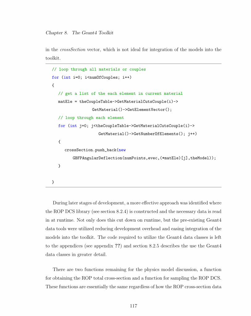
Chapter 8. The Geant4 Toolkit
in the crossSection vector, which is not ideal for integration of the models into the
toolkit.
// loop through all materials or couples
for (int i=0; i<numOfCouples; i++)
// get a list of the each element in current material
matEle = theCoupleTable->GetMaterialCutsCouple(i)->
GetMaterial()->GetElementVector();
// loop through each element
for (int j=0; j<theCoupleTable->GetMaterialCutsCouple(i)->
GetMaterial()->GetNumberOfElements(); j++)
crossSection.push_back(new
GBFPAngularDeflection(numPoints,evec,(*matEle)[j],theModel));
During later stages of development, a more effective approach was identified where
the ROP DCS library (see section 8.2.4) is constructed and the necessary data is read
in at runtime. Not only does this cut down on runtime, but the pre-existing Geant4
data tools were utilized reducing development overhead and easing integration of the
models into the toolkit. The code required to utilize the Geant4 data classes is left
to the appendices (see appendix ??) and section 8.2.5 describes the use the Geant4
data classes in greater detail.
There are two functions remaining for the physics model discussion, a function
for obtaining the ROP total cross-section and a function for sampling the ROP DCS.
These functions are essentially the same regardless of how the ROP cross-section data
117
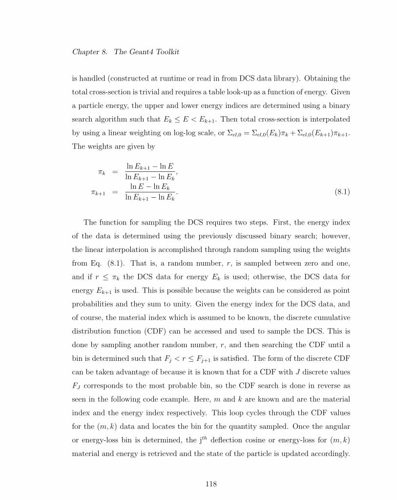
Chapter 8. The Geant4 Toolkit
is handled (constructed at runtime or read in from DCS data library). Obtaining the
total cross-section is trivial and requires a table look-up as a function of energy. Given
a particle energy, the upper and lower energy indices are determined using a binary
search algorithm such that Ek ≤ E < Ek+1. Then total cross-section is interpolated
by using a linear weighting on log-log scale, or Σel,0 = Σel,0(Ek)πk + Σel,0(Ek+1)πk+1.
The weights are given by
πk =lnEk+1 − lnE
lnEk+1 − lnEk,
πk+1 =lnE − lnEk
lnEk+1 − lnEk. (8.1)
The function for sampling the DCS requires two steps. First, the energy index
of the data is determined using the previously discussed binary search; however,
the linear interpolation is accomplished through random sampling using the weights
from Eq. (8.1). That is, a random number, r, is sampled between zero and one,
and if r ≤ πk the DCS data for energy Ek is used; otherwise, the DCS data for
energy Ek+1 is used. This is possible because the weights can be considered as point
probabilities and they sum to unity. Given the energy index for the DCS data, and
of course, the material index which is assumed to be known, the discrete cumulative
distribution function (CDF) can be accessed and used to sample the DCS. This is
done by sampling another random number, r, and then searching the CDF until a
bin is determined such that Fj < r ≤ Fj+1 is satisfied. The form of the discrete CDF
can be taken advantage of because it is known that for a CDF with J discrete values
FJ corresponds to the most probable bin, so the CDF search is done in reverse as
seen in the following code example. Here, m and k are known and are the material
index and the energy index respectively. This loop cycles through the CDF values
for the (m, k) data and locates the bin for the quantity sampled. Once the angular
or energy-loss bin is determined, the jth deflection cosine or energy-loss for (m, k)
material and energy is retrieved and the state of the particle is updated accordingly.
118
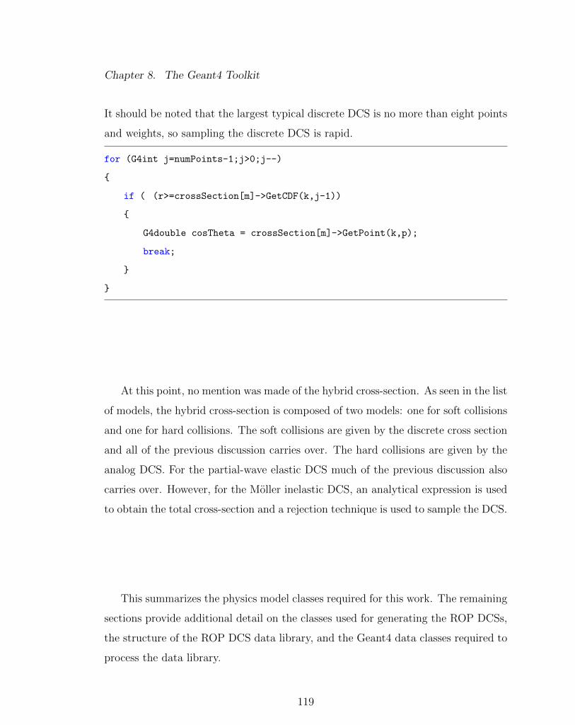
Chapter 8. The Geant4 Toolkit
It should be noted that the largest typical discrete DCS is no more than eight points
and weights, so sampling the discrete DCS is rapid.
for (G4int j=numPoints-1;j>0;j--)
if ( (r>=crossSection[m]->GetCDF(k,j-1))
G4double cosTheta = crossSection[m]->GetPoint(k,p);
break;
At this point, no mention was made of the hybrid cross-section. As seen in the list
of models, the hybrid cross-section is composed of two models: one for soft collisions
and one for hard collisions. The soft collisions are given by the discrete cross section
and all of the previous discussion carries over. The hard collisions are given by the
analog DCS. For the partial-wave elastic DCS much of the previous discussion also
carries over. However, for the Moller inelastic DCS, an analytical expression is used
to obtain the total cross-section and a rejection technique is used to sample the DCS.
This summarizes the physics model classes required for this work. The remaining
sections provide additional detail on the classes used for generating the ROP DCSs,
the structure of the ROP DCS data library, and the Geant4 data classes required to
process the data library.
119

Chapter 8. The Geant4 Toolkit
8.2.3 Cross-section construction
All ROP DCS classes inherit from the GBFPCrossSection1 base class. The
GBFPCrossSection base class contains data members and functions required to gen-
erate an ROP DCS. The data members include vectors for storing ROP DCS points
and weights, CDFs, and total cross-sections, along with vectors associated with the
quadrature functions like coefficients of Legendre polynomials and Gauss-Legendre
quadrature points and weights. The critical functions include the function for the
modified Chebyshev algorithm and the function for obtaining Radau quadrature
which includes a matrix eigenvalue solver (see Chapter 7 for details). The ROP
DCSs are generated when constructing either a GBFPAngularDeflection or a
GBFPMollerEnergyLoss object. The GBFPAngularDeflection or
GBFPMollerEnergyLoss classes have data members and functions specific to elastic
and inelastic DCSs respectively. Here, an outline of the algorithm for generating a
discrete DCS is provided with some coding examples.
When a GBFPAngularDeflection object is created,
GBFPAngularDeflection* crossSection
= new GBFPAngularDeflection(numPoints,evec,(*matEle)[j],theModel);
data members are initialized. For example, the vectors points, CDF, and Sigmat are
sized appropriately and set to zero.
points.resize(energyGrid.size()); CDF.resize(energyGrid.size());
Sigmat.resize(energyGrid.size()); int N = numberOfPoints;
for (int i = 0; i < energyGrid.size(); i++)
points[i].resize(N,0.0); CDF[i].resize(N,0.0);
1The significance of GBFP is from the previous naming of the method; that is, the GeneralizedBoltzmann Fokker-Planck method [60].
120

Chapter 8. The Geant4 Toolkit
In addition, vectors for the coefficients for Legendre polynomials are populated
and local or temporary vectors for storing the coefficients of the polynomials orthog-
onal with respect to the analog DCS are initialized along with vectors for temporarily
storing points and weights.
vector<double> alpha = GetALeg(); // coefficient of Legendre polynomials
vector<double> beta = GetBLeg(); // coefficient of Legendre polynomials
// Temp vectors for coefficient of special polynomials (aa,bb)
// and points and weights (x,w)
vector<double> aa(N,0.0), bb(N,0.0), x(N,0.0), w(N,0.0);
Once the necessary data members are initialized, a loop over all energies is executed,
where the ROP DCSs for the current material are generated for each energy. Below,
the associated code is provided for generating a discrete elastic DCS based on the
screened Rutherford analog DCS. For a given energy, the parameters defining the
screened Rutherford DCS are determined. That is, the screening parameter and the
material constant (eta and CC). Now that the analog DCS is completely described,
moments of the DCS are generated using an adaptive quadrature technique. The
modified Chebyshev algorithm (MCA) requires monic moments, so the moments are
then renormalized. These moments, along with the coefficients of monic Legendre
polynomials (that is, Ml, alpha, and beta) are passed to the MCA. The MCA then
returns the coefficients of polynomials that are orthogonal with respect the screened
Rutherford DCS. These coefficients (aa and bb) are passed to the Radau function
where a tridiagonal matrix is setup and the discrete points and weights are deter-
mined from this matrix (that is, the Jacobi matrix). The points and weights returned
by the Radau function, must be regularized. The Regularize function removes the
N + 1 point and weight, and then multiplies the remaining points and weights by
the total cross section, Ml[0] because the weights passed to Regularize sum to unity.
121

Chapter 8. The Geant4 Toolkit
Prior to storing the DCS data, testing is completed to ensure meaningful data. The
discrete points are stored as the weights are summed. The sum of the weights are
then stored in the total cross-section vector and a CDF is generated and stored as
well. All of the temporary vectors are cleared and reset to zero. The process then
continues for the next energy. The cross-section generation classes are provided in
appendix ??.
for (int i=0; i<E.size(); i++)
G4double eta =
model->CalculateScreeningParameter(E[i], 0.51099891, ele->GetZ());
G4double CC =
model->CalculateMaterialConstant(E[i], 0.51099891, ele->GetZ());
SetAngularDeflectionMomentsWithAdaptiveQuadrature(E[i],CC,eta,Ml);
Monic(Ml);
orthog(Ml,alpha,beta,aa,bb);
Radau(aa,bb,x,w);
Regularize(x,w,Ml[0]);
// Testing of points and weights removed for compactness
// in coding example
sum = 0.;
for (int j=0; j<x.size(); j++)
SetPoint(i,j,x[j]); sum += w[j]; SetCDF(i,j,sum);
SetSigt(i,sum);
for (int j=0; j<x.size(); j++)SetCDF(i,j,GetCDF(i,j)/sum);
//normalizing CDF
aa.clear(), bb.clear(), x.clear(), w.clear(), Ml.clear();
aa.resize(N,0.0), bb.resize(N,0.0), x.resize(N,0.0), w.resize(N,0.0),
Ml.resize(2*N,0.0);
122
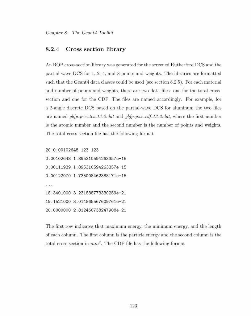
Chapter 8. The Geant4 Toolkit
8.2.4 Cross section library
An ROP cross-section library was generated for the screened Rutherford DCS and the
partial-wave DCS for 1, 2, 4, and 8 points and weights. The libraries are formatted
such that the Geant4 data classes could be used (see section 8.2.5). For each material
and number of points and weights, there are two data files: one for the total cross-
section and one for the CDF. The files are named accordingly. For example, for
a 2-angle discrete DCS based on the partial-wave DCS for aluminum the two files
are named gbfp pwe tcs 13 2.dat and gbfp pwe cdf 13 2.dat, where the first number
is the atomic number and the second number is the number of points and weights.
The total cross-section file has the following format
20 0.00102648 123 123
0.00102648 1.895310594263357e-15
0.00111939 1.895310594263357e-15
0.00122070 1.735008462388171e-15
...
18.3401000 3.231888773330259e-21
19.1521000 3.014865567609761e-21
20.0000000 2.812460738247908e-21
The first row indicates that maximum energy, the minimum energy, and the length
of each column. The first column is the particle energy and the second column is the
total cross section in mm2. The CDF file has the following format
123
Chapter 8. The Geant4 Toolkit
0.1253630590705352 -0.5474023266341548
1.0000000000000000 0.7102211565388719
0.1253630590705352 -0.5474023266341548
1.0000000000000000 0.7102211565388719
0.1176158475868398 -0.5376566009643416
1.0000000000000000 0.7163622043775827
...
0.0013006768714632 -0.0091294921937126
1.0000000000000000 0.9732752885064547
0.0012783923557266 -0.0076636446407933
1.0000000000000000 0.9735167107563724
0.0012560788028267 -0.0060866632871608
1.0000000000000000 0.9737602097136864
The first column is the value of the CDF for some discrete angle and because this is
a 2-angle data file, every two values corresponds to one energy. The second column
is the discrete angle associated with the CDF.
The next section discusses the Geant4 data classes required and the how the data
files are processed.
8.2.5 Data processing
There are two primary Geant4 data classes utilized in processing and storing the ROP
DCS data: G4ElementData and G4PhysicsVector. G4ElementData is a very powerful
class that stores data for a particular element and then only requires the atomic
number to retrieve the data. Upon construction, the G4ElementData object requires
the atomic number and the data in the form of a pointer to a G4PhysicsVector object,
so the G4ElementData class is really a container of G4PhysicsVector objects. The
124

Chapter 8. The Geant4 Toolkit
data is actually stored in the G4PhysicsVector object, which is also a very powerful
class because as long as the data is properly formatted, one must simply pass the
G4PhysicsVector object a stream of the data.
As an example, the process of reading total cross-section data is provided, where
tcs is a pointer to a G4ElementData object. First, in the initialize function of the
G4DiscreteElasticModel, the materials and their constituents are processed. The
atomic number of the current element is determined and a check is performed to
determine if the data already exist. If it does not exist, ReadData is called with the
material Z and the path to the data.
for(G4int i=0; i<numOfCouples; ++i)
const G4Material* material =
theCoupleTable->GetMaterialCutsCouple(i)->GetMaterial();
const G4ElementVector* theElementVector = material->GetElementVector();
G4int nelm = material->GetNumberOfElements();
// loop through all elements
// if data for element does not exist process it
for (G4int j=0; j<nelm; ++j)
G4int Z = (G4int)(*theElementVector)[j]->GetZ();
else if(Z > maxZ) Z = maxZ;
if(!tcs->GetElementData(Z)) ReadData(Z, path);
The following code provides an example of what occurs inside ReadData specifically
for processing the total cross-section data. First, a stream is opened for the total
cross-section data determined by the path to the data file. A temporary pointer
to a G4PhysicsVector object is constructed. Then the Retrieve function is used to
read in the data for the current stream. Once the data is read in, the pointer to the
G4PhysicsVector object containing the data is passed to the G4ElementData object,
125
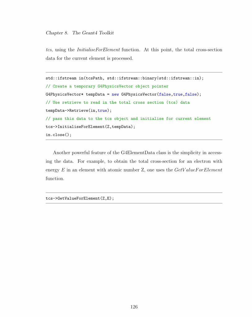
Chapter 8. The Geant4 Toolkit
tcs, using the InitialiseForElement function. At this point, the total cross-section
data for the current element is processed.
std::ifstream in(tcsPath, std::ifstream::binary|std::ifstream::in);
// Create a temporary G4PhysicsVector object pointer
G4PhysicsVector* tempData = new G4PhysicsVector(false,true,false);
// Use retrieve to read in the total cross section (tcs) data
tempData->Retrieve(in,true);
// pass this data to the tcs object and initialise for current element
tcs->InitialiseForElement(Z,tempData);
in.close();
Another powerful feature of the G4ElementData class is the simplicity in access-
ing the data. For example, to obtain the total cross-section for an electron with
energy E in an element with atomic number Z, one uses the GetV alueForElement
function.
tcs->GetValueForElement(Z,E);
126

Chapter 9
Results
In this chapter, a wide array of results that capture the key features of the Moment-
Preserving (MP) method are presented. In particular, the key features of this method
demonstrated are:
• systematic accuracy,
• efficient,
• mathematically robust,
• versatile,
• simple.
The results section begins by demonstrating the first feature of the MP method
through calculation of highly differential quantities like angular distributions and
energy spectra. In these calculations, the MP method is tested under the strictest
possible conditions (that is, high-energy mono-energetic pencil beams normally in-
cident on thin slabs). Under these conditions, analog or single-scatter models are
127

Chapter 9. Results
typically required. However, it is shown that both transmitted and reflected angular
distributions and energy-loss spectra can be resolved through use of the hybrid DCS.
Though the emphasis of this section is the demonstration of the systematic nature of
the MP method, efficiency gains of at least five times analog efficiencies were demon-
strated while maintaining analog level accuracy in very thin slabs. Under these
extreme conditions where the hybrid model is successful, the discrete model tends to
result in artifacts. However, it is possible to utilize the discrete model in thicker slabs
where the benefit of efficiency gains is significantly improved. Following the angular
distribution and energy spectrum results, longitudinal and lateral distributions are
presented where the first two features of the method are again demonstrated on this
different, but important quantity.
Given a clear understanding of the systematic feature of this method, results
for less extreme problem conditions are presented to show that for more practical
applications the MP method is not just accurate, but also very efficient. That is, we
show that for 1-D and 2-D dose calculations the MP method achieves analog level
accuracy while improving efficiency up to three orders of magnitude over analog
efficiencies. We show that this is true for low-Z and high-Z materials, for molecules
like water or bone, and multi-region problems. Furthermore, it is shown that material
interfaces in multi-region problems do not introduce additional error at interfaces as
does the condensed history method. This is because the MP method is a transport-
based approximation and the benefit of this type of approach is that no additional
algorithm is required to handle material interfaces.
Prior to this work, no effort had been made to validate the MP method through
comparison with experimental benchmarks. Therefore, several results are presented
in efforts to begin this validation process. Specifically, results from the MP method
are compared to the experimentally determined energy deposition profiles (that is,
the Lockwood data [81]). Similar calculations are made with the Geant4 default elec-
128

Chapter 9. Results
tromagnetic physics option 3, so that accuracy and efficiencies for the MP method
can be compared to the Geant4 physics. In addition, we compare charge deposition
results generated using MP method with experimentally determined charge deposi-
tions (that is, the Tabata data [82]). A key concept to point out in comparing with
experimental results is that if an analog model exists that is in acceptable agreement
with an experimental benchmark and moments of this analog model are readily
available, one can generate reduced order physics DCSs based on the aforementioned
analog model and show similar levels of agreement while significantly improving ef-
ficient. In this sense, the versatility and simplicity of the method is demonstrated.
That is, to improve agreement through use of a different analog model algorithmic
changes are not required; one must simply obtain moments of some preferable analog
model, generate an ROP DCS library for this analog model, and run the calculation.
Finally, for completeness the MP method is applied to a space weather application
to show that this method is not just effective for theoretical calculations. In particu-
lar, the total response function is generated for the CEASE detector telescope using
an analog model, a discrete model, and the default Geant4 electromagnetic physics
with option 3.
In all comparisons, the analog benchmark is obtained by using an analog elastic
DCS and an analog inelastic DCS (with exception of the validation section). The
analog benchmark is numerical rather than experimental, so to some degree it is ide-
alized. This type of benchmarking is required to illustrate how accuracy is achieved
through preservation of the analog DCS moments. In the following sections, accuracy
and efficiency is measured with respect to the analog benchmark.
129

Chapter 9. Results
9.1 Angular Distributions and Energy Spectra
In this section, the accuracy of the MP method is tested under conditions that are
often times impractical to simulate without the use of an analog model. That is, the
transport of a mono-energetic pencil beam of electrons with energies above several
hundred keV in thin slabs. Of particular interest is the calculation of reflected and
transmitted angular distributions and energy spectra in slabs with varying thick-
nesses down to 100 analog elastic mfps (∼ 1 to 100 µm). It is shown that under
these conditions the MP method is effective at resolving angular distributions and
energy spectra through the use of suitable reduced order physics (ROP) DCSs. Un-
der these extreme conditions, a hybrid DCS is, in most cases, required to resolve
these distributions. While it is possible to resolve highly peaked distributions with
analog level accuracy using the MP method, this is typically accompanied by losses
in efficiency. Nonetheless, the ability to systematically control accuracy such that
one can predict angular distributions and energy spectra for highly-peaked scattering
in thin slabs is a strong feature of this method.
While it is true that one cannot expect to realize significant efficiency gains with
analog level accuracy under the aforementioned conditions, in more realistic settings
(that is, thicker regions) it is possible to relax the ROP models such that both analog
level accuracy and significant efficiency gains are achieved. Relaxation of the ROP
models is possible in thicker slabs because the initial pencil beam experiences more
spreading in space, angle, and energy in thicker slabs. This is simply an effect of
the number of collisions sustained by an electron while traversing a medium. In
thicker slabs, electrons suffer more collisions; thus, causing additional spreading of
the initial state of the beam. With additional spreading of the beam, less information
in the form of analog DCS moments is required to resolve angular distributions and
energy spectra. Therefore, the ROP DCS can be relaxed or models preserving fewer
moments can be utilized.
130

Chapter 9. Results
In the following two sections, the impact of the size of the slab on the accuracy
of the MP method is demonstrated. Both discrete and hybrid models are tested for
angular distribution and energy spectrum calculations in low-Z and high-Z slabs with
varying thicknesses. The thickness of the slab is measured with respect to the analog
elastic mfp corresponding to the source particle energy and the target material.
Results for slabs with thicknesses of 100, 300, 1000, and 3000 analog elastic mfps are
presented (in the remaining discussion mfp implies analog elastic mfp). In Fig. 9.1,
problem setup is described.
Figure 9.1: Problem setup for calculation of angular distributions and energy spectra.
9.1.1 Angular distributions
Reflected and transmitted angular distributions are presented below for one-dimensional
slabs composed of aluminum or gold with thicknesses of 100, 300, 1000, and 3000
mfps (that is, L = 100λel, 300λel, 1000λel, 3000λel). The source is positioned at
x = 0 with a direction of ~Ω = (1, 0, 0). A total of 4× 10⁷ source particles are simu-
lated when calculating the angular distributions. The analog benchmark is a solution
to the aforementioned problem using analog Monte Carlo, where elastic scattering is
131

Chapter 9. Results
given by the partial-wave DCS and inelastic scattering is given by the Moller DCS.
Uncertainties associated with these results are within 1% in most bins, such that one
can state conclusively that good agreement exists between the ROP models and the
analog benchmark.
First, the most challenging problem is presented. That is, calculation of transmit-
ted angular distributions for 10000-keV electrons incident on an aluminum or gold
slab 100 mfps thick. In Figs. 9.2a and 9.2b, transmitted angular distributions in
aluminum and gold computed using the discrete and hybrid DCSs are compared to
the analog benchmark. There are a few features to note in Fig. 9.2. The peakedness
of this distribution is extreme and varies about three orders of magnitude over only
10 degrees. This level of peakedness is difficult to resolve with a discrete elastic DCS
and results in the discrete artifacts seen clearly in the Figs. 9.2a and 9.2b. The dif-
ficulty in resolving highly peaked distributions using the discrete DCS results from
the form of the DCS. That is, electrons can only scatter through N discrete angles
determined by the order of the DCS. Therefore, the N discrete angles are favored
in the angular distribution because in thin slabs electrons do not suffer enough col-
lisions such that various combinations of scattering events smooth out the artifacts.
However, through use of the hybrid model the discrete artifacts are mitigated and the
only noticeable differences in the hybrid model solution and the analog benchmark
are in the tail where the differences in the solutions are statistically insignificant.
In Fig. 9.2c, the impact of target atomic number is shown, where for increasing Z
the distribution is less-peaked. However, the impact of the atomic number on the
peakedness of the scattering is not significant enough to dramatically improve the
discrete results in thin slabs for 10000-keV electrons.
Even in aluminum slabs with thicknesses of 3000 mfps for 10000-keV electrons,
the discrete DCS results in artifacts as seen in Fig. 9.3a. This is an indication of the
extreme peakedness of the scattering at higher energies and in this regime a hybrid
132

Chapter 9. Results
0 10 20 30 40 50 60 70 80 90
10−6
10−4
10−2
100
102
θ (degrees)
p(L
,θ)
Partial−wave + Moller
Discrete 4−Angles, 4−Energies
Hybrid 1−Angle, cut=0.999, 4−Energies
(a) Aluminum
0 10 20 30 40 50 60 70 80 90
10−6
10−4
10−2
100
102
p(L
,θ)
Partial−wave + Moller
Discrete 4−Angles, 4−Energies
Hybrid 1−Angle, cut=0.999, 4−Energies
(b) Gold
0 10 20 30 40 50 60 70 80 9010
−6
10−4
10−2
100
102
θ (degrees)
p(L
,θ)
Aluminum
Gold
(c) Analog Benchmark
Figure 9.2: Transmitted angular distributions for 10000-keV electrons on 100 mfpthick aluminum (a) and gold (b) slabs calculated using the analog model (solid black),a purely discrete model with 4-angles and 4-energies (solid blue), and a hybrid elasticmodel with a single angle and µ∗ = 0.999 and a discrete inelastic model with 4-energies (dashed red). The analog benchmarks (c) are in black for aluminum andblue for gold.
DCS is required to resolve the transmitted angular distribution unless additional
angles are used. However, it is clear by Figs. 9.3a and 9.3b that in thicker slabs
where particles undergo thousands of collisions that the discrete artifacts are greatly
reduced. Furthermore, the impact of the atomic number is seen in Fig. 9.3b, where
the discrete artifacts are less pronounced in the gold slab because scattering of elec-
trons by high-Z materials is less peaked. Nonetheless, it is always possible to utilize
a hybrid model to resolve angular distributions overwhelmed by discrete artifacts.
133
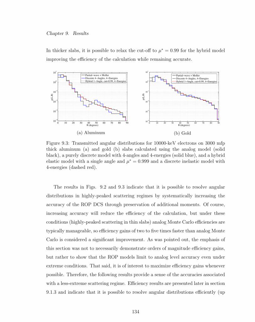
Chapter 9. Results
In thicker slabs, it is possible to relax the cut-off to µ∗ = 0.99 for the hybrid model
improving the efficiency of the calculation while remaining accurate.
0 10 20 30 40 50 60 70 80 9010
−4
10−3
10−2
10−1
100
101
θ (degrees)
p(L
,θ)
Partial−wave + Moller
Discrete 4−Angles, 4−Energies
Hybrid 1−Angle, cut=0.99, 4−Energies
(a) Aluminum
0 10 20 30 40 50 60 70 80 9010
−4
10−3
10−2
10−1
100
101
θ (degrees)
p(L
,θ)
Partial−wave + Moller
Discrete 4−Angles, 4−Energies
Hybrid 1−Angle, cut=0.99, 4−Energies
(b) Gold
Figure 9.3: Transmitted angular distributions for 10000-keV electrons on 3000 mfpthick aluminum (a) and gold (b) slabs calculated using the analog model (solidblack), a purely discrete model with 4-angles and 4-energies (solid blue), and a hybridelastic model with a single angle and µ∗ = 0.999 and a discrete inelastic model with4-energies (dashed red).
The results in Figs. 9.2 and 9.3 indicate that it is possible to resolve angular
distributions in highly-peaked scattering regimes by systematically increasing the
accuracy of the ROP DCS through preservation of additional moments. Of course,
increasing accuracy will reduce the efficiency of the calculation, but under these
conditions (highly-peaked scattering in thin slabs) analog Monte Carlo efficiencies are
typically manageable, so efficiency gains of two to five times faster than analog Monte
Carlo is considered a significant improvement. As was pointed out, the emphasis of
this section was not to necessarily demonstrate orders of magnitude efficiency gains,
but rather to show that the ROP models limit to analog level accuracy even under
extreme conditions. That said, it is of interest to maximize efficiency gains whenever
possible. Therefore, the following results provide a sense of the accuracies associated
with a less-extreme scattering regime. Efficiency results are presented later in section
9.1.3 and indicate that it is possible to resolve angular distributions efficiently (up
134

Chapter 9. Results
to two orders of magnitude more efficient than analog) and accurately; especially, in
less-extreme scattering regimes.
The following figures present transmitted angular distributions in a less-peaked
scattering regime. That is, 1000-keV electrons incident on gold slabs with varying
thicknesses. As noted, the peakedness of the scattering is a function of particle
energy and the target atomic number. With decreased particle energy and increased
atomic number, the peakedness is reduced. Nonetheless, even for 1000-keV electrons
on gold the problem is still extremely anisotropic with respect to neutral particle
scattering. In Fig. 9.4, the impact of slab thickness and in turn, the effectiveness
of the discrete model is demonstrated. In Figs. 9.4a and 9.4b, discrete artifacts are
present for slabs 100 and 300 mfps thick, but the hybrid model is in good agreement
in these cases. However, in Figs. 9.4c and 9.4d, discrete models with at most 4-
angles are sufficient when resolving the transmitted angular distribution. In fact,
in Fig. 9.4d the discrete artifacts resulting from a single-angle discrete model are
almost negligible and though there is not perfect agreement the general behavior of
the transmitted angular distribution is captured.
135
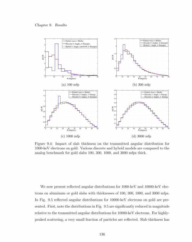
Chapter 9. Results
0 10 20 30 40 50 600
1
2
3
4
5
6
θ (degrees)
p(L
,θ)
Partial−wave + Moller
Discrete 4−Angles, 4−Energies
Hybrid 1−Angle, cute=0.99, 4−Energies
(a) 100 mfp
0 10 20 30 40 50 60 70 80 900
0.5
1
1.5
2
2.5
θ (degrees)
p(L
,θ)
Partial−wave + Moller
Discrete 4−Angles, 4−Energies
Hybrid 1−Angle, 4−Energies
(b) 300 mfp
0 10 20 30 40 50 60 70 80 900
0.2
0.4
0.6
0.8
1
1.2
1.4
θ (degrees)
p(L
,θ)
Partial−wave + Moller
Discrete 2−Angles, 1−Energy
Discrete 4−Angles, 4−Energies
(c) 1000 mfp
0 10 20 30 40 50 60 70 80 900
0.1
0.2
0.3
0.4
0.5
0.6
0.7
0.8
0.9
θ (degrees)
p(L
,θ)
Partial−wave + Moller
Discrete 1−Angle, 1−Energy
Discrete 2−Angles, 1−Energy
(d) 3000 mfp
Figure 9.4: Impact of slab thickness on the transmitted angular distribution for1000-keV electrons on gold. Various discrete and hybrid models are compared to theanalog benchmark for gold slabs 100, 300, 1000, and 3000 mfps thick.
We now present reflected angular distributions for 1000-keV and 10000-keV elec-
trons on aluminum or gold slabs with thicknesses of 100, 300, 1000, and 3000 mfps.
In Fig. 9.5 reflected angular distributions for 10000-keV electrons on gold are pre-
sented. First, note the distributions in Fig. 9.5 are significantly reduced in magnitude
relative to the transmitted angular distributions for 10000-keV electrons. For highly-
peaked scattering, a very small fraction of particles are reflected. Slab thickness has
136
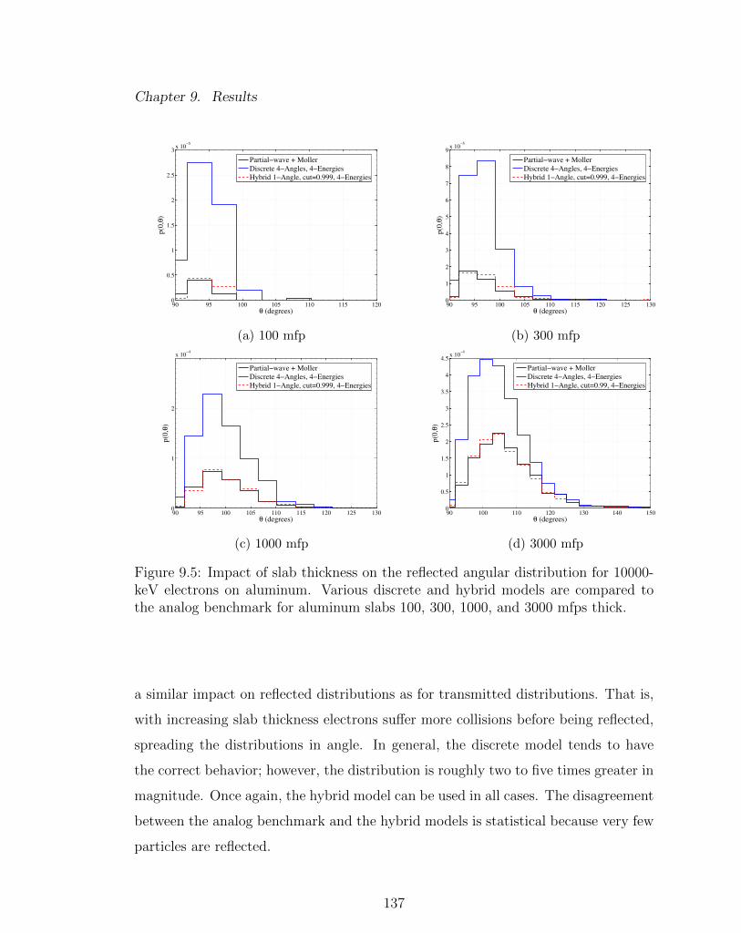
Chapter 9. Results
90 95 100 105 110 115 1200
0.5
1
1.5
2
2.5
3x 10
−5
θ (degrees)
p(0
,θ)
Partial−wave + Moller
Discrete 4−Angles, 4−Energies
Hybrid 1−Angle, cut=0.999, 4−Energies
(a) 100 mfp
90 95 100 105 110 115 120 125 1300
1
2
3
4
5
6
7
8
9x 10
−5
θ (degrees)
p(0
,θ)
Partial−wave + Moller
Discrete 4−Angles, 4−Energies
Hybrid 1−Angle, cut=0.999, 4−Energies
(b) 300 mfp
90 95 100 105 110 115 120 125 1300
1
2
x 10−4
θ (degrees)
p(0
,θ)
Partial−wave + Moller
Discrete 4−Angles, 4−Energies
Hybrid 1−Angle, cut=0.999, 4−Energies
(c) 1000 mfp
90 100 110 120 130 140 1500
0.5
1
1.5
2
2.5
3
3.5
4
4.5x 10
−4
θ (degrees)
p(0
,θ)
Partial−wave + Moller
Discrete 4−Angles, 4−Energies
Hybrid 1−Angle, cut=0.99, 4−Energies
(d) 3000 mfp
Figure 9.5: Impact of slab thickness on the reflected angular distribution for 10000-keV electrons on aluminum. Various discrete and hybrid models are compared tothe analog benchmark for aluminum slabs 100, 300, 1000, and 3000 mfps thick.
a similar impact on reflected distributions as for transmitted distributions. That is,
with increasing slab thickness electrons suffer more collisions before being reflected,
spreading the distributions in angle. In general, the discrete model tends to have
the correct behavior; however, the distribution is roughly two to five times greater in
magnitude. Once again, the hybrid model can be used in all cases. The disagreement
between the analog benchmark and the hybrid models is statistical because very few
particles are reflected.
137

Chapter 9. Results
In Fig. 9.6 angular distributions for 1000-keV electrons incident on gold slabs
with thicknesses of 100, 300, 1000, and 3000 mfps are presented. For lower energies
in high-Z materials the scattering is less-peaked and the ROP model can be relaxed
under these conditions. Specifically, reflected angular distributions generated using
the discrete model are not overwhelmed by artifacts as seen in Fig. 9.6. For slabs
of sufficient thickness, a hybrid model is not required and the more efficient discrete
model can be utilized. For slabs that are 3000 mfps thick (Fig. 9.6d), a single-angle,
single-energy discrete model provides noteworthy agreement.
90 100 110 120 130 140 150 160 1700
1
2
3
4
5
6
7x 10
−3
θ (degrees)
p(0
,θ)
Partial−wave + Moller
Discrete 4−Angles, 4−Energies
Hybrid 1−Angle, cut=0.99, 4−Energies
(a) 100 mfp
90 100 110 120 130 140 150 160 170 1800
0.005
0.01
0.015
0.02
0.025
0.03
0.035
θ (degrees)
p(0
,θ)
Partial−wave + Moller
Discrete 4−Angles, 4−Energies
Hybrid 1−Angle, cut=0.99, 4−Energies
(b) 300 mfp
90 100 110 120 130 140 150 160 170 1800
0.05
0.1
0.15
0.2
0.25
θ (degrees)
p(0
,θ)
Partial−wave + Moller
Discrete 2−Angles, 1−Energy
Discrete 4−Angles, 4−Energies
(c) 1000 mfp
90 100 110 120 130 140 150 160 170 1800
0.1
0.2
0.3
0.4
0.5
0.6
θ (degrees)
p(0
,θ)
Partial−wave + Moller
Discrete 1−Angle, 1−Energy
Discrete 2−Angles, 1−Energy
(d) 3000 mfp
Figure 9.6: Impact of slab thickness on the reflected angular distribution for 1000-keV electrons on gold. Various discrete and hybrid models are compared to theanalog benchmark for gold slabs 100, 300, 1000, and 3000 mfps thick.
138

Chapter 9. Results
9.1.2 Energy spectra
Next, reflected and transmitted energy spectra are examined. The simulation charac-
teristics, including slab thickness, material types, and the number of source particles,
are the same as described in the previous section. Discrete inelastic DCS models are
not presented because a sufficient number of inelastic collisions do not occur in thin
slabs overwhelming the spectra with discrete artifacts. Therefore, the focus is on
two different hybrid inelastic DCS models. The hybrid models include DCSs with
Q∗ = 10-keV and one or two discrete energies. In each of the following results, elas-
tic scattering is modeled by a discrete four-angle DCS. Again, the most challenging
problem, 10000-keV electrons on aluminum slabs, is considered first. In Fig. 9.8,
transmitted energy-loss spectra are presented for aluminum slabs with thicknesses
of 100, 300, 1000, and 3000 mfps. As seen in Fig. 9.7, it is possible to resolve the
transmitted energy-loss spectra with a sufficiently accurate hybrid inelastic model.
For 10000-keV electrons on aluminum, a two-energy hybrid model is required. How-
ever, for 1000-keV electrons on gold, it is possible to relax the inelastic model to a
single energy with the same cut-off. In Fig. 9.8, results for 1000-keV electrons on
gold are presented. Under these conditions, inelastic scattering is also less-peaked
and the hybrid model can be relaxed. However, a discrete representation is still not
sufficient.
139

Chapter 9. Results
0 1 2 3 4 5 6 710
−8
10−6
10−4
10−2
100
102
E0−E (MeV)
p(L
,E0−
E)
(MeV
−1)
Partial−wave + Moller
Discrete 4−Angles, Hybrid 2−Energies, cut=10−keV
(a) 100 mfp
0 1 2 3 4 5 6 7 810
−8
10−6
10−4
10−2
100
102
E0−E (MeV)
p(L
,E0−
E)
(MeV
−1)
Partial−wave + Moller
Discrete 4−Angles, Hybrid 2−Energies, cut=10−keV
(b) 300 mfp
0 1 2 3 4 5 6 7 810
−8
10−6
10−4
10−2
100
102
E0−E (MeV)
p(L
,E0−
E)
(MeV
−1)
Partial−wave + Moller
Discrete 4−Angles, Hybrid 2−Energies, cut=10−keV
(c) 1000 mfp
0 1 2 3 4 5 6 7 8 910
−8
10−6
10−4
10−2
100
102
E0−E (MeV)
p(L
,E0−
E)
(MeV
−1)
Partial−wave + Moller
Discrete 4−Angles, Hybrid 2−Energies, cut=10−keV
(d) 3000 mfp
Figure 9.7: Impact of slab thickness on the transmitted energy-loss spectra for 10000-keV electrons on aluminum slabs 100, 300, 1000, and 3000 mfps thick.
140
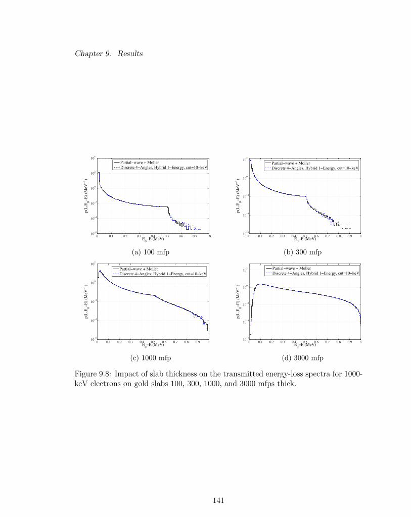
Chapter 9. Results
0 0.1 0.2 0.3 0.4 0.5 0.6 0.7 0.810
−6
10−4
10−2
100
102
104
E0−E (MeV)
p(L
,E0−
E)
(MeV
−1)
Partial−wave + Moller
Discrete 4−Angles, Hybrid 1−Energy, cut=10−keV
(a) 100 mfp
0 0.1 0.2 0.3 0.4 0.5 0.6 0.7 0.8 0.9 110
−6
10−4
10−2
100
102
E0−E (MeV)
p(L
,E0−
E)
(MeV
−1)
Partial−wave + Moller
Discrete 4−Angles, Hybrid 1−Energy, cut=10−keV
(b) 300 mfp
0 0.1 0.2 0.3 0.4 0.5 0.6 0.7 0.8 0.9 110
−6
10−4
10−2
100
102
E0−E (MeV)
p(L
,E0−
E)
(MeV
−1)
Partial−wave + Moller
Discrete 4−Angles, Hybrid 1−Energy, cut=10−keV
(c) 1000 mfp
0 0.1 0.2 0.3 0.4 0.5 0.6 0.7 0.8 0.9 110
−6
10−4
10−2
100
102
E0−E (MeV)
p(L
,E0−
E)
(MeV
−1)
Partial−wave + Moller
Discrete 4−Angles, Hybrid 1−Energy, cut=10−keV
(d) 3000 mfp
Figure 9.8: Impact of slab thickness on the transmitted energy-loss spectra for 1000-keV electrons on gold slabs 100, 300, 1000, and 3000 mfps thick.
141

Chapter 9. Results
Reflected energy-loss spectra for 10000-keV and 1000-keV electrons on gold are
presented next. Reflected energy-loss spectra for 10000-keV electrons on aluminum
are not presented because the reflected electrons experience almost no inelastic colli-
sions. This is true even for gold as seen in Figs. 9.9a and 9.9b for slabs that are 100
and 300 analog mfps thick, where the distributions are nearly singular about zero
energy-loss. That said, the hybrid model also predicts this nearly singular behav-
ior. For thicker slabs, 1000 and 3000 analog mfps, the reflected energy-loss spectra
spreads out more. Here, the hybrid model is in good agreement in the statistically
significant regions of the spectra (that is, the peaked region of the spectra).
0 0.5 1 1.5 2 2.510
−7
10−6
10−5
10−4
10−3
E0−E (MeV)
p(0
,E0−
E)
(MeV
−1)
Partial−wave + Moller
Discrete 4−Angles, Hybrid 2−Energies, cut=10−keV
(a) 100 mfp
0 0.5 1 1.5 2 2.5 3 3.5 410
−7
10−6
10−5
10−4
10−3
E0−E (MeV)
p(0
,E0−
E)
(MeV
−1)
Partial−wave + Moller
Discrete 4−Angles, Hybrid 2−Energies, cut=10−keV
(b) 300 mfp
0 1 2 3 4 5 610
−7
10−6
10−5
10−4
10−3
10−2
E0−E (MeV)
p(0
,E0−
E)
(MeV
−1)
Partial−wave + Moller
Discrete 4−Angles, Hybrid 2−Energies, cut=10−keV
(c) 1000 mfp
0 1 2 3 4 5 610
−7
10−6
10−5
10−4
10−3
10−2
E0−E (MeV)
p(0
,E0−
E)
(MeV
−1)
Partial−wave + Moller
Discrete 4−Angles, Hybrid 2−Energies, cut=10−keV
(d) 3000 mfp
Figure 9.9: Impact of slab thickness on the reflected energy-loss spectra for 10000-keV electrons on gold slabs 100, 300, 1000, and 3000 mfps thick.
142

Chapter 9. Results
In Fig. 9.10, reflected energy-loss spectra are presented for 1000-keV electrons on
gold. Once again, in this less-peaked regime the spectra are not nearly as singular
and a relaxed, single-energy hybrid model can be utilized.
0 0.1 0.2 0.3 0.4 0.5 0.6 0.710
−6
10−5
10−4
10−3
10−2
10−1
100
E0−E (MeV)
p(0
,E0−
E)
(MeV
−1)
Partial−wave + Moller
Discrete 4−Angles, Hybrid 1−Energy, cut=10−keV
(a) 100 mfp
0 0.1 0.2 0.3 0.4 0.5 0.6 0.7 0.810
−6
10−5
10−4
10−3
10−2
10−1
100
101
E0−E (MeV)
p(0
,E0−
E)
(MeV
−1)
Partial−wave + Moller
Discrete 4−Angles, Hybrid 1−Energy, cut=10−keV
(b) 300 mfp
0 0.1 0.2 0.3 0.4 0.5 0.6 0.7 0.8 0.9 110
−6
10−5
10−4
10−3
10−2
10−1
100
101
E0−E (MeV)
p(0
,E0−
E)
(MeV
−1)
Partial−wave + Moller
Discrete 4−Angles, Hybrid 1−Energy, cut=10−keV
(c) 1000 mfp
0 0.1 0.2 0.3 0.4 0.5 0.6 0.7 0.8 0.9 110
−5
10−4
10−3
10−2
10−1
100
101
E0−E (MeV)
p(0
,E0−
E)
(MeV
−1)
Partial−wave + Moller
Discrete 4−Angles, Hybrid 1−Energy, cut=10−keV
(d) 3000 mfp
Figure 9.10: Impact of slab thickness on the reflected energy-loss spectra for 1000-keV gold slabs 100, 300, 1000, and 3000 mfps thick.
143

Chapter 9. Results
9.1.3 Efficiencies for thin slab problems
In this section, efficiency results for the previously discussed thin slab problems
are presented in Tables 9.1 and 9.2 for 1000-keV and 10000-keV on aluminum or
gold slabs of various thicknesses respectively. In general, efficiency gains depend on
the slab thickness, the target atomic number, and the energy of the particle. The
dependence of efficiency on target atomic number and energy was noted in Chapter
7 and presented in Figs. 7.1 and 7.2. However, the dependence on the problem
geometry, or the slab thickness in particular, is captured in the following tables.
The greatest efficiencies are realized in thicker slabs where particles undergo more
collisions. In thin slabs (100 and 300 analog mfps), efficiency gains range from 5 to
60 times faster than analog Monte Carlo. Whereas for thicker slabs, efficiency gains
range from one to three orders of magnitude faster than analog Monte Carlo.
In previous sections, it was mentioned that there is a trade-off between accuracy
and efficiency. This will be clarified in remainder of this discussion. First, remember
that under the most extreme conditions (10000-keV electrons on 100 to 300 mfps of
aluminum) hybrid models were required to resolve angular distributions and energy
spectra. The efficiency gains associated with these models, under these conditions
range from 15-47 times the efficiency of an analog Monte Carlo calculation. What
would take a day now requires only an hour without sacrificing accuracy. Now, note
that it was possible to resolve angular distributions for 1000-keV electrons on gold
slabs with thicknesses of 1000 and 3000 mfps using various discrete models. Under
these conditions, efficiency gains of 150-500 times the efficiency of an analog Monte
Carlo calculation are realized without sacrificing accuracy. In this case, what would
take a day takes less than ten minutes.
144

Chapter 9. Results
Table 9.1: Efficiency gains for various ROP DCSs when simulating 1000-keV and10000-keV electrons incident on aluminum slabs 100, 300, 1000, and 3000 mfps thick.
Reduce Order Physics Model
Slab-width(mfps)
ParticleEnergy
1-Angle1-Energy
4-Angles1-Energies
4-Angles4-Energies
1-Angleµ∗ = 0.994-Energies
4-Angles1-Energy
Q∗ = 10-keV
1001000-keV 21.003 17.829 15.295 4.8543 10.22110000-keV 22.034 21.951 20.729 15.796 12.956
3001000-keV 55.862 42.782 32.539 15.688 21.56610000-keV 60.086 61.626 55.159 47.856 27.176
10001000-keV 173.72 63.216 55.952 11.345 40.84810000-keV 200.40 170.12 145.16 86.197 84.930
30001000-keV 475.48 178.07 108.84 20.762 75.59410000-keV 609.86 555.76 360.40 113.76 71.241
Table 9.2: Efficiency gains for various ROP DCSs when simulating 1000-keV and10000-keV electrons incident on gold slabs 100, 300, 1000, and 3000 mfps thick.
Reduce Order Physics Model
Slab-width(mfps)
ParticleEnergy
1-Angle1-Energy
4-Angles1-Energies
4-Angles4-Energies
1-Angleµ∗ = 0.994-Energies
4-Angles1-Energy
Q∗ = 10-keV
1001000-keV 20.211 16.183 15.049 7.6928 12.27910000-keV 18.713 20.255 19.429 17.257 19.977
3001000-keV 60.548 36.899 33.331 10.377 26.22210000-keV 61.954 56.729 54.230 86.197 45.301
10001000-keV 173.72 63.216 55.952 17.954 29.53410000-keV 200.40 170.12 145.16 89.322 39.129
30001000-keV 564.75 133.90 121.69 22.994 90.90010000-keV 1174.5 860.55 591.36 255.05 254.25
145
Chapter 9. Results
In section 9.1, it was shown that for a given ROP DCS model, the accuracy of the
result depends on the peakedness of the distribution being resolved. The peakedness
of the distribution, in turn, depends on the slab thickness and the regime of scatter-
ing which is a function of particle energy and target atomic number. Regardless, an
ROP DCS can be made to preserve additional moments of the analog DCS; thus, re-
fining the model and achieving analog level accuracy under very extreme simulation
conditions. While it is not possible to achieve several orders of magnitude efficiency
gains under these conditions, the ROP models were at least five times faster than
analog Monte Carlo and up to 45 times faster in some cases. Under more relaxed
conditions, up to three orders of magnitude efficiency gains were achieved. Regard-
less, accuracy and efficiency suitable for a wide variety of problems can be realized
by adjusting the ROP DCSs.
9.2 Longitudinal and Lateral Distributions
At this point, it is clear that accuracy and efficiency is problem dependent. Nonethe-
less, it is possible to refine the ROP DCS such that sufficient levels of accuracy
and efficiency are realized. In this section, a few additional results are presented
that overlap with the previous section in the sense that problems corresponding to
scattering regimes ranging from extreme peakedness to less-extreme peakedness are
tested. Here, results in connection with Lewis theory are presented to demonstrate
the moment-preserving property of this method, while again demonstrating the ac-
curacy of this method is systematically controllable.
In particular, longitudinal and lateral distributions for 100-keV, 1000-keV, and
10000-keV electrons after traveling a distance of 100, 300, 1000, and 3000 mfps in an
infinite medium of copper are presented (similar to Benedito et al. [83]). In these
problems, energy-loss is not considered. The longitudinal and lateral distributions
146
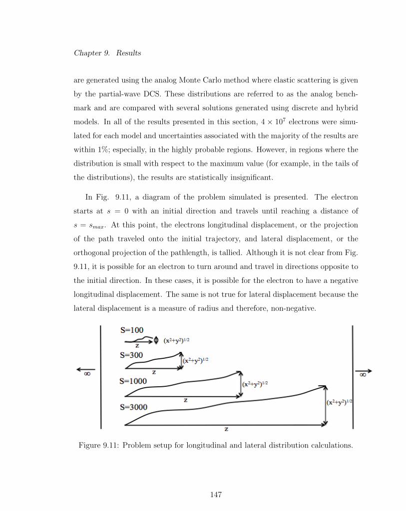
Chapter 9. Results
are generated using the analog Monte Carlo method where elastic scattering is given
by the partial-wave DCS. These distributions are referred to as the analog bench-
mark and are compared with several solutions generated using discrete and hybrid
models. In all of the results presented in this section, 4 × 10⁷ electrons were simu-
lated for each model and uncertainties associated with the majority of the results are
within 1%; especially, in the highly probable regions. However, in regions where the
distribution is small with respect to the maximum value (for example, in the tails of
the distributions), the results are statistically insignificant.
In Fig. 9.11, a diagram of the problem simulated is presented. The electron
starts at s = 0 with an initial direction and travels until reaching a distance of
s = smax. At this point, the electrons longitudinal displacement, or the projection
of the path traveled onto the initial trajectory, and lateral displacement, or the
orthogonal projection of the pathlength, is tallied. Although it is not clear from Fig.
9.11, it is possible for an electron to turn around and travel in directions opposite to
the initial direction. In these cases, it is possible for the electron to have a negative
longitudinal displacement. The same is not true for lateral displacement because the
lateral displacement is a measure of radius and therefore, non-negative.
Figure 9.11: Problem setup for longitudinal and lateral distribution calculations.
147
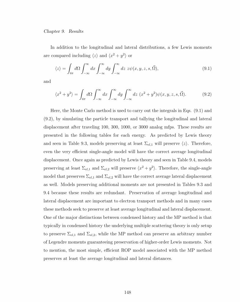
Chapter 9. Results
In addition to the longitudinal and lateral distributions, a few Lewis moments
are compared including 〈z〉 and 〈x2 + y2〉 or
〈z〉 =
∫4π
dΩ
∫ ∞−∞
dx
∫ ∞−∞
dy
∫ ∞−∞
dz zψ(x, y, z, s, ~Ω), (9.1)
and
〈x2 + y2〉 =
∫4π
dΩ
∫ ∞−∞
dx
∫ ∞−∞
dy
∫ ∞−∞
dz (x2 + y2)ψ(x, y, z, s, ~Ω). (9.2)
Here, the Monte Carlo method is used to carry out the integrals in Eqs. (9.1) and
(9.2), by simulating the particle transport and tallying the longitudinal and lateral
displacement after traveling 100, 300, 1000, or 3000 analog mfps. These results are
presented in the following tables for each energy. As predicted by Lewis theory
and seen in Table 9.3, models preserving at least Σel,1 will preserve 〈z〉. Therefore,
even the very efficient single-angle model will have the correct average longitudinal
displacement. Once again as predicted by Lewis theory and seen in Table 9.4, models
preserving at least Σel,1 and Σel,2 will preserve 〈x2 + y2〉. Therefore, the single-angle
model that preserves Σel,1 and Σel,2 will have the correct average lateral displacement
as well. Models preserving additional moments are not presented in Tables 9.3 and
9.4 because these results are redundant. Preservation of average longitudinal and
lateral displacement are important to electron transport methods and in many cases
these methods seek to preserve at least average longitudinal and lateral displacement.
One of the major distinctions between condensed history and the MP method is that
typically in condensed history the underlying multiple scattering theory is only setup
to preserve Σel,1 and Σel,2, while the MP method can preserve an arbitrary number
of Legendre moments guaranteeing preservation of higher-order Lewis moments. Not
to mention, the most simple, efficient ROP model associated with the MP method
preserves at least the average longitudinal and lateral distances.
148

Chapter 9. Results
Table 9.3: Average longitudinal displacement, 〈z〉, for 100-keV, 1000-keV, and 10000-keV electrons in copper after traveling a distance of 100, 300, 1000, and 3000 mfps.
〈z〉Pathlength
(mfps)Particle Energy
(keV) Analog 1-Angle Rel. Unc.
100100 0.8432 0.8433 0.000061000 0.986664 0.986667 0.0000110000 0.999643 0.999644 0.000001
300100 0.61815 0.61820 0.00021000 0.96069 0.96070 0.0000410000 0.998931 0.998932 0.000005
1000100 0.2761 0.2763 0.0011000 0.87673 0.87680 0.000110000 0.996449 0.996448 0.00001
3000100 0.09493 0.09497 0.0061000 0.6861 0.6863 0.000710000 0.989399 0.989387 0.00005
Table 9.4: Average lateral displacement, 〈x2+y2〉, for 100-keV, 1000-keV, and 10000-keV electrons in copper after traveling a distance of 100, 300, 1000, and 3000 mfps.
〈x2 + y2〉Physics Model
Pathlength(mfps)
Particle Energy(keV) Analog 1-Angle Rel. Unc.
100100 0.154457 0.154456 0.00031000 0.016420 0.016415 0.000810000 0.000455 0.000454 0.003
300100 0.26942 0.26944 0.00041000 0.04683 0.04682 0.000910000 0.001365 0.001364 0.004
1000100 0.2365 0.2366 0.00071000 0.1315 0.1314 0.00110000 0.0045244 0.0045245 0.0009
3000100 0.11012 0.11016 0.0021000 0.2532 0.2531 0.00110000 0.01338 0.01339 0.004
149

Chapter 9. Results
Although preservation of Σel,1 and Σel,2 guarantees preservation of 〈z〉 and
〈x2 + y2〉, resolving the longitudinal and lateral distributions(p(z, s) and p(b, s)
)respectively (see section 4.2) requires preservation of additional moments. Similar to
results from the previous section, discrete artifacts impact the shape of the longitu-
dinal and lateral distributions. The impact of the artifacts is again dependent on the
peakedness of the scattering and the number of collisions suffered by the electrons
before tallying their displacement.
In Figs. 9.12-9.17, longitudinal and lateral distributions for 10000-keV down to
100-keV electrons in an infinite copper medium are presented. Each figure contains
four results corresponding to gradually increasing pathlengths of 100, 300, 1000,
and 3000 mfps. Again, the most challenging problem, or longitudinal and lateral
distributions for 10000-keV electrons in copper, is presented first in Figs. 9.12 and
9.13. In all cases, the hybrid DCS utilized is in excellent agreement with the analog
benchmark. For shorter pathlengths, both discrete models oscillate about the analog
benchmark. The oscillations are an effect resulting from the discreteness of the DCS
model where electrons tend to travel in preferential directions. Even for pathlengths
of 1000 analog mfps, the 16-angle discrete model still oscillates subtly about the
analog benchmark, but does not for pathlengths of 3000 analog mfps.
150

Chapter 9. Results
−1 −0.8 −0.6 −0.4 −0.2 0 0.2 0.4 0.6 0.8 110
−6
10−4
10−2
100
102
z/s
P(z
/s)
Partial−wave
Discrete 4−Angles
Discrete 16−Angles
Hybrid 1−Angle, cut=0.99
(a) 100 mfp
−1 −0.8 −0.6 −0.4 −0.2 0 0.2 0.4 0.6 0.8 110
−6
10−4
10−2
100
102
z/sP
(z/s
)
Partial−wave
Discrete 4−Angles
Discrete 16−Angles
Hybrid 1−Angle, cut=0.99
(b) 300 mfp
−1 −0.8 −0.6 −0.4 −0.2 0 0.2 0.4 0.6 0.8 110
−6
10−4
10−2
100
102
z/s
P(z
/s)
Partial−wave
Discrete 4−Angles
Discrete 16−Angles
Hybrid 1−Angle, cut=0.99
(c) 1000 mfp
−1 −0.8 −0.6 −0.4 −0.2 0 0.2 0.4 0.6 0.8 110
−6
10−4
10−2
100
102
z/s
P(z
/s)
Partial−wave
Discrete 4−Angles
Discrete 16−Angles
Hybrid 1−Angle, cut=0.9
(d) 3000 mfp
Figure 9.12: Comparison of longitudinal distributions for 10000-keV electrons aftertraveling a distance of 100, 300, 1000, and 3000 analog elastic mfps in copper.
151
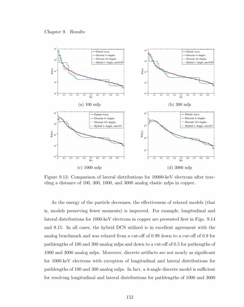
Chapter 9. Results
0 0.1 0.2 0.3 0.4 0.5 0.6 0.7 0.8 0.9 110
−6
10−4
10−2
100
102
b/s
P(b
/s)
Partial−wave
Discrete 4−Angles
Discrete 16−Angles
Hybrid 1−Angle, cut=0.99
(a) 100 mfp
0 0.1 0.2 0.3 0.4 0.5 0.6 0.7 0.8 0.9 110
−6
10−4
10−2
100
102
b/s
P(b
/s)
Partial−wave
Discrete 4−Angles
Discrete 16−Angles
Hybrid 1−Angle, cut=0.99
(b) 300 mfp
0 0.1 0.2 0.3 0.4 0.5 0.6 0.7 0.8 0.9 110
−6
10−4
10−2
100
102
b/s
P(b
/s)
Partial−wave
Discrete 4−Angles
Discrete 16−Angles
Hybrid 1−Angle, cut=0.9
(c) 1000 mfp
0 0.1 0.2 0.3 0.4 0.5 0.6 0.7 0.8 0.9 1
10−4
10−2
100
102
b/s
P(b
/s)
Partial−wave
Discrete 4−Angles
Discrete 16−Angles
Hybrid 1−Angle, cut=0.9
(d) 3000 mfp
Figure 9.13: Comparison of lateral distributions for 10000-keV electrons after trav-eling a distance of 100, 300, 1000, and 3000 analog elastic mfps in copper.
As the energy of the particle decreases, the effectiveness of relaxed models (that
is, models preserving fewer moments) is improved. For example, longitudinal and
lateral distributions for 1000-keV electrons in copper are presented first in Figs. 9.14
and 9.15. In all cases, the hybrid DCS utilized is in excellent agreement with the
analog benchmark and was relaxed from a cut-off of 0.99 down to a cut-off of 0.9 for
pathlengths of 100 and 300 analog mfps and down to a cut-off of 0.5 for pathengths of
1000 and 3000 analog mfps. Moreover, discrete artifacts are not nearly as significant
for 1000-keV electrons with exception of longitudinal and lateral distributions for
pathlengths of 100 and 300 analog mfps. In fact, a 4-angle discrete model is sufficient
for resolving longitudinal and lateral distributions for pathlengths of 1000 and 3000
152

Chapter 9. Results
analog mfps.
−0.5 0 0.5 110
−6
10−4
10−2
100
102
z/s
P(z
/s)
Partial−wave
Discrete 4−Angles
Discrete 16−Angles
Hybrid 1−Angle, cut=0.9
(a) 100 mfp
−0.8 −0.6 −0.4 −0.2 0 0.2 0.4 0.6 0.8 110
−6
10−4
10−2
100
102
z/s
P(z
/s)
Partial−wave
Discrete 4−Angles
Discrete 16−Angles
Hybrid 1−Angle, cut=0.9
(b) 300 mfp
−1 −0.8 −0.6 −0.4 −0.2 0 0.2 0.4 0.6 0.8 110
−6
10−4
10−2
100
102
z/s
P(z
/s)
Partial−wave
Discrete 4−Angles
Hybrid 1−Angle, cut=0.5
(c) 1000 mfp
−1 −0.8 −0.6 −0.4 −0.2 0 0.2 0.4 0.6 0.8 110
−6
10−4
10−2
100
102
z/s
P(z
/s)
Partial−wave
Discrete 4−Angles
Hybrid 1−Angle, cut=0.5
(d) 3000 mfp
Figure 9.14: Comparison of longitudinal distributions for 1000-keV electrons aftertraveling a distance of 100, 300, 1000, and 3000 analog elastic mfps in copper.
153

Chapter 9. Results
0 0.1 0.2 0.3 0.4 0.5 0.6 0.7 0.8 0.9 110
−6
10−4
10−2
100
102
b/s
P(b
/s)
Partial−wave
Discrete 4−Angles
Discrete 16−Angles
Hybrid 1−Angle, cut=0.99
(a) 100 mfp
0 0.1 0.2 0.3 0.4 0.5 0.6 0.7 0.8 0.9 110
−6
10−4
10−2
100
102
b/s
P(b
/s)
Partial−wave
Discrete 4−Angles
Discrete 16−Angles
Hybrid 1−Angle, cut=0.99
(b) 300 mfp
0 0.1 0.2 0.3 0.4 0.5 0.6 0.7 0.8 0.9 110
−6
10−4
10−2
100
102
b/s
P(b
/s)
Partial−wave
Discrete 4−Angles
Discrete 16−Angles
Hybrid 1−Angle, cut=0.9
(c) 1000 mfp
0 0.1 0.2 0.3 0.4 0.5 0.6 0.7 0.8 0.9 110
−6
10−4
10−2
100
102
b/s
P(b
/s)
Partial−wave
Discrete 4−Angles
Hybrid 1−Angle, cut=0.5
(d) 3000 mfp
Figure 9.15: Comparison of lateral distributions for 1000-keV electrons after travelinga distance of 100, 300, 1000, and 3000 analog elastic mfps in copper.
Finally for 100-keV electrons, the most relaxed models tested are sufficient for
pathlengths down to 100 analog mfps as seen in Figs. 9.16 and 9.17. Although
single-angle results were not presented, a single-angle model is reasonably accurate
for 100-keV electrons for pathlengths of 100 analog mfps and greater.
154

Chapter 9. Results
−1 −0.8 −0.6 −0.4 −0.2 0 0.2 0.4 0.6 0.8 110
−6
10−4
10−2
100
102
z/s
P(z
/s)
Partial−wave
Discrete 4−Angles
Hybrid 1−Angle, cut=0.5
(a) 100 mfp
−1 −0.8 −0.6 −0.4 −0.2 0 0.2 0.4 0.6 0.8 110
−6
10−4
10−2
100
102
z/sP
(z/s
)
Partial−wave
Discrete 4−Angles
Hybrid 1−Angle, cut=0.5
(b) 300 mfp
−1 −0.8 −0.6 −0.4 −0.2 0 0.2 0.4 0.6 0.8 110
−6
10−4
10−2
100
102
z/s
P(z
/s)
Partial−wave
Discrete 4−Angles
Hybrid 1−Angle, cut=0.5
(c) 1000 mfp
−1 −0.8 −0.6 −0.4 −0.2 0 0.2 0.4 0.6 0.8 110
−6
10−4
10−2
100
102
z/s
P(z
/s)
Partial−wave
Discrete 4−Angles
Hybrid 1−Angle, cut=0.5
(d) 3000 mfp
Figure 9.16: Comparison of longitudinal distributions for 100-keV electrons aftertraveling a distance of 100, 300, 1000, and 3000 analog elastic mfps in copper.
155

Chapter 9. Results
0 0.1 0.2 0.3 0.4 0.5 0.6 0.7 0.8 0.9 110
−6
10−4
10−2
100
102
b/s
P(b
/s)
Partial−wave
Discrete 4−Angles
Hybrid 1−Angle, cut=0.5
(a) 100 mfp
0 0.1 0.2 0.3 0.4 0.5 0.6 0.7 0.8 0.9 110
−6
10−4
10−2
100
102
b/s
P(b
/s)
Partial−wave
Discrete 4−Angles
Hybrid 1−Angle, cut=0.5
(b) 300 mfp
0 0.1 0.2 0.3 0.4 0.5 0.6 0.7 0.8 0.9 110
−6
10−4
10−2
100
102
b/s
P(b
/s)
Partial−wave
Discrete 4−Angles
Hybrid 1−Angle, cut=0.5
(c) 1000 mfp
0 0.1 0.2 0.3 0.4 0.5 0.6 0.7 0.8 0.9 110
−6
10−4
10−2
100
102
b/s
P(b
/s)
Partial−wave
Discrete 4−Angles
Hybrid 1−Angle, cut=0.5
(d) 3000 mfp
Figure 9.17: Comparison of lateral distributions for 100-keV electrons after travelinga distance of 100, 300, 1000, and 3000 analog elastic mfps in copper.
In this section, longitudinal and lateral results were presented to demonstrate
the effectiveness of the MP method when calculating quantities that are critical to
most CH methods and electron transport methods in general. It was shown that
the average longitudinal and lateral displacement (typically used in CH pathlength
correction algorithms) is in exact agreement with analog results for a single-angle
(two moment-preserving) model. In other words, no additional pathlength correction
algorithm is required in the MP method because the ROP DCS are constructed
such that the Lewis moments are inherently preserved. In addition, longitudinal and
lateral distributions for 100-keV (less-peaked scattering) to 10000-keV (highly-peaked
156

Chapter 9. Results
scattering) were generated using various ROP models. Depending on the problem at
hand, ROP models requiring preservation of only a few moments were required for
agreement with the analog benchmark. When necessary, additional moments were
preserved to achieve analog level accuracy, but there was never a problem too extreme
that the MP method failed to resolve the longitudinal or lateral distributions.
9.3 1-D and 2-D Dose Calculations
In this section, 1-D and 2-D dose results are presented. The dose results were gener-
ated using the partial-wave elastic scattering DCS and the Moller inelastic scattering
model for the analog benchmark and the ROP DCSs were, in turn, constructed from
these DCSs. Secondary production was not considered for this section. The fol-
lowing results show that the MP method can be used to calculate dose accurately
in both relatively isotropic and highly peaked regimes regardless of the form of the
analog model used to construct the ROP DCS. That is, accurate models can be
constructed from both analytical DCS and tabulated DCS data. In this dissertation
the emphasis is on tabulated elastic DCS data, as applications of the MP method
to analytical DCSs has been demonstrated in the past [60, 61]. Efficiency gains im-
prove significantly with increasing source energies without sacrificing accuracy. The
trade-off between accuracy and efficiency, where it exist, ultimately depends on the
application and the level of accuracy required by the user.
9.3.1 One-dimensional depth-dose profiles
Transversely integrated depth-dose profiles and relative differences are presented for
250-keV electrons in gold and 20000-keV electrons in water. In Fig. 9.18a, the re-
sults are nearly indistinguishable from the benchmark. However, Fig. 9.18b shows
157
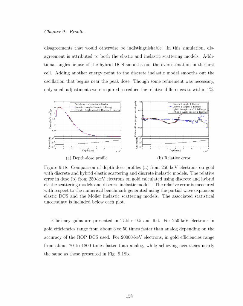
Chapter 9. Results
disagreements that would otherwise be indistinguishable. In this simulation, dis-
agreement is attributed to both the elastic and inelastic scattering models. Addi-
tional angles or use of the hybrid DCS smooths out the overestimation in the first
cell. Adding another energy point to the discrete inelastic model smooths out the
oscillation that begins near the peak dose. Though some refinement was necessary,
only small adjustments were required to reduce the relative differences to within 1%.
0
0.5
1
1.5
2
2.5
3
Dose
(M
eV
cm
2/g
)
Partial−wave expansion + Moller
Discrete 1−Angle, Discrete 1−Energy
Hybrid 1−Angle, cut=0.5, Discrete 1−Energy
0 1 2 3 4 5 6 7 8
x 10−3
10−4
10−2
100
Depth (cm)
Uncert
ain
ty
(a) Depth-dose profile
−0.1
−0.05
0
0.05
0.1
Rela
tive E
rror
(Appro
x./
Analo
g−
1)
Discrete 1−Angle, 1−Energy
Discrete 2−Angles, 2−Energies
Hybrid 1−Angle, cut=0.5, 1−Energy
Hybrid 1−Angle, cut=0.5, 2−Energies
0 1 2 3 4 5 6 7 8
x 10−3
10−4
10−2
100
Depth (cm)
Uncert
ain
ty
(b) Relative error
Figure 9.18: Comparison of depth-dose profiles (a) from 250-keV electrons on goldwith discrete and hybrid elastic scattering and discrete inelastic models. The relativeerror in dose (b) from 250-keV electrons on gold calculated using discrete and hybridelastic scattering models and discrete inelastic models. The relative error is measuredwith respect to the numerical benchmark generated using the partial-wave expansionelastic DCS and the Moller inelastic scattering models. The associated statisticaluncertainty is included below each plot.
Efficiency gains are presented in Tables 9.5 and 9.6. For 250-keV electrons in
gold efficiencies range from about 3 to 50 times faster than analog depending on the
accuracy of the ROP DCS used. For 20000-keV electrons, in gold efficiencies range
from about 70 to 1800 times faster than analog, while achieving accuracies nearly
the same as those presented in Fig. 9.18b.
158
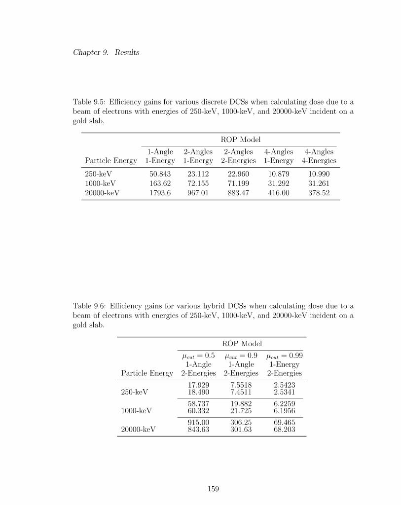
Chapter 9. Results
Table 9.5: Efficiency gains for various discrete DCSs when calculating dose due to abeam of electrons with energies of 250-keV, 1000-keV, and 20000-keV incident on agold slab.
ROP Model
Particle Energy1-Angle
1-Energy2-Angles1-Energy
2-Angles2-Energies
4-Angles1-Energy
4-Angles4-Energies
250-keV 50.843 23.112 22.960 10.879 10.9901000-keV 163.62 72.155 71.199 31.292 31.26120000-keV 1793.6 967.01 883.47 416.00 378.52
Table 9.6: Efficiency gains for various hybrid DCSs when calculating dose due to abeam of electrons with energies of 250-keV, 1000-keV, and 20000-keV incident on agold slab.
ROP Model
Particle Energy
µcut = 0.51-Angle
2-Energies
µcut = 0.91-Angle
2-Energies
µcut = 0.991-Energy
2-Energies
250-keV17.92918.490
7.55187.4511
2.54232.5341
1000-keV58.73760.332
19.88221.725
6.22596.1956
20000-keV915.00843.63
306.25301.63
69.46568.203
159

Chapter 9. Results
In Fig. 9.19a, the results are distinguishable from the benchmark at 20000-keV
because the relaxed approximations do not capture large angle scatter or large energy
losses. Once again, small refinements to the elastic and inelastic ROP scattering
models improves the accuracy of the results. As seen in Fig. 9.19b, model refinement
through preservation of additional moments reduces the relative differences to <1%.
Efficiency gains for the 20000-keV water simulation range from about 110 to 1600.
However, accuracies within 1% were achieved with models that were 650 to 700 times
more efficient than analog. Additional efficiency gains are presented in Tables 9.7
and 9.8.
0
0.5
1
1.5
2
Dose
(M
eV
cm
2/g
)
Partial−wave expansion + Moller
Discrete 1−Angle, 1−Energy
Hybrid 1−Angle, cut=0.5, 1−Energy
0 5 10 15 20 25 3010
−4
10−2
100
Depth (cm)
Uncert
ain
ty
(a) Depth-dose profile
−0.1
−0.05
0
0.05
0.1
Rela
tive E
rror
(Appro
x./
Analo
g−
1)
Discrete 1−Angle, 1−Energy
Discrete 2−Angles, 2−Energies
Hybrid 1−Angle, cut=0.5, 1−Energy
Hybrid 1−Angle, cut=0.5, 2−Energies
0 5 10 15 20 25 3010
−4
10−2
100
Depth (cm)
Uncert
ain
ty
(b) Relative error
Figure 9.19: Comparison of depth-dose profiles (a) from 20000-keV electrons on waterwith discrete and hybrid elastic scattering and discrete inelastic models. The relativeerror in dose (b) from 20000-keV electrons on water calculated using discrete andhybrid elastic scattering models and discrete inelastic models. The relative error ismeasured with respect to the numerical benchmark generated using the partial-waveexpansion elastic DCS and the Moller inelastic scattering models. The associatedstatistical uncertainty is included below each plot.
160

Chapter 9. Results
Table 9.7: Speed-up factors for various discrete DCSs when calculating dose due toa beam of electrons with energies of 250-keV, 1000-keV, and 20000-keV incident ona water slab.
ROP Model
Particle Energy1-Angle
1-Energy2-Angles1-Energy
2-Angles2-Energies
4-Angles1-Energy
4-Angles4-Energies
250-keV 54.199 30.066 24.115 14.945 11.2461000-keV 147.31 82.849 60.842 39.284 26.78120000-keV 1606.6 1121.6 709.04 612.26 292.89
Table 9.8: Efficiency gains for various hybrid DCSs when calculating dose due to abeam of electrons with energies of 250-keV, 1000-keV, and 20000-keV incident on awater slab.
ROP Model
Particle Energy
µcut = 0.51-Angle
2-Energies
µcut = 0.91-Angle
2-Energies
µcut = 0.991-Energy
2-Energies
250-keV26.03819.603
10.9449.4577
3.46173.2682
1000-keV74.28952.097
29.79924.925
8.02587.4572
20000-keV1078.5646.91
500.96380.35
118.02109.18
161

Chapter 9. Results
In addition to the single-material depth-dose profiles, an interface problem is pre-
sented. In this problem a 150-keV pencil beam of electrons is normally incident on
a gold-aluminum slab. The first 0.0004 cm of the slab is gold and the remainder of
the slab is aluminum. In Fig. 9.20, the depth-dose profiles for the analog benchmark
and a single-angle, single-energy discrete model are presented along with the relative
error in several discrete models. The interface occurs between the 4th and 5th cells;
however, there is no distinguishable error in Fig. 9.20b resulting from the interface.
As previously noted, the MP method preserves transport mechanics allowing for ex-
ponentially distributed collision sites. Clearly, boundary crossings are a non-issue for
this method and no additional algorithms are required to handle boundary crossings.
0
0.5
1
1.5
2
2.5
3
3.5
Dose
(M
eV
cm
2/g
)
Screened Rutherford + Moller
Discrete 1−Angle, Discrete 1−Energy
0 0.001 0.002 0.003 0.004 0.005 0.006 0.007 0.008 0.009 0.0110
−4
10−2
100
Depth (cm)
Uncert
ain
ty
(a) Depth-dose profile
−0.1
−0.05
0
0.05
0.1
Rela
tive E
rror
(Appro
x./
Analo
g−
1)
Discrete 1−Angle, Discrete 1−Energy
Discrete 2−Angles, Discrete 2−Energies
Discrete 4−Angles, Discrete 4−Energies
0 0.001 0.002 0.003 0.004 0.005 0.006 0.007 0.008 0.009 0.0110
−4
10−2
100
Depth (cm)
Uncert
ain
ty
(b) Relative error
Figure 9.20: Comparison of depth-dose profiles (a) from 150-keV electrons on a gold-aluminum slab with discrete elastic scattering and discrete inelastic models. Therelative error in dose (b) from 150-keV electrons on a gold-aluminum slab calculatedusing discrete and hybrid elastic scattering models and discrete inelastic models. Therelative error is measured with respect to the numerical benchmark generated usingthe partial-wave expansion elastic DCS and the Moller inelastic scattering models.The associated statistical uncertainty is included below each plot.
162
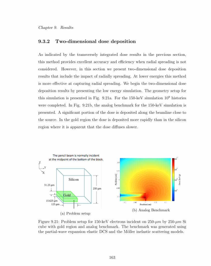
Chapter 9. Results
9.3.2 Two-dimensional dose deposition
As indicated by the transversely integrated dose results in the previous section,
this method provides excellent accuracy and efficiency when radial spreading is not
considered. However, in this section we present two-dimensional dose deposition
results that include the impact of radially spreading. At lower energies this method
is more effective at capturing radial spreading. We begin the two-dimensional dose
deposition results by presenting the low energy simulation. The geometry setup for
this simulation is presented in Fig. 9.21a. For the 150-keV simulation 109 histories
were completed. In Fig. 9.21b, the analog benchmark for the 150-keV simulation is
presented. A significant portion of the dose is deposited along the beamline close to
the source. In the gold region the dose is deposited more rapidly than in the silicon
region where it is apparent that the dose diffuses slower.
(a) Problem setup(b) Analog Benchmark
Figure 9.21: Problem setup for 150-keV electrons incident on 250-µm by 250-µm Sicube with gold region and analog benchmark. The benchmark was generated usingthe partial-wave expansion elastic DCS and the Moller inelastic scattering models.
163

Chapter 9. Results
In Fig. 9.22, relative differences for discrete models are presented to demonstrate
the impact of adjusting the number of discrete angles and energies, and in turn,
the number of moments preserved. In Figs. 9.22a and 9.22b, low-order moment-
preserving models are presented. Discrete artifacts are very distinct in in Fig. 9.22a
for the single-angle, single-energy model. By increasing the number of discrete angles
in both Figs. 9.22b and 9.22c, the discrete artifacts are mitigated without requiring
the hybrid model. However, there are still some significant differences in the dose in
some regions resulting from the single-energy model seen in Figs. 9.22b and 9.22c. By
including additional energies, the relative error in all regions is significantly reduced
as seen in Fig. 9.22d. Notice that along the gold-silicon interface near the beam, the
agreement is within 1%, with exception of the single-angle model where the solution
is overwhelmed with discrete artifacts.
Another artifact to point out is the over/under estimation of the dose in the first
two cells next to the source. This error persists as the models are refined, but it is
actually an artifact of the source type and source location. That is, the source is
a pencil beam that is singular in space and it is directed at the tally cell boundary
between. In the next 2-D result, the source is no longer singular in space and the
artifact is no longer present.
164

Chapter 9. Results
(a) 1-Angle, 1-Energy (b) 2-Angles, 1-Energy
(c) 4-Angles, 1-Energy (d) 4-Angles, 4-Energies
Figure 9.22: The relative error in dose from 150-keV electrons in a 250-µm by 250-µm Si/Au cube calculated using a discrete (a) single-angle and single-energy model,(b) two-angle and single-energy model, (c) four-angle and single-energy model, and(d) four-angle and four-energy model. The relative error is measured with respectto the numerical benchmark generated using the partial-wave expansion elastic DCSand the Moller inelastic scattering models.
165
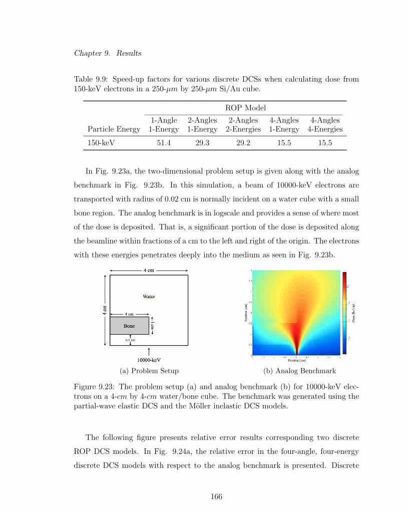
Chapter 9. Results
Table 9.9: Speed-up factors for various discrete DCSs when calculating dose from150-keV electrons in a 250-µm by 250-µm Si/Au cube.
ROP Model
Particle Energy1-Angle
1-Energy2-Angles1-Energy
2-Angles2-Energies
4-Angles1-Energy
4-Angles4-Energies
150-keV 51.4 29.3 29.2 15.5 15.5
In Fig. 9.23a, the two-dimensional problem setup is given along with the analog
benchmark in Fig. 9.23b. In this simulation, a beam of 10000-keV electrons are
transported with radius of 0.02 cm is normally incident on a water cube with a small
bone region. The analog benchmark is in logscale and provides a sense of where most
of the dose is deposited. That is, a significant portion of the dose is deposited along
the beamline within fractions of a cm to the left and right of the origin. The electrons
with these energies penetrates deeply into the medium as seen in Fig. 9.23b.
(a) Problem Setup (b) Analog Benchmark
Figure 9.23: The problem setup (a) and analog benchmark (b) for 10000-keV elec-trons on a 4-cm by 4-cm water/bone cube. The benchmark was generated using thepartial-wave elastic DCS and the Moller inelastic DCS models.
The following figure presents relative error results corresponding two discrete
ROP DCS models. In Fig. 9.24a, the relative error in the four-angle, four-energy
discrete DCS models with respect to the analog benchmark is presented. Discrete
166

Chapter 9. Results
artifacts can be seen clearly in Fig. 9.24a. However, by refining the model through
preservation of additional moments with the addition of four more discrete angles,
discrete artifacts aremitigated and backscatter is captured more accurately as seen
in the relative error result in Fig. 9.24b. In both the four-angle and eight-angle
results, no interface effects are present. It should be noted that in the backscatter is
not significant at 10000-keV and some of the error in the lower left and right corners
is statistical in nature.
(a) 4-Angles, 4-Energies (b) 8-Angles, 4-Energies
Figure 9.24: The relative error in dose from 10000-keV electrons on a 4-cm by 4-cmwater/bone cube calculated using a (a) four-angle discrete elastic DCS model andfour-energy discrete inelastic DCS model and a (b) eight-angle discrete elastic DCSmodel and four-energy discrete inelastic DCS model. The relative error is measuredwith respect to the analog benchmark generated using the partial-wave expansionelastic DCS and the Moller inelastic scattering models.
167

Chapter 9. Results
In Fig. 9.25, the relative error between the analog benchmark and two hybrid
models are presented. In Fig. 9.25a, a hybrid model with µ∗ = 0.9 shows very subtle
discrete artifacts, but otherwise is in good agreement. In Fig. 9.25b, a hybrid model
with µ∗ = 0.99 does not suffer from any discrete artifacts and the only disagreement
is in the lower left and right corners where again the error is statistical in nature.
(a) Hybrid µ∗ = 0.9, 4-Energies (b) Hybrid µ∗ = 0.99, 4-Energies
Figure 9.25: The relative error in dose from 10000-keV electrons in a 4-cm by 4-cm Water/Bone cube calculated using a (a) single-angle hybrid elastic DCS modelwith µ∗ = 0.9 and four-energy discrete inelastic DCS model and a (b) single-anglehybrid elastic DCS model with µ∗ = 0.99 elastic DCS model and four-energy discreteinelastic DCS model. The relative error is measured with respect to the analogbenchmark generated using the partial-wave expansion elastic DCS and the Mollerinelastic scattering models.
In adding more discrete angles, or through use of the hybrid model, we demon-
strated an approach to mitigate discrete artifacts through controlling the accuracy
of the ROP DCS models. The only drawback to applying a more accurate ROP DCS
model is the loss of efficiency as presented in Table 9.10. Here, the 4-angle model is
the most efficient as expected. Inclusion of additional discrete angles or use of the
hybrid model reduces the efficiency gain from roughly 120 to between 47 and 94.
As previously noted, it is possible to optimize such that significant reduction
in efficiency is not incurred by applying higher-order models in regions nearby the
168

Chapter 9. Results
Table 9.10: Speed-up factors for various discrete DCSs when calculating dose from10000-keV electrons incident on a 4-cm by 4-cm water cube with small bone region.
ROP Model
Particle Energy4-Angles
4-Energies8-Angles
4-Energies
1-Angleµ∗ = 0.9
4-Energies
1-Angleµ∗ = 0.994-Energies
10000-keV 120.7 85.6 93.9 47.0
source where the solution remains highly peaked and splaying lower-order models
in regions where the solution is less-peaked. The following results present region
dependent elastic ROP DCSs.
In Fig. 9.26, the schematic for a region dependent discrete elastic model is pre-
sented along with the associated relative error from such an approach. As seen in
Fig. 9.26a, default 4-angle, 4-energy discrete model is applied to all regions. The
default is then deactivated in the region bounded by the red dashed line and an 8-
angle, 4-energy discrete model is applied in this region. The associated relative error
is given in 9.26b. The relative error in Fig. ??b is nearly indistinguishable from the
relative error in Fig. 9.24b where an 8-angle discrete model is applied everywhere.
The resulting gain in efficiency is 106 times faster than the analog simulation as
opposed to 86 when applying an 8-angle model to all regions.
In Fig. 9.27, the schematic for another region dependent discrete elastic model
is presented along with the associated relative error from such an approach. Again,
in this problem a 4-energy discrete inelastic model is used in all regions. As seen
in Fig. 9.27a, an 8-angle model is applied in the region where the peak dose occurs
and a single-angle model is applied in all other regions. The associated relative
error is given in 9.27b and is a modest improvement over the relative error in 9.26b
as the backscatter is captured more accurately. Again, the relative error in Fig.
9.27b is nearly indistinguishable from the relative error in Fig. 9.24b where an 8-
169
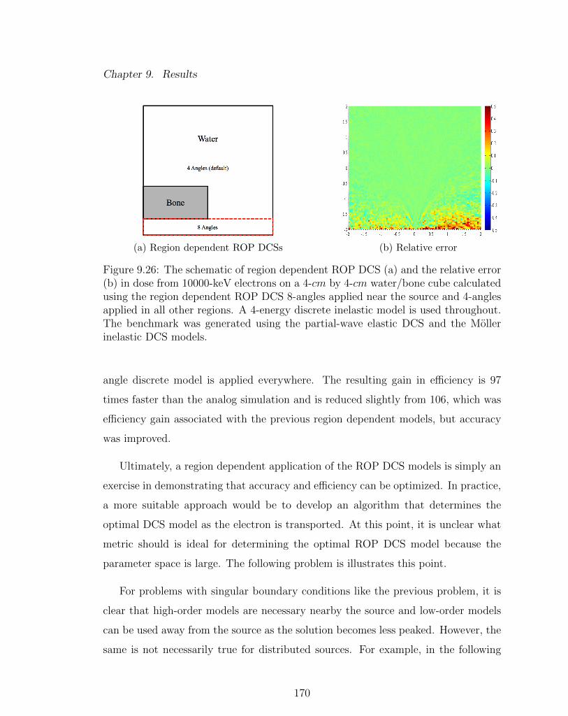
Chapter 9. Results
(a) Region dependent ROP DCSs (b) Relative error
Figure 9.26: The schematic of region dependent ROP DCS (a) and the relative error(b) in dose from 10000-keV electrons on a 4-cm by 4-cm water/bone cube calculatedusing the region dependent ROP DCS 8-angles applied near the source and 4-anglesapplied in all other regions. A 4-energy discrete inelastic model is used throughout.The benchmark was generated using the partial-wave elastic DCS and the Mollerinelastic DCS models.
angle discrete model is applied everywhere. The resulting gain in efficiency is 97
times faster than the analog simulation and is reduced slightly from 106, which was
efficiency gain associated with the previous region dependent models, but accuracy
was improved.
Ultimately, a region dependent application of the ROP DCS models is simply an
exercise in demonstrating that accuracy and efficiency can be optimized. In practice,
a more suitable approach would be to develop an algorithm that determines the
optimal DCS model as the electron is transported. At this point, it is unclear what
metric should is ideal for determining the optimal ROP DCS model because the
parameter space is large. The following problem is illustrates this point.
For problems with singular boundary conditions like the previous problem, it is
clear that high-order models are necessary nearby the source and low-order models
can be used away from the source as the solution becomes less peaked. However, the
same is not necessarily true for distributed sources. For example, in the following
170

Chapter 9. Results
(a) Region dependent ROP DCSs (b) Relative error
Figure 9.27: The schematic of region dependent ROP DCS (a) and the relative error(b) in dose from 10000-keV electrons on a4-cm by 4-cm water/bone cube calculatedusing the region dependent ROP DCS with 8-angles applied in the peak dose regionand 1-angle applied in all other regions. A 4-energy discrete inelastic model is usedthroughout. The benchmark was generated using the partial-wave elastic DCS andthe Moller inelastic DCS models.
problem an isotropic point source of 2500-keV electrons in a gold cube 1 cm on each
face is simulated. The problem setup and analog benchmark is given in Fig. 9.28.
As seen in Fig. 9.28b, the dose is deposited uniformly about the point source located
at the origin. It is also of interest to point out that most of the dose is deposited
nearby the source.
As seen in Fig. 9.29, relatively low-order models can used to estimate the dose due
to distributed sources. The most efficient model tested, single-angle, single-energy,
is about 400 times more efficient than the analog simulation and the associated
relative error is presented in Fig. 9.29a. By adding another discrete energy the
relative error improves as seen in Fig. 9.29b, but the efficiency decrease to about 300
times faster than the analog simulation. Finally, the most accurate model tested,
2-angles, 2-energies, is presented in Fig. 9.29c. This model provides good agreement,
while remaing roughly 180 times more efficient than the analog simulation. Here we
showed that accuracy and efficiency is impacted by the source configuration. Again,
171
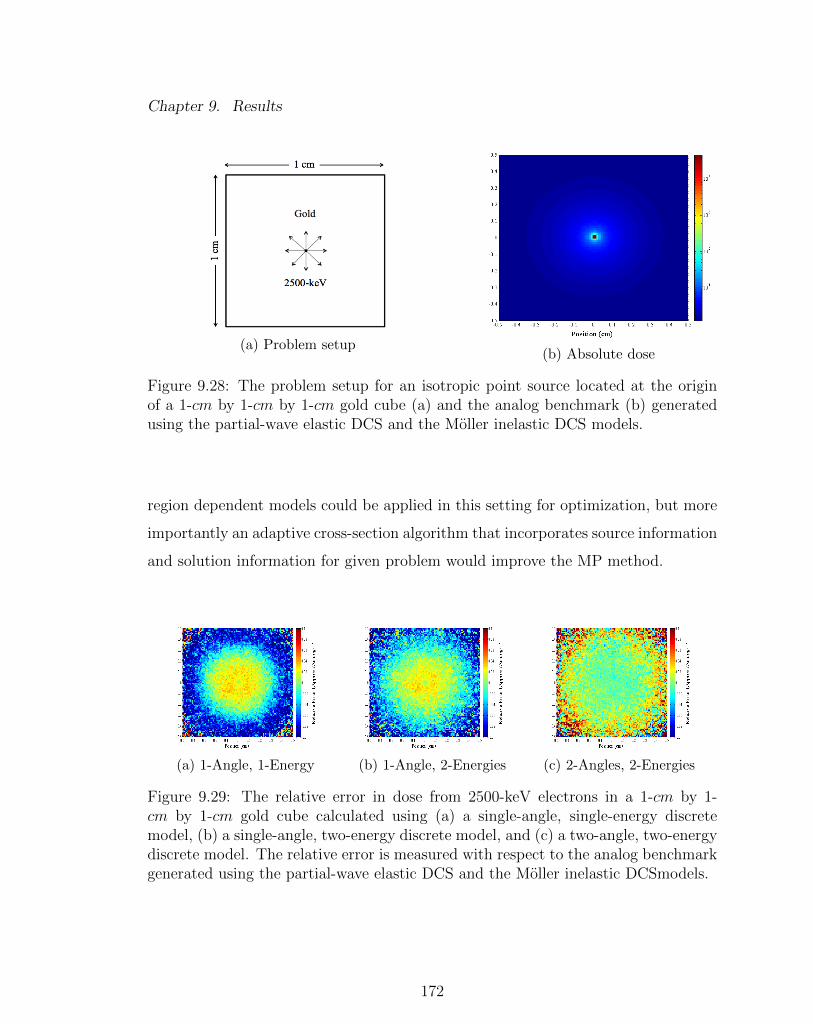
Chapter 9. Results
(a) Problem setup(b) Absolute dose
Figure 9.28: The problem setup for an isotropic point source located at the originof a 1-cm by 1-cm by 1-cm gold cube (a) and the analog benchmark (b) generatedusing the partial-wave elastic DCS and the Moller inelastic DCS models.
region dependent models could be applied in this setting for optimization, but more
importantly an adaptive cross-section algorithm that incorporates source information
and solution information for given problem would improve the MP method.
(a) 1-Angle, 1-Energy (b) 1-Angle, 2-Energies (c) 2-Angles, 2-Energies
Figure 9.29: The relative error in dose from 2500-keV electrons in a 1-cm by 1-cm by 1-cm gold cube calculated using (a) a single-angle, single-energy discretemodel, (b) a single-angle, two-energy discrete model, and (c) a two-angle, two-energydiscrete model. The relative error is measured with respect to the analog benchmarkgenerated using the partial-wave elastic DCS and the Moller inelastic DCSmodels.
172
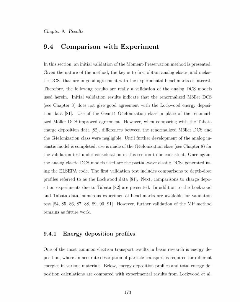
Chapter 9. Results
9.4 Comparison with Experiment
In this section, an initial validation of the Moment-Preservation method is presented.
Given the nature of the method, the key is to first obtain analog elastic and inelas-
tic DCSs that are in good agreement with the experimental benchmarks of interest.
Therefore, the following results are really a validation of the analog DCS models
used herein. Initial validation results indicate that the renormalized Moller DCS
(see Chapter 3) does not give good agreement with the Lockwood energy deposi-
tion data [81]. Use of the Geant4 G4eIonization class in place of the renomarl-
ized Moller DCS improved agreement. However, when comparing with the Tabata
charge deposition data [82], differences between the renormalized Moller DCS and
the G4eIonization class were negligible. Until further development of the analog in-
elastic model is completed, use is made of the G4eIonization class (see Chapter 8) for
the validation test under consideration in this section to be consistent. Once again,
the analog elastic DCS models used are the partial-wave elastic DCSs generated us-
ing the ELSEPA code. The first validation test includes comparisons to depth-dose
profiles referred to as the Lockwood data [81]. Next, comparisons to charge depo-
sition experiments due to Tabata [82] are presented. In addition to the Lockwood
and Tabata data, numerous experimental benchmarks are available for validation
test [84, 85, 86, 87, 88, 89, 90, 91]. However, further validation of the MP method
remains as future work.
9.4.1 Energy deposition profiles
One of the most common electron transport results in basic research is energy de-
position, where an accurate description of particle transport is required for different
energies in various materials. Below, energy deposition profiles and total energy de-
position calculations are compared with experimental results from Lockwood et al.
173

Chapter 9. Results
[81]. The Lockwood data was produced by Sandia National Laboratories using a
sophisticated calorimetric technique for measuring absolute, high-resolution electron
energy deposition profiles in a wide range of materials. The uncertainty of the data
is estimated to be from 1.0% to 2.0%.
The comparisons cover low-Z and high-Z materials including carbon, aluminum,
molybdenum, and tantalum for pencil beam sources with energies of 500-keV and
1000-keV and angles of incidence of 0 and 60. In each simulation, 105 source
particles were transported and the energy deposition profiles are normalized to the
mean CSDA range and the depth variable is in terms of a fraction of the mean CSDA
range. The primary objective of this comparison is to validate the ROP models that
are the subject of this dissertation, but also to demonstrate how well these models
perform with respect to the current state-of-art physics models available to Geant4
users. Both accuracy and efficiency results are presented, contrasting the MP method
and the default Geant4 electromagnetic physics.
Simulations were completed for three different models where the treatment of
elastic scattering varies between each model. These models include an analog elastic
scattering model given by the partial-wave DCS, a discrete single-angle DCS, and
the geant4 elastic multiple scattering model referred to as the Urban model or the
G4UrbanMscModel96 class. Each of the models tested used the same inelastic scat-
tering model and bremsstrahlung model along with the same physics for transporting
photons and positrons. The settings associated with the aforementioned physics are
in accordance with the Geant4 standard electromagnetic physics list option 3, which
was found to give the best agreement with the Lockwood data [92] and enforces the
strictest multiple scattering step limitation [93] (this is only relevant to the Urban
model). In addition, the maximum step-size was set to 0.01 mm for carbon and alu-
minum and 0.001 mm for molybdenum and tantalum when using the Urban model
(step limits are not required for the analog model or the discrete model).
174

Chapter 9. Results
In general, the energy deposition profiles calculated using the analog model, the
ROP model, and the geant4 CH model exhibit behavior similar to the experimental
results. The Geant4 physics tends to estimate values higher than the discrete model
in the peak energy deposition region, while the discrete model tends to estimate
higher values in the tails of the energy deposition profile (see Figs. 9.31-9.36). This
is true for both normal incidence and 60 off-normal incidence. The total energy
deposition tends to be nearly the same for both the MP method and the Geant4
physics models. For normally incident electrons, the agreement between all models
and the experimentally determined total energy deposition is roughly 1-3% relative
difference for all materials and energies with exception of 1000-keV electrons on
tantalum which is between roughly 4-5% (see Table 9.11). For off-normal incidence,
the agreement between all models and the experimentally determined total energy
deposition is roughly 2-4% relative difference (see Table 9.12) for all materials and
energies with exception of 1000-keV electrons on molybdenum which is between
roughly 6-7%. While this level of agreement is generally acceptable, it is of interest
to develop an analog inelastic model that improves overall agreement to within a few
percent relative error.
The timing results are presented in Tables 9.13 and 9.15. For normal incidence,
efficiency gains are roughly the same for the MP method and the Geant4 physics.
However, for off-normal incidence, the MP method is in all cases a factor of two
times faster than the Geant4 physics.
For energy deposition calculations, neither the MP method or the Geant4 physics
overwhelmingly outperform the other. However, the MP method was more efficient
for the off-normal incidence simulations. In addition, if an analog model is developed
that provides better agreement with experiment, the same level of agreement would
be anticipated for the MP method. Therefore, it is important to identify an ideal
analog inelastic model as the partial-wave DCSs are assumed to be most accurate
175

Chapter 9. Results
representation of elastic scattering and do not contribute to any disagreement found
herein.
Furthermore, no multi-region problems were validated in this section. It is known
that material interfaces are problematic for condensed history methods and there
are reported discrepancies between the Geant4 physics and the Lockwood data for
material interfaces [92]. Validation of the MP method for energy deposition in slabs
with material interfaces remains as future work, but it has been shown in the past
that the MP method does not suffer from boundary crossing limitations [60, 61, 62]
(see section 9.3). Therefore, no significant interface discrepancies are anticipated.
Table 9.11: Total energy deposition comparison for 500-keV and 1000-keV electronsnormally incident on aluminum, molybdenum, and tantalum semi-infinite slabs.
Energy(keV)
MaterialType
ModelType
Total Energy(keV)
RelativeError
500 aluminumAnalog 472.921 -0.013
Discrete 1-Angle 471.169 -0.016G4EmStandard 468.550 -0.022
1000 aluminumAnalog 958.381 -0.012
Discrete 1-Angle 954.665 -0.016G4EmStandard 953.089 -0.017
500 molybdenumAnalog 383.612 0.028
Discrete 1-Angle 381.167 0.022G4EmStandard 376.032 0.008
1000 molybdenumAnalog 801.527 0.029
Discrete 1-Angle 795.534 0.021G4EmStandard 791.940 0.017
500 tantalumAnalog 323.144 0.023
Discrete 1-Angle 316.823 0.003G4EmStandard 321.674 0.018
1000 tantalumAnalog 681.921 0.052
Discrete 1-Angle 675.622 0.043G4EmStandard 678.301 0.047
176

Chapter 9. Results
Table 9.12: Total energy deposition for 60 degrees off-normal incidence electrons onsemi-infinite slabs of aluminum, molybdenum, and tantalum.
Energy(keV)
MaterialType
ModelType
Total Energy(keV)
RelativeError
500 aluminumAnalog 380.501 -0.027
Discrete 1-Angle 379.573 -0.029G4EmStandard 375.752 -0.038
500 molybdenumAnalog 282.940 0.040
Discrete 1-Angle 279.703 0.028G4EmStandard 277.925 0.022
1000 molybdenumAnalog 597.557 0.073
Discrete 1-Angle 593.249 0.065G4EmStandard 591.644 0.062
500 tantalumAnalog 230.202 0.014
Discrete 1-Angle 226.327 -0.003G4EmStandard 232.331 0.023
1000 tantalumAnalog 493.342 0.045
Discrete 1-Angle 489.207 0.036G4EmStandard 495.368 0.050
177

Chapter 9. Results
Table 9.13: Timing results for energy deposition calculations for 500-keV and 1000-keV electrons normally incident on carbon, aluminum, molybdenum, and tantalumsemi-infinite slabs.
Energy(keV)
MaterialType
ModelType
CPU time(mins.)
EfficiencyGains
1000 carbonAnalog 75 1
Discrete 1-Angle 3 25G4EmStandard 3 25
500 aluminumAnalog 41 1
Discrete 1-Angle 3 14G4EmStandard 2 21
1000 aluminumAnalog 74 1
Discrete 1-Angle 4 19G4EmStandard 3 25
500 molybdenumAnalog 100 1
Discrete 1-Angle 2 50G4EmStandard 2 50
1000 molybdenumAnalog 151 1
Discrete 1-Angle 3 50G4EmStandard 5 30
500 tantalumAnalog 90 1
Discrete 1-Angle 2 45G4EmStandard 1 90
1000 tantalumAnalog 134 1
Discrete 1-Angle 3 45G4EmStandard 3 45
178
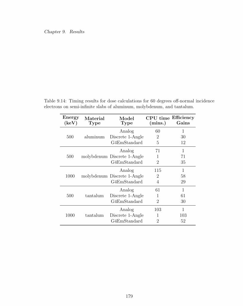
Chapter 9. Results
Table 9.14: Timing results for dose calculations for 60 degrees off-normal incidenceelectrons on semi-infinite slabs of aluminum, molybdenum, and tantalum.
Energy(keV)
MaterialType
ModelType
CPU time(mins.)
EfficiencyGains
500 aluminumAnalog 60 1
Discrete 1-Angle 2 30G4EmStandard 5 12
500 molybdenumAnalog 71 1
Discrete 1-Angle 1 71G4EmStandard 2 35
1000 molybdenumAnalog 115 1
Discrete 1-Angle 2 58G4EmStandard 4 29
500 tantalumAnalog 61 1
Discrete 1-Angle 1 61G4EmStandard 2 30
1000 tantalumAnalog 103 1
Discrete 1-Angle 1 103G4EmStandard 2 52
179
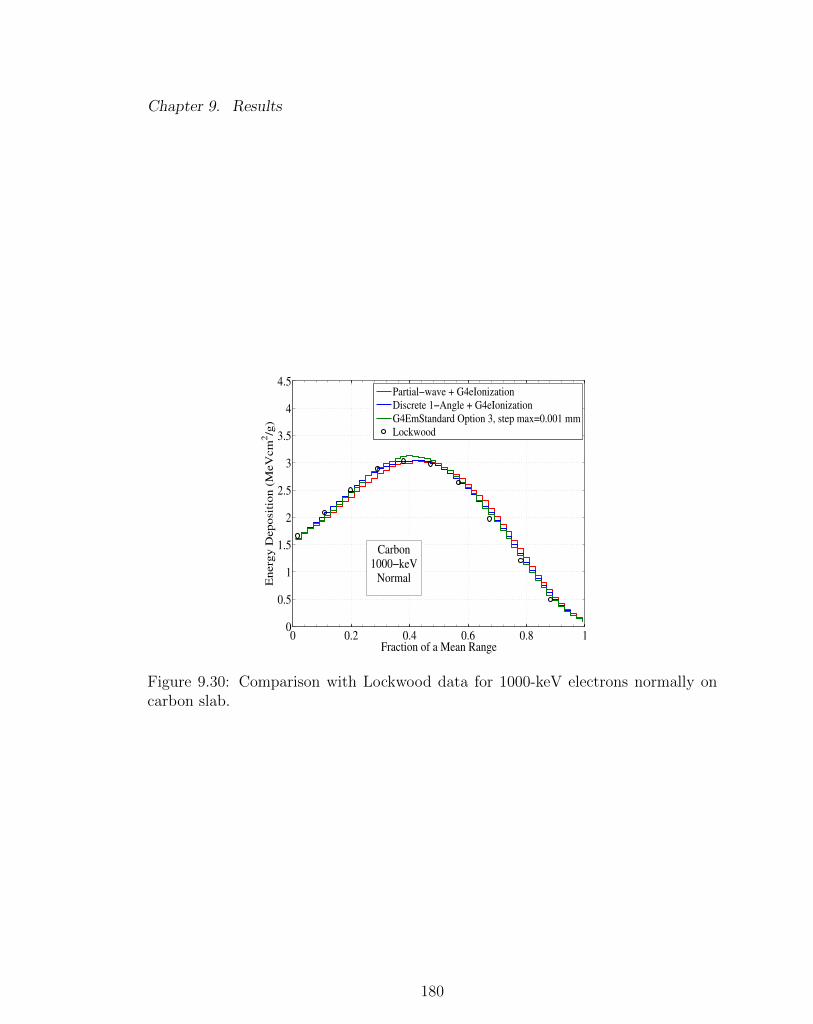
Chapter 9. Results
0 0.2 0.4 0.6 0.8 10
0.5
1
1.5
2
2.5
3
3.5
4
4.5
Fraction of a Mean Range
En
erg
y D
ep
osit
ion
(M
eV
cm
2/g
)
Partial−wave + G4eIonization
Discrete 1−Angle + G4eIonization
G4EmStandard Option 3, step max=0.001 mm
Lockwood
Carbon
1000−keV
Normal
Figure 9.30: Comparison with Lockwood data for 1000-keV electrons normally oncarbon slab.
180

Chapter 9. Results
0 0.2 0.4 0.6 0.8 10
1
2
3
4
5
6
Fraction of a Mean Range
Energ
y D
eposi
tion (
MeV
cm
2/g
)
Partial−wave + G4eIonization
Discrete 1−Angle + G4eIonization
G4EmStandard Option 3, step max=0.001 mm
Lockwood
Auminum
500−keV
Normal
(a) 500-keV
0 0.2 0.4 0.6 0.8 10
1
2
3
4
5
Fraction of a Mean Range
Energ
y D
eposi
tion (
MeV
cm
2/g
)
Partial−wave + G4eIonization
Discrete 1−Angle + G4eIonization
G4EmStandard Option 3, step max=0.001 mm
Lockwood
Aluminum
1000−keV
Normal
(b) 1000-keV
Figure 9.31: Comparison with Lockwood data for 500-keV and 1000-keV electronsnormally incident on aluminum slab.
0 0.2 0.4 0.6 0.8 10
1
2
3
4
5
Fraction of a Mean Range
Energ
y D
eposi
tion (
MeV
cm
2/g
)
Partial−wave + G4eIonization
Discrete 1−Angle + G4eIonization
G4EmStandard Option 3, step max=0.001 mm
Lockwood
Molybdenum
500−keV
Normal
(a) 500-keV
0 0.2 0.4 0.6 0.8 10
0.5
1
1.5
2
2.5
3
3.5
4
Fraction of a Mean Range
Energ
y D
eposi
tion (
MeV
cm
2/g
)
Partial−wave + G4eIonization
Discrete 1−Angle + G4eIonization
G4EmStandard Option 3, step max=0.001 mm
Lockwood
Molybdenum
1000−keV
Normal
(b) 1000-keV
Figure 9.32: Comparison with Lockwood data for 500-keV and 1000-keV electronsnormally incident on molybdenum slab.
181
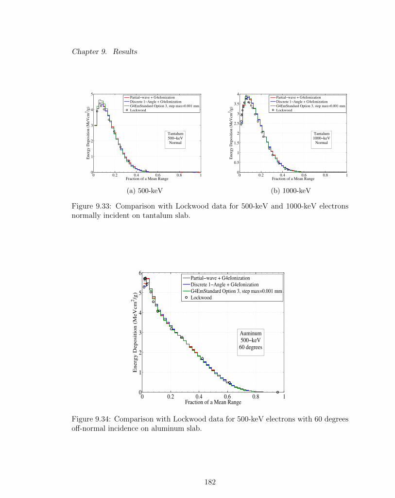
Chapter 9. Results
0 0.2 0.4 0.6 0.8 10
1
2
3
4
5
Fraction of a Mean Range
Energ
y D
eposi
tion (
MeV
cm
2/g
)
Partial−wave + G4eIonization
Discrete 1−Angle + G4eIonization
G4EmStandard Option 3, step max=0.001 mm
Lockwood
Tantalum
500−keV
Normal
(a) 500-keV
0 0.2 0.4 0.6 0.8 10
0.5
1
1.5
2
2.5
3
3.5
4
Fraction of a Mean Range
Energ
y D
eposi
tion (
MeV
cm
2/g
)
Partial−wave + G4eIonization
Discrete 1−Angle + G4eIonization
G4EmStandard Option 3, step max=0.001 mm
Lockwood
Tantalum
1000−keV
Normal
(b) 1000-keV
Figure 9.33: Comparison with Lockwood data for 500-keV and 1000-keV electronsnormally incident on tantalum slab.
0 0.2 0.4 0.6 0.8 10
1
2
3
4
5
6
Fraction of a Mean Range
En
erg
y D
ep
osit
ion
(M
eV
cm
2/g
)
Partial−wave + G4eIonization
Discrete 1−Angle + G4eIonization
G4EmStandard Option 3, step max=0.001 mm
Lockwood
Auminum
500−keV
60 degrees
Figure 9.34: Comparison with Lockwood data for 500-keV electrons with 60 degreesoff-normal incidence on aluminum slab.
182

Chapter 9. Results
0 0.2 0.4 0.6 0.8 10
1
2
3
4
5
Fraction of a Mean Range
Energ
y D
eposi
tion (
MeV
cm
2/g
)
Partial−wave + G4eIonization
Discrete 1−Angle + G4eIonization
G4EmStandard Option 3, step max=0.001 mm
Lockwood
Molybdenum
500−keV
60 degrees
(a) 500-keV
0 0.2 0.4 0.6 0.8 10
1
2
3
4
5
Fraction of a Mean Range
Energ
y D
eposi
tion (
MeV
cm
2/g
)
Partial−wave + G4eIonization
Discrete 1−Angle + G4eIonization
G4EmStandard Option 3, step max=0.001 mm
Lockwood
Molybdenum
1000−keV
60 degrees
(b) 1000-keV
Figure 9.35: Comparison with Lockwood data for 500-keV and 1000-keV electronswith 60 degrees off-normal incidence on molybdenum slab.
0 0.2 0.4 0.6 0.8 10
1
2
3
4
5
Fraction of a Mean Range
Energ
y D
eposi
tion (
MeV
cm
2/g
)
Partial−wave + G4eIonization
Discrete 1−Angle + G4eIonization
G4EmStandard Option 3, step max=0.001 mm
Lockwood
Tantalum
500−keV
60 degrees
(a) 500-keV
0 0.2 0.4 0.6 0.8 10
0.5
1
1.5
2
2.5
3
3.5
4
Fraction of a Mean Range
Energ
y D
eposi
tion (
MeV
cm
2/g
)
Partial−wave + G4eIonization
Discrete 1−Angle + G4eIonization
G4EmStandard Option 3, step max=0.001 mm
Lockwood
Tantalum
1000−keV
60 degrees
(b) 1000-keV
Figure 9.36: Comparison with Lockwood data for 500-keV and 1000-keV electronswith 60 degrees off-normal incidence on tantalum slab.
183

Chapter 9. Results
9.4.2 Charge deposition
Another important electron transport result is charge deposition. Charge deposition
is important to understanding charge buildup in nonconductive materials. Below,
charge-deposition profiles are compared with experimental results from Tabata et al.
[82]. Among the published experimental results of charge deposition distributions,
those of Tabata et al. [84] cover the widest regions of absorber atomic number (from
4 to 79) and incident-electron energy (from 4.09 to 23.5 MeV) [82].
Calculations of charge deposition distributions were performed for normally inci-
dent electron pencil beams with energies of 5000-keV, 10000-keV, and 20000-keV on
aluminum and gold targets of thickness 2.5r0, where r0 is the CSDA range. A total
of 2.4 × 10⁵ source particles were simulated. The target regions were divided into
80 sub-regions for scoring (scoring regions are not physical boundaries) for 5000-keV
source particles and 40 sub-regions for 10000-keV and 20000-keV source particles.
Particles are tracked down to 250-keV.
Figs. 9.37-9.42, present comparisons of charge-deposition and dose distributions
generated using the partial-wave elastic DCS or a discrete DCS with the default
Geant4 inelastic physics for electrons and the default Geant4 physics for positrons
and photons. The charge-deposition distributions are compared with experimen-
tal results from Tabata et al. [82]. In general the correct behavior of the charge-
deposition distribution is captured for all energies and materials tested. In alu-
minum, agreement with the experimental benchmark is satisfactory with exception
of a slight shift in the distribution. In gold, agreement with the experimental bench-
mark is again satisfactory with exception of the 5000-keV results where the charge
deposition is overestimated. Notice that the analog solution and the discrete solution
are in excellent agreement. Again, the conclusion is that an analog model that gives
good agreement should be identified and it is assumed that the ROP models will
184

Chapter 9. Results
provide similar levels of agreement. Further investigation is required to understand
the disagreements seen below (in particular, 5000-keV electrons on gold).
The dose results in Figs. 9.37-9.42, do show good agreement in gold but do not
in aluminum. This result was not anticipated considering the level of agreement in
the previous section and suggest that future validations should be avoided until this
disagreement can be identified. Possible sources of the disagreement includes the
increased presence of bremsstrahlung radiation at higher energies, an inconsistency
between the Geant4 physics implementation and discrete model, or a coding error.
Regardless, future work will include the use of an inelastic ROP model based on an
improved inelastic DCS, so that reliance on the Geant4 physics is reduced.
Table 9.15: Timing results for charge deposition calculations for 5000-keV, 10000-keV, and 20000-keV electrons normally incident on aluminum and gold semi-infiniteslabs.
Energy(keV)
MaterialType
ModelType
CPU time(mins.)
EfficiencyGains
5000 aluminumAnalog 1.6 1
Discrete 4-Angles 0.009 178Discrete 8-Angles 0.02 80
10000 aluminumAnalog 2.7 1
Discrete 4-Angles 0.01 270Discrete 8-Angles 0.03 90
20000 aluminumAnalog 5.8 1
Discrete 4-Angles 0.02 290Discrete 8-Angles 0.05 116
5000 goldAnalog 2.3 1
Discrete 4-Angles 0.03 77Discrete 8-Angles 0.06 38
10000 goldAnalog 4.3 1
Discrete 4-Angles 0.06 72Discrete 8-Angles 0.11 43
20000 goldAnalog 13.8 1
Discrete 4-Angles 0.2 69Discrete 8-Angles 0.3 46
185

Chapter 9. Results
0 0.2 0.4 0.6 0.8 1 1.2−1
−0.5
0
0.5
1
1.5
2
Scaled Depth (z/r0)
Scale
d C
harg
e D
eposi
tion (
r 0/e
)Dc
Partial−wave + G4eIonization
Discrete 4−Angles +G4eIonization
Tabata
Aluminum
5000−keV
(a) Charge Deposition
0 0.2 0.4 0.6 0.8 1 1.2 1.4 1.60
0.5
1
1.5
2
2.5
3
Depth (cm)
Dose
(M
eV
cm
2/g
)
Partial−wave + G4eIonization
Discrete 4−Angles +G4eIonization
Discrete 8−Angles +G4eIonization
(b) Dose
Figure 9.37: Comparison with Tabata data for 5000-keV electrons normally incidenton an aluminum slab.
0 0.2 0.4 0.6 0.8 1 1.2−1.5
−1
−0.5
0
0.5
1
1.5
2
2.5
Scaled Depth (z/r0)
Scale
d C
harg
e D
eposi
tion (
r 0/e
)Dc
Partial−wave + G4eIonization
Discrete 4−Angles +G4eIonization
Tabata
Aluminum
10000−keV
(a) Charge Deposition
0 0.5 1 1.5 2 2.5 30
0.5
1
1.5
2
2.5
3
Depth (cm)
Dose
(M
eV
cm
2/g
)
Partial−wave + G4eIonization
Discrete 4−Angles +G4eIonization
Discrete 8−Angles +G4eIonization
(b) Dose
Figure 9.38: Comparison with Tabata data for 10000-keV electrons normally incidenton an aluminum slab.
186

Chapter 9. Results
0 0.2 0.4 0.6 0.8 1 1.2−2
−1.5
−1
−0.5
0
0.5
1
1.5
2
2.5
Scaled Depth (z/r0)
Scale
d C
harg
e D
eposi
tion (
r 0/e
)Dc
Partial−wave + G4eIonization
Discrete 4−Angles +G4eIonization
Tabata
Aluminum
20000−keV
(a) Charge Deposition
0 1 2 3 4 5 60
0.5
1
1.5
2
2.5
3
Depth (cm)
Dose
(M
eV
cm
2/g
)
Partial−wave + G4eIonization
Discrete 4−Angles +G4eIonization
Discrete 8−Angles +G4eIonization
(b) Dose
Figure 9.39: Comparison with Tabata data for 20000-keV electrons normally incidenton an aluminum slab.
0 0.2 0.4 0.6 0.8 1 1.2−2
−1.5
−1
−0.5
0
0.5
1
1.5
2
2.5
3
Scaled Depth (z/r0)
Scale
d C
harg
e D
eposi
tion (
r 0/e
)Dc
Partial−wave + G4eIonization
Discrete 4−Angles +G4eIonization
Tabata
Gold
5000−keV
(a) Charge Deposition
0 0.05 0.1 0.15 0.20
0.5
1
1.5
2
2.5
3
3.5
Depth (cm)
Dose
(M
eV
cm
2/g
)
Partial−wave + G4eIonization
Discrete 4−Angles +G4eIonization
Discrete 8−Angles +G4eIonization
(b) Dose
Figure 9.40: Comparison with Tabata data for 5000-keV electrons normally incidenton a gold slab.
187

Chapter 9. Results
0 0.2 0.4 0.6 0.8 1 1.2−3
−2
−1
0
1
2
3
Scaled Depth (z/r0)
Scale
d C
harg
e D
eposi
tion (
r 0/e
)Dc
Partial−wave + G4eIonization
Discrete 4−Angles +G4eIonization
Tabata
Gold
10000−keV
(a) Charge Deposition
0 0.05 0.1 0.15 0.2 0.25 0.3 0.35 0.40
0.5
1
1.5
2
2.5
3
Depth (cm)
Dose
(M
eV
cm
2/g
)
Partial−wave + G4eIonization
Discrete 4−Angles +G4eIonization
Discrete 8−Angles +G4eIonization
(b) Dose
Figure 9.41: Comparison with Tabata data for 10000-keV electrons normally incidenton a gold slab.
0 0.2 0.4 0.6 0.8 1 1.2−1.5
−1
−0.5
0
0.5
1
1.5
2
Scaled Depth (z/r0)
Scale
d C
harg
e D
eposi
tion (
r 0/e
)Dc
Partial−wave + G4eIonization
Discrete 4−Angles +G4eIonization
Tabata
Gold
20000−keV
(a) Charge Deposition
0 0.1 0.2 0.3 0.4 0.5 0.6 0.70
0.5
1
1.5
2
2.5
3
Depth (cm)
Dose
(M
eV
cm
2/g
)
Partial−wave + G4eIonization
Discrete 4−Angles +G4eIonization
Discrete 8−Angles +G4eIonization
(b) Dose
Figure 9.42: Comparison with Tabata data for 20000-keV electrons normally incidenton a gold slab.
188
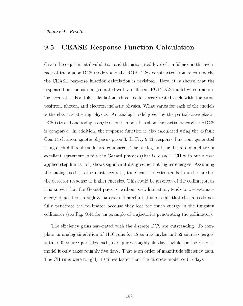
Chapter 9. Results
9.5 CEASE Response Function Calculation
Given the experimental validation and the associated level of confidence in the accu-
racy of the analog DCS models and the ROP DCSs constructed from such models,
the CEASE response function calculation is revisited. Here, it is shown that the
response function can be generated with an efficient ROP DCS model while remain-
ing accurate. For this calculation, three models were tested each with the same
positron, photon, and electron inelastic physics. What varies for each of the models
is the elastic scattering physics. An analog model given by the partial-wave elastic
DCS is tested and a single-angle discrete model based on the partial-wave elastic DCS
is compared. In addition, the response function is also calculated using the default
Geant4 electromagnetic physics option 3. In Fig. 9.43, response functions generated
using each different model are compared. The analog and the discrete model are in
excellent agreement, while the Geant4 physics (that is, class II CH with out a user
applied step limitation) shows significant disagreement at higher energies. Assuming
the analog model is the most accurate, the Geant4 physics tends to under predict
the detector response at higher energies. This could be an effect of the collimator, as
it is known that the Geant4 physics, without step limitation, tends to overestimate
energy deposition in high-Z materials. Therefore, it is possible that electrons do not
fully penetrate the collimator because they lose too much energy in the tungsten
collimator (see Fig. 9.44 for an example of trajectories penetrating the collimator).
The efficiency gains associated with the discrete DCS are outstanding. To com-
plete an analog simulation of 1116 runs for 18 source angles and 62 source energies
with 1000 source particles each, it requires roughly 46 days, while for the discrete
model it only takes roughly five days. That is an order of magnitude efficiency gain.
The CH runs were roughly 10 times faster than the discrete model or 0.5 days.
189

Chapter 9. Results
10−2
10−1
100
101
10−6
10−5
10−4
10−3
10−2
10−1
100
Energy (MeV)
R(E
) (
cm
2)
Partial−wave + Geant4 Inelastic
Discrete 1−Angle + Geant4 Inelastic
Geant4 default EM Physics Opt 3
Figure 9.43: Comparison of response functions generated using the partial-waveelastic DCS, the discrete model, the default Geant4 physics with EM option 3. Allinelastic physics, positron physics, and photon physics are the same and given bythe default Geant4 physics with EM option 3.
Figure 9.44: Electrons traversing the CEASE telescope. Collimator is in green andelectron tracks are in red.
190

Chapter 10
Conclusions and Future Work
In this chapter, the dissertation is concluded by restating the objectives of this work,
discussing what was required to satisfy the objectives, and discussing to what level
the objectives were achieved. In addition, future work is organized into several
subjects and a research pathway is considered for each subject.
10.1 Conclusions
It is of interest to develop an alternative to the CH method that is free of the limi-
tations inherent to CH. The subject of this dissertation, or the Moment-Preserving
method, is such an alternative and therefore, the accuracy and efficiency of this
method must be demonstrated and contrasted (to some degree) with the CH method.
To do so, the theoretical development of the method was discussed in great detail,
emphasizing how elements of accuracy and efficiency are inherent to the method,
while also providing an exhaustive numerical demonstration including validation of
the method.
Through theoretical development, it was shown that in the Moment-Preserving
191

Chapter 10. Conclusions and Future Work
method a reduced order physics (ROP) transport equation is formed by replacing
the analog DCS with ROP DCSs that are less-peaked with longer mfps. By doing
so, solution to the ROP transport equation using a single-event Monte Carlo method
is computationally efficient with respect to analog Monte Carlo. To simply replace
the analog DCSs with another more ideal DCS requires a process for constructing
such a DCS that guarantees accurate results. This is achieved by applying a theory
ubiquitous in electrons transport methods, or Lewis theory, that relates moments of
the analog DCS to moments of the solution. By recognizing the importance of Lewis
theory, a process was developed for constructing ROP DCSs by applying a moment-
preservation constraint, where both elastic and inelastic ROP DCSs are constructed
such that they preserve some finite number of moments of the analog DCS exactly and
higher-order moments are approximated in terms of the lower-order moments. The
resulting ROP DCSs preserve key physical moments like the mean scattering cosine,
the transport cross-section, the stopping power, and the straggling coefficient, along
with any other user specified higher-order moments. Furthermore, by constructing
the ROP DCSs such that one point is required to coincide with the nearly-singular
point of the analog DCS, the method takes advantage of a convenient cancellation
of in-scatter and out-scatter due to these nearly-singular points about zero changes-
in-state resulting in a reduction of the total cross-section. Between the moment
preserving constraint and the cancellation of the nearly-singular points, moment-
preserving ROP DCSs that are less-peaked with a longer mfp (up to four orders
of magnitude longer than the analog mfp) can be generated and accurate solutions
to the corresponding ROP transport equation can be obtained efficiently. These
findings, though satisfactory, only partially satisfy the objective of the dissertation
which is to develop and demonstrate an alternative for electron transport.
To completely satisfy the objectives, a numerical demonstration of the Moment-
Preserving method was presented. The results associated with the numerical demon-
stration, served to extend and modernize the significant body of work completed by
192

Chapter 10. Conclusions and Future Work
Franke and Prinja in 2005 [60]. By extending their study, several key features of this
method were addressed including: systematically controllable accuracy, efficiency,
mathematical robustness, versatility through the independence of the method from
the form of the analog DCS, flexibility of the method through usage of both the dis-
crete and hybrid DCS, and simplicity easing implementation in transport codes. The
accuracy and efficiency of the method was demonstrated through calculation of both
differential and integral quantities in both highly-peaked scattering regimes and less-
peaked scattering regimes for a wide variety of target materials and source energies.
Results including reflected and transmitted angular distributions and energy-loss
spectra in thin slabs, longitudinal and lateral distributions in infinite media, dose
deposition in 1-D and 2-D slabs, and charge deposition were presented. For the the-
oretical problems where the method is compared to an analog benchmark, analog
level accuracies were achieved with efficiency gains up to three orders of magni-
tude greater than analog level efficiencies. For the validation results, the accuracies
and efficiencies were similar to the default Geant4 electromagnetic physics with a
factor of two improvement in efficiency for off-normal incidence source problems. Al-
though the Moment-Preserving method was not a dramatic improvement over the
default Geant4 electromagnetic physics, this was a first attempt at validating the
method and much work remains in identifying an analog DCS model for inelastic
scattering. Improvements in accuracy beyond what was reported herein are antic-
ipated with such an inelastic DCS model. As it stands, the Moment-Preserving is
a suitable alternative; however, with these improvements one can expect that the
Moment-Preserving method will provide a clear advantage over the default Geant4
electromagnetic physics.
In its current state with regards to accuracy and efficiency, the Moment-Preserving
method is a strong alternative to CH methods. Under conditions where CH methods
and the Moment-Preserving method provide identical levels of accuracy and effi-
ciency, the Moment-Preserving method has the added advantage of versatility and
193

Chapter 10. Conclusions and Future Work
simplicity. That is, no changes to the source code or the algorithm are required to
make significant changes to the underlying physics. The moment-preserving algo-
rithms are completely independent of the form of the analog DCS that ultimately
drives the accuracy of this method. Therefore, if an improved elastic or inelastic
DCS is developed, one must simply generate an ROP DCS library corresponding to
the improved models. In addition, initial implementation of the Moment-Preserving
method is straightforward; especially, in transport codes with pre-existing single-
scatter algorithms. As a result of the mathematical robustness of the method, no
additional algorithms are required beyond what is typically used for a single-scatter
algorithm that uses tabulated DCS data. The algorithm simply requires methods
for table look-ups to obtain the total-cross section, methods for sampling DCS data
without interpolation, and methods for processing the ROP DCS. In Geant4, this
required utilization of the existing data classes and base classes for physics models
and processes. Any maintenance associated with Moment-Preserving method would
be a result of changes to the base classes from which the Moment-Preserving method
physics inherit.
Given the accuracy, efficiency, mathematical robustness, versatility, flexibility,
and simplicity of the Moment-Preserving method, this method provides a clear al-
ternative to the prevailing electron transport method - Condensed History. This
work establishes a modern basis from which further testing of this method will be
completed. This is the subject of the final section.
10.2 Future Work
Although a significant demonstration of this method was completed, further testing
and demonstration remains. Furthermore, there are other areas of work related to
this method that have not yet been investigated. This includes an adaptive cross-
194

Chapter 10. Conclusions and Future Work
section selection algorithm, extension of the method to protons and heavy ions, im-
plementation with variance reduction techniques, and countless applications. Lastly,
extension of the Moment-Preserving method for use deterministic transport codes is
an area of research where only Fokker-Planck and improved Fokker-Planck schemes
like Boltzmann Fokker-Planck and generalized Fokker-Planck methods have been
tested. Detail on each of these topics is provide below.
10.2.1 Identification of an analog model
Prior to any further work on the Moment-Preserving method, it is of interest to
identify and benchmark an analog model. As demonstrated in this work, use of
the partial-wave DCS with both renormalized Moller and the Geant4 default inelas-
tic model requires improvement. Presumably, the disagreement in the validation
results is attributed to the inelastic model because the partial-wave elastic DCSs
are the most accurate description of elastic scattering available. Therefore, what
remains is identification of an inelastic DCS model that improves agreement with
experiment. At this point, a few inelastic models have been identified including the
evaluated electron data library (EEDL) or the Livermore data [20], and the PENE-
LOPE inelastic physics that simulates inelastic collisions on the basis of a generalized
oscillator strength model [27, 94], and a modified Moller DCS [71]. What remains is
implementation and testing of the aforementioned models along with a study of the
application the moment-preserving algorithms to these inelastic models.
10.2.2 Validation
Given an analog model that provides reasonable agreement with experimental bench-
marks, it is of interest to complete a more thorough validation of the Moment-
Preserving method including further studies of energy deposition and charge depo-
195

Chapter 10. Conclusions and Future Work
sition, along with reflection, transmission, and absorption studies, and other studies
like the Fano cavity test and an external beam radiotherapy test. The following sec-
tions provide specific details on the potential validation studies along with references
to experimental benchmarks.
Energy deposition
In addition to the energy deposition validation test [81] completed herein, further
energy deposition experimental benchmarks remain. For example, several multiple-
material configurations from Lockwood et al. [81] remain unstudied which are pre-
sented in Figs. 10.1 and 10.2. In addition, Tabata et al. provided an energy-
deposition comparison [85] with several experiments for source energies ranging be-
tween 2-MeV up to 20-MeV as seen in Figs. 10.3 and 10.4. It would be insightful to
extend the scope of the validation test beyond single-material configurations and to
energies as high as 20-MeV for low-Z and high-Z materials.
(a) 500-keV (b) 1000-keV
Figure 10.1: Comparison of experimental and theoretical energy deposition profiles ina tantalum/aluminum configuration for 500 and 1000-keV electrons normally incident(fig. ref. [81]).
196

Chapter 10. Conclusions and Future Work
Figure 10.2: Comparison of experimental and theoretical energy deposition profiles inan aluminum/gold/aluminum configuration for 1000-keV electrons normally incident(fig. ref. [81]).
197

Chapter 10. Conclusions and Future Work
(a) Aluminum (b) Gold
Figure 10.3: (a) Energy-deposition distributions of 2-MeV electrons in aluminum.Line, ITS/TIGER; circles experiment by Trump et al. [95]; squares experiment byNakai et al. [96] (fig. ref. [85]). (b) Energy-deposition distributions of 2-MeVelectrons in gold. Line, ITS/TIGER; circles experiment by Aiginger and Gonauser[97] (fig. ref. [85]).
(a) 10-MeV (b) 20-MeV
Figure 10.4: Energy deposition in (a) lead for 10-MeV electrons and in (b) carbon,aluminum, and gold for 20-MeV electrons. Line, ITS/TIGER; symbols, experimentby Harder [98] (fig. ref. [85]).
198

Chapter 10. Conclusions and Future Work
Charge deposition
The charge deposition results presented in this work only included aluminum and
gold target materials. For the sake of completeness, the Moment-Preserving method
should be validated for lower-Z (like beryllium) and mid-Z (like copper and silver,
see Fig. 10.5 ) targets. Tabata et al. [82] included experimental charge deposition
results for a wide range of targets.
(a) Copper (b) Silver
Figure 10.5: Charge-depostion distributions by 5, 10, and 20 MeV electrons incidenton copper and silver. Historgrams, ITS Monte Carlo results; curves, experimentalresults obtained by the interpolation of data.
199
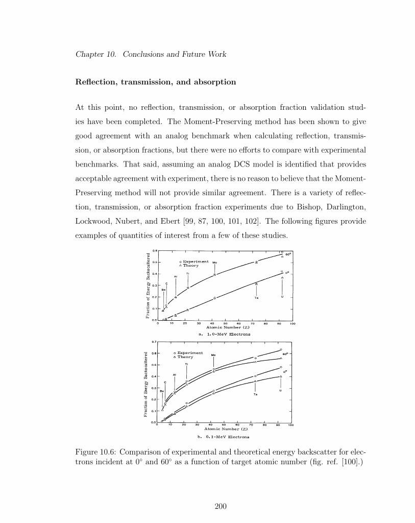
Chapter 10. Conclusions and Future Work
Reflection, transmission, and absorption
At this point, no reflection, transmission, or absorption fraction validation stud-
ies have been completed. The Moment-Preserving method has been shown to give
good agreement with an analog benchmark when calculating reflection, transmis-
sion, or absorption fractions, but there were no efforts to compare with experimental
benchmarks. That said, assuming an analog DCS model is identified that provides
acceptable agreement with experiment, there is no reason to believe that the Moment-
Preserving method will not provide similar agreement. There is a variety of reflec-
tion, transmission, or absorption fraction experiments due to Bishop, Darlington,
Lockwood, Nubert, and Ebert [99, 87, 100, 101, 102]. The following figures provide
examples of quantities of interest from a few of these studies.
Figure 10.6: Comparison of experimental and theoretical energy backscatter for elec-trons incident at 0 and 60 as a function of target atomic number (fig. ref. [100].)
200

Chapter 10. Conclusions and Future Work
Figure 10.7: Back-scattering coefficient as a function of the mass thickness of alu-minum films and gold films for different energies normally incident electrons (fig. ref.[101]).
Figure 10.8: Absorption coefficient as a function of the mass thickness of aluminumfilms and gold films for different energies normally incident electrons (fig. ref. [101]).
201

Chapter 10. Conclusions and Future Work
Fano cavity test
One of the most stringent tests for the electron transport and boundary crossing
algorithms in any condensed history Monte Carlo code is the simulation of an air
cavity as a representation of an ionization chamber [91]. The Fano cavity test (see
Fig. 10.9) is an ionization chamber test under idealized conditions such that use
can be made of the Fano Theorem [30]. That is, under charged particle equilibrium
in an infinite medium, the charged particle fluence will not be altered by density
variations from point to point. Under these conditions, a condensed history method
should agree with theoretical prediction regardless of the step-size. Ultimately, the
Fano cavity test is used to test the different mechanisms involved in CH electron
transport including step limitation, energy-loss fluctuation, and multiple scattering.
At this point, it is unclear whether or not the Fano cavity test is applicable to
the Moment-Preserving method. However, if the test is applicable it would present
an interesting comparison because the Moment-Preserving method is not step-size
dependent and does not require boundary crossing algorithms.
Figure 10.9: Fano cavity test schematic (fig. ref. [90]).
202
Chapter 10. Conclusions and Future Work
External beam radiotherapy
The last suggestion for a validation test is a comparison to the experimental results
due to Ross et al. [103] similar to work by Faddegon et al. [89]. With increased avail-
ability of Monte Carlo methods for planning electron beams, there is an increased
interest in modulated electron radiotherapy. It is imperative to determine the accu-
racy of various Monte Carlo methods for fluence and dose calculation in emerging
electron therapy treatments [89]. The accuracy of the calculated fluence distribution
may not be as accurate as calculated dose distributions. Electron therapy is generally
done using scattered electron beams and the accuracy of calculated dose distributions
is typically not as sensitive to scattered beam effects. However, calculated fluence
distributions may not be as accurate as calculated dose distributions because fluence
is sensitive to scattered beam effects. Therefore, it is important to make efforts to
validate electron transport codes against accurate measurements of fluence. Ross et
al. [103] completed such an experiment that allows a more accurate assessment of
fluence calculations. The experimental setup is presented in Fig. 10.10a, and results
from an accuracy test of EGSnrc, Geant4, and PENELOPE [89] are presented in
Fig. 10.10b.
203
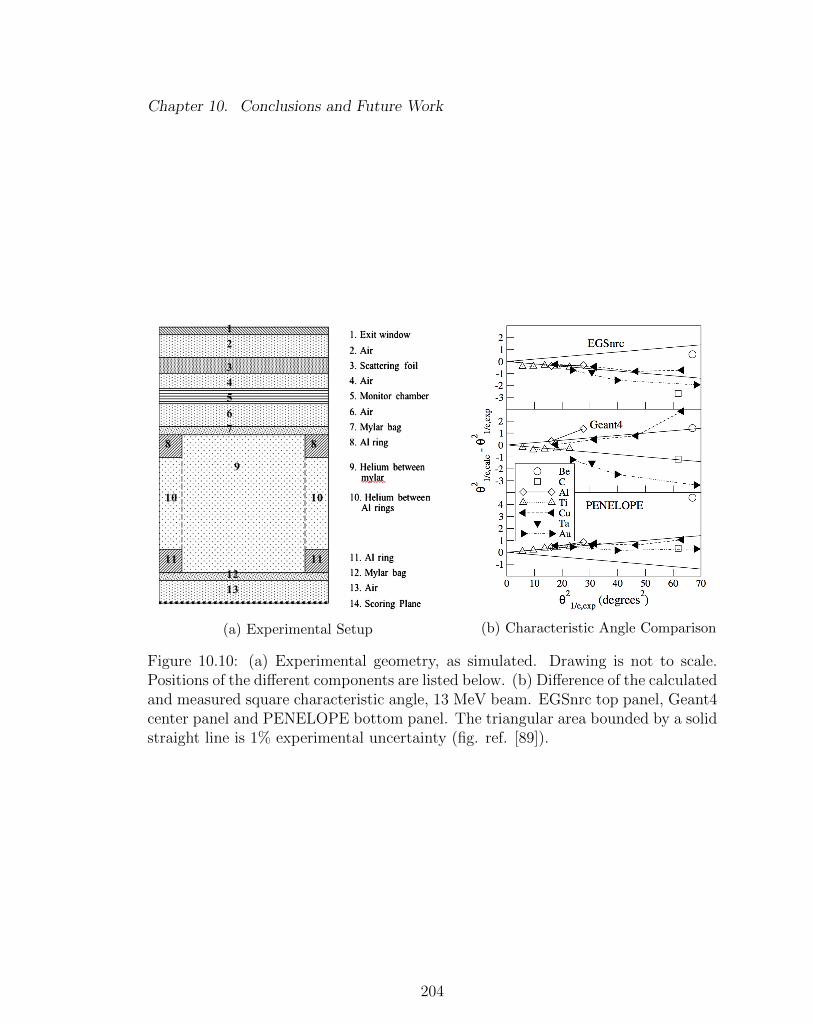
Chapter 10. Conclusions and Future Work
(a) Experimental Setup (b) Characteristic Angle Comparison
Figure 10.10: (a) Experimental geometry, as simulated. Drawing is not to scale.Positions of the different components are listed below. (b) Difference of the calculatedand measured square characteristic angle, 13 MeV beam. EGSnrc top panel, Geant4center panel and PENELOPE bottom panel. The triangular area bounded by a solidstraight line is 1% experimental uncertainty (fig. ref. [89]).
204
Chapter 10. Conclusions and Future Work
10.2.3 Adaptive cross-section selection
In section 9.3.2, 2-D dose deposition results were presented where the impact of radial
spreading is seen in the form of discrete artifacts. The discrete artifacts are mitigated
in one of two ways. That is, by adding more discrete angles to the discrete elastic
DCS or through use of the hybrid DCS with a sufficient cut, the discrete artifacts
are no longer present. As a result, the efficiency of the calculation is reduced because
more accurate representation of elastic scattering is required.
It is likely that the more accurate models are not necessary throughout the entire
calculation. For example, one could assign an ROP DCS to regions of the problem
where higher accuracy is required (for example, nearby the source) and relax the
ROP DCS in regions where lower levels of accuracy are sufficient. The selection of
the ROP DCS for each region will depend on how much information, in the form of
analog DCS moments, should be propagated from the source to the various regions
of the problem. Although interesting, this process would be tedious and is problem
dependent.
Alternatively, one could use an adaptive cross-section selection algorithm for de-
termining the ideal DCS given the initial and current state of the particle. The
metric for determining what cross-section is required is the key subject of the devel-
opment of an adaptive cross-section selection algorithm. For example, the number of
collisions suffered by the particle or the fraction of the transport mfp travelled could
be used. In addition, spatial information like longitudinal or lateral displacement
with respect to the source could be a viable metric. If such an algorithm is devel-
oped, users would not be required to select the DCS and can rely on the adaptive
cross-section selection algorithm for optimization of accuracy and efficiency.
205
Chapter 10. Conclusions and Future Work
10.2.4 Protons and heavy ions
Currently, the Moment-Preserving method has only been applied to electrons. Ex-
tension of the method to positrons is trivial and simply requires the necessary analog
DCSs. However, extension to protons and heavy ions has not yet been studied. This
will require identification of an elastic and inelastic DCS like those given by Janni
or Evans [104, 19] or for a generic ion there is a DCS suggested by Boschini et al.
[105].
Given a DCS model, the moment-preserving algorithms should be tested to de-
termine if they are effective for protons and heavy ions where the peaked-ness of the
scattering is even more extreme. It is possible that the numerics could break down;
although, some testing has been completed where the screening parameter for the
screened Rutherford elastic DCS was driven to machine precision and the moment-
preserving algorithms still produced ROP DCS that passed all tests for determining
if a viable ROP DCS was generated. One last complexity, that is converting from
center-of-mass to the lab frame when using ROP DCSs for protons and heavy ions,
must be addressed.
Lastly, the algorithms for generating ROP DCSs and the Geant4 physics models
will remain unchanged for protons and heavy ions, which makes extension of the
Moment-Preserving method to additional particles straightforward.
10.2.5 Variance reduction
Variance reduction techniques are used to reduce the number of source particles; in
turn, the efficiency of a Monte Carlo calculation is improved. There are a variety
of variance reduction techniques and all of these techniques require that the physics
models do not change throughout the calculation. For this reason, variance reduc-
206
Chapter 10. Conclusions and Future Work
tion techniques can be used in conjunction with the Moment-Preserving method
because one can select a single elastic and inelastic ROP model for use throughout
the calculation.
No testing has been completed on this subject with respect to the Moment-
Preserving method. Geant4 supports some variance reduction tools like importance
sampling (or geometrical splitting and Russian roulette) and the weight window tech-
nique, so testing of variance reduction techniques in conjunction with the Moment-
Preserving method will not require further code development.
10.2.6 Deterministic methods
Various deterministic methods based on Fokker-Planck, Boltzmann Fokker-Planck,
and generalized Fokker-Planck have been implemented. However, each of these meth-
ods rely on Fokker-Planck when regularizing the singular component of the elastic
DCS. Therefore, only the transport cross section is preserved. Deterministic meth-
ods based on the Moment-Preserving method have yet been tested. It is unclear
what kernel decomposition will be required, but it is likely that a discrete or hy-
brid model will not be appropriate in deterministic settings because of the discrete
representation. However, it is possible to construct ROP models where the singular
component is regularized with a “smoothing” function. That is, one can use an ap-
proach similar to the hybrid DCS, where the tail is represented by the analog DCS
and a moment-preserving smoothing function is applied over the peaked region of
the DCS.
207

References
[1] Brautigam, et al., Compact environmental anomaly sensor (CEASE): Responsefunctions, Tech. Rep. AFRL-VS-HA-TR-2006-1030, Air Force Research Labo-ratories (March 2006).
[2] M. J. Berger, Monte Carlo calculation of the penetration and diffusion of fastcharged particles, in: Methods in Computational Physics, Vol. 1 of StatisticalPhysics, Advances in Research and Applications, Academic Press, 1963, pp.135–215.
[3] S. Agostinelli, et al., Geant4—a simulation toolkit, NIMA 506 (2003) 250–303.
[4] L. Evans, P. Bryant, LHC machine, Jinst 3.
[5] V. N. Ivanchenko, et al., Geant4 electromagnetic physics for LHC upgrade, J.Phys.: Conf. Ser. (2014) 022015.
[6] T. Aso, et al., A geant4 based simulation for proton therapy, Computing inHigh Energy Physics.
[7] H. Paganetti, et al., Clinical implementation of full Monte Carlo dose calcula-tion in proton beam therapy, Phys. Med. Biol. 53 (2008) 4825–4853.
[8] D. Brautigam, Compact environmental anomaly sensor (CEASE): Geometricfactors, Tech. Rep. AFRL-RV-HA-TR-2008-1129, Air Force Research Labora-tories (2008).
[9] M. Y. Kim, J. W. Wilson, F. A. Cucinotta, Description of transport codes forspace radiation shielding, Health Phys. 103 (2012) 621–639.
[10] E. R. Parkinson, Monte Carlo analysis of the EMP response of a random-laycable, IEEE Trans. Nucl. Sci. NS-29 (1982) 1920–1923.
208

References
[11] G. I. Bell, S. Glasstone, Nuclear Reactor Theory, Van Nostrand Reinhold Inc.,New York, 1970.
[12] L. Carter, E. Cashwell, Particle transport simulation with the Monte Carlomethod, Tech. Rep. TID 36607, Technical Information Division (1975).
[13] B. G. Carlson, Solution of the tranport equation by Sn approximations, Tech.Rep. LA 1891, Los Alamos Scientific Laboratory (1955).
[14] F. Salvat, J. M. Fernandez-Varea, S. Segui, Analog electron physics. interac-tion cross-sections, in: Advanced Monte Carlo for Radiation Physics, ParticleTransport Simulation, 2001.
[15] A. K. Prinja, Statement of work, Tech. Rep. BAA-RV-10-01, Air Force Re-search Laboratories (2011).
[16] S. M. Seltzer, An overview of ETRAN Monte Carlo methods, in: T. M. Jenk-ins, W. R. Nelson, A. Rindi (Eds.), Monte Carlo Transport of Electrons andPhotons, Vol. 38 of Ettore Majorana International Science, Physical Sciences,Plenum Press, 1988, pp. 153–181.
[17] G. Wentzel, Z. Phys. 40 (1927) 590.
[18] F. Salvat, A. Jablonski, C. J. Powell, ELSEPA—Dirac partial-wave calculationof elastic scattering of electrons and positrons by atoms, positive ions andmolecules, Comp. Phys. Comm. 165 (2005) 157–190.
[19] R. Evans, The Atomic Nucleus, tenth printing Edition, McGraw-Hill, NewYork, 1955.
[20] S. T. Perkins, D. E. Cullen, S. M. Seltzer, Tables and graphs of electron-interaction cross-sections from 10 eV to 100 GeV derived from the LLNLevaluated electron data library (EEDL), Z=1-100, Tech. Rep. UCRL-50400,University of California Radiation Laboratories (1997).
[21] MacCallum, Bull. Am. Phys. Soc. 5 (1960) 379.
[22] J. M. Fernandez-Varea, D. Liljequist, R. Raty, F. Salvat, Monte Carlo simula-tion of 0.1-100 keV electron and positron transport in solids using optical dataand partial wave methods, Nucl. Instr. Meth. B 108 (1996) 35–50.
[23] G. H. III, Recent developments in low-energy electron/photon transport formcnp6, Progress in Nuclear Science and Technology, International Conferenceon Radiation Shielding and 17th Topical Meeting of the Radiation Protectionand Shielding Division of ANS, Nara, Japan, 2012.
209
References
[24] Ivanchenko, et al., Recent improvements in geant4 electronmagnetic physicsmodeling, Progress in Nucl. Sci. Tech. 2 (2011) 898–903.
[25] A. Bielajew, F. Salvat, Improved electron transport mechanics in the PENE-LOPE Monte-Carlo model, Nucl. Instr. Meth. B 173 (2001) 332–343.
[26] W. R. Nelson, H. Hirayama, D. W. O. Rogers, The EGS4 Code System, Stan-ford Linear Accelerator Center, SLAC–265 (1985).
[27] F. Salvat, J. M. Fernandez-Varea, J. Sempau, PENELOPE-2011: A Code Sys-tem for Monte Carlo Simulation of Electron and Photon Transport, Universitatde Barcelona (July 2011).
[28] W. Bothe, Handbuch der Physik 22 (1933) 1.
[29] B. Rossi, High Energy Particles, Prentice-Hall, Englewood Cliffs, New Jersey,1952.
[30] U. Fano, Degredation and range straggling of high-energy radiations, Phys.Rev. 92 (1953) 328.
[31] R. D. Birkhoff, Handbuch der Physik 34 (1958) 53.
[32] S. Goudsmit, J. L. Saunderson, Multiple scattering of electrons, Phys. Rev. 57(1940) 24–29.
[33] S. Goudsmit, J. L. Saunderson, Multiple scattering of electrons. ii, Phys. Rev.58 (1940) 36–42.
[34] L. Landau, On the energy loss of fast particles by ionization, J. Phys. 8 (1944)201.
[35] P. V. Vavilov, Ionization losses of high-energy heavy particles, Sov. Phys. JETP5 (4) (1957) 920–923.
[36] D. W. O. Rogers, A. F. Bielajew, A comparison of EGS and ETRAN, in:T. M. Jenkins, W. R. Nelson, A. Rindi (Eds.), Monte Carlo Transport of Elec-trons and Photons, Vol. 38 of Ettore Majorana International Science, PhysicalSciences, Plenum Press, 1988, pp. 323–342.
[37] S. M. Seltzer, M. J. Berger, Transmission and reflection of electrons by foils,Nucl. Instr. Meth. 119 (1974) 157.
[38] D. W. O. Rogers, Low energy electron transport with egs, Nucl. Instr. Meth.A A227 (1984) 535.
210
References
[39] E. W. Larsen, Generalized Fokker-Planck approximations of particle transportwith highly forward-peaked scattering, Ann. Nucl. Energy 19 (1992) 701–714.
[40] A. Bielajew, D. D. O. Rogers, PRESTA: The parameter reduced electron-steptransport algorithm for electron Monte Carlo transport, Nucl. Instr. Meth. B18 (1986) 165–181.
[41] D. Jensen, Monte Carlo calculation of electron multiple scattering in thin foils,Ph.D. thesis, Naval Postgraduate School (1988).
[42] R. L. Keith, R. P. Kensek, Order-of-convergence study of a condensed-histroyalgorithm implementation, in: International Conference on Mathematics, Com-putational Methods and Reactor Physics 2009, American Nuclear Society,Saratoga Springs, New York, 2009, on CD-ROM.
[43] H. W. Lewis, Multiple scattering in an infinite medium, Phys. Rev. 78 (1950)526–529.
[44] A. K. Prinja, Lewis theory for energy straggling in thin layers, Nucl. Instr.Meth. B 330 (2014) 99–102.
[45] G. C. Pomraning, The Fokker-Planck operator as an asymptotic limit, Math.Mod. Meth. Appl. Sci. 2 (1992) 21–36.
[46] C. Borgers, E. Larsen, Fokker-Planck approximation of monoenergetic trans-port processes, Trans. Am. Nucl. Soc. 71 (1994) 235–236.
[47] P. A. Haldy, J. Ligou, A multigroup formalism to solve the Fokker-Planckequation characterizing charged particl transport, Nucl. Sci. Eng. 74 (1980)178–184.
[48] T. M. Tran, J. Ligou, An accurate numerical method to solve the linearFokker-Planck equation characterizing charged particle transport, Nucl. Sci.Eng. 79 (269-277).
[49] J. E. Morel, Fokker-Planck calculations using standard discrete ordinates trans-port codes, Nucl. Sci. Eng. 79 (1981) 340–356.
[50] J. E. Morel, An improved Fokker-Planck angular differencing scheme, Nucl.Sci. Eng. 89 (1985) 131–136.
[51] J. Ligou, Fusion reaction product transport in inertially confined plasmas,in: Proc. ANS-ENS Int. Topl. Mtg, Advances in Mathematical Methods forthe Solution of Nuclear Engineering Problems, Fachinformationszentrum En-ergie,Physik, Mathematik GmbH, Karlsruhe, West Germany, 1981.
211

References
[52] K. Przybylski, J. Ligou, Numerical analysis of the Boltzmann equation includ-ing Fokker-Planck terms, Nucl. Sci. Eng. 81 (1981) 92–109.
[53] M. Caro, J. Ligou, Treatment of scattering anisotropy of neutrons through theBoltzmann-Fokker-Planck equation, Nucl. Sci. Eng. 83 (1983) 242–252.
[54] M. Landesman, J. E. Morel, Angular Fokker-Planck decomposition and repre-sentation techniques, Nucl. Sci. Eng. 103 (1989) 1–11.
[55] D. P. Sloan, A new multigroup Monte Carlo scattering algorithm for neutraland charged-particle Boltzmann and Fokker-Planck calculations, Tech. Rep.SAND83-7094, Sandia National Laboratories (1983).
[56] J. E. Morel, L. J. Lorence, Jr., R. P. Kensek, J. A. Hableib, D. P. Sloan,A hybrid multigroup/continuous-energy Monte Carlo method for solving theBoltzmann-Fokker-Planck equation, Nucl. Sci. Eng. 124 (1996) 369–389.
[57] G. C. Pomraning, Higher order Fokker-Planck operators, Nucl. Sci. Eng. 124(1996) 390–397.
[58] A. K. Prinja, G. Pomraning, A generalized Fokker-Planck model for transportof collimated beams, Nucl. Sci. Eng. 137 (2001) 227–235.
[59] C. L. Leakas, E. W. Larsen, Generalized Fokker-Planck approximations ofparticle transport with highly forward-peaked scattering, Nucl. Sci. Eng. 137(2001) 236–250.
[60] B. C. Franke, A. K. Prinja, Monte Carlo electron dose calculations using dis-crete scattering angles and discrete energy losses, Nucl. Sci Eng. 149 (2005)1–22.
[61] D. Dixon, A. K. Prinja, B. C. Franke, Geant4 implementation of a novel single-event Monte Carlo method for electron dose calculations, Trans. Am. Nucl. Soc.
[62] D. Dixon, A. K. Prinja, B. C. Franke, Application of the generalized BoltzmannFokker-Planck method to electron partial-wave expansion elastic scatteringdifferential cross sections within the geant4 toolkit, in: RPSD 2014, RadiationProtection and Shileding Division of the ANS, Knoxville, Tennessee, 2014.
[63] B. C. Franke, A. K. Prinja, R. P. Kensek, L. J. Lorence, Discrete scattering-angle model for electron pencil beam transport, Trans. Am. Nucl. Soc. 86(2002) 206–208.
212

References
[64] B. C. Franke, A. K. Prinja, R. P. Kensek, L. J. Lorence, Ray effect mitigationfor electron transport with discrete scattering-angles, Trans. Am. Nucl. Soc.87 (2002) 133–135.
[65] ICRU Report No. 77, Elastic scattering of electrons and positrons, Journal ofICRU 7.
[66] G. Moliere, Theori der streuung schneller geladener teilchen i: Einzelstreuungam abgeschirmten coulomb-field, Z. Naturforsch. 2a (1947) 133.
[67] Overview of physical interaction models for photon and electron transport usedin Monte Carlo codes, Metrologia 46 (2009) S112–S138.
[68] R. M. Sternheimer, Phys. Rev. (1971) 3681.
[69] ICRU Report No. 37, Stopping powers for electrons and positrons, Journal ofICRU.
[70] A. K. Prinja, E. W. Larsen, Handbook of Nuclear Engineering, Springer, 2010,Ch. Principles of Neutron Transport.
[71] M. J. Berger, R. Wang, Multiple-scattering angular deflectionsand energy-lossstraggling, in: T. M. Jenkins, W. R. Nelson, A. Rindi (Eds.), Monte CarloTransport of Electrons and Photons, Vol. 38 of Ettore Majorana InternationalScience, Physical Sciences, Plenum Press, 1988, pp. 21–56.
[72] O. Blunck, S. Leisegang, Zum energieverlustschneller elektronen in dunnenschichten, Z. Phys. 128 (1950) 500.
[73] J. A. Halbleib, R. P. Kensek, T. A. Mehlhorn, G. D. Valdez, S. M. Seltzer,M. J. Berger, ITS Version 3.0: The Integrated TIGER Series of CoupledElctron/ Photon Monte Carlo Transport Codes, Sandia National Laborato-ries, SAND91–1634 (1992).
[74] B. C. Franke, Private communication (November 2014).
[75] L. Urban, A model for multiple scattering in geant4, Tech. rep., CERN (2006).
[76] L. Harding, Monte Carlo simulatinos of electron and positron energy-loss strag-gling, Master’s thesis, University of New Mexico (2006).
[77] W. Gautschi, Numerical Analysis, second ed. Edition, Birkhauser, New York,2012.
[78] G. H. Golub, Some modified matrix eigenvalue problems, SIAM Rev. 15 (2)(1973) 318–334.
213
References
[79] G. H. Golub, J. H. Welsch, Questions of numerical condition related to orthog-onal polynomials, Studies in Numerical Analysis 24 (1984) 140–177.
[80] G. H. Golub, J. H. Welsch, Caculation of Gauss quadrature rules, Math. Comp.23 (106) (1969) 221–230.
[81] G. J. Lockwood, L. E. Ruggles, G. H. Miller, J. A. Halbleib, Calorimetricmeasurement of electron energy deposition in extended media– theory vs ex-periment, Tech. Rep. SAND79-0414, SNL (1987).
[82] T. Tabata, P. Andreo, K. Shinoda, R. Ito, Depth profiles of charge deposi-tion by electrons in elemental absorbers: Monte Carlo results, experimentalbenchmarks and derived parameters, Nucl. Instr. Meth. B 95 (1995) 289–299.
[83] E. Benedito, J. M. Fernandez-Varea, F. Salvat, Mixed simulation of the multi-ple elastic scattering of electrons and positrons using partial-wave differentialcross-sections, Nucl. Instr. Meth. B 174 (2001) 91–110.
[84] T. Tabata, R. Ito, S. Okabe, Y. Foujita, Charge distribution produced by 4- to24-MeV electrons in elemental materials, Phys. Rev. B 3 (3) (1971) 572–583.
[85] T. Tabata, P. Andreo, R. Ito, Energy-deposition distributions in materialsirradiated by plane-parallel electron beams with energies between 0.1 and 100MeV, Atomic Data and Nuclear Data Tables 56 (1994) 105–131.
[86] T. Tabata, P. Andreo, K. Shinoda, R. Ito, Range distributions and projectedranges of 0.1 to 100-MeV electrons in elemental absorbers, Nucl. Instr. Meth.B 108 (1996) 11–17.
[87] E. H. Darlington, Backscattering of 10-100 keV electrons from thick targets, J.Phys. D: Appl. Phys. 8 (1975) 85–93.
[88] P. Libby, G. Hughes III, J. Goorley, Electron transmission and backscatter ver-ification calculations using mcnp5, Tech. Rep. LA-UR-03-5751, LANL (2003).
[89] B. A. Faddegon, et al., Accuracy of EGSnrc, Geant4, and PENELOPE MonteCarlo systems for simulation of electron scattering in external beam radiother-apy, Phys. Med. Biol. 54 (2009) 6151–6163.
[90] S. Elles, V. N. Ivanchenko, M. Maire, L. Urban, Geant4 and fano cavity test:where are we?, J. Phys.: Conf. Ser. 102 (012009).
[91] E. Poon, J. Seuntjens, F. Verhaegen, Consistency test of the electron transportalgorithm in the geant4 Monte Carlo code, Phys. Med. Biol. 50 (2005) 681–694.
214
References
[92] O. Kadri, V. N. Ivanchenko, F. Gharbi, A. Trabelsi, Geant4 simulation ofelectron energy deposition in extended media, Nucl. Instr. Meth. B 258 (2007)381–387.
[93] V. N. Ivanchenko, O. Kadri, M. Maire, L. Urban, Geant4 models for simulationof multiple scattering, J. Phys.: Conf. Ser. 219 (032045).
[94] J. M. Fernandez-Varea, R. Mayol, D. Liljequist, F. Salvat, Inelastic scatteringof electrons in solids from a generalized oscillator strength model using opticaland photoelectric data, J. Phys. 5 (1993) 3593–3610.
[95] J. G. Trump, K. A. Wright, A. M. Clarke, Phys. Rev. 21 (1950) 345.
[96] Y. Nakai, Jpn. J. Appl. Phys. 2 (1963) 743.
[97] H. Aiginger, E. Gonauser, Atomkernenergic 13 (1968) 33.
[98] D. Harder, in: H. G. Ebert (Ed.), 2nd Symposium on Microdosimetry, Stresa,1969., Euratom, Brussels, 1969, p. 567.
[99] H. E. Bishop, A Monte Carlo calculation on the scattering of electrons incopper, Proc. Phys. Soc. 85 (1965) 855–866.
[100] G. J. Lockwood, L. E. Ruggles, G. H. Miller, J. A. Halbleib, Electron energyand charge albedos - calorimetric measurement vs Monte Carlo theory, Tech.Rep. SAND80-1968, Sandia National Laboratories (February 1980).
[101] G. Nubert, S. Rogaschewski, Measurements of the back-scattering and absorp-tion of 15–60 keV electrons for transparent solid films at various angles ofincidence, J. Phys. D: Appl. Phys. 17 (1984) 2439–2454.
[102] P. J. Ebert, A. F. Lauzon, E. M. Lent, Transmission and backscattering of4.0–12.0 MeV electrons, Phys. Rev. 183 (422–430).
[103] C. K. Ross, et al., Measurement of multiple scattering of 13 and 20 MeVelectrons by thin foils, Med. Phys. 35 (2008) 4121–4131.
[104] J. F. Janni, Energy loss, range, path length, time-of-flight, straggling, multiplescattering, and nuclear interaction probability, Atomic Data and Nuclear DataTables 27 (1982) 147–339.
[105] M. J. Boschini, et al., Nuclear and non-ionizing energy-loss for coulomb scat-tered particles from low energy up to relativistic regime in space nuclear andnon-ionizing energy-loss for coulomb scattered particles from low energy up torelativistic regime in space radiation environment, Proceedings of the ICATPPConference on Cosmic Rays for Particle and Astroparticle Physics (2010) 9–23.
215