
A computational model for the cooling phase of injection moulding of... · A computational model...
23
1 of 23 A computational model for the cooling phase of injection moulding A G Smith 1 , L C Wrobel 1 , B A McCalla 2 , P S Allan 2 and P R Hornsby 3 1 School of Engineering and Design, Brunel University, Uxbridge UB8 3PH, UK 2 Wolfson Centre for Materials Processing, Brunel University, Uxbridge UB8 3PH, UK 3 School of Mechanical and Aerospace Engineering, Queen's University Belfast, Belfast BT9 5AH, UK E-mail: [email protected]; [email protected] ; [email protected] ; [email protected] ; [email protected] Abstract This paper discusses the approaches and techniques used to build a realistic numerical model to analyse the cooling phase of the injection moulding process. The procedures employed to select an appropriate mesh and the boundary and initial conditions for the problem are discussed and justified. The final model is validated using direct comparisons with experimental results generated in an earlier study. The model is shown to be a useful tool for further studies aimed at optimising the cooling phase of the injection moulding process. Using the numerical model provides additional information relating to changes in conditions throughout the process, which otherwise could not be deduced or assessed experimentally. These results, and other benefits related to the use of the model, are also discussed in the paper. Key words: Injection moulding, continuous cooling, computational fluid dynamics PACS: 81.05.Lg, 47.11.+j, 44.05.+e, 44.15.+a
Transcript of A computational model for the cooling phase of injection moulding of... · A computational model...

1 of 23
A computational model for the cooling phase of injection moulding A G Smith1, L C Wrobel1, B A McCalla2, P S Allan2 and P R Hornsby3 1School of Engineering and Design, Brunel University, Uxbridge UB8 3PH, UK 2Wolfson Centre for Materials Processing, Brunel University, Uxbridge UB8 3PH,
UK 3School of Mechanical and Aerospace Engineering, Queen's University Belfast,
Belfast BT9 5AH, UK
E-mail: [email protected]; [email protected]; [email protected]; [email protected]; [email protected]
Abstract
This paper discusses the approaches and techniques used to build a realistic numerical
model to analyse the cooling phase of the injection moulding process. The procedures
employed to select an appropriate mesh and the boundary and initial conditions for
the problem are discussed and justified. The final model is validated using direct
comparisons with experimental results generated in an earlier study. The model is
shown to be a useful tool for further studies aimed at optimising the cooling phase of
the injection moulding process.
Using the numerical model provides additional information relating to changes in
conditions throughout the process, which otherwise could not be deduced or assessed
experimentally. These results, and other benefits related to the use of the model, are
also discussed in the paper.
Key words: Injection moulding, continuous cooling, computational fluid dynamics
PACS: 81.05.Lg, 47.11.+j, 44.05.+e, 44.15.+a
2 of 23
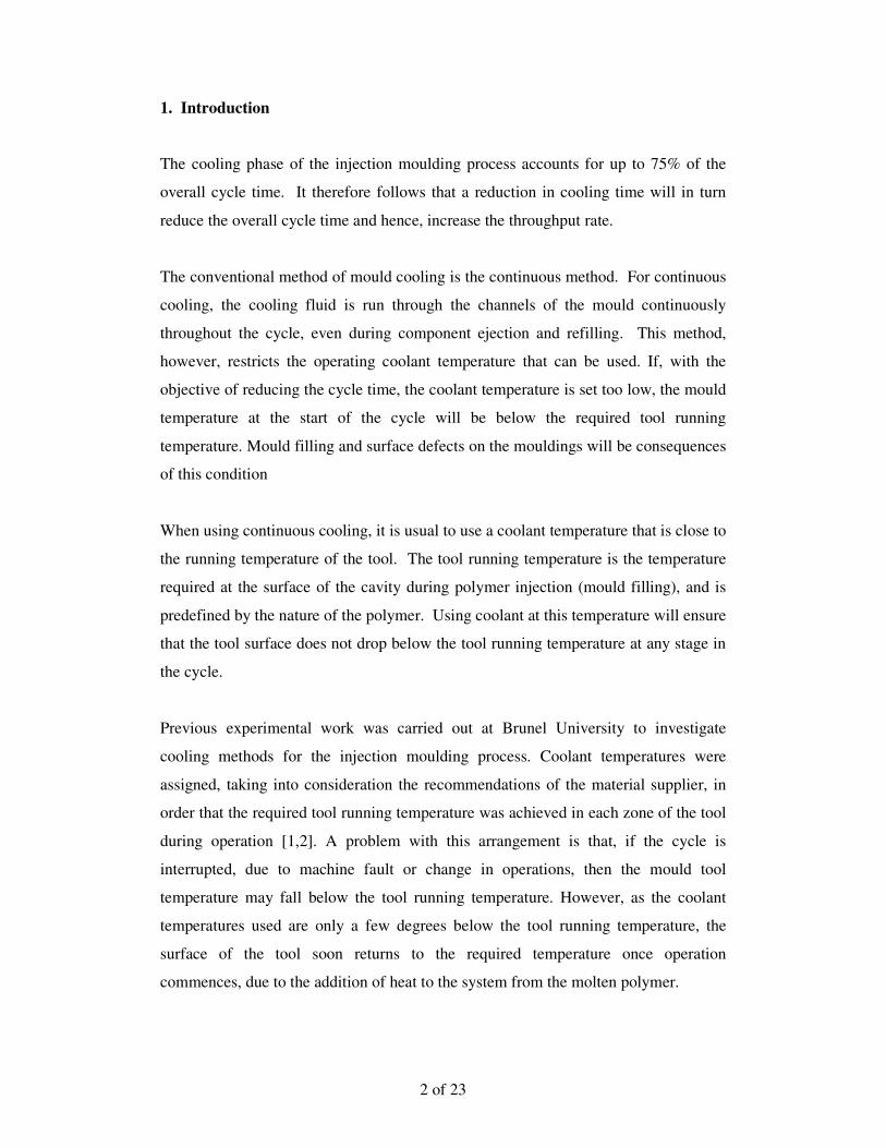
1. Introduction
The cooling phase of the injection moulding process accounts for up to 75% of the
overall cycle time. It therefore follows that a reduction in cooling time will in turn
reduce the overall cycle time and hence, increase the throughput rate.
The conventional method of mould cooling is the continuous method. For continuous
cooling, the cooling fluid is run through the channels of the mould continuously
throughout the cycle, even during component ejection and refilling. This method,
however, restricts the operating coolant temperature that can be used. If, with the
objective of reducing the cycle time, the coolant temperature is set too low, the mould
temperature at the start of the cycle will be below the required tool running
temperature. Mould filling and surface defects on the mouldings will be consequences
of this condition
When using continuous cooling, it is usual to use a coolant temperature that is close to
the running temperature of the tool. The tool running temperature is the temperature
required at the surface of the cavity during polymer injection (mould filling), and is
predefined by the nature of the polymer. Using coolant at this temperature will ensure
that the tool surface does not drop below the tool running temperature at any stage in
the cycle.
Previous experimental work was carried out at Brunel University to investigate
cooling methods for the injection moulding process. Coolant temperatures were
assigned, taking into consideration the recommendations of the material supplier, in
order that the required tool running temperature was achieved in each zone of the tool
during operation [1,2]. A problem with this arrangement is that, if the cycle is
interrupted, due to machine fault or change in operations, then the mould tool
temperature may fall below the tool running temperature. However, as the coolant
temperatures used are only a few degrees below the tool running temperature, the
surface of the tool soon returns to the required temperature once operation
commences, due to the addition of heat to the system from the molten polymer.
3 of 23
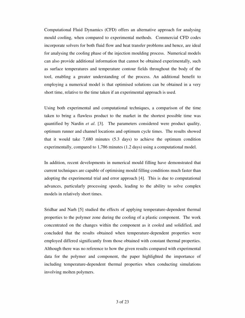
Computational Fluid Dynamics (CFD) offers an alternative approach for analysing
mould cooling, when compared to experimental methods. Commercial CFD codes
incorporate solvers for both fluid flow and heat transfer problems and hence, are ideal
for analysing the cooling phase of the injection moulding process. Numerical models
can also provide additional information that cannot be obtained experimentally, such
as surface temperatures and temperature contour fields throughout the body of the
tool, enabling a greater understanding of the process. An additional benefit to
employing a numerical model is that optimised solutions can be obtained in a very
short time, relative to the time taken if an experimental approach is used.
Using both experimental and computational techniques, a comparison of the time
taken to bring a flawless product to the market in the shortest possible time was
quantified by Nardin et al. [3]. The parameters considered were product quality,
optimum runner and channel locations and optimum cycle times. The results showed
that it would take 7,680 minutes (5.3 days) to achieve the optimum condition
experimentally, compared to 1,786 minutes (1.2 days) using a computational model.
In addition, recent developments in numerical mould filling have demonstrated that
current techniques are capable of optimising mould filling conditions much faster than
adopting the experimental trial and error approach [4]. This is due to computational
advances, particularly processing speeds, leading to the ability to solve complex
models in relatively short times.
Sridhar and Narh [5] studied the effects of applying temperature-dependent thermal
properties to the polymer zone during the cooling of a plastic component. The work
concentrated on the changes within the component as it cooled and solidified, and
concluded that the results obtained when temperature-dependent properties were
employed differed significantly from those obtained with constant thermal properties.
Although there was no reference to how the given results compared with experimental
data for the polymer and component, the paper highlighted the importance of
including temperature-dependent thermal properties when conducting simulations
involving molten polymers.
4 of 23
The objective of the work presented in this paper was to construct and validate a
computational fluid dynamics model, using continuous cooling results obtained
experimentally, in order to gain greater understanding of the cooling phase of
injection moulding, with a view to optimising the process.
2. Experimental Details and Setup
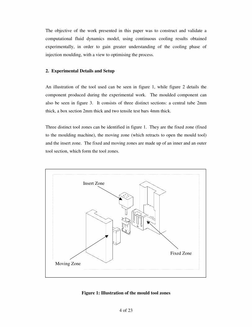
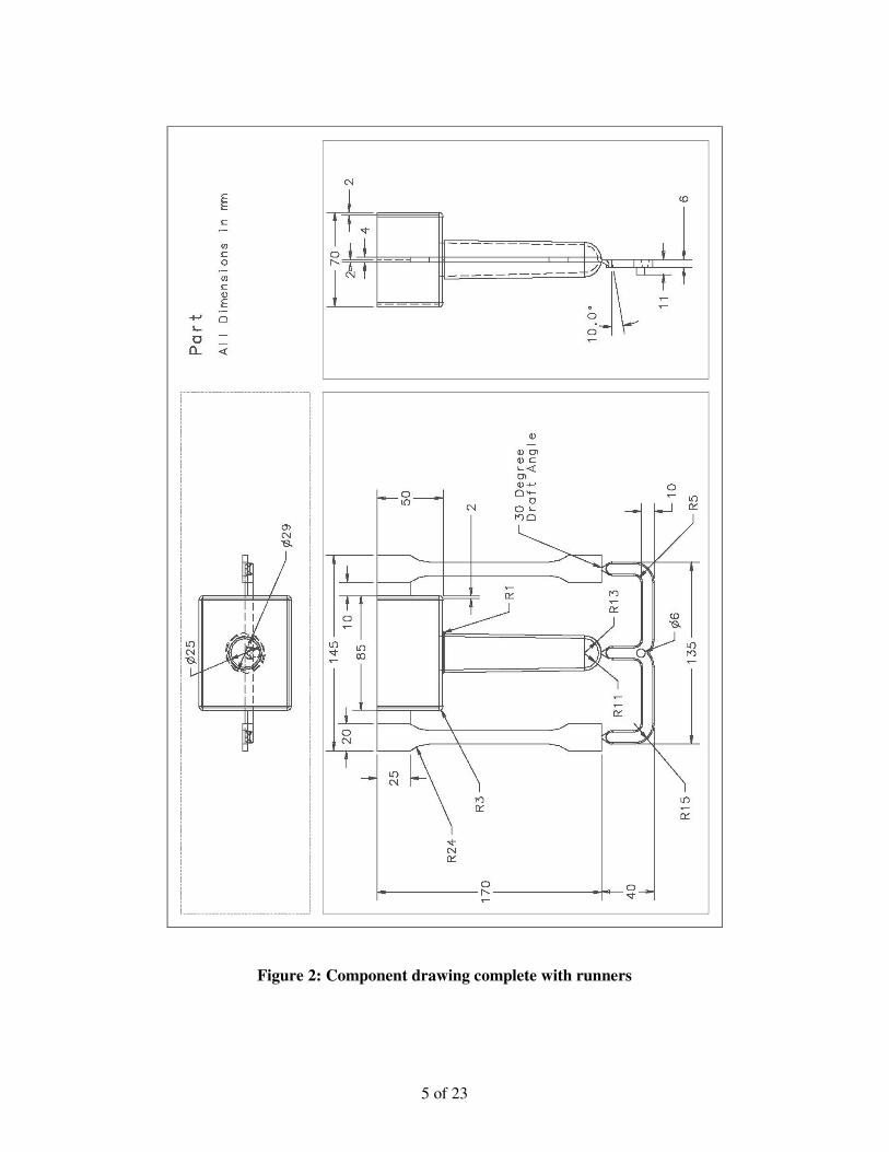
An illustration of the tool used can be seen in figure 1, while figure 2 details the
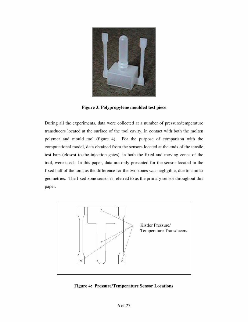
component produced during the experimental work. The moulded component can
also be seen in figure 3. It consists of three distinct sections: a central tube 2mm
thick, a box section 2mm thick and two tensile test bars 4mm thick.
Three distinct tool zones can be identified in figure 1. They are the fixed zone (fixed
to the moulding machine), the moving zone (which retracts to open the mould tool)
and the insert zone. The fixed and moving zones are made up of an inner and an outer
tool section, which form the tool zones.
Figure 1: Illustration of the mould tool zones
Moving Zone
Fixed Zone
Insert Zone
5 of 23
Figure 2: Component drawing complete with runners
6 of 23
Figure 3: Polypropylene moulded test piece
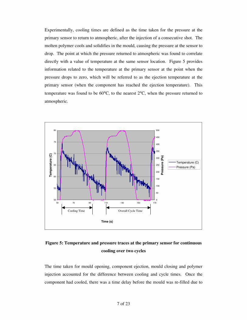
During all the experiments, data were collected at a number of pressure/temperature
transducers located at the surface of the tool cavity, in contact with both the molten
polymer and mould tool (figure 4). For the purpose of comparison with the
computational model, data obtained from the sensors located at the ends of the tensile
test bars (closest to the injection gates), in both the fixed and moving zones of the
tool, were used. In this paper, data are only presented for the sensor located in the
fixed half of the tool, as the difference for the two zones was negligible, due to similar
geometries. The fixed zone sensor is referred to as the primary sensor throughout this
paper.
Kistler Pressure/ Temperature Transducers
Figure 4: Pressure/Temperature Sensor Locations
7 of 23
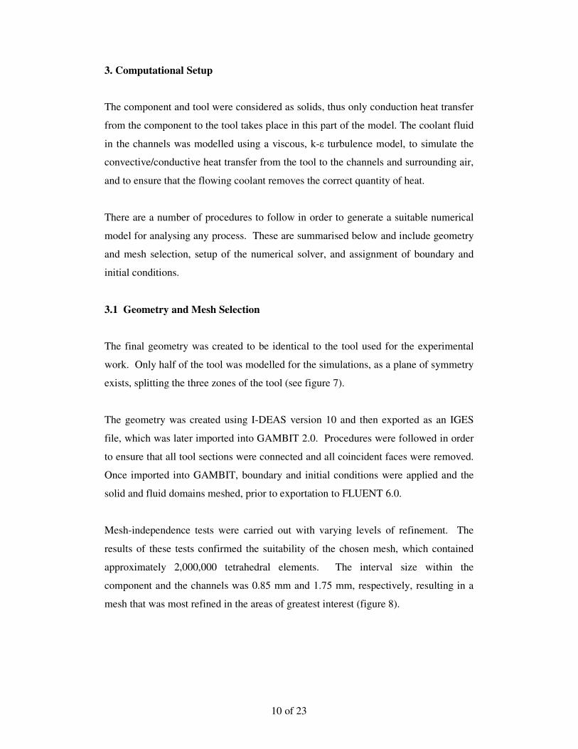
Experimentally, cooling times are defined as the time taken for the pressure at the
primary sensor to return to atmospheric, after the injection of a consecutive shot. The
molten polymer cools and solidifies in the mould, causing the pressure at the sensor to
drop. The point at which the pressure returned to atmospheric was found to correlate
directly with a value of temperature at the same sensor location. Figure 5 provides
information related to the temperature at the primary sensor at the point when the
pressure drops to zero, which will be referred to as the ejection temperature at the
primary sensor (when the component has reached the ejection temperature). This
temperature was found to be 60°C, to the nearest 2°C, when the pressure returned to
atmospheric.
50
55
60
65
70
75
80
50 70 90 110 130 150 170
Time (s)
Tem
pera
ture
(C)
0
50
100
150
200
250
300
350
400
450
500
Pre
ssur
e (P
a)Temperature (C)
Pressure (Pa)
Figure 5: Temperature and pressure traces at the primary sensor for continuous
cooling over two cycles
The time taken for mould opening, component ejection, mould closing and polymer
injection accounted for the difference between cooling and cycle times. Once the
component had cooled, there was a time delay before the mould was re-filled due to
Cooling Time Overall Cycle Time

8 of 23
these additional elements of the cycle. The overall cycle time consists of mould
filling time, cooling time and ejection time, while the objective of the computational
simulation is to analyse and reduce cooling time. Therefore, injection and ejection
times were kept constant. Multiple cycles were modelled to allow the system to
stabilise, with consistent cycle times for consecutive cycles.
All the results displayed correspond to a tool running temperature of 50˚C. The
material used was a polypropylene homopolymer, Moplen SM6100, which was
injected into the mould at a melt temperature of 220˚C. This was the temperature at
the barrel nozzle. Temperature changes due to shear effects encountered by the melt
as it was injected into the mould cavity were not evaluated.
Coolant temperatures below the tool running temperature were used in order to
prevent the tool from overheating. The coolant temperature in the fixed zone was the
lowest of the three zones, to compensate for the heat supplied by the hot runner
system. The coolant temperatures for the zones were set during moulding, based on
the temperatures recorded by the REPS AP 1/8 probe zone sensors [6] positioned
within the three zones of the tool. The coolant temperatures were adjusted until the
zone sensors gave a reading close to 50°C throughout the cycle. The locations of
these sensors, with respect to the component, can be seen in figure 6.
The coolant temperatures for the three zones that gave a corresponding tool running
temperature of 50°C were 38°C for the fixed zone, 46°C for the moving zone and
48°C for the insert zone. The temperature measured at the sensors within the fixed
and moving zones was found to fluctuate between 50°C and 52°C during each
moulding cycle, whereas the temperature fluctuated between 44°C and 57°C in the
insert zone.

9 of 23
Figure 6: Zone sensor locations in relation to the part cavity
10 of 23
3. Computational Setup
The component and tool were considered as solids, thus only conduction heat transfer
from the component to the tool takes place in this part of the model. The coolant fluid
in the channels was modelled using a viscous, k-� turbulence model, to simulate the
convective/conductive heat transfer from the tool to the channels and surrounding air,
and to ensure that the flowing coolant removes the correct quantity of heat.
There are a number of procedures to follow in order to generate a suitable numerical
model for analysing any process. These are summarised below and include geometry
and mesh selection, setup of the numerical solver, and assignment of boundary and
initial conditions.
3.1 Geometry and Mesh Selection
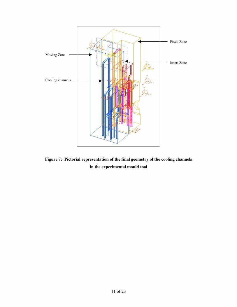
The final geometry was created to be identical to the tool used for the experimental
work. Only half of the tool was modelled for the simulations, as a plane of symmetry
exists, splitting the three zones of the tool (see figure 7).
The geometry was created using I-DEAS version 10 and then exported as an IGES
file, which was later imported into GAMBIT 2.0. Procedures were followed in order
to ensure that all tool sections were connected and all coincident faces were removed.
Once imported into GAMBIT, boundary and initial conditions were applied and the
solid and fluid domains meshed, prior to exportation to FLUENT 6.0.
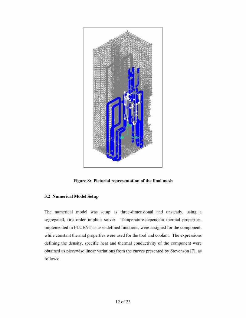
Mesh-independence tests were carried out with varying levels of refinement. The
results of these tests confirmed the suitability of the chosen mesh, which contained
approximately 2,000,000 tetrahedral elements. The interval size within the
component and the channels was 0.85 mm and 1.75 mm, respectively, resulting in a
mesh that was most refined in the areas of greatest interest (figure 8).
11 of 23
Fixed Zone Insert Zone
Moving Zone Cooling channels
Figure 7: Pictorial representation of the final geometry of the cooling channels
in the experimental mould tool
12 of 23
Figure 8: Pictorial representation of the final mesh
3.2 Numerical Model Setup
The numerical model was setup as three-dimensional and unsteady, using a
segregated, first-order implicit solver. Temperature-dependent thermal properties,
implemented in FLUENT as user-defined functions, were assigned for the component,
while constant thermal properties were used for the tool and coolant. The expressions
defining the density, specific heat and thermal conductivity of the component were
obtained as piecewise linear variations from the curves presented by Stevenson [7], as
follows:

13 of 23
Density:
8.86)50(026.077500
+−=
Tρ for 127.5˚C>T>50˚C
73.5)5.127(069.05000
+−=
Tρ for 132.5˚C>T>127.5˚C
3125.106)5.132(08.087500
+−=
Tρ for T>132.5˚C
Specific heat:
95.1170
)50( +−= TC for 90˚C>T>50˚C
1853.215
)90(3147.8 +−= TC for 105˚C>T>90˚C
5.1010
)105(1676.8 +−−= TC for 115˚C >T>105˚C
3324.2105
)115(6176.0 +−= TC for T>115˚C
Thermal conductivity:
216.075
)50(006.0 +−= TK for 125˚C >T>50˚C
222.05.7
)125(052.0 +−−= TK for 132.5˚C>T>125˚C
170.05.87
)5.132(007.0 +−= TK for T>132.5˚C
while the thermal properties of the tool and coolant are as follows:
Tool (plain carbon steel) [8]:
Density = 7,700 kg/m3
Specific heat = 460 J/kgK
Thermal conductivity = 20 W/mK
Coolant (water) [8]:
Density = 998.2 kg/m3
14 of 23
Specific heat, = 4,182 J/kgK
Thermal conductivity = 0.6 W/mK
3.3 Boundary and Initial Conditions
3.3.1 External Surfaces of the Tool
Symmetry faces were assigned a zero heat flux by default, while all other external
faces of the tool had a convective heat transfer coefficient of 15 W/m2K. This follows
information related to free and forced convection of gases over various surfaces, that
suggests a range of values between 2 and 25 W/m2K [9]. Although accurate values for
convective heat transfer coefficients can only be found experimentally, the above
value was selected because the surface of the tool was smooth and, therefore, the flow
of air within the boundary layer was not restricted by large surface asperities. In
addition, the tool itself was in a well-ventilated workshop, so air was relatively free to
flow around the tool. The free stream temperature (or temperature within the
surrounding workshop environment) was set to 27˚C.
3.3.2 Channel Inlets and Outlets
Flow in the cooling channels was simulated using a k-� turbulence model, with water
acting as the cooling fluid. One of the water heaters used on the experimental tool set-
up was a Conair 6 kW unit. These units are capable of delivering water at a nominal
rate of 95 l/min, at a pressure of 0.9 bar. Thus, the coolant velocity was calculated
using the supply pressure for the water heater pump. This value was then checked
against the nominal flow rate, to ensure that the pump was capable of delivering
coolant at the calculated velocity. It was assumed that the water pump was
responsible for elevating the water to a height of 2 metres above the height of the
pump. Using Bernoulli’s equation and neglecting losses due to friction within the
pipes gave a velocity value of 12 m/s, which was used as the channel inlet velocity.
In addition to the velocity at the inlet, the turbulence characteristics were defined
using the turbulence intensity and length scale. Using the FLUENT 6.0 User Guide
[8], the estimated values of turbulence intensity and length scale were I = 6.6% and l
= 0.07d, respectively, with d representing pipe diameter.
15 of 23
3.3.3 Solid/Fluid Interface
The solid/fluid interfaces were modeled as coupled walls, so that the values in either
zone could be evaluated and the interaction between the two could be assessed. This
condition basically assumes compatibility of temperature and velocity (in this case,
zero velocity) at the interfaces.
A simple two-dimensional simulation of flow through a channel with thick walls was
initially conducted, in order to analyse the heat transfer through the solid/fluid
interface (representative of the heat transfer between the tool and the cooling
channels). Different meshes with greater levels of refinement closer to the wall were
tested. The results showed that using a coarse mesh in the channel was normally
sufficient to accurately represent the transfer of heat from the tool to the channel,
although the flow characteristics within the channel may not be accurately
represented.
3.3.4 Initial Conditions
Initially, the tool was set at the running temperature of 50ºC and the component was
set at the polymer injection temperature of 220ºC. As the flow was transient with
consecutive shots, a repeating process was modelled with various conditions changed
throughout the simulation. The injection of a consecutive shot, once the previous
component had cooled sufficiently and reached the ejection temperature, was done
manually by temporarily interrupting the transient simulation and re-patching the
temperature in the part zone at the injection temperature of 220˚C. This manual
process was done 10 seconds after the temperature at the primary sensor reached the
ejection temperature, as this allowed sufficient time to account for tool opening, part
ejection, tool closing and polymer re-injection.
Since the purpose of this investigation was to analyse the cooling phase of the
injection moulding cycle only, the difference between cycle time and cooling time
was kept constant throughout the simulation, even though this was not the case for
some of the experimental work. Experimentally, this time ranged between 10 and 20
seconds.
16 of 23
In order to validate the numerical model, the coolant temperatures used were the same
as those used experimentally, except in the fixed zone. The coolant in the fixed zone
was at 38ºC in the experimental set-up, in order to remove the excess heat supplied by
the hot runner system. In the computational model, the coolant temperature in both
the fixed and moving zones was set at 46ºC and the coolant in the insert zone was set
at 48ºC, as the hot runners were not modelled.
4 Results and Discussion
All the results discussed in this section were used to validate the model. The data
displayed directly correlate with the data obtained experimentally, along with
additional useful data collected using the model, which could not be easily obtained
using the experimental set-up. Temperature data were collected at the sensor locations
discussed previously. In addition, data were collected relating to the minimum
temperature on the cavity surface in each zone.
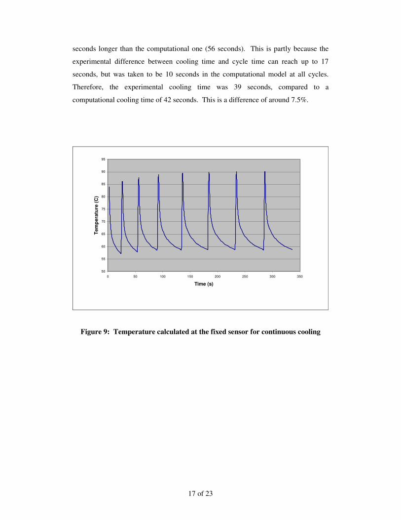
Figure 9 demonstrates that it took approximately 7 cycles for the rate of heat transfer
into and out of the tool to stabilise. Therefore, there was no net heat being taken in by
the tool, across a cycle, after this time. This represents the point at which the heat
profile throughout the tool was the same at the start and end of a cycle. Experimental
results were taken once this condition was reached, as the sample data were taken
after a large number of components had been produced.
Figure 10 looks more closely at two full cycles after the system has stabilised. It can
be seen from this figure that the overall cycle time was 52 seconds. This corresponds
to a cooling time of 42 seconds. This figure is important for the validation for the
computational model, as it graphically compares the computational and experimental
temperature readings at the primary sensor, across two complete cycles. The time
axis has been altered so that the results are in phase at the start of the first cycle for
ease of comparison.
These results are very promising as the differences between the two data sets can be
explained and justified. It can be seen that the experimental cycle time is around 4
17 of 23
seconds longer than the computational one (56 seconds). This is partly because the
experimental difference between cooling time and cycle time can reach up to 17
seconds, but was taken to be 10 seconds in the computational model at all cycles.
Therefore, the experimental cooling time was 39 seconds, compared to a
computational cooling time of 42 seconds. This is a difference of around 7.5%.
50
55
60
65
70
75
80
85
90
95
0 50 100 150 200 250 300 350
Time (s)
Tem
pera
ture
(C)
Figure 9: Temperature calculated at the fixed sensor for continuous cooling

18 of 23
30
40
50
60
70
80
90
100
0 20 40 60 80 100 120
Time from start of cycle (s)
Tem
pera
ture
(C)
Computation
Experimental
Figure 10: Comparison of computational and experimental temperature plots
over two cycles taken at the position of the primary sensor
Although relatively large differences in maximum and minimum temperatures can be
seen at the primary fixed sensors, the reasons for this are again justifiable. In the
experimental setup, the surface sensor was set into the cavity surface, therefore the
temperature of the surrounding tool also contributed to the measured temperature. In
the case of the computational model, the sensor has a negligible thickness and so an
average of the temperatures either side of the interface was reported. As the tool was
at a lower temperature than the polymer, the experimental reading was found to be
lower, as a greater proportion of the sensor was in contact with the tool.
The benefits of using a computational model should also be highlighted. It allows the
monitoring of maximum and minimum temperatures on any given surface, and also
allows the viewing of temperature contour plots on any chosen surface. This enables
the visualisation of temperature distributions throughout the tool.
Figure 11 shows a contour plot taken at the end of the final cycle. The coolant
temperatures used in each zone are given in section 3.2 and the final cycle time was
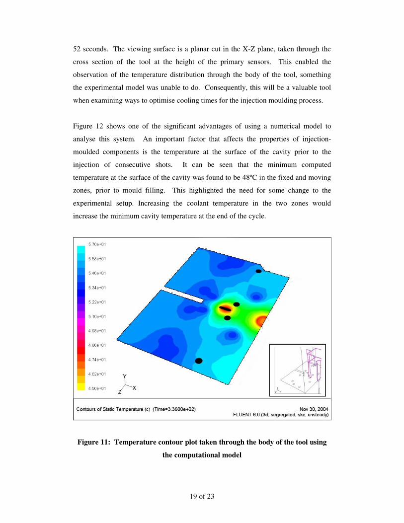
19 of 23
52 seconds. The viewing surface is a planar cut in the X-Z plane, taken through the
cross section of the tool at the height of the primary sensors. This enabled the
observation of the temperature distribution through the body of the tool, something
the experimental model was unable to do. Consequently, this will be a valuable tool
when examining ways to optimise cooling times for the injection moulding process.
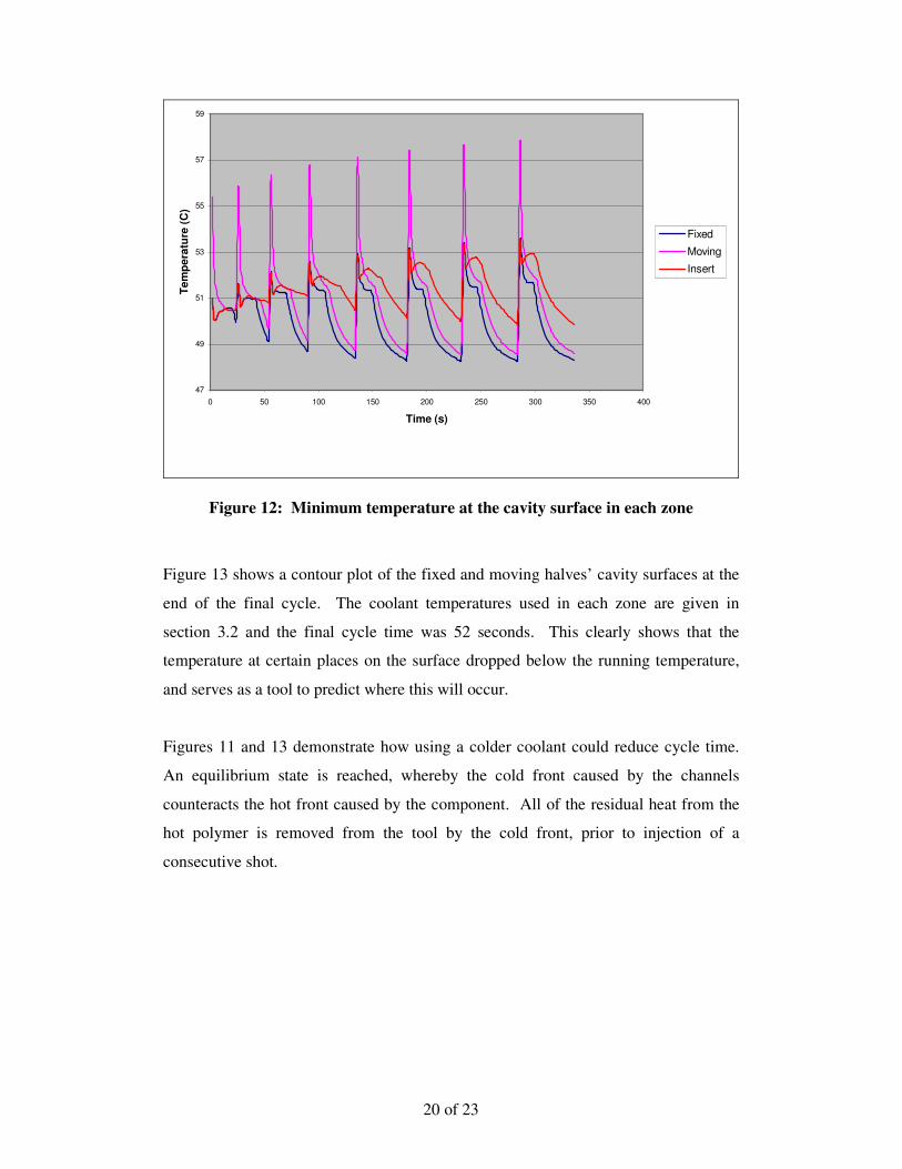
Figure 12 shows one of the significant advantages of using a numerical model to
analyse this system. An important factor that affects the properties of injection-
moulded components is the temperature at the surface of the cavity prior to the
injection of consecutive shots. It can be seen that the minimum computed
temperature at the surface of the cavity was found to be 48ºC in the fixed and moving
zones, prior to mould filling. This highlighted the need for some change to the
experimental setup. Increasing the coolant temperature in the two zones would
increase the minimum cavity temperature at the end of the cycle.
Figure 11: Temperature contour plot taken through the body of the tool using
the computational model
20 of 23
47
49
51
53
55
57
59
0 50 100 150 200 250 300 350 400
Time (s)
Tem
pera
ture
(C)
Fixed
Moving
Insert
Figure 12: Minimum temperature at the cavity surface in each zone
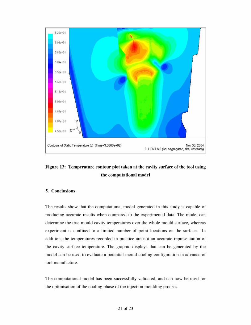
Figure 13 shows a contour plot of the fixed and moving halves’ cavity surfaces at the
end of the final cycle. The coolant temperatures used in each zone are given in
section 3.2 and the final cycle time was 52 seconds. This clearly shows that the
temperature at certain places on the surface dropped below the running temperature,
and serves as a tool to predict where this will occur.
Figures 11 and 13 demonstrate how using a colder coolant could reduce cycle time.
An equilibrium state is reached, whereby the cold front caused by the channels
counteracts the hot front caused by the component. All of the residual heat from the
hot polymer is removed from the tool by the cold front, prior to injection of a
consecutive shot.
21 of 23
Figure 13: Temperature contour plot taken at the cavity surface of the tool using
the computational model
5. Conclusions
The results show that the computational model generated in this study is capable of
producing accurate results when compared to the experimental data. The model can
determine the true mould cavity temperatures over the whole mould surface, whereas
experiment is confined to a limited number of point locations on the surface. In
addition, the temperatures recorded in practice are not an accurate representation of
the cavity surface temperature. The graphic displays that can be generated by the
model can be used to evaluate a potential mould cooling configuration in advance of
tool manufacture.
The computational model has been successfully validated, and can now be used for
the optimisation of the cooling phase of the injection moulding process.

22 of 23
Acknowledgments
The work described in this paper forms part of the Enhanced Polymer Processing
programme funded by the EPSRC, in collaboration with the University of Bradford
and Queen’s University Belfast. The authors would like to acknowledge the technical
support received from REPS Ltd and John Guest Ltd for the provision of the
experimental mould tool.
References
[1] B.A. McCalla, P.S. Allan, P.R. Hornsby, A.G. Smith, L.C Wrobel, A.L. Kelly
and P.D. Coates, Evaluation of pulsed cooling in injection mould tools, Polymer
Process Engineering 03, 52-71, Ed P.D. Coates, University of Bradford (2003)
[2] B.A. McCalla, P.S. Allan, P.R. Hornsby, Evaluation of heat management in
injection mould tools, Plastics, Rubber and Composites: Macromolecular
Engineering, 36, 26-33 (2007)
[3] B. Nardin, K. Kuzman, Z. Kampus, Injection moulding simulation results as an
input to the injection moulding process, Journal of Materials Processing
Technology 130, 310-314 (2002)
[4] S.W. Kim, L.S. Turng, Developments of three-dimensional computer-aided
engineering simulation for injection moulding, Modelling and Simulation in
Materials Science and Engineering 12, S151-S173 (2004)
[5] L. Sridhar, K. A. Narh, The effect of temperature dependent thermal properties
on process parameter prediction in injection moulding, International
Communications in Heat and Mass Transfer 27, 325-332 (2000)
[6] R. E. Promotion Services Ltd. (REPS), Temperature sensing probes,
[http://fp.repsuk.plus.com/products/probes.htm] (accessed 8/10/03)
[7] J. F. Stevenson, Innovation in Polymer Processing – Moulding, Hanser &
Gardener Publications Inc., pp. 425 – 430 (1996)
[8] Fluent 6.0 User Guide, Fluent Inc. (2003)
[9] Engineering.com, Typical values of convection heat transfer coefficient,

23 of 23
[http://www.engineering.com/content/ContentDisplay?contentId=41005014]
(accessed 17/03/2004)