A complexity score derived from principal components...

Physica A 301 (2001) 567–588www.elsevier.com/locate/physa

A complexity score derived from principalcomponents analysis of nonlinear order measuresAlessandro Giuliania , Mauro Colafranceschia , Charles L. Webber Jr.b ,

Joseph P. Zbilutc;∗aTCE Laboratory, Istituto Superiore di Sanit�a, V.le Regina Elena 299, Rome 00161, Italy

bDepartment of Physiology, Stritch School of Medicine, Loyola University Chicago, 2160 S. First Ave.,Maywood, IL 60153, USA

cDepartment of Molecular Biophysics and Physiology, Rush University, 1653 W. Congress, Chicago,IL 60612, USA

Received 13 July 2001

Abstract

The generation of a global “complexity” score for numerical series was derived from a prin-cipal components analysis of a group of nonlinear measures of experimental as well simulatedseries. The concept of complexity was demonstrated to be independent from other descriptorsof ordered series such as the amount of variance, the departure from normality and the relativenonstationarity; and to be mainly related to the number of independent elements (or operations)needed to synthesize the series. The possibility of having a univocal ranking of complexity fordiverse series opens the way to a wider application of dynamical systems concepts in empiricalsciences. c© 2001 Elsevier Science B.V. All rights reserved.

PACS: 02.50.Sk; 05.45.+b; 07.05.Kf; 87.10.+b

Keywords: Complexity; Singular value decomposition; Recurrence quanti>cation;Lempel–Ziv information; Stochastic process; Determinism

1. Introduction

Over the last two decades, a signi>cant debate has developed regarding the de>nitionand use of the concept of complexity, inspired in some degree by interest in determin-istic chaos [1]. A direct link between chaos theory and the real world was suggested byanalysis of time series data in situations ranging from heart rate [2] and brain activity

∗ Corresponding author. Tel.: +1-312-942-6008; fax: +1-312-942-8711.E-mail address: [email protected] (J.P. Zbilut).

0378-4371/01/$ - see front matter c© 2001 Elsevier Science B.V. All rights reserved.PII: S 0378 -4371(01)00427 -7

568 A. Giuliani et al. / Physica A 301 (2001) 567–588

[3] to >nancial markets [4]. Con>dence in these assertions diminished when questionsarose regarding the validity of these statements given that true chaotic systems aretypically stationary. Furthermore, numerous questions arose regarding the algorithmsused for detection of chaotic systems, given the rigorous mathematical assumptionsattending them. Consequently, interest in deterministic chaos has decreased in signif-icance for biological (real) systems, but a diJerent, more realistic view of basicallystochastic systems has yet to emerge. Nevertheless, computational tools developed todetect chaos continue to be used [5] to study the behavior of real experimental systems,despite the fact that estimates of chaotic invariants based on short and noisy data havequestionable validity. On the other hand, the completion of the genome project and therise of the so-called “post genomic” era have emphasized the need for having reliableand eLcient techniques to study complex systems such as DNA microarrays, nucleicacids and protein sequences [6].The character of biological data places signi>cant demands upon data analysis tools

given that many biological series cannot provide long data sets (e.g., a protein sequenceonly very rarely reaches 500 amino acids), data stationarity (virtually no biological sys-tems can be considered as stationary) and theoretical assumptions (there are no reliablemathematical theories for biological systems if we exclude very peculiar phenomenasuch as prey=predator interactions or pharmacokinetics). Given these prerequisites, thereare still many methodologies (based on various de>nitions) available which provide aquantitative estimation of the complexity of a system. Our question is “Is it possible tosingle out a unitary meaning from the plethora of complexity de>nitions distinct fromcognate concepts such as variance, nonnormality, or intermittency?” If this is the case,we should be able to demonstrate a basic commonality between the diJerent algorithmsused for complexity estimation. This basic concordance would allow the experimenterto shift from one technique to the other, depending on the character of the experimentaldata, while maintaining invariant the basic meaning of the description.We approached the problem from an experimental viewpoint, taking for granted the

impossibility of de>ning a common theoretical background for the myriads of diJer-ent experimental situations in which time (or spatial as in the case of linear macro-molecules) series are investigated. We simply collected a large and heterogeneous setof experimental series together with simulated series of known and controlled mathe-matical characteristics in order to look for a common scaling of the entire set whendescribed by a collection of diJerent complexity indexes. This common scaling wasdemonstrated by the application of principal components analysis (PCA) 1 of the dataset having as statistical units the series and as variables the complexity measures (seebelow). This approach is common in empirical science and used in such diverse >eldsas organic chemistry [7] and population genetics [8].

1 We use both PCA and singular value decomposition (SVD) in this study, which are related but diJerent.See below; also: G.W. Stewart, SIAM Review 35 (1993) 551. In general we will refer to PCA in the caseof the statistical analysis of the matrix having as units (rows) the 198 series and as variables (columns)the 13 descriptors; the term SVD will be used for the analysis of the single series in order to derive thecumulative descriptors e1 and SVSen (see Material and Methods).

A. Giuliani et al. / Physica A 301 (2001) 567–588 569

The obtained scaling, in the form of a cumulative complexity score corresponding tothe >rst eigenvector of the data set having as statistical units the single series and asvariables the indexes summarizing the output of diJerent mathematical descriptions ofthe series, was consistent with the properties of the simulated series and ful>lled someknown properties of the investigated experimental series. This opens the possibilityto obtain a consistent and quantitative measure of the amount of complexity of anykind of numerical series. Moreover, the minor, but nevertheless statistically signi>cantcomponents extracted by PCA allowed for a quantitative appreciation to other aspects ofseries characterization such as departure from normality or intermittency. The proposedscaling was generated by relatively short series (300–1000 points) thus pointing to thewide applicability of complexity measures to virtually all research >elds.

2. Materials and methods

2.1. Series collection

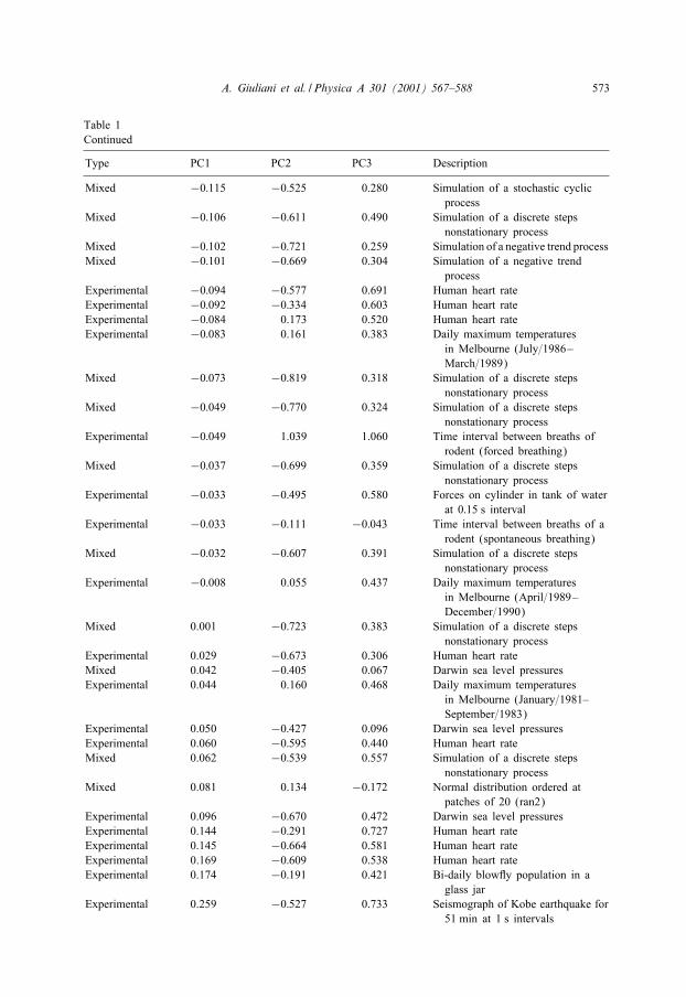
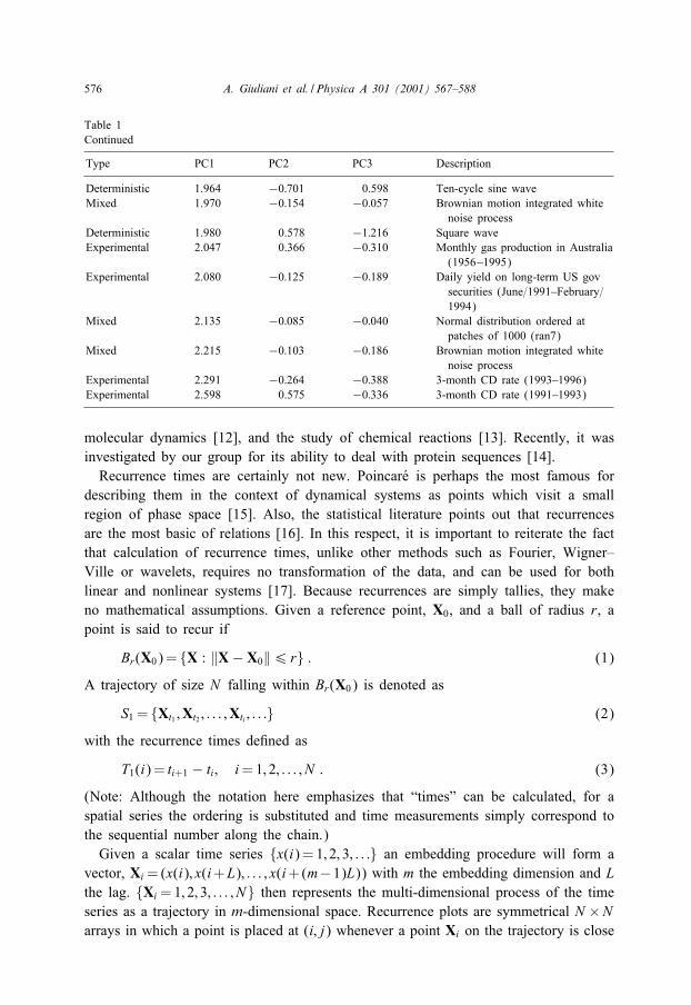
Almost 200 series were gathered and included four main types: random, mixed, de-terministic (which included chaotic examples) and experimental (Table 1). The lasttype refers to experimentally obtained series, while the >rst three types refer to thegeneration of simulated series used as “probes”. Random series are � digits and a num-ber of random number series coming from diJerent statistical distributions (Poisson,Gaussian, uniform). Series of a “mixed” type come from various blendings of uncorre-lated and correlated sources such as square waves corrupted by increasing amounts ofnoise (SNR#), Gaussian white noise linearly ordered along increasingly long segments(RAN#), or simply red=pink noise correlated by integration such as Brownian motion(Brownian#). “Deterministic” refers to a square wave and a sinusoid, and includes“chaotic” Henon, Lorenz and logistic series.

2.2. Complexity indexes

As stated in the introduction we limited ourselves to methods we could apply torelatively short series. The methods calling for the generation of an embedding matrix(recurrence quanti>cation, singular value decomposition; see below) were applied atembedding of 8 and a delay of 1. Recurrence quanti>cation adopted a radius equal tothe 20% of mean distances between the rows of the embedding matrix.

2.2.1. Embedding-based methods2.2.1.1. Recurrence quanti<cation. Recurrence quanti>cation analysis (RQA) is a rel-atively new nonlinear technique, originally suggested by Eckmann et al. [9] as a purelygraphical technique and then made quantitative by Zbilut and Webber [10]. The tech-nique has successfully applied in numerous >elds ranging from physiology [11] to


Table 1Components and descriptions

Type PC1 PC2 PC3 Description

Random −1:306 −0:022 −0:704 3001–3500 greek pi digitsRandom −1:303 0.031 −0:778 1–500 greek pi digitsExperimental −1:298 −0:051 −0:700 Radioactive decayRandom −1:297 −0:092 −0:723 2001–2500 greek pi digitsRandom −1:297 −0:037 −0:713 Simulation of a Gaussian stationary

processRandom −1:292 −0:096 −0:695 Simulation of a Gaussian stationary

processRandom −1:283 −0:057 −0:696 501–1000 greek pi digitsMixed −1:281 0.021 −0:613 Square wave plus Gaussian error at

SNR =0:25 (snr11)Random −1:275 −0:071 −0:692 2501–3000 greek pi digitsRandom −1:274 −0:031 −0:651 3501–4000 greek pi digitsRandom −1:270 −0:013 −0:620 Normal distributionRandom −1:268 −0:092 −0:642 Simulation of a Gaussian stationary

processRandom −1:265 −0:066 −0:740 1501–2000 greek pi digitsRandom −1:264 −0:057 −0:678 Simulation of a Gaussian stationary

processRandom −1:264 −0:076 −0:697 1001–1500 greek pi digitsRandom −1:259 −0:037 −0:634 Uniform distributionRandom −1:255 1.071 0.163 Poisson processMixed −1:251 −0:032 −0:612 Square wave plus Gaussian error at

SNR =0:35 (snr10)Random −1:232 −0:050 −0:674 Uniform distributionExperimental −1:231 −0:031 −0:454 Tree ringsMixed −1:203 −0:018 −0:477 Square wave plus Gaussian error at

SNR =0:45 (snr8)Mixed −1:202 −0:107 −0:497 Square wave plus Gaussian error at

SNR =0:40 (snr9)Experimental −1:201 −0:043 −0:392 Tree ringsMixed −1:171 0.060 −0:579 Square wave plus Gaussian error at

SNR =0:20 (snr12)Experimental −1:151 −0:169 −0:405 Tree ringsExperimental −1:145 −0:081 −0:204 Tree ringsExperimental −1:143 0.021 −0:244 Daily total female births in CaliforniaRandom −1:128 0.914 −0:034 Poisson processExperimental −1:103 −0:211 −0:969 Protein sequence (p73)Experimental −1:099 −0:137 −0:187 Tree ringsMixed −1:098 −0:188 −0:358 Square wave plus Gaussian error at

SNR =0:75 (snr6)Random −1:086 1.708 0.513 Poisson processExperimental −1:078 0.287 −0:620 Daily US exchange rates (1995–96)Experimental −1:076 −0:196 −0:924 Protein sequence (nphoc)Experimental −1:067 −0:190 −0:249 Tree ringsMixed −1:060 −0:047 −0:438 Square wave plus Gaussian error at

SNR =0:50 (snr7)Experimental −1:013 −0:388 −0:491 Tree ringsExperimental −1:008 −0:278 −0:990 Protein sequence (hnporc)Experimental −1:000 −0:359 −0:158 Tree ringsExperimental −0:999 −0:126 −1:053 Protein sequence (hnsen)


Table 1Continued


Experimental −0:991 −0:187 −0:876 Protein sequence (npsend)Experimental −0:970 −0:097 −0:948 Protein sequence (p63)Experimental −0:968 −0:143 −1:099 Protein sequence (hnsv41)Experimental −0:966 −0:294 −0:129 Tree ringsMixed −0:953 −0:177 −0:263 Square wave plus Gaussian error at

SNR =1 (snr5)Experimental −0:923 −0:360 −0:591 Protein sequence (npara1)Experimental −0:918 0.417 −0:588 Daily US exchange rates (1994–95)Experimental −0:894 −0:321 −0:136 Tree ringsExperimental −0:885 −0:046 −1:070 Protein sequence (fpho)Experimental −0:877 −0:199 −0:021 Tree ringsExperimental −0:855 −0:109 −1:085 Protein sequence (fsv5)Experimental −0:853 −0:111 −1:074 Protein sequence (fporc)Experimental −0:831 −0:217 −0:199 Square wave plus Gaussian error at

SNR =1:25 (snr4)Experimental −0:782 5.672 3.050 Daily rainfall in Melbourne

(April=1989–December=1990)Experimental −0:763 1.209 0.638 Time interval between breaths of a

rodent (spontaneous breathing)Experimental −0:731 0.074 −0:942 Protein sequence (p53)Experimental −0:728 −0:532 −0:031 Tree ringsExperimental −0:722 −0:209 0.314 Tree ringsExperimental −0:699 0.336 0.109 Time interval between breaths of a

rodent (forced breathing)Mixed −0:662 −0:461 −0:013 Square wave plus Gaussian error at

SNR =2:5 (snr3)Experimental −0:630 −0:348 0.105 Tree ringsExperimental −0:627 −0:608 0.410 Tree ringsExperimental −0:626 −0:577 0.150 Tree ringsExperimental −0:608 −0:347 −0:326 Monthly cars production in Australia

(1961–1995)Experimental −0:595 −0:284 0.285 Tree ringsExperimental −0:587 −0:622 0.205 Monthly values of the Southern

Oscillation Index during1950–1995

Experimental −0:577 3.652 1.320 Daily rainfall in Melbourne(January=1981–September=1983)

Experimental −0:559 0.474 0.544 Monthly Tows for Funder River(1919–1956)

Experimental −0:554 4.898 2.108 Daily rainfall in Melbourne(October=1983–June=1986)

Chaotic −0:505 0.632 −1:405 Logistic diJerence equation chaoticregion

Experimental −0:492 −0:198 −0:040 Seismograph of Kobe earthquake for51 min at 1 s intervals

Experimental −0:482 4.084 1.543 Daily rainfall in Melbourne(July=1986–March=1989)

Experimental −0:445 −0:309 0.032 Seismograph of Kobe earthquake for51 min at 1 s intervals

Mixed −0:437 0.003 −0:326 Normal distribution ordered atpatches of 10 (ran1)


Table 1Continued


Experimental −0:437 −0:746 0.273 Simulation of a negative trendprocess

Experimental −0:436 −0:297 0.019 Tree ringsExperimental −0:424 −0:352 0.184 Tree ringsExperimental −0:421 −0:176 −0:149 Seismograph of Kobe earthquake for

51 min at 1 s intervalsExperimental −0:406 1.600 1.147 EJective federal funds rate

(December=1995–October=1997)Experimental −0:348 −0:450 0.143 Tree ringsExperimental −0:341 −0:524 0.251 Oxygen isotope levelsExperimental −0:318 0.933 0.858 EJective federal funds rate

(June=1992–March=1994)Experimental −0:303 0.524 0.841 Monthly Tows for Mitta Mitta River

(1936–1968)Experimental −0:276 −0:471 0.312 Daily minimum temperatures

in Melbourne (July=1986–March=1989)

Experimental −0:274 −0:505 0.240 Daily minimum temperaturesin Melbourne (October=1983–June=1986)

Experimental −0:271 −0:261 0.253 Tree ringsMixed −0:270 −0:553 0.247 Simulation of a stochastic cyclic

processExperimental −0:246 −0:276 0.634 Tree ringsExperimental −0:242 −0:578 0.330 Daily minimum temperatures

in Melbourne (April=1989–December=1990)

Experimental −0:239 −1:734 2.477 Tree ringsExperimental −0:218 1.108 0.852 Monthly Tows for Colorado River

(1911–1972)Mixed −0:211 −0:552 0.380 Simulation of a positive trend processMixed −0:196 −0:562 0.279 Simulation of a stochastic cyclic

processExperimental −0:188 −0:412 0.401 Seismograph of Kobe earthquake for

51 min at 1 s intervalsMixed −0:157 −0:545 0.296 Simulation of a stochastic cyclic

processMixed −0:152 −0:510 0.370 Simulation of a positive trend

processMixed −0:146 −0:727 0.333 Simulation of a negative trend

processExperimental −0:142 −0:466 0.387 Daily minimum temperatures

in Melbourne (January=1981–September=1983)

Experimental −0:134 0.017 0.358 daily maximum temperaturesin Melbourne (October=1983–June=1986)

Mixed −0:127 −0:483 0.478 Simulation of a positive trendprocess

Mixed −0:127 −0:419 0.500 Simulation of a positive trendprocess


Table 1Continued


Mixed −0:115 −0:525 0.280 Simulation of a stochastic cyclicprocess

Mixed −0:106 −0:611 0.490 Simulation of a discrete stepsnonstationary process

Mixed −0:102 −0:721 0.259 Simulation of a negative trend processMixed −0:101 −0:669 0.304 Simulation of a negative trend

processExperimental −0:094 −0:577 0.691 Human heart rateExperimental −0:092 −0:334 0.603 Human heart rateExperimental −0:084 0.173 0.520 Human heart rateExperimental −0:083 0.161 0.383 Daily maximum temperatures

in Melbourne (July=1986–March=1989)



Experimental −0:049 1.039 1.060 Time interval between breaths ofrodent (forced breathing)


Experimental −0:033 −0:495 0.580 Forces on cylinder in tank of waterat 0:15 s interval

Experimental −0:033 −0:111 −0:043 Time interval between breaths of arodent (spontaneous breathing)


Experimental −0:008 0.055 0.437 Daily maximum temperaturesin Melbourne (April=1989–December=1990)

Mixed 0.001 −0:723 0.383 Simulation of a discrete stepsnonstationary process

Experimental 0.029 −0:673 0.306 Human heart rateMixed 0.042 −0:405 0.067 Darwin sea level pressuresExperimental 0.044 0.160 0.468 Daily maximum temperatures

in Melbourne (January=1981–September=1983)

Experimental 0.050 −0:427 0.096 Darwin sea level pressuresExperimental 0.060 −0:595 0.440 Human heart rateMixed 0.062 −0:539 0.557 Simulation of a discrete steps

nonstationary processMixed 0.081 0.134 −0:172 Normal distribution ordered at

patches of 20 (ran2)Experimental 0.096 −0:670 0.472 Darwin sea level pressuresExperimental 0.144 −0:291 0.727 Human heart rateExperimental 0.145 −0:664 0.581 Human heart rateExperimental 0.169 −0:609 0.538 Human heart rateExperimental 0.174 −0:191 0.421 Bi-daily blowTy population in a

glass jarExperimental 0.259 −0:527 0.733 Seismograph of Kobe earthquake for

51 min at 1 s intervals


Table 1Continued


Experimental 0.269 −0:861 −0:123 Monthly mean thickness ozonecolumns (Dobson units)(1791–1926)

Experimental 0.306 −0:277 0.114 Monthly beer production inAustralia (1956–1995)

Experimental 0.336 −0:275 0.718 Human heart rateExperimental 0.339 −0:314 0.671 Human heart rateExperimental 0.342 −0:419 0.523 Seismograph of Kobe earthquake for

51 min at 1 s intervalsExperimental 0.348 −0:335 0.767 Human heart rateExperimental 0.371 −0:604 0.219 Monthly bricks production in

Australia (1956–1995)Experimental 0.379 5.876 4.473 EJective federal funds rate

(July=1986–December=1987)Experimental 0.393 −0:537 0.465 Monthly sulphuric acid production

in Australia (1956–1994)Mixed 0.397 −0:693 0.509 Square wave plus Gaussian error at

SNR =5 (snr2)Chaotic 0.417 0.114 −0:853 Logistic mapExperimental 0.446 1.375 1.398 EJective federal funds rate

(January=1985–June=1986)Mixed 0.447 −0:859 0.711 Ten-cycle sine wave added uniform

white noiseExperimental 0.448 −0:075 0.266 Monthly chocolate production in

Australia (1957–1995)Experimental 0.535 0.597 0.139 Time interval between breaths of a

rodent (forced breathing)Experimental 0.614 −0:620 0.160 Monthly blooms and slabs produc-

tion in Australia (1956–1995)Experimental 0.621 −0:591 0.160 Monthly rawsteel production in

Australia (1956–1993)Experimental 0.670 −0:757 0.865 Protein structure (cpp3)Experimental 0.675 −0:387 0.187 EJective federal funds rate

(October=1997–July=1999)Mixed 0.712 0.157 −0:152 Normal distribution ordered at

patches of 50Experimental 0.748 −0:264 0.057 Time interval between breaths of a

rodent (forced breathing)Experimental 0.764 0.110 0.771 Monthly means of daily relative

sunspot numbers (1749–1832)Experimental 0.769 −0:786 0.841 Protein structure (phh1)Experimental 0.785 0.076 0.676 Monthly means of daily relative

sunspot numbers (1833–1915)Experimental 0.791 −0:064 0.797 Monthly means of daily relative

sunspot numbers (1916–1977)Experimental 0.844 −0:575 0.190 Monthly iron production in Australia

(1956–1995)Chaotic 0.860 −0:485 0.610 Lorenz attractorChaotic 0.886 −0:429 0.624 Lorenz attractorExperimental 0.913 −0:746 0.835 Protein structure (phh2)Mixed 0.924 −0:289 0.063 Square wave plus Gaussian error at

SNR =10 (snr1)


Table 1Continued


Experimental 1.015 0.056 0.537 Wheat prices (1264–1996)Mixed 1.083 0.095 −0:074 Normal distribution ordered at

patches of 100 (ran4)Experimental 1.090 −0:328 0.169 Daily brightness of a variable star

on 600 successive midnightsExperimental 1.257 −0:494 0.558 Daily yield on long-term US

government securities (October=1988–June=1991)

Experimental 1.277 0.017 0.152 EJective federal funds rate(November=1988–August=1990)

Mixed 1.320 0.070 −0:063 Normal distribution ordered atpatches of 200 (ran5)

Experimental 1.340 0.087 0.052 EJective federal funds rate(August=1990–May=1992)

Experimental 1.368 −0:527 0.551 Protein structure (cpp1)Experimental 1.371 −0:232 −0:320 EJective federal funds rate

(March=1994–December=1995)Experimental 1.407 −0:584 0.405 Protein structure (phh3)Experimental 1.408 −0:571 0.244 Protein structure (cpp2)Experimental 1.484 −0:406 0.176 10-year Treasury constant maturity

rateChaotic 1.495 1.672 −3:229 Henon variable for 16-point periodic

processChaotic 1.495 1.672 −3:229 Henon variable for 16-point periodic

processExperimental 1.520 −0:296 0.278 3-month CD rate (1996–1999)Experimental 1.570 −0:083 −0:167 EJective federal funds rate

(July=1999–April=2001)Chaotic 1.573 1.670 −3:261 Logistic diJerence equation period-4

regionExperimental 1.635 −0:342 0.240 Daily yield on long-term US

gov securities (March=1986–October=1988)

Experimental 1.646 3.333 −5:810 2 digit Toating point valuesExperimental 1.648 3.329 −5:798 2 digit Toating point valuesMixed 1.687 0.055 −0:138 Normal distribution ordered at

patches of 500 (ran6)Mixed 1.697 −0:156 0.096 Brownian motion integrated white

noise processMixed 1.700 −0:413 −0:160 Brownian motion integrated white

noise processExperimental 1.709 −0:296 0.025 Daily yield on long-term US

gov securities (February=1994–October=1996)

Experimental 1.853 0.058 −0:256 Monthly electricity production inAustralia (1956–1995)

Experimental 1.865 −0:149 0.045 3-month CD rate (1999–2001)Experimental 1.915 −0:427 0.421 Tracheal pressure trace from a

spontaneously breathing rodentExperimental 1.936 −0:324 0.381 Tracheal pressure trace from a

spontaneously breathingrodent


Table 1Continued


Deterministic 1.964 −0:701 0.598 Ten-cycle sine waveMixed 1.970 −0:154 −0:057 Brownian motion integrated white

noise processDeterministic 1.980 0.578 −1:216 Square waveExperimental 2.047 0.366 −0:310 Monthly gas production in Australia

(1956–1995)Experimental 2.080 −0:125 −0:189 Daily yield on long-term US gov

securities (June=1991–February=1994)

Mixed 2.135 −0:085 −0:040 Normal distribution ordered atpatches of 1000 (ran7)

Mixed 2.215 −0:103 −0:186 Brownian motion integrated whitenoise process

Experimental 2.291 −0:264 −0:388 3-month CD rate (1993–1996)Experimental 2.598 0.575 −0:336 3-month CD rate (1991–1993)

molecular dynamics [12], and the study of chemical reactions [13]. Recently, it wasinvestigated by our group for its ability to deal with protein sequences [14].Recurrence times are certainly not new. PoincarUe is perhaps the most famous for

describing them in the context of dynamical systems as points which visit a smallregion of phase space [15]. Also, the statistical literature points out that recurrencesare the most basic of relations [16]. In this respect, it is important to reiterate the factthat calculation of recurrence times, unlike other methods such as Fourier, Wigner–Ville or wavelets, requires no transformation of the data, and can be used for bothlinear and nonlinear systems [17]. Because recurrences are simply tallies, they makeno mathematical assumptions. Given a reference point, X0, and a ball of radius r, apoint is said to recur if

Br(X0)= {X : ‖X − X0‖6 r} : (1)

A trajectory of size N falling within Br(X0) is denoted as

S1 = {Xt1 ;Xt2 ; : : : ;Xti ; : : :} (2)

with the recurrence times de>ned as

T1(i)= ti+1 − ti; i=1; 2; : : : ; N : (3)

(Note: Although the notation here emphasizes that “times” can be calculated, for aspatial series the ordering is substituted and time measurements simply correspond tothe sequential number along the chain.)Given a scalar time series {x(i)= 1; 2; 3; : : :} an embedding procedure will form a

vector, Xi =(x(i); x(i+L); : : : ; x(i+(m−1)L)) with m the embedding dimension and Lthe lag. {Xi =1; 2; 3; : : : ; N} then represents the multi-dimensional process of the timeseries as a trajectory in m-dimensional space. Recurrence plots are symmetrical N ×Narrays in which a point is placed at (i; j) whenever a point Xi on the trajectory is close


to another point Xj. The closeness between Xi and Xj is expressed by calculating theEuclidian distance between these two normed vectors, i.e., by subtracting one fromthe other: ‖Xi − Xj‖6 r where r is a >xed radius. If the distance falls within thisradius, the two vectors are considered to be recurrent, and graphically this can beindicated by a dot. An important feature of such matrixes is the existence of shortline segments parallel to the main diagonal, which correspond to sequences (i; j); (i+1; j+ 1); : : : ; (i+ k; j+ k) such that the piece of X(j); X(j+ 1); : : : ;X(j+ k), is closeto X(i); X(i + 1); : : : ;X(i + k) in series which are deterministic. The absence of suchpatterns suggest randomness [9].Thus, recurrence plots simply correspond to the distance matrix between the diJerent

epochs (rows of the embedding matrix) >ltered, by the action of the radius, to abinary 0=1 matrix having a 1 (dot) for distances falling below the radius and a 0 fordistances greater than radius. Distance matrices have been shown to convey all relevantinformation for the global reconstruction of a system and thus represent exhaustiverepresentations of studied phenomena [18].Because graphical representations may be diLcult to evaluate, Zbilut and Webber

[10] developed several strategies to quantify features of such plots originally pointedout by Eckmann et al. [9]. Hence, the quanti>cation of recurrences leads to the gen-eration of >ve variables including: REC—percent of plot >lled with recurrent points;DET—percent of recurrent points forming diagonal lines, with a minimum of twoadjacent points; ENT—Shannon information entropy of the line length distribution;MAXLN—length of longest line segment (the reciprocal of which is an approxima-tion of the largest positive Liapunov exponent and is a measure of system divergence,Ref. [19]); and TREND—a measure of the paling of recurrent points away from thecentral diagonal. These >ve recurrence variables quantify the deterministic structureand complexity of the plot: REC quanti>es the amount of cyclic behavior; DET theamount of determinism through the counting of “sojourn points” [20]; ENT the richnessof deterministic structuring (and in this sense, has a somewhat opposite meaning withrespect to classical notion of entropy); MAXLN scales with the maximum Liapunovexponent; while TREND is essentially a measure of nonstationarity. These >ve indexesgive a summary of the autocorrelation structure of the series and were demonstrated,by means of a psychometric approach [21], to correlate with the visual impression thata group of unbiased observers derive from the inspection of an ensemble of recurrenceplots.

2.2.1.2. Singular value decomposition. Singular value decomposition (SVD) is awell-established method, and has had a long history in physical as well as in socialand biological sciences, and roughly corresponds to PCA. The term SVD is preferredto the term PCA in physical applications and, in general, when dealing with dynamicalphenomena. As in PCA, the aim of SVD is to project an originally multidimensionalphenomenon on a reduced set of new axes, each orthogonal to each other, representingthe basic modes explaining the analyzed data set. When applied to a time (or spatial)series, that is originally monodimensional. SVD necessitates that the original series be


represented on a multidimensional space by the agency of the embedding procedure.This “expansion” of the original monodimensional series onto a multidimensional sup-port allows for the autocorrelation structures present in the series to be appreciated asclassical between variables statistical correlations [22].The embedding matrix (EM) can be thought of as a multivariate matrix having

the series equal to the embedding dimension as statistical units (rows) and the wholesequence lagged by subsequent delays as variables (columns). Thus the EM can beconsidered as an M;N matrix, with M the number of elements subtracted from theembedding dimension (the last elements are eliminated by the shifting of the seriesdue to the embedding procedure) and the embedding dimension.A basic theorem in linear algebra states that each M ;N matrix X can be expressed

as

X =USV T ; (4)

where the matrices U and V are of dimensions M;K and N; K , respectively, and ful>llthe relations UTU =V TV =1. The K; K matrix S (typically the covariance matrix)is diagonal and has its diagonal elements (singular values) arranged in descendingorder s1¿s2¿s3 · · ·¿sk ¿ 0. In intuitive terms this means that the original datacan be projected onto a new set of coordinates US (principal component scores oreigenfunctions) such that no original information is lost. Given that each element ofX is immediately reconstructable by the equation

Xij =∑

UikSkVjk ; k =1; : : : ; N : (5)

The new coordinates are orthogonal by construction (i.e., statistically independent),each representing an independent aspect of the data set.PCA (and equivalently SVD) has an optimal property that made this method one of

the most widespread modeling techniques in diverse science >elds: with the expansiontruncated to A terms (with A¡N ) one obtains the summation

Xij =∑

UikSkVjk + Eij; k =1; : : : ; A ; (6)

where the squared error term, E2ij, is a minimum. What diJerentiates (5) from (6) is the

presence of the error term Eij and the limitation of the summation to a lower numberof coordinates with respect to the original data set. The fact that the error term is aminimum implies that the projection of the original data on the new component spacespanned by a smaller number of dimensions (A¡N ) is optimal in a least-squaressense. This implies that the meaningful (signal-like) part of the information is retainedby the >rst principal components, while discarding the noise in the noise Toor.In other words, the most correlated portion of information is retained by the >rst

components, while all the singularities are discarded in the minor components. The factthat more complex systems are characterized by a spread of energy away from the >rstsingular values can be quanti>ed by the index:

SVSen=−∑

si log si; i=1; : : : ; N : (7)


This is simply the Shannon formula applied to the distribution of normalized eigenval-ues, where si are the normalized singular values [23]. In our analysis we selected bothSVSen and the >rst eigenvalue score e1 as complexity descriptors.

2.2.2. Nonembedding related methodsThe methods described above rely on the necessity of a priori setting of measurement

parameters such as embedding dimension and, in the case of RQA, the value of adistance threshold (radius). This could be questionable (we demonstrate that a simple“common sense” choice of these parameters, common to all the analyzed series does notdisturb the obtained results below), so we decided to complement the above techniqueswith other complexity measures not depending on parameter setting.The nonembedding related measures we adopted for this work were: Lempel–Ziv

complexity (LZ), Pearson’s correlation coeLcient (Pearson), coeLcient of variation(CV), skewness (Skew), kurtosis (Kurt) and Hurst exponent (Hurst).The most widely used descriptor for algorithmic complexity, for its ease in imple-

mentation, and wide applicability, is the so-called Lempel–Ziv information content (LZ)[24]. LZ transforms the representation of a numerical sequence into a binary format,substituting 1 for the higher-than-median values and 0 otherwise. This binary sequenceis then analyzed trying to generate any subsequent con>guration of 1’s and 0’s from theprevious one using just two operators: copy and insert acting on the initial sequence.Starting from an initial random sequence, the procedure progressively reconstructs anypre-de>ned series: the number of instructions (copy plus insert operations) needed toproduce the series, normalized by the number of instructions needed to generate thecorresponding random sequence, constitutes the LZ index.Pearson’s correlation corresponds to the well-known statistical formula:

r=Cov(XY )=√(Var(x)Var(y)) ; (8)

where X and Y are adjacent values in the series Cov=Covariance and Var is thevariance. This is a measure of how strongly each data point correlates with itsimmediate predecessor, and points to a special kind of deterministic structure.CV is simply the ratio of standard deviation to mean, and measures the statistical

variability of the studied series independent of their scale.Skewness is expressed as

Skew=1N

N∑i=1

[(xi − Yx)

$

]3(9)

with N = number of points, xi =actual value of ith observation, and $; the standarddeviation. The related kurtosis is expressed as diJerence between actual kurtosis andthe kurtosis value of a Gaussian distribution:

Kurt=

{1N

N∑i=1

[(xi − Yx)

$

]4}− 3 : (10)


Skewness measures the departure from symmetry around the mean value of the prob-ability density function, while kurtosis measures the relative sharpness of the modalvalue with respect to the Gaussian distribution.The last descriptor we used is the Hurst exponent (Hurst) corresponding to the

slope of the curve linking mean-square displacement from initial position and time,using each point in the time series as an initial condition [25]. The exponent isde>ned as

H = log(R=S)=log(T ) ; (11)

where T is the duration of the sample of data, and R=S is the range of the cumulativedeviations from the mean divided by the standard deviation. The Hurst exponent is ameasure of the relative persistent=intermittent character of the series: values around 0.5point to Brownian motion-like behavior (coloured noise), exponents greater than 0.5indicate persistence (past trends persist into the future), whereas exponents less than0.5 indicate antipersistence (past trends tend to reverse into the future).

2.3. Strategy of analysis

The 13 quantitative descriptors presented above were computed for all the 198selected series to obtain a multivariate data matrix (DM) with 198 units and 13 vari-ables constituting the starting material of our analysis. The DM was submitted to a PCAto extract the relevant factors (principal components) shaping the diJerences betweenthe 198 series. The components are independent from each other by construction, andrepresent the independent concepts explaining the observed results [26]. The extractedcomponents were interpreted by means of inspection of component loadings, and corre-lation coeLcients between original descriptors and the components. The >rst component(corresponding to global complexity) was examined for consistency between obtainedcomplexity rankings and simulated series as well as with known peculiarities of someexperimental series. The fact that principal components were extracted in standardizedunits, having a zero mean and a unit standard deviation, helps in the interpretation ofthe obtained scaling.

3. Results

Fig. 1 reports the eigenvalues distribution at increasing component number: a simplevisual scree test [27] suggest two possible solutions for the number of signi>cantcomponents: a minimal three components solution, and a maximal >ve componentssolution. Higher order components are attributable to the “noise Toor” which, in thisparticular case, corresponds to the algorithmic minor subteleties of the methods notattributable to any particular feature of the studied series. The >rst component explains48% of the total variance, while the other “signal” components explain 15%, 13%, 8%and 6% of the total variance.


0 5 10 15

COMPONENT

0

1

2

3

4

5

6

7

EIG

EN

VA

LU

E

Fig. 1. Scree plot of PCs.

Table 2Component correlations

Variable PC1 PC2 PC3 PC4 PC5

Skew −0:031 0.783 0.531 −0:019 −0:002Kurt −0:110 0.815 0.498 −0:005 −0:023Pearson 0.541 −0:420 0.660 0.092 0.024LZ −0:949 0.023 −0:017 −0:030 −0:175Hurst 0.474 −0:413 0.578 −0:148 −0:125e1 0.921 −0:170 0.088 0.050 0.163REC 0.685 0.423 −0:506 −0:024 −0:010DET 0.875 0.224 0.064 0.040 0.172ENT 0.887 0.271 −0:180 0.058 0.141TREND −0:621 −0:027 −0:018 −0:117 0.727CV −0:119 0.011 −0:019 0.976 −0:001MAXLN 0.790 0.126 −0:306 −0:143 −0:236SVSen −0:960 0.131 −0:020 −0:033 −0:100

In addition to the complexity score (PC1), Table 1 also reports the second andthird components of the PCA scaling for nonlinear complexity descriptors (PC2 andPC3) pointing, respectively, to the departure from normality and relative continuous=intermittent character of the series. These were recognized as the two most importantdeterminants of series description other than the major complexity component.Table 2 reports the component loadings, i.e., the correlation coeLcients of the orig-

inal complexity descriptors with the extracted components. The >rst component (PC1)clearly corresponds to a global inverse complexity score, being very strongly relatedto LZ (r= − 0:949), e1 (r=0:921), SVSen (r= − 0:960); and signi>cantly corre-lated with the RQA variables, DET and ENT (r=0:875 and 0.889, respectively). It isworth noting that the complexity score is virtually independent from statistical (order


independent) properties of the probability distribution of the series (r= − 0:031 withSkew, r=− 0:110 and −0:119 with Kurt and CV, respectively).This result provides a clear-cut, completely data-driven, de>nition of complexity as

the number of order parameters (in the form of statistical correlations as in SVD orproduction rules as for LZ index) necessary to synthesize (reconstruct) the series. Inother words complexity takes the form of “number of degrees of freedom” of thedata. It is worth noting that there is no diJerence between embedding related andnonembedding related methods (the correlation coeLcient between LZ and SVSen isr=0:93): this means that, if we choose a suLciently high embedding dimension we aresure of not biasing our measures. In general, this suggests that the algorithmic notionof complexity is practically superimposable to the de>nition based on multivariate dataanalysis.The general complexity component is by far the most important order parameter

shaping the between series diJerences, whereas the other components point to minoraspects of the series that, independently from complexity, describe the studied phenom-ena. PC2 is a pure “probability distribution” factor and corresponds to the departurefrom normality. In fact it scales with Skew and Kurt (r=0:783 and 0.815, respec-tively) and has nothing to do with order-dependent descriptors. PC3 deals with therelative continuous=intermittent character of the series. In fact, the third component ispositively correlated with the Pearson coeLcient between adjacent values (r=0:660),Hurst exponent (r=0:578), and negatively correlated with REC (r= − 0:506). It isworth noting that higher order components tend to have lower values of loadings anda lower number of variables correlated with them with respect to higher order com-ponents for the obvious reason that they explain small percentages of the variance.On the other hand, a single descriptor could participate in more than one componentbecause its value depends upon more than one basic factor. For example, this is thecase for REC which is inTuenced by both “complexity at large” (r=0:685 with PC1)and “continuity=intermittence” (r= − 0:506 with PC3) or for Pearson (r=0:541 withPC1 and r=0:660 with PC3). In this respect is noticeable that TREND is correlated atr=−0:621 with PC1 and r=0:727 with PC5 suggesting the degree of “non-stationarity”of the series independent of other features (pure nonstationarity). Normalized variance(CV) has a PC for its own (PC4) with which it is highly correlated (r=0:976). Thisimplies that statistical (order independent) variability is a concept completely distinctfrom complexity.Having described the extracted components from the point of view of the original

variables (descriptors of the series), we next consider a description of the componentspace from the point of view of the statistical units, i.e., by the consideration of therelative locations of the studied series in component space. Figs. 2 and 3 report thePC1–PC2 and PC1–PC3 bidimensional spaces: the points correspond to the studiedseries, with some notable series labeled. At >rst it is important to note how only PC1constitutes a continuous ranking of the series, the other factors are mainly driven bysome peculiar (outlier) series such as the Melbourne rainfall series characterized byboth a big departure from normality (high values of PC2) and a marked “persistency”


-2 -1 0 1 2 3

PC1

-2

-1

0

1

2

3

4

5

6

PC

2

Fed. Funds

NumericalAccuracy

Henon

Fed.Credits

Tree Ring (India)

Poisson

RadioactiveDecay

MelbourneRainfall

π

Fig. 2. PC1–PC2 space.

-2 -1 0 1 2 3

PC1

-10

-5

0

5

PC

3

Fed.

Credits

Tree Ring

SquareWave

Logistic

Henon

NumericalAccuracy

MelbourneRainfall

Fig. 3. PC1–PC3 space.

both due to the presence of very characterized “rain days clusters”, as well as the gen-eral unpredictability of the series (the points are shifted toward the “high complexity”end of PC1). On the other hand, “intermittency” (low values of PC3) is a well knownfeature of both the logistic and Henon series, and helps to explain the peculiar positionof the numerical accuracy series.The breadth of the global complexity axis ranging from pure randomness (radioac-

tive decay) to very deterministic series (square wave) is evident together with theplacement of deterministic chaos at the “low complexity” pole of the axis. This loca-tion of deterministic chaos at the low complexity pole is reminiscent of many of the


methods that were designed to separate deterministic chaos from pure randomness. Itis equally evident that experimental series are generally similar to the “mixed” typeseries. This feature suggests a direct use of the component space to give a “coarsegrain” characterization to experimental series for which a reliable physical model isnot available: each experimental series can be compared with to a similar simulatedseries, which then suggest a “>rst hypothesis” for the right model. It is important tostress the fact that, since PCs are linear combinations of the original variables, it issimple to compute by a multiple linear regression equation, the principal componentscore relative to a nonanalyzed series, thus automatically scaling this new series withrespect to the others. This use of PCA is very common in various applicative >elds, es-pecially in medicinal chemistry where “control component charts” are used to allocatenewly synthesized organic molecules [28].In the present application we built some standard samples to calibrate our >ndings

for order (and alternatively disorder) to check if the global complexity score ranksthese series correctly. The two series of standards we used were the RAN# and SNR#series. The RAN# series were generated from a 1000 points simulation from a Gaussiandistribution with elements organized in an increasing linear order along patches ofdiJerent length [29]: thus RAN1 was created by ordering the series 10×10; i.e., puttingthe >rst ten numbers in increasing order, then putting the second ten in increasing orderand so forth. RAN2 was created by patches of 20, until 1000 points were obtained.The SNR# series were generated by a square wave to which were added increasingamounts of Gaussian noise, starting from a signal-to-noise ratio of 10 (SNR1 series)and ending with a signal-to-noise ratio of 0.2 (SNR12 series) (Fig. 4). Both the “orderparameters” structuring the two families of time series; i.e., the patch length (Fig. 5a)and the signal-to-noise ratio (SNR) (Fig. 5b) were unequivocally recognized by theglobal complexity score.Having tested the system as for its consistency with simulated sets, we investigated

the coherence of the synthetic global score with what is known about some experimentalseries. The most paradigmatic case is that of protein sequences and structures: wehave in our data set twelve diJerent protein sequences coded in terms of the relativehydrophobicity of their amino acid residues [30], namely: p73, nphoc, hnporc, hnsen,npsend, p63, hnsv41, npara, fpho, fsv5, fporc, and p53.The protein sequences expressed in terms of the hydrophobicity score of their amino

acid residues are placed by our general scaling very close to pure randomness, butclearly (even if slightly) separated from pure randomness, going from a value of −1:10to a value of −0:74 while simulated random series go from −1:31 to −1:10 along PC1(t-test value= 10:3; p¡ 0:00001) (Fig. 6). The slight deviation of protein hydropho-bicity ordering is a well-known characteristic of protein primary structures [31] clearlydemonstrated by the analysis. Moreover, the p53 sequence, which is known to have aparticularly deterministic structuring of hydrophobicity due to its very peculiar biologi-cal role, was correctly placed at the “deterministic” end of protein sequence distribution.This means the obtained scaling, despite the huge heterogeneity of the studied system,allows for relatively >ne measurements.


0 100 200 300 400 500 600 700 800 900 1000-5

0

5

0 100 200 300 400 500 600 700 800 900 1000-5

0

5

0 100 200 300 400 500 600 700 800 900 1000-5

0

5

0 100 200 300 400 500 600 700 800 900 10000

20

40

0 100 200 300 400 500 600 700 800 900 1000-100

0

100

0 100 200 300 400 500 600 700 800 900 1000-200

0

200

ran1

ran3

ran5

snr1

snr7

snr12

Fig. 4. “Standard signals.”

0.5 1.0 1.5 2.0 2.5 3.0 3.5

LOGPATCH

-2

-1

0

1

2

3

PC

1

r =

0.992

0 2 4 6 8 10 12

SNR

-2

-1

0

1

PC

1

r =

0.972

(a) (b)

Fig. 5. (a,b) Correlation of “order parameters” of standard signals with PC1.

On the other hand we have inserted in our data set six series generated by thethree-dimensional structures of two diJerent proteins (cpp and phh): these series corre-spond to the x; y and z spatial coordinates of the constituent amino acids (expressed interms of their *-carbons). Obviously, given that adjacent amino acids are constrained


Protein Random

SERIES

-1.40

-1.25

-1.10

-0.95

-0.80

PC

1

Fig. 6. Comparison of protein sequences with random series.

by the presence of a chemical bond between them, these series have a strong inter-nal correlation like any polymer series [32], and, in fact, they are shifted toward thedeterministic end of the spectrum (PC1 ranging between 0.67 and 1.41).Another important aspect of these results points to the fact that experimental and

naturalistic data is strongly inTuenced by the methods by which this data is collected.For example, economic data may be averaged as well as linked to the agency of humaninstitutions. This is strongly suggested by the placement of federal funds and creditswhich may be intermittent, processed, and=or skewed (reTecting also the possibility offederal policies). A similar scenario may obtain with tree ring data which is stronglyinTuenced by prevailing weather patterns, which may be cyclic (Figs. 2 and 3). Lab-oratory data is often “>ltered” either purposefully or by limitations of instrumentation(e.g., band-width limitations). Thus these results suggest a caution for data which maybe “censored” either naturally or unknowingly. It is also interesting to note that someprocesses such as the heartbeat are situated in the middle between randomness anddeterminism, contrary to the advocates for cardiac chaos. An alternative view has beento consider the heartbeat as an alternation between deterministic and stochastic pro-cesses and appears to have some support here. This alternating stochastic=deterministicdynamic has been termed “terminal dynamics”, and may be a new paradigm for manynatural phenomena [33].

4. Conclusions

The notion of “amount of complexity” emerging from these results resembles theclassical mechanical notion of complexity as the number of degrees of freedom suchthat a system with N particles has 3N − r degrees of freedom, r being the number of


DetExp M

ix

Random

GROUP

-2

-1

0

1

2

PC

1

Fig. 7. PC1 means (+=− SD) of main groups of studied series.

links (in our case correlations) linking the N elements. Normalizing for N the complex-ity remains inversely proportional to r; i.e., the number (and strength) of correlationspresent in the data. This simple reasoning uni>es the “equation-like” representation(like SVD wherein signal components can be directly equated with independent equa-tions of motion) and the “algorithmic complexity” view (where “symbolic rules” playthe role of equations). Increasing the number of links between the elements reducesthe number of equations necessary to describe the system.What appears to be important in this analysis is information, but not information in

the usual order-independent sense, rather, in the order-dependent sense. (Recall that agiven degree of freedom can have varying amounts of information capacity.) The >rstPC clearly emphasizes the role of information, algorithmically or through recurrenceas an order-dependent process. In this respect, this >nding supports observations thatordered information is a cornerstone of the physical sciences [34] with maximum com-plexity at one end, and determinism at the other [35]. Clearly, this bears a comfortingintuitionally real aspect making complexity relatively “simple”. Indeed, an inspectionof the categories relative to their complexity scores are signi>cantly separated fromeach other in this aspect; whereas, experimental and mixed data are clearly situated inthe middle (Fig. 7).A >nal remark is the demonstration that an unambiguous and self-consistent mea-

sure of complexity can be obtained for virtually any time (or spatial) series well in-side the data lengths typically attainable by experimentation. Moreover, the possibilityof applying eigenvalue methods directly to correlation matrixes (e.g., reticular sys-tems or directed graphs) enlarge the reach of the proposed method well beyond timeseries.


References

[1] G. Nicolis, I. Prigogine, Exploring Complexity, W.H. Freeman, New York, 1989.[2] J.E. Skinner, A.L. Goldberger, G. Mayer-Kress, R.E. Ideker, Biotechnology 8 (1990) 1018.[3] W.J. Freeman, Int. J. Bifurcation Chaos 2 (1992) 451.[4] D.A. Hsieh, J. Finance 46 (1991) 1839.[5] T. Schreiber, Phys. Reports 308 (1999) 1.[6] N.S. Holter, M. Mitra, A. Maritan, M. Cieplak, J. Banavar, N. FedoroJ, Proc. Natl. Acad. Sci. USA

97 (2000) 8409.[7] T.I. Oprea, J. Gottfries, J. Comb. Chem. 3 (2001) 157.[8] L.L. Cavalli-Sforza, P. Menozzi, A. Piazza, Science 259 (1993) 639.[9] J.-P. Eckmann, S.O. Kamphorst, D. Ruelle, Europhys. Lett. 4 (1987) 973.[10] J.P. Zbilut, C.L. Webber Jr., Phys. Lett. A 171 (1992) 199.[11] R. Balocchi, A. DiGarbo, C. Michelassi, S. Chillemi, M. Varanini, M. Barbi, J.M. Legramante,

G. Raimondi, J.P. Zbilut, Method Inform. Med. 39 (2000) 157.[12] C. Manetti, M.-A. Ceruso, A. Giuliani, C.L. Webber Jr., J.P. Zbilut, Phys. Rev. E 59 (1999) 992.[13] J.P. Zbilut, A. Giuliani, C.L. Webber Jr., A. Colosimo, Prot. Eng. 11 (1998) 87.[14] A. Giuliani, R. Benigni, P. Sirabella, J.P. Zbilut, A. Colosimo, Biophys. J. 78 (2000) 136.[15] M. Kac, Probability and Related Topics in Physical Sciences, Intersciences, New York, 1959.[16] W. Feller, An Introduction to Probability Theory and its Applications, Vol. 1, Wiley, New York, 1968.[17] C.L. Webber Jr., J.P. Zbilut, J. Appl. Physiol. 76 (1994) 965.[18] C.R. Rao, S. Suryawanshi, Proc. Natl. Acad. Sci. USA 93 (1996) 12 132.[19] L.L. Trulla, A. Giuliani, J.P. Zbilut, C.L. Webber Jr., Phys. Lett. A 223 (1996) 225.[20] J. Gao, H. Cai, Phys. Lett. A 270 (2000) 75.[21] A. Giuliani, P. Sirabella, R. Benigni, A. Colosimo, Prot. Eng. 13 (2000) 671.[22] D.S. Broomhead, G.P. King, Physica D 20 (1986) 217.[23] A.M. Sabatini, Med. Biol. Eng. Comput. 38 (2000) 617.[24] F. Kaspar, K.G. Schuster, Phys. Rev. A 36 (1987) 842.[25] J. Feder, Fractals, Plenum, New York, 1988.[26] L. Lebart, A. Morineau, K.M. Warwick, Multivariate Descriptive Statistical Analysis, Wiley,

New York, 1984.[27] R.B. Cattell, Multiv. Behav. Res. 1 (1966) 245.[28] T.I. Oprea, J. Gottfries, J. Comb. Chem. 3 (2001) 157.[29] J.P. Zbilut, A. Giuliani, C.L. Webber Jr., Phys. Lett. A 246 (1998) 122.[30] J. Kyte, R.F. Doolittle, J. Mol. Biol. 157 (1982) 105.[31] A. Irback, E. Sandelin, Biophys. J. 79 (2000) 2252.[32] W.R. Taylor, A.C. May, N.P. Brown, A. Aszodi, Rep. Prog. Phys. 64 (2001) 517.[33] M. Zak, J.P. Zbilut, R.E. Meyers, in: From Instability to Intelligence: Complexity and Predictability

in Nonlinear Dynamics, Lecture Notes in Physics: New Series, Vol. 49, Springer, Berlin, Heidelberg,New York, 1997.

[34] R. Landauer, Phys. Today 44 (5) (1991) 23.[35] A. Zeilinger, Found. Phys. 29 (1999) 631.

A complexity score derived from principal components...

Documents

Transcript of A complexity score derived from principal components...