A comparative study for prediction of direct runoff for a ...

ORIGINAL ARTICLE

A comparative study for prediction of direct runoff for a riverbasin using geomorphological approach and artificial neuralnetworks

S. K. Mondal • S. Jana • M. Majumder •

D. Roy

Received: 23 April 2011 / Accepted: 10 November 2011 / Published online: 1 December 2011

� The Author(s) 2011. This article is published with open access at Springerlink.com

Abstract Traditional techniques for estimation of flood

using historical rainfall–runoff data are restricted in

application for small basins due to poor stream gauging

network. To overcome such difficulties, various techniques

including those involving the morphologic details of the

ungauged basin have been evolved. The geomorphologic

instantaneous unit hydrograph method belongs to the latter

approach. In this study, a gamma geomorphologic instan-

taneous unit hydrograph (GGIUH) model (based on geo-

morphologic characteristics of the basin and the Nash

instantaneous unit hydrograph model) was calibrated and

validated for prediction of direct runoff (flood) from the

catchment of the Dulung-Nala (a tributary of the Subarn-

arekha River System) at Phekoghat station in the state of

West Bengal in the eastern part of India. Sensitivity anal-

ysis revealed that a change in the model parameters viz., n,

RA and RB by 1–20% resulted in the peak discharge to vary

from 1.1 to 27.2%, 3.4 to 21.2% and 3.4 to 21.6%,

respectively, and the runoff volume to vary from 0.3 to

12.5%, 2.1 to 2.6% and 2.2 to 2.7%, respectively. The

Nash–Sutcliffe model efficiency criterion, percentage error

in volume, the percentage error in peak, and net difference

of observed and simulated time to peak which were used

for performance evaluation, have been found to range from

74.2 to 95.1%, 2.9 to 20.9%, 0.1 to 20.8% and -1 to 3 h,

respectively, indicating a good performance of the GGIUH

model for prediction of runoff hydrograph. Again, an

artificial neural network (ANN) model was prepared to

predict ordinates of discharge hydrograph using calibrative

approach. Both the ANN and GGIUH models were found

to have predicted the hydrograph characteristics in a sat-

isfactory manner. Further, direct surface runoff hydro-

graphs computed using the GGIUH model at two map

scales (viz. 1:50,000 and 1:250,000) were found to yield

comparable results for the two map scales. For a final

clarification, the probability density function of the actual

and predicted data from the two models was prepared to

compare the pattern identification ability of both the

models. The GGIUH model was found to identify the

distribution pattern better than the ANN model, although

both the models were found to be ably replicating the data

patterns of the observed dataset.

Keywords GGIUH � ANN � Direct surface runoff

hydrograph � Morphological parameters � Probability

density function

Introduction

Streamflow synthesis from ungauged catchments has long

been recognized as a subject of scientific investigations. In

this regard, many empirical, conceptual and physically

based models were developed during the last century.

Sherman (1932) first introduced the unit hydrograph model

based on the rainfall and runoff data for gauged watershed

as a means to develop a runoff hydrograph for any given

storm hyetograph. The geomorphologic instantaneous unit

hydrograph (GIUH) approach was initiated by Rodriguez-

Iturbe and Valdes (1979) to relate rainfall–runoff process

in ungauged basins. This was further developed by Valdes

et al. (1979) and Rodriguez-Iturbe and Valdes (1979).

S. K. Mondal � S. Jana � D. Roy (&)

School of Water Resources Engineering, Jadavpur University,

188, Raja S.C. Mallik Road, Kolkata 700032, India

e-mail: [email protected]

M. Majumder

National Institute of Technology, Agartala,

Tripura (West) 799005, India

123

Appl Water Sci (2012) 2:1–13

DOI 10.1007/s13201-011-0020-3

In the international front, various authors used the GIUH

approach to formulate the rainfall–runoff transformation

process under different conditions (Rodriguez-Iturbe

et al.1982; Troutman and Karlinger 1985, Chutha and

Dooge 1990; Sorman 1995). Wooding (1965) determined

the geomorphology-based runoff hydrograph using the

kinematic wave theory for flow on a catchment and along

the stream, assuming the rainfall of constant intensity and

finite duration. Yen and Lee (1997) derived the GIUH

using the kinematic wave theory and stream-law ratios for

computation of travel times for the overland and channel

flows in a stream ordering sub-basin system.

In the national front, Bhaskar et al. (1997) derived the

GIUH from the watershed geomorphologic characteristics,

based on the approaches of Valdes et al. (1979) and

Rodriguez-Iturbe and Valdes (1979), and used Nash

instantaneous unit hydrograph (IUH) model to develop the

gamma geomorphologic instantaneous unit hydrograph

model (GGIUH) for Jira sub basin (under Mahanadi basin).

Jain et al. (2000) applied geographical information system

(GIS)-supported GIUH approach for the estimation of

design flood for the Gambhiri sub-catchment (under

Chambal basin) in India and reported the suitability of the

approach for the estimation of the design flood particularly

for the ungauged catchment. The derivation of the GIUH

based on kinematic wave theory and geomorphologic

parameters of the Gagas and Chaukhutia watersheds of

the Ramanga catchment (under Ganga River basin in

Uttaranchal, India) has been reported by Kumar and Kumar

(2004) and Kumar and Kumar (2007). Sahoo et al. (2006)

reported reasonably accurate computation of direct surface

runoff hydrographs by the GIUH-based Clark and Nash

models for Ajoy River (tributary of the Bhagirathi-Hugli—

a distributary of the River Ganga) at Jamtara in India.

Again, physical, topographical and hydro-climatological

features vary from river basin to river basin and to the best

of our knowledge, no work related to (GGIUH) approach

for computation of direct surface runoff hydrographs has

been carried out for the Subarnarekha River basin which is

the smallest of the fourteen major river basins of India and

which drains sizeable portions of the three States of

Jharkhand, Orissa and West Bengal in the eastern part of

India. Therefore, it is appropriate to evaluate the GGIUH

model for the basin of Dulung-Nala (an important tributary

of the Subarnarekha River System in India).

Hence, the present study was carried out (1) to assess the

performance of the GGIUH model (as developed by

Bhaskar et al. 1997) for the basin of Dulung-Nala by

computing the direct surface runoff hydrographs (DSRO)

and (a) comparing them with observed DSRO hydrographs

and with those derived by artificial neural network (ANN)

model and (b) using statistical methods (in terms of prob-

ability density function) to identify the pattern replication

ability of both the models; (2) to evaluate the effect of

basin map scale (viz. 1:50,000 and 1:250,000) on the per-

formance of the GGIUH model (which is based on geo-

morphological parameters of the basin).

It is worth mentioning that over the last two decades,

neural networks have become very popular mathematical

modeling tools in hydrology and water resources. The

application of ANN modeling is widely reported in various

hydrological literatures (Neelakantan and Pundarikanthan

2000; Ray and Klindworth 2000; Zhang and Govindaraju

2003; Ahmad and Simonovic 2005; Hong and Feng 2008;

Zhang et al. 2008). Furthermore the use of the probability

density function in hydrology has been found to be suc-

cessful in solving many problems considering the hydro-

logical laws and the quantity evaluation of the many

characteristics of different hydrological regimes.

Study area

The Subarnarekha basin lying in eastern India is the

smallest of the fourteen major river basins of India. It

extends over 19,296 km2, covering 0.6% of geographical

area of the country. The annual yield of water within the

basin constitutes about 0.4% of the country’s total surface

water resources. Dulung is its largest left bank tributary,

having its origin in the forested uplands of western Mid-

napore. The basin of the Dulung, up to Phekoghat, mea-

suring 802 km2 and lying between the latitudes 22�180Nand 22�370N and longitudes 86�380E and 87�E forms the

study area for the present work (Fig. 1). Deep green area in

Fig. 1 indicates forests and gray area indicates agricultural

fields.

Data acquisition

The Survey of India toposheets (73J/10, 73J/14, 73J/15)

(1:50,000) and 73J (1:250,000) were collected from the

office of The Survey of India at Kolkata. Historical rainfall

data spanning over the years 1995–2004 of the rain gauge

stations (viz., Belpahari, Jhargram and Phekoghat) located

in the basin (Fig. 1) were collected from the Dept. of

Agriculture, GoWB. The discharge and flow velocity data

at the Phekoghat gauging site (where stage is measured by

water level stage recorder and flow velocity is measured by

current meter) were collected for 1995–2004 from Central

Water Commission, Govt of India, Bhubaneswar. The

direct runoff which was estimated from the observed runoff

data after deducting the baseflow was used to evaluate the

A-index. The effective rainfall intensity was computed

using this A-index. Sixteen isolated storm events (encom-

passing variety of sizes) were selected for study.

2 Appl Water Sci (2012) 2:1–13

123

Methodology

GGIUH model

Rodriguez-Iturbe and Valdes (1979) presented a proba-

bilistic description of the movement of runoff through the

drainage network of the catchment. In this approach, the

initial state probability of one drop of rainfall was

expressed in terms of geomorphologic parameters as well

as the transition probability matrix and the final proba-

bility density function (PDF) of droplets leaving the

highest order stream into the trapping state yielded the

GIUH.

Rodriguez-Iturbe and Valdes (1979) further suggested to

assume a triangular instantaneous unit hydrograph (the

GIUH) and specified the two most important characteristics

of an IUH, the time to peak and peak of this hydrograph by

the following expressions:

qp ¼ 1:31 RLð Þ0:43 v

LX

� �ð1Þ

tp ¼ 0:44LX

v

� �RB

RA

� �0:55

RLð Þ�0:38 ð2Þ

where LX is the length of the stream of highest order X; v is

the expected peak velocity; qp is the peak flow; tp is the

time to peak and RB, RL and RA are the Horton’s bifurca-

tion ratio, length ratio and area ratio, respectively.

Rodriguez-Iturbe et al. (1979) rationalized that the peak

velocity is a function of the effective rainfall intensity in

order to derive qp and tp using Eqs. 1 and 2. Bhaskar et al.

(1997) used the analytical from of the Nash IUH model

(which is a two-parameter (n and k) gamma probability

density function) along with Eqs. 1 and 2 and the rela-

tionship k = tp/(n - 1) for deriving the complete shape of

the aforementioned GIUH and thus the gamma geomor-

phologic instantaneous unit hydrograph model (GGIUH)

was developed. Singh (2004) used the following equation

for deriving the ordinates of the GGIUH model-based unit

hydrograph

uhgm¼ 5ugm

þ 8ugm�1� ugm�2

� �Dt=12 ð3Þ

where uhgmis the mth ordinate of the GGIUH model UH;

ugmis the mth ordinate of the GGIUH model IUH; m = 3,

4, …, n.

The ordinates of the DSRO, obtained by the convolution

of the uhgmwith the excess rainfall hyetograph, is given by

its discrete form as

Qcm¼

Xnr

t¼1

EXRi � uhgm�iþ1

� �ð4Þ

Fig. 1 Location of the Basin of Dulung-Nala

Appl Water Sci (2012) 2:1–13 3

123

where Qcmis mth ordinate of the computed direct surface

runoff hydrograph; EXRi is excess rainfall intensity during

the ith time step of duration Dt; nr is the number of excess

rainfall blocks of duration Dt; and uhgmis the ordinate of

the model UH.

Artificial neural network model

ANN is a flexible mathematical structure that is capable of

identifying complex nonlinear relationships between input

and output datasets. The ANN model of a physical system

can be considered with n input neurons (x1, x2, …, xn),

h hidden neurons (z1, z2, …, zn) and m output neurons (y1,

y2, …, yn). Let tj be the bias for neuron zj and fk for neuron

yk. Let wij be the weight of the connection from neuron xi to

zj and beta is the weight of the connection zj to yk. The

function that ANN calculates is

yk ¼ gA

XZjbjk þ fk

� �. . . j ¼ 1 � hð Þ ð5Þ

in which,

zj ¼ fAX

XiWij þ tj

� �. . . i ¼ 1 � nð Þ ð6Þ

where gA and fA are the activation functions.

The development of an artificial neural network, as pre-

scribed by ASCE (2000) follows the following basic rules,

1. Information must be processed at many single ele-

ments called nodes.

2. Signals are passed between nodes through connection

links and each link has an associated weight that

represents its connection strength.

3. Each of the nodes applies a non-linear transformation

called as activation function to its net input to

determine its output signal.

The numbers of neurons contained in the input and

output layers are determined by the number of input and

output variables of a given system. The size or number of

neurons of a hidden layer is an important consideration

when solving problems using multilayer feed-forward

networks (Fig. 2). If there are fewer neurons within a

hidden layer, there may not be enough opportunity for the

neural network to capture the intricate relationships

between indicator parameters and the computed output

parameters. Too many hidden layer neurons not only

require a large computational time for accurate training,

but may also result in overtraining. A neural network is

said to be ‘‘over-trained’’ when the network focuses on the

characteristics of individual data points rather than just

capturing the general patterns present in the entire training

set. The network building procedure is divided into three

phases which are described next in a broad way.

Network building procedure

Selection of network topology Neural networks can be of

different types, like feed forward, radial basis function,

time lag delay etc. The type of the network is selected with

respect to the knowledge of input and output parameters

and their relationship. Once the type of network is selected,

selection of network topology is the next concern. Trial and

error method is generally used for this purpose but many

studies now prefer the application of genetic algorithm.

Genetic algorithms are search algorithms based on the

mechanics of natural genetic and natural selection. The

basic elements of natural genetics—reproduction, cross-

over, and mutation—are used in the genetic search proce-

dure (Majumdar et al. 2009).

Training phase To encapsulate the desired input output

relationship, weights are adjusted and applied to the net-

work until the desired error is achieved. This is called as

‘‘training the network’’.

Testing phase After training is completed, some portion

of the available historical dataset is fed to the trained

network and known output is estimated out of them. The

estimated values are compared with the target output to

Fig. 2 Basic methodology of model development by ANN


123

compute the MSE. If the value of MSE is less than 1%, the

network is said to be sufficiently trained and ready for

estimation. The dataset is also used for cross-validation to

prevent overtraining during the training phase.

Generally 70% of the available dataset used for training

and rest is equally divided for testing and validation purpose

(15% each). In the present study 70, 15, and 15% were used,

respectively, for training, testing and validation purpose.

For the present investigation, a linear equation of the

relationship between peak discharge and the duration of the

extreme event can be estimated by Eq. 8. The present

problem used the pattern recognition ability of neural

models to predict the constant a of Eq. 8.

A linear equation of any variable Y with X can be rep-

resented by,

aX þ b ¼ Y ð7Þ

where a and b are the linear constants, X is the independent

variable and Y is the output predicted at an instant of X

Now, Eq. 7 can be rewritten as

at þ b ¼ Q ð8Þ

where t is the time step and Q is the discharge at any

instant t.

a was predicted by two sets of nonlinear data. This

predicted a becomes the representative of nonlinearity

between the Y and X datasets and when this a is used in the

linear equation, the predicted X becomes a true represen-

tative of nonlinearity of the two datasets (Table 1). Now if

the values of the constant are predicted with the help of

observed dataset then a proper estimation of the constant

will yield a better estimation of the discharge ordinate. The

benefit of calibrative estimation approach is that the entire

calibration is done in such a way that the observed dataset

can be mapped and encoded as the representative of the

existing nonlinearity.

Neural network model was prepared and trained with

training algorithm Conjugate Gradient Descent (CGD) to

compute discharge hydrograph using effective rainfall and

observed discharge hydrograph as input for five storm events.

The correlation coefficient, standard deviation and mean

square error were used to evaluate the efficiency of the

training algorithm. After that, a was predicted for all the

events and Q was estimated from Eq. 8.

Estimation of geomorphologic parameter

The boundary of the basin, stream network and elevation

contours of the Dulung-Nala basin up to Phekoghat were

mapped using Survey of India toposheets with scales of

(1:50,000) and (1:250,000) using ArcGIS module of SMS

6.0—Surface Water Modeling System. The stream network

and contours of the Dulung-Nala watershed were digitized

and the vectorized maps were stored in shape files. Infor-

mation on number of different orders of streams, stream

length and corresponding basin area etc. were extracted

from the vectorized maps. Strahler’s method of stream

ordering was followed for ordering of streams. Horton’s

laws were applied to estimate the geomorphologic param-

eters, viz., bifurcation ratio (RB), length ratio (RL), area

ratio (RA), and length of highest order stream (LX)

(Table 2) for use in Eqs. 1 and 2 for computing the time to

peak and peak of the hydrograph.

Estimation of flow velocity

Rodriguez-Iturbe and Valdes (1979) in their studies have

assumed that at any given instant during the storm, flow

velocity can be taken as more or less constant throughout

the catchment and have taken this flow velocity as the

velocity corresponding to the peak discharge for a given

rainfall–runoff event for the derivation of the GIUH.

However, the peak discharge is not known for ungauged

catchments. In such cases, the velocity may be estimated

using relationship developed between velocity and excess

rainfall in the following manner.

Assuming average excess rainfall intensity for a storm

(with the assumption that storm will continue up to the time

of equilibrium), the resulting equilibrium discharge may be

given by the following equation: Qe = 0.2778 9 ir 9 A

where ir = P/Dt; P = depth of rainfall excess (in mm);

A = catchment area in km2; and Dt = duration of excess

rainfall.

Excess rainfall of constant intensity (ir), corresponding

to observed discharge data was calculated using above

equation. The observed velocity (V) corresponding to the

above discharge data was also picked up from the dataset.

From the pairs of such observed V and estimated ir, a

relationship between ir and V was developed using power

regression and this was used for flow velocity estimation.

Evaluation of the model

The model evaluation process included calibration, sensi-

tivity analysis and validation. Critical parameters were

Table 1 Input and output of ANN model

Input Output

Sub model I (to find the value of a, b)

Q, t (when b = 0)** a

Q, t (when a = 0)** b

Sub model II (to find the value of Q)

a, t, b Q

** As if a = 0, b = Q, so no explicit model was developed to

predict b


123

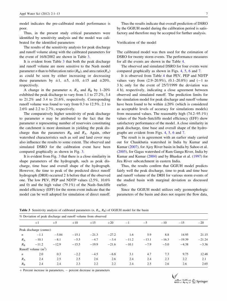
identified by sensitivity analysis for the event of 16/8/2002

and the model was calibrated for the identified parameters.

The criteria for model evaluation involve the following:

• Percentage error in simulated volume (PEV)

• Percentage error in simulated peak (PEP), and

• Net difference of observed and simulated time to peak

(NDTP), as given below:

PEV ¼ ðVolo � VolcÞVolo

� 100 ð9Þ

PEP ¼ ðQpo � QpcÞQpo

� 100 ð10Þ

NDTP ¼ ðTpo � TpcÞ ð11Þ

Volo is the observed runoff volume (m3); Volc is the

computed runoff volume (m3); Qpo is the observed peak

discharge (m3/s); Qpc is the computed peak discharge (m3/s);

Tpo is the time to peak of observed discharged (h); and Tpc is

the time to peak of computed discharge (h). The prediction

of overall performance of the model was assessed using

Nash–Sutcliffe model efficiency (EFF) criterion (Nash and

Sutcliffe 1970), recommended by ASCE Task Committee

(1993)

EFF ¼

Pno

i¼1

Qoi � Qo

� �2�Pno

i¼1

Qci � Qoið Þ2

Pno

i¼1

Qoi � Qo

� �2ð12Þ

where Qoi is ith ordinate of the observed discharge (m3/s);

Qo is the mean of the ordinates of observed discharge (m3/s);

Qci is ith ordinate of the computed discharge (m3/s).

After model prediction, the dataset was grouped into 10

classes. Each class represents the values that fall into the

incremental domains which are determined by dividing the

difference of highest and lowest data value with 10. The

probability of these periods are plotted and matched with

common distribution functions to identify the better mat-

ched one which was taken as the representative of the

dataset. Predictions from the two models and actual data

were used to identify the best fit density function.

Result and discussion

Morphometric analysis of the basin

The geomorphologic parameters were computed graphi-

cally by plotting number of streams, stream length and

stream area versus the order of the stream and finding the

slope of the best fit equation. The values of bifurcation

ratio (RB), length ratio (RL), area ratio (RA) and length of

highest order stream (LX) were estimated as RB = 3.5,

RL = 2.2 and RA = 4.5, LX= 22.6 km and RB = 3.4,

RL = 2.4, RA = 3.9 and LX = 22.1 for the two scales

(1:250,000) and (1:50,000), respectively (Table 2). It may

be noted that these ratios lie in the ranges of values

observed for natural basins wherein RB ranges between 3

and 5, RL ranges between 1.5 and 3.5 and RA ranges

between 3 and 6 (Smart 1972).

Velocity and effective rainfall intensity relationship

The following relationship was obtained between velocity

and effective rainfall intensity

V ¼ 1:097i0:416r R2 ¼ 0:9

� �for 0:9\ir\7 ð13Þ

where V is the flow velocity in m/s and ir is the excess

rainfall intensity in mm/h. The above set of equations was

used for determining the flow velocity corresponding to the

average excess rainfall intensity of a particular storm event.

Calibration and sensitivity analysis of the model

The moderately high value of PEV (4.7%), high value of

PEP (21.2%) and low value of Nash–Sutcliffe model effi-

ciency (58.2%) for simulation of runoff with pre-calibrated

Table 2 Geomorphological

characteristics of the

Dulung-Nala River basin

Scale Stream

order (u)

total number

of streams (Nu)

mean stream

length (Lu) (km)

Mean stream area

of order u (Au) (km2)

Geomorphologic

parameters

(dimensionless)

1:250,000 1 32 3.4 8.74 RB = 3.5

2 14 2.9 39.9 RL = 2.2

3 3 7.9 213.5 RA = 4.5

4 1 22.6 802

1:50,000 1 201 0.6 2.2 RB = 3.4

2 58 1.1 11.9 RL = 2.4

3 18 2.8 35.8 RA = 3.9

4 2 13.3 380.3

5 1 22.1 802.2


123

model indicates the pre-calibrated model performance is

poor.

Thus, in the present study critical parameters were

identified by sensitivity analysis and the model was cali-

brated for the identified parameters

The results of the sensitivity analysis for peak discharge

and runoff volume along with the calibrated parameters for

the event of 16/8/2002 are shown in Table 3.

It is evident from Table 3 that both the peak discharge

and runoff volume are more sensitive to the Nash model

parameter n than to bifurcation ratio (RB), and area ratio(RA)

as could be seen by either increasing or decreasing

these parameters by ±1, ±5, ±10, ±15 and ±20%,

respectively.

A change in the parameter n, RA and RB by 1–20%

exhibited the peak discharge to vary from 1.1 to 27.2%, 3.4

to 21.2% and 3.4 to 21.6%, respectively. Corresponding

runoff volume was found to vary from 0.3 to 12.5%, 2.1 to

2.6% and 2.2 to 2.7%, respectively.

The comparatively higher sensitivity of peak discharge

to parameter n may be attributed to the fact that the

parameter n representing number of reservoirs constituting

the catchment is more dominant in yielding the peak dis-

charge than the parameters RB and RA. Again, other

watershed characteristics such as soil and land cover may

also influence the results to some extent. The observed and

simulated DSRO for the calibration event have been

compared graphically as shown in Fig. 3.

It is evident from Fig. 3 that there is a close similarity in

shape parameters of the hydrograph, such as peak dis-

charge, time base and overall shape of the hydrograph.

However, the time to peak of the predicted direct runoff

hydrograph (DRH) occurred 2 h before that of the observed

one. The low PEV, PEP and NDTP values (2.5%, 10.6%

and 0) and the high value (79.1%) of the Nash–Sutcliffe

model efficiency (EFF) for the storm event indicate that the

model can be well adopted for simulation of direct runoff.

Thus the results indicate that overall prediction of DSRO

by the GGIUH model during the calibration period is satis-

factory and therefore may be accepted for further analysis.

Verification of the model

The calibrated model was then used for the estimation of

DSRO for twenty storm events. The performance measures

for all the events are shown in the Table 4.

The observed and simulated DSRO for four events were

compared graphically as shown in Figs. 4, 5, 6 and 7.

It is observed from Table 4 that PEV, PEP and NDTP

values vary from (2.9–20.9%), (0.1–20.8%) and (-1 to

3 h; only for the event of 25/7/1999 the deviation was

4 h), respectively, indicating a close agreement between

observed and simulated runoff. The prediction limits for

the simulation model for peak discharge and runoff volume

have been found to be within ±20% (which is considered

as acceptable levels of accuracy for simulations models)

from measured values. The reasonably high (74.2–95.1%)

values of the Nash–Sutcliffe model efficiency (EFF) show

satisfactory performance of the model. A close similarity in

peak discharge, time base and overall shape of the hydro-

graphs are evident from Figs. 4, 5, 6 and 7.

The result is in agreement with an earlier study carried

out for Chaukhutia watershed in India by Kumar and

Kumar (2007), for Ajoy River basin in India by Sahoo et al.

(2005), for Gagas watershed of Ram Ganga River, India by

Kumar and Kumar (2004) and by Bhaskar et al. (1997) for

Jira River subcatchment in eastern India.

Thus, the results confirm that GGIUH model predicts

fairly well the peak discharge, time to peak and time base

and runoff volume of the DRH for various storm events of

the studied basin with marginal deviation as discussed

earlier.

Since the GGIUH model utilizes only geomorphologic

parameters of the basin and does not require the flow data,

Table 3 Sensitivity analysis of calibrated parameters (n, RA, RB) of GGIUH model for the basin

% Deviation of peak discharge and runoff volume from observed

?1 ?5 ?10 ?15 ?20 -1 -5 -10 -15 -20

Peak discharge (cumec)

n -1.1 -5.84 -15.1 -21.3 -27.2 1.6 5.9 8.8 14.95 21.15

RA -10.1 -8.1 -5.5 -4.7 -3.4 -11.2 -13.1 -16.3 -19.39 -21.24

RB -11.2 -12.9 -15.5 -19.9 -21.6 -10.1 -7.9 -5.0 -4.38 -3.36

Runoff volume (m3)

n 2.0 0.3 -2.2 -4.5 -6.8 3.1 4.7 7.3 9.75 12.48

RA 2.4 2.5 2.5 2.6 2.6 2.4 2.4 2.3 2.2 2.1

RB 2.4 2.4 2.3 2.2 2.2 2.4 2.5 2.6 2.6 2.65

? Percent increase in parameters, - percent decrease in parameters


123

this model can be applied for predicting DRH for ungauged

basins.

Comparative performance analysis of GGIUH model

for two topographic map scales of 1:50,000

and 1:250,000

The DSRO hydrographs were computed using the GGIUH

model at two map scales (viz. 1:50,000 and 1:250,000) in

order to study the effect of the basin map scale on the per-

formance of the GGIUH based model. The peak (QP) and

time to peak (TP) of the direct surface runoff hydrographs of

observed and as derived by the GGIUH model for the map

scales 1:250,000 and 1:50,000 are shown in Table 5.

It is observed that the peak flow (qp) as estimated by the

model is higher (ranges between 7.1 and 20.3%) at map

scale 1:50,000 than that at map scale 1:250,000. While

Time to peak (tp) as estimated by the model is lower

(ranges between 0 and 16.7%) at map scale 1:50,000 than

that at map scale 1:250,000.

It is revealed from Tables 4 and 6 that the EFF, NDTP

and PEP are almost same for both the map scales. How-

ever, PEV is slightly lower for basin map scale 1:50,000

than that of 1:250,000. These results indicate that the

GGIUH model yields comparable performance for the two

map scales. Hence, a lower map scale of 1:250,000 can

also be used to estimate the DSRO hydrographs for un-

gauged basin with reasonable accuracy.

It may be noted that Sahoo et al. (2005) in course of their

study in Ajoy River basin in India concluded that smaller

basin map scales can be used to estimate geomorphological

parameters and correspondingly DSRO hydrographs.

Comparative performance analysis of GGIUH model

and ANN

The neural network model trained with CGD algorithm has

been used to predict DSRO hydrographs for various storm

Fig. 3 Observed and calibrated

DSRO hydrographs by GGIUH

model for the event 16/8/2002

Table 4 Performance measures of GGIUH model for storm events

(basin map scale 1:50,000)

Events PEP PEV NDTP EFF

14/9/1994 10.5 20.6 2 84.5

6/9/1995 20.7 20.9 3 77.7

11/10/1995 -0.1 17.1 3 83.2

21/7/1999 -4.4 10.5 2 85.2

28/8/1997 -3.5 12.8 3 74.6

16/8/1999 5.3 9.1 3 79.4

6/9/2002 -6.2 7.7 2 84.6

24/8/2002 -9.6 5.4 3 74.2

8/6/1997 -16.2 15.0 3 82.1

20/9/2000 -3.2 19.6 3 90.6

25/7/1999 -7.2 15.5 4 87.3

7/8/1999 -7.1 18.3 3 88.5

23/6/1996 1.7 20.1 3 80.6

19/7/1998 6.8 20.7 1 84.1

23/6/1999 -3.3 -10.9 1 95.2

25/6/2004 -14.9 2.9 -1 80.9

Fig. 4 Observed and simulated DSRO hydrographs by GGIUH

model for two basin map scales for the event 6/9/2002


123







Table 5 Peak discharge and time to peak of the observed and the

GGIUH model DSRO hydrographs at two basin map scales 1:250,000

and 1:50,000

Event date Observed GGUIH model

Scale 1:50,000 Scale 1:250,000

QP

(cumec)

TP

(h)

QP

(cumec)

TP

(h)

QP

(cumec)

TP

(h)

14/9/1994 220.9 8 197.7 6 179.9 7

6/9/1995 175.8 8 139.1 5 126.8 6

11/10/1995 160.9 8 161.1 5 145.8 6

21/7/1999 154.8 9 161.6 7 146.7 8

28/8/1997 288.9 8 298.9 5 277.6 6

16/8/1999 146.9 10 139.1 7 126.6 7

6/9/2002 156.8 9 166.6 7 151.2 8

24/8/2002 139.3 8 152.7 5 138.5 6

6/8/1997 549.5 10 638.5 7 602.5 8

20/9/2000 165.0 9 170.4 6 153.8 6

25/7/1999 133.8 9 143.5 5 130.5 6

7/8/1999 703.6 10 753.7 7 690.6 7

23/6/1996 59 8 57.9 5 52.9 5

19/7/1998 30 7 27.9 6 23.6 6

23/6/1999 60.9 7 62.9 6 57.5 6

25/6/2004 20.2 8 23.2 9 18.5 9

Table 6 Performance measures of GGIUH model for storm events

(basin map scale 1:250,000)

Events PEP PEV NDTP EFF

14/9/1994 18.6 29.4 1 86.8

6/9/1995 27.9 23.4 2 69.7

11/10/1995 9.4 15.8 2 83.6

21/7/1999 5.3 9.1 1 95.9

28/8/1997 3.9 11.3 2 77.3

16/8/1999 13.8 7.3 3 92.1

6/9/2002 3.6 6.4 1 96.3

24/8/2002 0.6 3.7 2 73.4

6/8/1997 -9.7 14.4 2 84.8

20/9/2000 6.8 18.1 3 87.5

25/7/1999 2.5 13.9 3 86.2

7/8/1999 1.9 17.2 3 85.8

23/6/1996 10.2 19.2 3 82.3

19/7/1998 21.4 18.2 1 87.5

23/6/1999 5.6 -12.3 1 92.2

25/6/2004 8.4 8.3 -1 79.3


123

Fig. 8 DSRO hydrographs

simulated by GGIUH model

and ANN model for the event

6/9/2002




21/7/1999




11/10/1995

10 Appl Water Sci (2012) 2:1–13

123

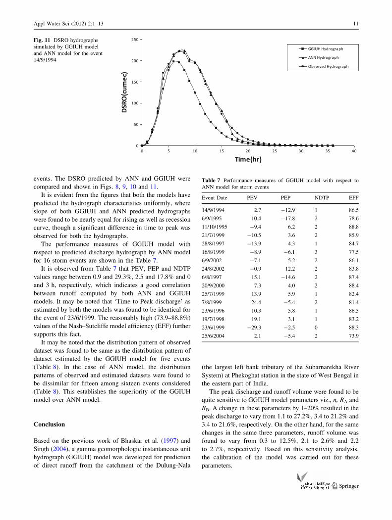
events. The DSRO predicted by ANN and GGIUH were

compared and shown in Figs. 8, 9, 10 and 11.

It is evident from the figures that both the models have

predicted the hydrograph characteristics uniformly, where

slope of both GGIUH and ANN predicted hydrographs

were found to be nearly equal for rising as well as recession

curve, though a significant difference in time to peak was

observed for both the hydrographs.

The performance measures of GGIUH model with

respect to predicted discharge hydrograph by ANN model

for 16 storm events are shown in the Table 7.

It is observed from Table 7 that PEV, PEP and NDTP

values range between 0.9 and 29.3%, 2.5 and 17.8% and 0

and 3 h, respectively, which indicates a good correlation

between runoff computed by both ANN and GGIUH

models. It may be noted that ‘Time to Peak discharge’ as

estimated by both the models was found to be identical for

the event of 23/6/1999. The reasonably high (73.9–88.8%)

values of the Nash–Sutcliffe model efficiency (EFF) further

supports this fact.

It may be noted that the distribution pattern of observed

dataset was found to be same as the distribution pattern of

dataset estimated by the GGIUH model for five events

(Table 8). In the case of ANN model, the distribution

patterns of observed and estimated datasets were found to

be dissimilar for fifteen among sixteen events considered

(Table 8). This establishes the superiority of the GGIUH

model over ANN model.

Conclusion

Based on the previous work of Bhaskar et al. (1997) and

Singh (2004), a gamma geomorphologic instantaneous unit

hydrograph (GGIUH) model was developed for prediction

of direct runoff from the catchment of the Dulung-Nala

(the largest left bank tributary of the Subarnarekha River

System) at Phekoghat station in the state of West Bengal in

the eastern part of India.

The peak discharge and runoff volume were found to be

quite sensitive to GGIUH model parameters viz., n, RA and

RB. A change in these parameters by 1–20% resulted in the

peak discharge to vary from 1.1 to 27.2%, 3.4 to 21.2% and

3.4 to 21.6%, respectively. On the other hand, for the same

changes in the same three parameters, runoff volume was

found to vary from 0.3 to 12.5%, 2.1 to 2.6% and 2.2

to 2.7%, respectively. Based on this sensitivity analysis,

the calibration of the model was carried out for these

parameters.




14/9/1994

Table 7 Performance measures of GGIUH model with respect to

ANN model for storm events

Event Date PEV PEP NDTP EFF

14/9/1994 2.7 -12.9 1 86.5

6/9/1995 10.4 -17.8 2 78.6

11/10/1995 -9.4 6.2 2 88.8

21/7/1999 -10.5 3.6 2 85.9

28/8/1997 -13.9 4.3 1 84.7

16/8/1999 -8.9 -6.1 3 77.5

6/9/2002 -7.1 5.2 2 86.1

24/8/2002 -0.9 12.2 2 83.8

6/8/1997 15.1 -14.6 2 87.4

20/9/2000 7.3 4.0 2 88.4

25/7/1999 13.9 5.9 1 82.4

7/8/1999 24.4 -5.4 2 81.4

23/6/1996 10.3 5.8 1 86.5

19/7/1998 19.1 3.1 1 83.2

23/6/1999 -29.3 -2.5 0 88.3

25/6/2004 2.1 -5.4 2 73.9

Appl Water Sci (2012) 2:1–13 11

123

The Nash–Sutcliffe model efficiency (EFF) criterion,

percentage error in volume (PEV), the percentage error in

peak (PEP), and net difference of observed and simulated

time to peak (NDTP) which were used for performance

evaluation of the model for 16 storm events, have been

Table 8 Probability distribution function (PDF) for observed data,

GGIUH and ANN model

Events Distribution Parameters

24/8/2002

ANN Fatigue Life a = 3.2654, b = 28.749

GGIUH Weibull a = 0.22344, b = 15.016

Observed Beta a1 = 0.16874, a2 = 0.47736

a = -6.6232E-15, b = 588.4

6/9/2002


GGIUH Weibull a = 0.30488, b = 13.028

Observed Johnson SB c = 0.59908, d = 0.21162

k = 217.9, n = 0.93392

16/8/1999


GGIUH Power

Function

a = 0.17764, a = 4.5807E-15,

b = 142.73

Observed Power

Function

a = 0.21961, a = 4.1899E-16,

b = 182.6

28/8/1997

ANN Log-Logistic a = 0.57772, b = 3.7588

GGIUH Fatigue Life a = 4.2451, b = 3.5755

Observed Fatigue Life a = 3.4199, b = 6.4133

21/7/1999

ANN Power

Function

a = 0.32396, a = -0.64668,

b = 163.93

GGIUH Kumaraswamy a1 = 0.23789, a2 = 1.1198

a = -2.0097E-15, b = 230.0

Observed Beta a1 = 0.21517, a2 = 0.47141

a = -1.0805E-14, b = 154.79

11/10/1995

ANN Fatigue Life

(3P)

a = 3.9516, b = 6.8613,

c = -0.73036

GGIUH Weibull a = 0.21076, b = 3.527


6/9/1995

ANN Gamma (3P) a = 0.36791, b = 129.07,

c = -0.64668


Observed Dagum k = 9.2903E-4, a = 415.48,

b = 173.02

14/9/1994




23/6/1996

ANN Fatigue Life

(3P)

a = 1.7423, b = 0.86005,

c = -0.23972



Table 8 continued

Events Distribution Parameters

23/6/1999

ANN Pearson 5 (3P) a = 0.86984, b = 0.48389,

c = -0.32166

GGIUH Dagum k = 0.00438, a = 84.816, b = 64.218

Observed Beta a1 = 0.26942, a2 = 0.82488

a = -1.0362E-14, b = 60.935

25/6/2004

ANN Burr (4P) k = 1.5494, a = 0.78285

b = 0.65279, c = -0.1497



19/7/1998

ANN Beta a1 = 0.16686, a2 = 0.36355

a = -0.00203, b = 4.1239


Observed Kumaraswamy a1 = 0.21312, a2 = 0.8398

a = -1.9339E-14, b = 30.0

25/7/1999

ANN Beta a1 = 0.22439, a2 = 0.58132

a = -1.6000E-4, b = 6.5758


Observed Weibull a = 0.30715, b = 10.867

6/8/1997

ANN Fatigue Life

(3P)

a = 3.936, b = 1.8459, c = -0.16067

GGIUH Beta a1 = 0.15201, a2 = 0.46625

a = -6.6606E-15, b = 638.52

Observed Pearson 6 a1 = 0.27404, a2 = 1167.2,

b = 6.3967E?5

7/8/1999

ANN Beta a1 = 0.1366, a2 = 0.36814

a = 0.12512, b = 73.993


Observed Power

Function

a = 0.16874, a = 4.9068E-15,

b = 705.33

20/9/2000

ANN Johnson SB c = 0.83812, d = 0.23763

k = 20.959, n = -0.17622


Observed Kumaraswamy a1 = 0.19957, a2 = 1.0925

a = 1.9191E-15, b = 253.34

12 Appl Water Sci (2012) 2:1–13

123

found to range from 74.1 to 95.1%, 2.9 to 20.9%, 0.1 to

20.8% and -1 to 3 h (only for the event of 25/7/1999 the

deviation was 4 h) respectively, indicating a good perfor-

mance of the calibrated GGIUH model for prediction of

runoff hydrograph.

Again, ANN models were prepared and trained with three

different training algorithms to predict discharge hydrograph

using observed rainfall and discharge hydrograph.

Analysis of performance measures of GGIUH model,

with respect to predicted discharge hydrograph by ANN

model, reveals that the PEV, PEP, NDTP and EFF values

range between 0.9 and 29.3%, 2.5 and 17.8%, 0 and 3 h

and 73.9 to 88.8%, respectively, indicating comparable

performance of both ANN and GGIUH models.

Further, DSRO hydrographs computed using the

GGIUH model at two map scales (viz. 1:50,000 and

1:250,000) were found to yield comparable performance

indicating suitability of using lower map scale to estimate

the DSRO hydrographs. Thus, lower map scales may also

be employed for extraction of geomorphological para-

meters in case of non-availability of larger map scales

(1: 50,000). This would further minimize the extent of

labor and time involvement in estimating parameters and

this has a practical relevance to field engineers. In a study

in the Ajoy River basin in India, Sahoo et al. (2005)

reported that smaller basin map scales may be used to

estimate DSRO with reasonable accuracy. As GGIUH

model was found to predict the event distribution pattern

more efficiently than the ANN model, the supremacy of the

former over latter is evident. Thus, the GGIUH model

which does not use historical runoff data can be used for

the prediction of design floods from ungauged basins.

Open Access This article is distributed under the terms of the

Creative Commons Attribution License which permits any use, dis-

tribution and reproduction in any medium, provided the original

author(s) and source are credited.

References

Ahmad S, Simonovic SP (2005) An artificial neural network model

for generating hydrograph from hydro-meteorological parame-

ters. J Hydrol 315:236–251

ASCE Task Committee (2000) Application of artificial neural

networks in hydrology. J. Hydrol Eng 5:115–123

Bhaskar NR, Parida BP, Nayak AK (1997) Flood estimation for

ungauged catchment using the GIUH. J Water Resour Plan

Manag ASCE 123:228–238

Chutha P, Dooge JCI (1990) The shape of parameters of the

Geomorphologic Unit hydrograph. J Hydrol 117:81–97

Hong W, Feng L (2008) On hydrologic calculation using artificial

neural networks. Appl Math Lett 21:453–458

Jain SK, Singh RD, Seth SM (2000) Design flood estimation using GIS

supported GIUH approach. Water Resour Manag 14:369–376

Kumar A, Kumar D (2004) Derivation of a kinematic-wave and

topographically based instantaneous unit hydrograph for a hilly

catchment. Hydrology J IAH 27:15–27

Kumar A, Kumar D (2007) A geomorphologic instantaneous unit

hydrograph model applied to the Chaukhutia watershed, India.

Hydrol J 30:65–76

Majumdar M, Barman RN, Jana BK, Roy PK, Mazumdar A (2009)

Application of neuro-genetic algorithm to determine reservoir

response in different hydrologic adversaries. J Soil Water Res

Inst Agric Econ Inf 4:17–27

Nash JE, Sutcliffe JV (1970) River flow forecasting through

conceptual models Part 1-A discussion of principals. J Hydrol

10:282–290

Neelakantan TR, Pundarikanthan NV (2000) Neural network based

simulation-optimization model for reservoir operation. J Water

Resour Plan Manag 126:57–64

Ray C, Klindworth KK (2000) Neural networks for agrichemical

vulnerability assessment of rural private wells. J. Hydrol Eng

5:162–171

Rodriguez-Iturbe I, Valdes JB (1979) The geomorphologic structure

of hydrologic response. Water Resour Res 15:1409–1420

Rodriguez-Iturbe I, Deroto G, Valdes JB (1979) Discharge response

analysis and hydrologic similarity: the interrelation between the

geomorphologic IUH and the storm characteristics. Water

Resour Res 15:1435–1444

Rodriguez-Iturbe I, Gonzalez-Sanabria M, Caamano G (1982) On the

climatic dependence of the IUH: a rainfall-runoff analysis of the

Nash model and the geomorphoclimatic theory. Water Resour

Res 4:887–903

Sahoo B, Chatterjee C, Raghuwanshi NS (2005) Runoff prediction in

ungauged basins at different basin map scales. Hydrol J

28:45–58

Sahoo B, Chatterjee C, Narendra S, Singh RR, Kumar R (2006) Flood

Estimation by GIUH-based Clark and Nash models. J Hydrol

Eng 11:515–525

Sherman LK (1932) Stream flow from rainfall by the unit-graph

method. Eng News Record 108:501–505

Singh SK (2004) Simplified use of gamma distribution/Nash model

for runoff modelling. J Hydrol Eng 9:240–243

Smart JS (1972) Channel networks, advances in hydrosciences. In:

Chow (ed), vol 8, Academic Press, New York, pp 305–346

Sorman AU (1995) Estimation of peak discharge using GIUH model

in Saudi Arabia. J Water Resour Plan Manag ASCE

121:287–293

Task Committee ASCE (1993) Criteria for evaluation of watershed

models. J Irrig Drain Eng 119:429–442

Troutman BM, Karlinger MR (1985) Unit hydrograph approximations

assuming linear How through topologically random channel

networks. Water Resour Res 21:743–754

Valdes JB, Fiallo Y, Rodriguez-Iturbo I (1979) A rainfall runoff

analysis of the geomorphologic IUH. Water Resour Res

15:1421–1434

Wooding RA (1965) A hydraulic model for the catchment-stream

problem: II. numerical solution. J Hydrol 3:268–282

Yen BC, Lee KT (1997) Unit hydrograph derivation for ungauged

watersheds by stream-order laws’. J Hydrol Eng ASCE 2:1–9

Zhang B, Govindaraju RS (2003) Geomorphology-based artificial

neural networks (GANNs) for estimation of direct runoff over

watersheds. J Hydrol 273:18–34

Zhang X, Srinivasan R, Van Liew M (2008) Multi-site calibration of

the SWAT model for hydrologic modeling. Trans ASABE

51:2039–2049

Appl Water Sci (2012) 2:1–13 13

123

A comparative study for prediction of direct runoff for a ...

Documents

Transcript of A comparative study for prediction of direct runoff for a ...