Research ArticleVolume 12 Issue 4 - October 2020DOI: 10.19080/OFOAJ.2020.12.555842

Oceanogr Fish Open Access JCopyright © All rights are reserved by Thanh Nguyen Trung

Thanh Nguyen Trung1*, Lars Robert Hole2, Tien Du Duc3 and Huan Nguyen Minh1

1VNU University of Science, Vietnam2Norwegian Meteorological Institute, Norway3Viet Nam National Center for Hydro-Meteorological Forecasting, Vietnam

Submission: September 01, 2020; Published: October 07, 2020

Corresponding author: Thanh Nguyen Trung, VNU University of Science, 334 Nguyen Trai Str, Thanh Xuan, 100000 Hanoi, Vietnam

Oceanogr Fish Open Access J 12(4): OFOAJ.MS.ID.5557842 (2020) 001

Introduction

The marine and atmospheric model’s accuracy mainly depends on the quality of the initial and boundary conditions, numeric, and physics of the model, and on the variation of the phenomena (e.g., chaos of atmosphere) [1-3]. In the wave prediction problem, the wave field is mainly calculated based on the wave–action balance equations (e.g., the WAVEWATCH III, simulating waves nearshore - SWAN, wave model - WAM) with the given initial and boundary conditions. There are two types of boundary conditions, including surface and open boundaries. The surface boundary is a field of meteorological factors (wind and pressure fields) extracted from meteorological forecasting models. For the open boundaries, the wave direction, period, wave height or wave spectrum from models or observations can be used at a limited area, such as the South China Sea - East Sea of Vietnam (SCS). There are two ways to determine the initial condition for the wave model: (i) The initial condition is the

state of the calm sea surface until the actual state of the sea surface is reached to continue calculating the forecast (for example, in the SCS, this process usually takes 48 to 72 h); and (ii) using the analysis wave field as the initial condition. This initial field can be either the observational data or the wave field from the previous forecast (the hot start running).

It is found that the errors of the initial conditions of models can be alleviated using data assimilation (DA) methods, from empirical methods (successive correction method, nudging) to statistical methods (optimal interpolation and variational (VAR) methods) and advanced methods (Kalman Filter—KF, Ensemble Kalman Filter—EnKF or Hybrid VAR/EnKF) [4-11]. The variational method uses Bayesian theory to find the optimal analysis state for a given/priori state (or the background or short-range forecast), deviation/innovation of the model, and limited-number-observations and the prior/predefined information

Abstract

The study uses the simulating waves nearshore (SWAN) model and ensemble Kalman filter (EnKF) method, which has been integrated in the Open Data Assimilation system, to assimilate wave observation data from the oil platform over the South China Sea - East Sea of Vietnam. A set of experiments with and without EnKF was established based on the different parameters, including ensemble size, standard deviation for the wind noise field, time correlation scale for boundaries updating processes, and the horizontal correlation scale in covariance derivation. Compared to observation and re-analysis European Centre for Medium-Range Weather Forecasts (ECMWF) data, results showed improved forecasts on the significant wave height and other SWAN model variables with data assimilation. The experiments have clearly updated error forecast informa-tion of the model (positive bias) to the 24 hour forecast results. The significant sensitivities to both magnitude and distribution for increments of model analysis fields and for forecast results on spatial and time correlation scales show the importance of investigating more suitable EnKF parameters for specific area and observation applications.

Keywords: Ensemble Kalman Filter; South China Sea; SWAN; Open DA

A Case Study of Wave Forecast Over South China Sea Using SWAN Model and

Ensemble Kalman Filter Method

How to cite this article: Thanh N T, Lars R H, Tien D D, Huan N M. A Case Study of Wave Forecast Over South China Sea Using SWAN Model and Ensemble Kalman Filter Method. Oceanogr Fish Open Access J. 2020; 12(4): 555842. DOI: 10.19080/OFOAJ.2020.12.555842002

Oceanography & Fisheries Open access Journal

of the background and observations (Gaussian distribution of background and observation covariance errors). Due to the limit of the priori error statistics from a prescribed source, as it relies heavily on the system, the ensemble-based DA methods (e.g., EnKF) retrieve it from an ensemble so that the use of linearized models becomes unnecessary [12].

Several DA applications for oceanographical problems can be listed here. While a successive correction method or statistical interpolation (SI) has been widely used in atmospheric and wave models by various meteorological centers worldwide, Emmanoui examined ways to improve this method to assimilate altimeter satellite data (from the European Space Agency ESA-ENVISAT) in the WAM model, and the result for the impact on wave forecasting in the Indian Ocean is much more considerable than in isolated areas [13]. More advances in using variational methods have been applied in Hasselmann [8] to the inversion problem with synthetic aperture radar (SAR) data by extending the cost function with a cutoff error term.

During wave forecast (large-scale wave model), the assimilation procedure was applied every time new observational data were available. This method was also revised in Yang-Ming [6] and has been extended more for the wave spectra from pitch-and-roll buoy data (a one-dimensional wave spectrum compared to a full two-dimensional wave spectrum of inverted SAR spectrum in the original Hasselmann work). More variational-based DA applications can be found with the validations of individual numerical adjoint procedures in Orzech [10] for a nearshore wave model and can be applied for the public domain of the SWAN model.

The main issue in forcing problems is that the wind sea/wave quickly loses memory of its initial state and therefore needs forecast range assimilation types along, such as the KF approach [14]. Yoon [11] developed a wave DA scheme based on KF combined with a nonlinear wave model. A number of experiments had been carried out using the synthetic data with noise for one-dimensionally propagating irregular waves, and the results showed that the estimated free surface elevation using the present DA scheme matched well the numerical solution of the nonlinear wave model in the absence of noise. The developed DA scheme can clearly improve the stability of the wave prediction system in comparison with that based on a purely numerical DA scheme. Evensen [15] proposed EnKF in which the background covariance error matrix can be estimated by the spread information of ensemble forecasting systems, for example, Serpoushan [16] using the Open Data Assimilation (OpenDA) toolbox with an EnKF option to improve the wave simulation for the SWAN model with wave data (significant wave height—SWH and peak wave period) recorded at five stations in the Persian Gulf.

Further developing the EnKF method, Lei [9] used an ensemble-based approach (ensemble optimal interpolation or extension of ensemble Kalman smoother—EnKS, more detail

in Evensen [17]) to assimilate altimeter SWH with a number of different observations from satellites (Jason-1 and 2 and ENVISAT) and buoys in the Wave Watch III model for the SCS. Results showed that this ensemble-based assimilation scheme provided as many positive outcomes as those of other previous schemes; therefore, it helps to alleviate the computational costs in practice.

The SCS and the focus area of this study is located over the west of the Pacific Ocean and surrounded by the island of Taiwan and the Philippines islands in the east; the Indonesian islands (Borneo, Sumatra) and the Malaysian Peninsula in the south and southeast; and the Indochina peninsula in the west and Southern China mainland in the north. With an area of about 3,400,000 km2, the average depth is ~1 km, and the maximum depth is ~5 km [18]. Many studies have been carried out for wave simulations, forecasts and using the observation data from satellites to enhance the quality of initial conditions over the SCS [18-20]. The errors of the wave height forecast can be amplified, especially during a tropical cyclone or strong northern winds over the SCS [21].

By using the wave observation of an oil platform over the SCS, this study investigated the capabilities of DA for wave forecast. This research applied the EnKF method, which already integrated in the OpenDA toolbox for the SWAN model. The remainder of the paper is organized as follows. The next section describes an overview of EnKF, the OpenDA toolbox, the SWAN model, the data, and the experimental design. The main results are discussed in Section 3, and conclusions are given in the final section.

Methodology, Data, and Experiment Designs

EnKF Algorithm and the OpenDA Toolbox

Hong and Kalnay [22] summarized the DA process as the finding of the best combination of the model forecast fx (also called as background fields) and the observation 0y to generate the improved initial condition or analysis state ax as:

0( ( ))a f fx x K y H x= + − (1)

where H is the forward observation operator (converting/interpolating model variables to observation space) If we define that fP and are the error covariance matrices for the forecast and observation and H is the linear perturbation of H then the weighting matrix K is given by Kalman gain formula:

1( )f T f TK P H HP H R −= + (2)

According to Evensen [15], if we have forecasts or an ensemble forecast with size and denoted as ( )

fe Kx k=1,2,… and the ensemble

mean fex− then the forecast error matrix can be estimated by:

1 ( ) ( )

1( )( )

1f m f f f f T

k e K e e KP x x x xem− −

=∑ − −−

� (3)

In this study, we used the pre-build EnKF procedures of OpenDA package for a wave forecast mode (described in the next

How to cite this article: Thanh N T, Lars R H, Tien D D, Huan N M. A Case Study of Wave Forecast Over South China Sea Using SWAN Model and Ensemble Kalman Filter Method. Oceanogr Fish Open Access J. 2020; 12(4): 555842. DOI: 10.19080/OFOAJ.2020.12.555842003

Oceanography & Fisheries Open access Journal

section). Developed by Verlaan et al. [23] of the Delft University of Technology in the Netherlands, OpenDA is a generic toolbox to provide many typical efficient DA schemes (e.g., ensemble-or variational-based approaches) which is independently compatible with the models, including the SWAN model in this study. Following OpenDA’s document, certain interfaces are defined in OpenDA to communicate to outside models which need to go through assimilation procedures [23].

There are some typical ways to generate the ensemble forecast, including using different model parameters or different models with the same forcing or one model but with different forcing (by adding noise to a given forcing). In this study with the OpenDA toolbox, the wave forecast is mainly dependent on wind forcing, and the adding noise to the given wind fields will be used to generate different wind boundaries. The wind effect in source/sink parts in wave action equations (denoted as γ ) is updated to surface boundaries depending on the time correlation scale, which can be described as the following equation for time step ith:

1 1i i iγ αγ µ− −= + (4)

where t

e τα−

=� , t� is the time step, τ is the time correlation

scale, and 1iµ − is noise having a Gaussian standard deviation 21µσ σ α= − with a given standard deviation for wind fields. In

addition to the model error generated by the wind forcing noise, an observation error can also be generated the same way by adding a Gaussian noise to observation when it is updated. Another aspect of assimilation is the practical computations of the covariance matrix. OpenDA uses the horizontal correlation scale () in deriving the i row and j column (denote as ij) covariance element ( ,covi j )of the covariance matrix as in the following equation:

1 ( , )22

,covii jj

hscalei j e

δ

σ−

= × (5)

where ( , )ii jjδ is the distance between the ii and jj points (in spherical space). Based on the main parameters, including ensemble size, time correlation scale, horizontal correlation scale, and standard deviation of noise, a few EnFK experiments is setup and listed in Subsection 2.4 of this section.

SWAN Model Description

The study uses the SWAN model for wave forecasts version 41.10. This is a third-generation spectral wave model to simulate and forecast waves generated by surface gravity waves. SWAN integrates with both finite difference and finite element schemes in all dimensions (time, geographic space, and spectral space) for the action balance equation (Booij [24]). The model can be downloaded via the following link: https//www.swanmodel.sourceforge.net/.

Data

Bathymetry Data

Depth and shoreline data for SCS are Earth Topography—ETOPO1, which was collected from NOAA [25]. Illustrated in Figure 1, the study domain is the entire SCS stretching from 1.5° to 25° N (from 150,000 to 2,800,000 in UTM 48, projection zone 105th) and 99° to 121° E (−150,000 to 2,200,000 in UTM 48, projection zone 105th). The study domain used unstructured grids with 10km of gridline in the nearshore areas and 50km of gridline for the offshore areas. The total number of grid cells are 12,858, which were generated by ADCIRC software version 10.0 [26].

Figure 1: Depth and grid structure over the study area and position of MSP1 observation station (marked as red dot).

How to cite this article: Thanh N T, Lars R H, Tien D D, Huan N M. A Case Study of Wave Forecast Over South China Sea Using SWAN Model and Ensemble Kalman Filter Method. Oceanogr Fish Open Access J. 2020; 12(4): 555842. DOI: 10.19080/OFOAJ.2020.12.555842004

Oceanography & Fisheries Open access Journal

Initial Conditions, Boundary Conditions, and Driving Wind Data

For the wave boundary, this study used three open boundaries for waves, including:(i) the Taiwan Strait (marked as 1 in Figure 1) in the north, connected to the Pacific Ocean; (ii) the Bashi Strait (marked as 2 in Figure 1) in the east, connected to the Pacific Ocean; and (iii) the Strait of Malacca (marked as 3 in Figure 1) in the south, connected to the Indian Ocean. The initial conditions were used from previous running (the hot-start setup) and the wind data were taken from wind forecast fields of the global CFS model of the National Center for Environmental Forecasting (NCEP) [27,28], with a horizontal resolution of 0.2 × 0.2 degrees and updated every 1 h, and were converted into UTM 48 projections [29].

Case Study and Observational Data

The period from 16 September 2013 to 20 September 2013 was selected in this research to study the performances of EnKF with single point observation. There was a tropical depression (TD) over the study area for this period (18W TD according to Joint Typhoon Warning Center—JTWC [30]). Formed in SCS, this TD had moved to the west and landed to the middle coastal of Vietnam. Wave observational data for the assimilation experiments were collected from an oil platform named MSP1 of

VietSovPetro Company [31], with a temporal resolution of 1h. This station is located offshore of Vung Tau City, which is about 150km southeast of the coast and marked as the red point in Figure 1. In Table 1, the details of wave observation from MSP1 from 16 September 2013 to 20 September 2013 are shown. In Table 1, the re-analysis of the ECMWF data is also provided for reference but only available for every 6h.

Experimental Designs

As mentioned in Subsection 2.1 of this section, by use of the OpenDA toolbox, the experiments were easily designed based on the different selections of the main factors affecting the DA process, including: (i) the horizontal correlation scale (from Exp01 to Exp05; (ii) the time correlation scale (Exp03, Exp08, Exp09); (iii) the number of ensemble members (Exp03, Exp10); and the (iv) standard deviation of noise for the wind boundary updating processes (Exp03, Exp06, Exp07). Details of all ensemble experiments are presented in Table 2. For all EnKF experiments, the standard deviation of observational noise was set to 0.1m and updated every 1 h. In the EnKF experiment, the observation was updated from 00z 16 September 2013 to 23z 18 September 2013 and the forecast time is from 00z 19 September 2013 to 23z 20 September 2013.

Table 1: Wave height observation from MSP1 station and interpolated values from re-analysis data from ECMWF. The unit is m.

Time MSP1 ECMWF Time MSP1 ECMWF Time MSP1 ECMWF

20130916.00 1.26 1.26 20130918.00 1.62 1.97 20130920.00 1.11 1.38

20130916.01 1.26 20130918.01 1.68 20130920.01 1.04

20130916.02 1.26 20130918.02 1.77 20130920.02 0.99

20130916.03 1.26 20130918.03 1.80 20130920.03 1.00

20130916.04 1.28 20130918.04 1.81 20130920.04 1.12

20130916.05 1.28 20130918.05 1.79 20130920.05 1.29

20130916.06 1.28 1.25 20130918.06 1.74 1.97 20130920.06 1.41 1.39

20130916.07 1.28 20130918.07 1.72 20130920.07 1.45

20130916.08 1.28 20130918.08 1.67 20130920.08 1.39

20130916.09 1.28 20130918.09 1.62 20130920.09 1.38

20130916.10 1.29 20130918.10 1.62 20130920.10 1.35

20130916.11 1.28 20130918.11 1.64 20130920.11 1.31

20130916.12 1.21 1.4 20130918.12 1.63 1.91 20130920.12 1.27 1.42

20130916.13 1.14 20130918.13 1.55 20130920.13 1.27

20130916.14 1.08 20130918.14 1.49 20130920.14 1.31

20130916.15 1.07 20130918.15 1.51 20130920.15 1.33

20130916.16 1.05 20130918.16 1.59 20130920.16 1.38

20130916.17 1.04 20130918.17 1.66 20130920.17 1.4

20130916.18 1.02 1.21 20130918.18 1.69 1.75 20130920.18 1.39 1.39

20130916.19 1.02 20130918.19 1.69 20130920.19 1.32

20130916.2 1.03 20130918.20 1.73

20130916.21 1.09 20130918.21 1.76 20130920.21 1.17

How to cite this article: Thanh N T, Lars R H, Tien D D, Huan N M. A Case Study of Wave Forecast Over South China Sea Using SWAN Model and Ensemble Kalman Filter Method. Oceanogr Fish Open Access J. 2020; 12(4): 555842. DOI: 10.19080/OFOAJ.2020.12.555842005

Oceanography & Fisheries Open access Journal

20130916.22 1.13 20130918.22 1.75 20130920.22 1.06

20130916.23 1.18 20130918.23 1.71

20130917.00 1.21 1.31 20130919.00 1.72 1.71

20130917.01 1.24 20130919.01 1.75

20130917.02 1.28 20130919.02 1.78

20130917.03 1.29 20130919.03 1.77

20130917.04 1.29 20130919.04 1.83

20130917.05 1.29 20130919.05 1.86

20130917.06 1.29 1.39 20130919.06 1.86 1.58

20130917.07 1.34 20130919.07 1.83

20130917.08 1.38 20130919.08 1.85

20130917.09 1.38 20130919.09 1.85

20130917.10 1.29 20130919.10 1.84

20130917.11 1.2 20130919.11 1.84

20130917.12 1.12 1.5 20130919.12 1.89 1.84

20130917.13 1.09 20130919.13 1.92

20130917.14 1.15 20130919.14 1.91

20130917.15 1.29 20130919.15 1.84

20130917.16 1.51 20130919.16 1.76

20130917.17 1.69 20130919.17 1.68

20130917.18 1.83 1.71 20130919.18 1.60 1.57

20130917.19 1.85 20130919.19 1.52

20130917.20 1.84 20130919.20 1.40

20130917.21 1.77 20130919.21 1.36

20130917.22 1.69 20130919.22 1.27

20130917.23 1.61 20130919.23 1.22

Table 2: Ensemble settings in this research.

Convention Horizontal Correlation Scale (km)

Time Correlation Scale (hour) Size of Ensembles in EnKF Wind Noise (m/s)

Exp01 50 24 20 1.5

Exp02 100 24 20 1.5

Exp03 200 24 20 1.5

Exp04 500 24 20 1.5

Exp05 5000 24 20 1.5

Exp06 200 24 20 0.5

Exp07 200 24 20 2.5

Exp08 200 12 20 1.5

Exp09 200 36 20 1.5

Exp10 200 24 40 1.5

The non-using DA was denoted as the NoEnKF experiment. To reduce the uncertainties of wind driving data for SWAN in the NoEnKF experiment, the study still generated the ensemble forecast for this case, with 20 members and using a 1.5 m/s

standard deviation for wind noise. The time scale is 24h. Validation was carried out for the ensemble mean forecast of the EnKF experiment, including: (i) a comparison with the observation data from oil platform MSP1 hourly; and (ii) a comparison with

How to cite this article: Thanh N T, Lars R H, Tien D D, Huan N M. A Case Study of Wave Forecast Over South China Sea Using SWAN Model and Ensemble Kalman Filter Method. Oceanogr Fish Open Access J. 2020; 12(4): 555842. DOI: 10.19080/OFOAJ.2020.12.555842006

Oceanography & Fisheries Open access Journal

re-analysis ECMWF data every 6h at computing grid points. The validation of the experiments was based on common verification indexes, including BIAS and Root mean square error (RMSE). If we defined obs(i) as the observed value and fcst(i) as the forecast at time i, and N as the size of the sample:

BIAS is determined by the following formula:

1

1( ( ) ( ))N

iBIAS fcst i obs iN == −∑ (6)

RMSE is determined as:2

1

1( ( ) ( ))N

iRMSE fcst i obs iN == −∑ (7)

Results

General Performance

(a)

(b)

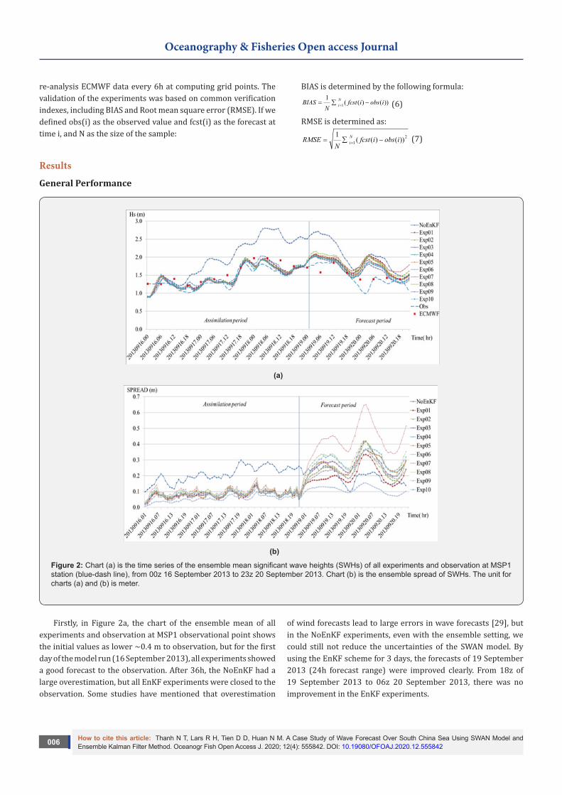
Figure 2: Chart (a) is the time series of the ensemble mean significant wave heights (SWHs) of all experiments and observation at MSP1 station (blue-dash line), from 00z 16 September 2013 to 23z 20 September 2013. Chart (b) is the ensemble spread of SWHs. The unit for charts (a) and (b) is meter.

Firstly, in Figure 2a, the chart of the ensemble mean of all experiments and observation at MSP1 observational point shows the initial values as lower ~0.4 m to observation, but for the first day of the model run (16 September 2013), all experiments showed a good forecast to the observation. After 36h, the NoEnKF had a large overestimation, but all EnKF experiments were closed to the observation. Some studies have mentioned that overestimation

of wind forecasts lead to large errors in wave forecasts [29], but in the NoEnKF experiments, even with the ensemble setting, we could still not reduce the uncertainties of the SWAN model. By using the EnKF scheme for 3 days, the forecasts of 19 September 2013 (24h forecast range) were improved clearly. From 18z of 19 September 2013 to 06z 20 September 2013, there was no improvement in the EnKF experiments.

How to cite this article: Thanh N T, Lars R H, Tien D D, Huan N M. A Case Study of Wave Forecast Over South China Sea Using SWAN Model and Ensemble Kalman Filter Method. Oceanogr Fish Open Access J. 2020; 12(4): 555842. DOI: 10.19080/OFOAJ.2020.12.555842007

Oceanography & Fisheries Open access Journal

The assimilation results and the forecast from the EnKF experiment show the large positive bias of the model for the period from 00z 17 September 2013 to 00z 19 September 2013 (assimilated period), and the EnKF updated these model error information (positive biases) to the initial fields, which can help to clearly reduce the model error for a 24h forecast range (00z 19 September 2013 to 00z 20 September 2013). For the period from 12z 19 September 2013 to 00z 20 September 2013, the model performed quite closely to the observation, but after this period, the sea state had changed by reducing the wave height, and all of the experiments could not catch this result. In fact, this is the typical result while applying the KF algorithm when the phenomena change quite suddenly, for example, when the air temperature changes by a cold surge or the onset of the rainy season [32, 33].

Even though there is no improvement for the forecast of the second day, Figure 2b shows the larger ensemble spread (estimated as the standard deviation of ensemble members to its ensemble mean) of most EnKF experiments (~0.2m to 0.4m), which can provide high proportions of ensemble members closer to observations than the NoEnKF forecast. Related to the ensemble spread, Figure 2b shows the stable spreads of NoEnKF around 0.2–0.3m and the lowest spreads in Exp06 relating small wind noise of 0.5m/s. The Exp10 with 40 members can provide the largest spreads, meaning the lowest errors of this experiment, compared to others.

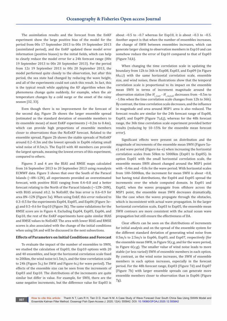
Figures 3 and 4 are the BIAS and RMSE maps calculated from 16 September 2013 to 20 September 2013 using reanalysis ECMWF data. Figure 3 shows that over the South of the Paracel Islands (~8N–12N), all experiments provided an overestimated forecast, with positive BIAS ranging from 0.4–0.8 and a better forecast relating to the North of the Paracel Islands (~12N–20N), with BIAS around ±0.2. In NoEnKF, the bias error is 0.6–0.9 for area 8N–12N (Figure 3a). When using EnkF, this error reduced to 0.3–0.5 for the experiments Exp04, Exp05, and Exp06 (Figure 3e–g) and 0.5–0.6 for Exp10 (Figure 3k). The same validations for the RMSE score are in Figure 4. Excluding Exp04, Exp05, Exp06, and Exp10, the rest of the EnKF experiments have quite similar BIAS and RMSE values to NoEnKF. The area with lower BIAS and RMSE scores is also associated with the change of the initial conditions when using DA and will be discussed in the next subsections.

Effects of Parameters on Initial Conditions and Forecast

To evaluate the impact of the number of ensembles to SWH, we studied the calculation of Exp03, the Exp10 options with 20 and 40 ensembles, and kept the horizontal correlation scale fixed to 200km, the wind noise to1.5m/s, and the time correlation scale to 24h (Figure 5c,j for SWH and Figure 6c,j for wave period). The effects of the ensemble size can be seen from the increments of Exp03 and Exp10. The distributions of the increments are quite similar but differ in value. For example, for SWH, there are the same negative increments, but the difference value for Exp03 is

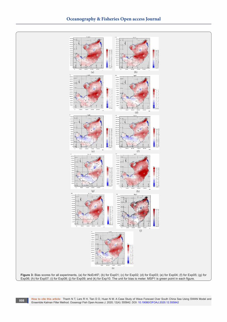
about −0.5 to −0.7 whereas for Exp10, it is about −0.3 to −0.5. Another aspect is that when the number of ensembles increases, the change of SWH between ensembles increases, which can generate larger closing to observation members in Exp10 and can somehow reduce the error of Exp10 compared to that of Exp03 (Figure 7d,k).

When changing the time correlation scale in updating the boundary from 12h to 36h in Exp08, Exp03, and Exp09 (in Figure 6h,c,i) with the same horizontal correlation scale, ensemble size, and wind noises, these illustrations show that the temporal correlation scale is proportional to its impact on the ensemble mean SWH in terms of increment magnitude around the observation station (the Hs_EnKF - Hs_NoEnKF decreases from −0.5m to −1.0m when the time correlation scale changes from 12h to 36h). By contrast, the time correlation scale decreases, and the influence in magnitude and area around MSP1 area is also reduced. The forecast results are similar for the 24h forecast range of Exp08, Exp03, and Exp09 (Figure 7i,d,j), whereas for the 48h forecast range, the 36h time correlation scale experiment provided better results (reducing by 10–15% for the ensemble mean forecast error).

Significant effects were present on distribution and the magnitude of increments of the ensemble mean SWH (Figure 5a–e) and wave period (Figure 6a–e) when increasing the horizontal correlation scales from 50km to 5000km (Exp01 to Exp05). In option Exp01 with the small horizontal correlation scale, the ensemble means SWH almost changed around the MSP1 point with −0.4m and −0.8s for the wave period. With horizontal scales from 100–5000km, the increment for mean SWH is about −0.8, but having total distributions, the Exp04 and Exp05 spread the increments over the whole computed domain. In Exp01 and Exp02, when the waves propagate from offshore across the MSP1 point, the ensemble mean SWH decreases dramatically, like the case when the waves propagate through the obstacles, which is inconsistent with actual wave propagation. In the larger horizontal correlation scale, Exp03 to Exp05, the ensemble mean SWH contours are more consistent with the actual ocean wave propagation but still ensure the effectiveness of DA.

Clear effects can be seen on the distributions of increments for initial analysis and on the spread of the ensemble system for the different standard deviation of generating wind noise from 0.5m/s to 2.5m/s in Exp06, Exp03, and Exp07, respectively (for the ensemble mean SWH, in Figure 5f,c,g, and for the wave period, in Figure 6f,c,g). The smaller value of wind noise leads to more stable (or less varied) SWH of ensemble members in each option. By contrast, as the wind noise increases, the SWH of ensemble members in each option increases, especially in the forecast period. For the 48h forecast range, Exp03 (Figure 7d) and Exp07 (Figure 7h) with larger ensemble spreads can generate more ensemble members closer to observation than in Exp06 (Figure 7g).

How to cite this article: Thanh N T, Lars R H, Tien D D, Huan N M. A Case Study of Wave Forecast Over South China Sea Using SWAN Model and Ensemble Kalman Filter Method. Oceanogr Fish Open Access J. 2020; 12(4): 555842. DOI: 10.19080/OFOAJ.2020.12.555842008

Oceanography & Fisheries Open access Journal

Figure 3: Bias scores for all experiments, (a) for NoEnKF; (b) for Exp01; (c) for Exp02; (d) for Exp03; (e) for Exp04; (f) for Exp05; (g) for Exp06; (h) for Exp07; (i) for Exp08; (j) for Exp09; and (k) for Exp10. The unit for bias is meter. MSP1 is green point in each figure.

(a) (b)

(d)

(e) (f)

(g) (h)

(j)

(k)

How to cite this article: Thanh N T, Lars R H, Tien D D, Huan N M. A Case Study of Wave Forecast Over South China Sea Using SWAN Model and Ensemble Kalman Filter Method. Oceanogr Fish Open Access J. 2020; 12(4): 555842. DOI: 10.19080/OFOAJ.2020.12.555842009

Oceanography & Fisheries Open access Journal

(c)

Figure 4: RMSE scores for all experiments, (a) for NoEnKF; (b) for Exp01; (c) for Exp02; (d) for Exp03; (e) for Exp04; (f) for Exp05; (g) for Exp06; (h) for Exp07; (i) for Exp08; (j) for Exp09; and (k) for Exp10. The unit for RMSE is meter. MSP1 is green point in each figure.

(a) (b)

(c) (d)

(e) (f)

(g) (h)

(i) (j)

How to cite this article: Thanh N T, Lars R H, Tien D D, Huan N M. A Case Study of Wave Forecast Over South China Sea Using SWAN Model and Ensemble Kalman Filter Method. Oceanogr Fish Open Access J. 2020; 12(4): 555842. DOI: 10.19080/OFOAJ.2020.12.5558420010

Oceanography & Fisheries Open access Journal

Figure 5: Increments of ensemble mean SWH (difference of assimilated fields and background) at 23z 18 September 2013: (a) for Exp01; (c) for Exp02; (b) for Exp03; (c) for Exp04; (d) for Exp05; (e) for Exp06; (f) for Exp07; (g) for Exp08; (h) for Exp09; and (i) for Exp10. The unit for Hs is meter. MSP1 is white point in each figure.

(b)(a)

(c) (d)

(e) (f)

(g) (h)

(i)(j)

How to cite this article: Thanh N T, Lars R H, Tien D D, Huan N M. A Case Study of Wave Forecast Over South China Sea Using SWAN Model and Ensemble Kalman Filter Method. Oceanogr Fish Open Access J. 2020; 12(4): 555842. DOI: 10.19080/OFOAJ.2020.12.5558420011

Oceanography & Fisheries Open access Journal

Figure 6: The same as Fig. 5 but for increments of ensemble mean wave period (T) at 23UTC 18 September 2013: (a) for Exp01; (b) for Exp02; (c) for Exp03; (d) for Exp04; (e) for Exp05; (f) for Exp06; (g) for Exp07; (h) for Exp08; (i) for Exp09; and (j) for Exp10. The unit for T is second. MSP1 is white point in each figure.

How to cite this article: Thanh N T, Lars R H, Tien D D, Huan N M. A Case Study of Wave Forecast Over South China Sea Using SWAN Model and Ensemble Kalman Filter Method. Oceanogr Fish Open Access J. 2020; 12(4): 555842. DOI: 10.19080/OFOAJ.2020.12.5558420012

Oceanography & Fisheries Open access Journal

Figure 7: Time series of ensemble—light grey lines for the all ensemble members, red lines for the ensemble mean SWHs, and blue-dash lines for observation at MSP1 station, from 00z 16 September 2013 to 23z 20 September 2013: (a) for NoEnKF; (b) for Exp01; (c) for Exp02; (d) for Exp03; (e) for Exp04; (f) for Exp05; (g) for Exp06; (h) for Exp07; (i) for Exp08; (j) for Exp09l and (k) for Exp10. The blue vertical line is for separating the assimilation period and forecast period. The unit is meter.

How to cite this article: Thanh N T, Lars R H, Tien D D, Huan N M. A Case Study of Wave Forecast Over South China Sea Using SWAN Model and Ensemble Kalman Filter Method. Oceanogr Fish Open Access J. 2020; 12(4): 555842. DOI: 10.19080/OFOAJ.2020.12.5558420013

Oceanography & Fisheries Open access Journal

Conclusion

This study used the EnKF assimilation method (integrated in the OpenDA system) to investigate the effects of observation (collected from an oil platform) on improving wave forecast with the SWAN model for the SCS for the period from 16 September 2013 to 20 September 2013. A set of numbers of assimilation experiments was established based on the changes of key parameters (ensemble size, standard deviation for wind noise fields, time correlation scales in boundaries updating processes, and horizontal correlation scale in covariance derivation) in EnKF of OpenDA. The wave height assimilation experiments showed the effects on the whole computing domain and for other model variables (e.g., the direction and period of wave).

The larger the horizontal correlation scale was, the more accurate SWH was in both the DA period and the forecasted period. However, the difference between the three options, whether the horizontal correlation scales are 200km, 500km, or 5000km, is insignificant. With a horizontal correlation scale of less than 200km, SWH distribution around the observation station fails to simulate the actual wave propagation. Thus, the horizontal correlation scale of 200km is enough to ensure the calculation results. During the DA period (00z 16 September 2013 to 23z 18 September 2013), the greater the wind noise, the more accurate the results, but the contrary is true in the forecasted period (00z 19 September 2013 to 23z 20 September 2013), meaning that the greater the wind noise, the more inaccurate the forecasted results. Thus, a wind noise of 1.5m/s is sufficient to ensure the results of DA and forecast.

During the DA period, the larger the time correlation scale was, the greater the error of SWH between simulation and observation; however, these errors do not differ significantly among options. By contrast, in the forecasted period, the larger the time correlation scales were, the more accurate the forecast. Thus, a time correlation scale of 36h ensures both the results of DA and forecast. It is noticeable in this study that the larger ensemble size is proportional with more accurate results during both the DA period and the forecasted period. However, a larger number of ensemble sizes require longer calculation time in practice.

Compared to both the observational station of the oil platform and the re-analysis of ECMWF data over the computing domain, the assimilation results and the forecasts from the EnKF experiments show the large positive bias of the model for the period from 00z 17 September 2013 to 00z 19 September 2013 (assimilated period), and the EnKF had updated these model errors (positive biases) to the initial fields, which can help to clearly reduce the model bias for the 24h forecast range (00z 19 September 2013 to 00z 20 September 2013).

For the period from 12z 19 September 2013 to 00z 20 September 2013, the simulations resembled quite closely the observations, but for the 48h forecast range, when the sea state

had changed quickly (reducing the wave height), it led to all of the assimilation experiments not being able to have a better adjustment compared to NoEnKF. The EnKF experiments showed a clear lower BIAS and RMSE score relating to the area around the assimilated observation position. Another aspect showing the non-linear behaviors in tuning parameters of EnKF is in Exp06. The Exp06 experiment had the smallest wind noise (leading small ensemble spreads) but can still reduce the BIAS and RMSE compared to other EnKF experiments and NoEnKF. More case studies and a combination of various observations in assimilation will be carried out to produce more comprehensive skill verifications in upcoming studies.

Acknowledgment

This research is supported by the Norwegian Agency for Development Cooperation through the contribution of L.R. Hole; and the research project of the Science and technology on integrated management of natural resources, protection of marine and island environments in the period of 2016-2020 under grant number TNMT.2018.06.03.

References1. Norton Lorenz Edward (1969) Atmospheric predictability as revealed

by naturally occurring analogues. Journal of Atmospheric Sciences 26: 636-646.

2. Norton Lorenz Edward (1969) Three approaches to atmospheric predictability. Bulletin of the American Meteorological Society 50(5): 345-349.

3. Inga Golbeck, Xin Li, Frank Janssen, Thorger Bruning, W Nielsen Jacob, et al. (2015) Uncertainty estimation for operational ocean forecast products a multi-model ensemble for the North Sea and the Baltic Sea. Ocean Dynamics 65: 1603-1631.

4. S Almeida, L Rusu, Soares C Guedes (2015) Application of the Ensemble Kalman Filter to a high-resolution wave forecasting model for wave height forecast in coastal areas. Maritime Technology and Engineering 1349-1354.

5. G Emmanouil, G Galanis, G Kallos, L A Breivik, H Heiberg, et al. (2007) Assimilation of radar altimeter data in numerical wave models: an impact study in two different wave climate regions. Annales Geophisicae 25(3): 581-595.

6. Yang-Ming Fan, Kuo-Ching Jao, Chia Chuen Kao, Dong-Jiing Doong, and Li-Chung Wu (2009) Numerical assimilation in nearshore spectral wave model, In Proceedings of the OCEANS 2009, MTS/IEEE Biloxi—Marine Technology for Our Future: Global and Local Challenges, Biloxi, MS, USA, 26-29.

7. George Galanis, George Emmanouil, C Chu Peter, and George Kallos (2009) A new methodology for the extension of the impact of data assimilation on ocean wave prediction. Ocean Dynamics 59: 523-535.

8. S Hasselmann, C Bruning, K Hasselmann, P Heimbach (1996) An improved algorithm for the retrieval of ocean wave spectra from synthetic aperture radar image spectra. Journal of Geophysical Research 101(C7): 615-629.

9. Cao Lei, Hou Yijun, Qi Peng (2015) Altimeter significant wave height data assimilation in the South China Sea using Ensemble Optimal Interpolation. Chinese Journal of Oceanology and Limnology 33(5): 1309-1319.

How to cite this article: Thanh N T, Lars R H, Tien D D, Huan N M. A Case Study of Wave Forecast Over South China Sea Using SWAN Model and Ensemble Kalman Filter Method. Oceanogr Fish Open Access J. 2020; 12(4): 555842. DOI: 10.19080/OFOAJ.2020.12.5558420014

Oceanography & Fisheries Open access Journal

10. D Orzech Mark, Jayaram Veeramony, Hans Ngodock (2012) A Variational Assimilation System for Nearshore Wave Modeling. Journal of Atmospheric and Oceanic Technology 30: 953-970.

11. Seongjin Yoon, Jinwhan Kim, Wooyoung Choi (2012) On data assimilation in a pseudo-spectral wave prediction model using a Kalman filter. In Proceedings of the Conference: 2012 Oceans - Yeosu, Yeosu, South Korea.

12. R N Bannister (2016) A review of operational methods of variational and ensemble-variational data assimilation. Royal Meteorological Society 143(703): 607-633.

13. Luigi Cavaleri and Paola Malanotte Rizzoli (1981) Wind wave prediction in shallow water: Theory and applications. Journal of Geophysical Research 86(C11): 10961-10973.

14. Paula Etala and Gerrit Burgers (1994) Real-Time Quality Control of Wave Observations in the North Sea. Journal of Atmospheric and Oceanic Technology 11: 1611-1624.

15. Geir Evensen (1994) Sequential data assimilation with a nonlinear quasi-geostrophic model using Monte Carlo methods to ear quasi-geostrophic model using Monte Carlo methods. Journal of Geophysical Research 99: 143-162.

16. Nima Serpoushan, Mostafa Zeinoddini, Maziar Golestani (2013) An Ensemble Kalman Filter Data Assimilation Scheme for Modeling the Wave Climate in Persian Gulf. In Proceedings of the ASME 2013 32nd International Conference on Ocean, Offshore and Arctic Engineering, Nantes, France.

17. Geir Evensen (1999) An Ensemble Kalman Smoother for Nonlinear Dynamics. American Meteorological Society 128: 1852-1867.

18. C Chu Peter, Yiquan Qi, Yuchun Chen, Ping Shi, and Qingwen Mao (2004) South China Sea Wind-Wave Characteristics. Part I: Validation of Wavewatch-III Using TOPEX/Poseidon Data. Journal of Atmospheric and Oceanic Technology 21: 1718-1833.

19. Zheng ChongWei, Zhuang Hui, Li Xin and Li XunQiang (2012) Wind energy and wave energy resources assessment in the East China Sea and South China Sea. Science China Press 55: 163-173.

20. Kohei Nagai, Shinji Kono, Dao Xuan Quang (1998) Wave Characteristics on the Central Coast of Vietnam in the South China Sea. Coastal Engineering Journal 40(4): 347-366.

21. Yichao Liu, Sunwei Li, Qian Yi, and Daoyi Chen (2017) Wind Profiles and Wave Spectra for Potential Wind Farms in South China Sea: Part II Wave Spectrum Mode. Journal Energies 10(1): 125.

22. L Hong and E Kalnay (2010) Data Assimilation with the Local Ensemble Transform Kalman Filter: addressing model errors, observation errors and adaptive inflation VDM Verlag Dr Muller.

23. Martin Verlaan (2016) Data assimilation methods available in OpenDA. In: Open DA User Documentation, Deltares in Delft, the Netherlands, Pp. 116.

24. N Booij, R C Ris, L H Holthuijsen (1999) A third-generation wave model for coastal regions: 1. Model description and validation. Journal of Geophysical Research 104 (C4): 7649-7666.

25. http://ngdc.noaa.gov

26. Environmental Modeling Research Laboratory (2009) ADCIRC Analysis. Surface Water Modeling System.

27. Suranjana Saha, Shrinivas Moorthi, Xingren Wu, and Jiande Wang (2014) The NCEP Climate Forecast System Version 2. Journal of Climate 27: 2185-2208.

28. http://polar.ncep.noaa.gov

29. R Mortlock Thomas, D Goodwin Ian, L Turner Ian (2013) Calibration and sensitivities of a nearshore SWAN model to measured and modelled wave forcing at Wamberal, New South Wales, Australia. In Proceedings of the Conference: Coast and Ports, At Manly, Australia.

30. https://www.metoc.navy.mil/jtwc/jtwc.html?western-pacific

31. Nguyen Manh Hung and Duong Cong Dien (2010) Wave Energy Atlas in Vietnam. In Proceedings of the 3rd International Conference on Ocean Energy, Bilbao, Spain.

32. Manolis Anadranistakis, Kostas Lagouvardos, Vassiliki Kotroni, Helias Elefteriadis (2004) Correcting temperature and humidity forecasts using Kalman filtering potential for agricultural protection in Northern Greece. Atmospheric Research 71 (3): 115-125.

33. Sunmin Kim, Yasuto Tachikawa, Kaoru Takara (2006) Stochastic real-time forecasting with radar image extrapolation and a distributed hydrologic model. In Proceedings of the 7th International Conference on Hydroinformatics, HIC 2006, Nice, France.

This work is licensed under CreativeCommons Attribution 4.0 LicensDOI: 10.19080/OFOAJ.2020.12.555842

Your next submission with Juniper Publishers will reach you the below assets

• Quality Editorial service• Swift Peer Review• Reprints availability• E-prints Service• Manuscript Podcast for convenient understanding• Global attainment for your research• Manuscript accessibility in different formats

( Pdf, E-pub, Full Text, Audio) • Unceasing customer service

Track the below URL for one-step submission https://juniperpublishers.com/online-submission.php