Coastal Engineering 137 (2018) 1–10

Contents lists available at ScienceDirect

Coastal Engineering

journal homepage: www.elsevier.com/locate/coastaleng

A machine learning framework to forecast wave conditions

Scott C. James a,*, Yushan Zhang b, Fearghal O'Donncha c

a Baylor University, Departments of Geosciences and Mechanical Engineering, One Bear Place #97354, Waco, TX 76798-2534, USAb University of Notre Dame, Department of Chemical and Biomolecular Engineering, Notre Dame, IN 46556-5637, USAc IBM Research, Dublin, Ireland

A R T I C L E I N F O

Keywords:Machine learningSWAN wave modelingWave-condition forecasting

* Corresponding author.E-mail address: sc_james@baylor.edu (S.C. Jame

https://doi.org/10.1016/j.coastaleng.2018.03.004Received 5 September 2017; Received in revised form 23Available online 14 March 20180378-3839/© 2018 Elsevier B.V. All rights reserved.

A B S T R A C T

A machine learning framework is developed to estimate ocean-wave conditions. By supervised training of ma-chine learning models on many thousands of iterations of a physics-based wave model, accurate representations ofsignificant wave heights and period can be used to predict ocean conditions. A model of Monterey Bay was used asthe example test site; it was forced by measured wave conditions, ocean-current nowcasts, and reported winds.These input data along with model outputs of spatially variable wave heights and characteristic period wereaggregated into supervised learning training and test data sets, which were supplied to machine learning models.These machine learning models replicated wave heights from the physics-based model with a root-mean-squarederror of 9 cm and correctly identify over 90% of the characteristic periods for the test-data sets. Impressively,transforming model inputs to outputs through matrix operations requires only a fraction ð< 1=1; 000th) of thecomputation time compared to forecasting with the physics-based model.

1. Introduction

There are myriad reasons why predicting wave conditions is impor-tant to the economy. Surfers aside, there are fundamental reasons whyknowledge of wave conditions for the next couple of days is important.For example, shipping routes can be optimized by avoiding rough seasthereby reducing shipping times. Another industry that benefits fromknowledge of wave conditions is the $160B (2014) aquaculture industry(FAO, 2016), which could optimize harvesting operations accordingly.Knowledge of littoral conditions is critical to military and amphibiousoperations by Navy and Marine Corps teams. Also, predicting the energyproduction from renewable energy sources is critical to maintaining astable electrical grid because many renewable energy sources (e.g., solar,wind, tidal, wave, etc.) are intermittent. For deeper market penetration ofrenewable energies, combinations of increased energy storage andimproved energy-generation predictions will be required. The USDepartment of Energy has recently invested in the design, permitting,and construction of an open-water, grid-connected national Wave EnergyTest Facility at Oregon State University (US DOE, 2016). Given thatAmerica's technically recoverable wave-energy resource is up to1,230 TW-hr (EPRI, 2011), there is a strong interest in developing thisrenewable resource (Ocean Energy Systems, 2016). Commercializationand deployment of wave-energy technologies will require not only

s).

February 2018; Accepted 7 March 2

addressing permitting and regulatory matters, but overcoming techno-logical challenges, one of which is being able to provide an accurateprediction of energy generation. A requirement for any forecast is that anappropriately representative model be developed, calibrated, and vali-dated. Moreover, this model must be able to run extremely fast and toincorporate relevant forecast data into its predictions. A machinelearning framework for this capability is developed here.

Because wave models can be computationally expensive, a newapproach with machine learning (Goodfellow et al., 2016; LeCun et al.,2015; Schmidhuber, 2015) is developed here. The goal of this approachis to train machine learning models on many realizations of aphysics-based wavemodel forced by historical atmospheric and sea statesto accurately represent wave conditions (specifically, significant waveheights and characteristic period). Predicting these wave conditions atlocations corresponding to a (potential) wave-energy-converter (WEC)array facilitates accurate power-production forecasts. Given the recentdevelopment of a wave-energy-resource classification system (Haas et al.,2017), if the wave conditions at a particular location can be predicted,the power potential for a hypothetical WEC array can be estimated.

Computational expense is often a major limitation of real-time fore-casting systems (DeVries et al., 2017; Mallet et al., 2009). Here, we applymachine learning techniques to predict wave conditions with the goal ofreplacing a computationally intensive physics-based model by

018

Table 1Data sources.

Data Source URL Resolution

Waveconditions(Hs, T, D)

NDBCc,a

Buoy46042

http://www.ndbc.noaa.gov/station_page.php?station=46042

36∘4702900

N122∘270600

W

Waveconditions(Hs, T, D)

WAVEWATCH IIIENPNCEPb

http://nomads.ncep.noaa.gov:9090/dods/wave/enp

0:25∘

Ocean currents ROMSCOPSd

http://west.rssoffice.com:8080/thredds/catalog/roms/CA3000m-forecast/catalog.html

3 km

Winds TWCd https://api.weather.com/ Userdefined

Bathymetry NOAANGDCe

https://www.ngdc.noaa.gov/mgg/bathymetry/hydro.html

0:001∘

a National Data Buoy Center.b Eastern North Pacific National Centers for Environmental Prediction.c Regional Ocean Modeling System Cooperative Ocean Prediction System.d The Weather Company.e

S.C. James et al. Coastal Engineering 137 (2018) 1–10

straightforward multiplication of an input vector by mapping matricesresulting from the trained machine learning models. Because matrixmultiplication is an exceedingly rapid operation, the end result is a ma-chine learning technique that can predict wave conditions with compa-rable accuracy to a physics-based model for a fraction of thecomputational cost. While machine learning has been used to predictwave conditions (Peres et al., 2015; Makarynskyy, 2004; Etemad-ShahidiandMahjoobi, 2009; Mahjoobi and Etemad-Shahidi, 2008; Browne et al.,2006, 2007), it has not been used in the context of a surrogate model asdefined below.

One of the challenges for machine learning applications is theirenormous appetite for data. It is the exception more than the rule that amachine learning approach has what is considered an optimal amount ofdata. However, when developing a machine learning surrogate for aphysics-based model, there is the luxury of being able to run the physics-based model as many times as necessary to develop a sufficiently largedata set to train the machine learning model. Here, we define a surrogatemodel (Razavi et al., 2012) as a data-driven technique to empiricallyapproximate the response surface of a physics-based model. These havealternately been called “metamodels” (Blanning, 1975; Kleijnen, 2009),“model emulators” (O'Hagan, 2006), and “proxy models” (Bieker et al.,2007). To assemble the training dataset required to develop a robustmachine learning model, the inputs and outputs of many thousands ofwave model runs were accumulated into a suitably large set of inputvectors.

2. Wave modeling

2.1. Numerical model

The Simulating WAves Nearshore (SWAN) V 41.62 FORTRAN code isthe industry-standard wave-modeling tool developed at the Delft Uni-versity of Technology that computes wave fields in coastal waters forcedby wave conditions on the domain boundaries, ocean currents, and winds(The SWAN Team, 2006). SWAN models the energy contained in wavesas they travel over the ocean and disperse at the shore. Specifically, in-formation about the sea surface is contained in the wave-variance spec-trum, or energy density Eðσ;θÞ, and this wave energy is distributed overwave frequencies (as observed in an inertial frame of reference movingwith the current velocity) with propagation directions normal to wavecrests of each spectral component.

Action density is defined as N ¼ E=σ, which is conserved duringpropagation along the wave characteristic in the presence of ambientcurrent. Evolution of Nðx; y; t; σ; θÞ in space, x;y, and time, t, is governedby the action balance equation (Komen et al., 1996; Mei et al., 1989):

∂N∂t þ

�∂cxN∂x þ ∂cyN

∂y

�þ�∂cσN∂σ þ ∂cθN

∂θ

�¼ Stot

σ: (1)

The left-hand side represents the kinematic component of the equa-tion. The second term (parenthetical) denotes the propagation of waveenergy in a two-dimensional Cartesian space where c is wave celerity.The third term represents the effect of shifting of the radian frequencydue to variations in water depth and mean current. The fourth term ex-presses depth- and current-induced refractions. The quantities cσ and cθare the propagation speeds in spectral space ðσ; θÞ. The right-hand siderepresents the spatio-temporally variable sources and sinks of all physicalprocesses that generate, dissipate, or redistribute wave energy (i.e., wavegrowth by wind, nonlinear transfer of energy through three- and four-wave interactions, and wave decay due to white-capping, bottom fric-tion, and depth-induced wave breaking).

Haas et al. (2017) define the wave-energy resource as a function ofthe significant wave height,Hs and peak wave period, T. This informationcan be used to compute the wave power density. Hence, estimates of peakperiod T and, in particular, Hs because J is quadratically related to waveheight, are necessary to predict wave energy potential.

2

2.2. Model verification

The coastal ocean presents a complex modeling challenge, intimatelyconnected as it is to both the deep ocean and the atmosphere (Song andHaidvogel, 1994). Uncertainties in wave forecasting emanate from themathematical representation of the system, numerical approximations,and uncertain and incomplete data sets. Studies demonstrate that thegreatest sources of uncertainty in operational wave forecasting are themodel input data. This study simulates wave conditions subject to realforcing conditions at a case-study site, Monterey Bay, California. Assummarized in Table 1, the wave model was driven by available NOAAwave-condition data, archived current nowcasts from the Central andNorthern California Ocean Observing System (CeNCOOS) (Pattersonet al., 2012), and post-processed (i.e., data subject to quality-assuranceprocedures) wind data from The Weather Company (2017).

Before developing a machine-learning surrogate for the physics-basedSWAN model, it is important to demonstrate that SWAN can accuratelyreplicate wave conditions in Monterey Bay so that a training data set canbe developed for the machine learning models. The SWAN model vali-dated by Chang et al (2016) was used in this effort because it has ademonstrated track record for accurately simulating wave conditions inMonterey Bay. The bathymetric data shown in Fig. 1 were obtained fromthe NOAA National Geophysical Data Center. The horizontal resolutionin this SWAN model was 0:001∘.

Because SWAN discretizes wave frequencies in its calculations, only auser-defined number of discrete T values can be returned by a simulation.Specifically, because this effort is relevant to forecasts for wave-energyconverters, we consider the peak wave period (RTP in the SWANmodel) because this is used in the calculation for wave power (Cahill andLewis, 2014). To this end, when building the model the user specifies theminimum, ϕ1, maximum ϕN, and number of discrete frequencies, N,which are logarithmically distributed as (The SWAN Team, 2006):

ϕι ¼ ϕι�1 þ ϕι�1

�ϕN

ϕ1� 1� 1

N�1

: (2)

Note that the logarithmic distribution yields smaller increments be-tween periods for larger T, which is most relevant for capturing the ef-fects of long-period waves – those most important for energy generation.For these simulations, ϕ1 ¼ 0:042 Hz (T1 ¼ 23:8 s) and ϕN ¼ 1 Hz(TN ¼ 1 s), and N ¼ 24 discrete T values were specified (Chang et al.,2016). However, only 11 distinct T values were ever calculated by SWAN

National Geophysical Data Center.

Fig. 1. SWAN model domain with color indicating bathymetric depth. The three buoys used to verify the model are indicated with the symbols where the whitediamond is Buoy 46042, the red diamond is Buoy 46114, and the green diamond is Buoy 46240. (For interpretation of the references to color in this figure legend, thereader is referred to the Web version of this article.)

S.C. James et al. Coastal Engineering 137 (2018) 1–10

because NOAA buoy data ranged from 3.98 to 15.40 s, so henceforth,N ¼11. Throughout most of the model domain, SWAN calculated a single“characteristic T” with only minimal variation observed in shallow wa-ters comprising about 2% of the model cells. Hence, we define a char-acteristic T for each run of the SWAN model because this is an importantwave characteristic for estimating wave energy.

Before developing the machine learning data set, it is important toverify that SWAN can simulate wave characteristics with sufficient ac-curacy. For this model-verification exercise, inputs forcing the SWANmodel comprised wave conditions (defined along the SWAN modelboundaries indicated in red in Fig. 1) from the NOAA National Data BuoyCenter (Buoy 46042), ocean currents from CeNCOOS (Patterson et al.,2012) (357 u and v currents supplied at the 3-km-spaced small, blackcircles in Fig. 1), and wind data from The Weather Company (2017)extracted at 12 locations spaced 0:25∘ apart corresponding to the tur-quoise circles in Fig. 1. The regional wave model is the WAVEWATCH III(Tolmanet al, 2009) simulation of the Eastern North Pacific discretized at0:25∘ (turquoise circles in Fig. 1) and its simulations are representative ofthe typical accuracies in a regional model. Ocean currents are from theMonterey Bay ocean-forecasting system based on the 3-km-resolutionRegional Ocean Modeling System (ROMS) (Integrated Ocean ObservingSystem, 2017). ROMS atmospheric forcing is derived from the CoupledOcean/Atmosphere Mesoscale Prediction System atmospheric model

3

(Hodur, 1997). Akin to the SWAN model, ROMS wave and tidal forcingare specified at the three lateral boundaries of the outermost domainusing information from the global tidal model (Dushaw et al., 1997).Wind speeds were extracted at 0:25∘ spacing from a TWC applicationprogramming interface (API). TWC provides information on a variety ofmeteorological conditions, forecasts, alerts, and historical data, whichcan be extracted either directly from the TWC API or through the IBMBluemix platform. Hourly forecast data out to fifteen days are availablealong with historical cleansed data for the past 30 years.

Six days of NOAA wave data, ROMS ocean currents, and TWC windswere assembled into steady-state SWANmodel runs at 3-h intervals. Fig. 2is an example SWAN-simulated Hs field showing waves entering thedomain from the north-northwest and diffracting around the northerncoast of Monterey Bay. Fig. 3 compares NOAA wave-condition data(significant wave height, Hs, top row; wave period, T, middle row; wavedirection, D, bottom row) for the three buoys in the Monterey Bay area(red curves) toWAVEWATCH III forecasts (black symbols) at that model'sgrid point nearest each buoy. Given the vast extent of the relativelycoarse WAVEWATCH III model domain ð0:25∘ resolution for the entireEastern North Pacific compared to 0:001∘ of the SWAN model), it is notsurprising that there was a degree of local mismatch. Moreover, thelocation of NOAA Buoy 46240 (green diamond in Fig. 1), which issheltered from incoming westward waves, resulted in a notable

Fig. 2. Representative SWAN Hs field.

S.C. James et al. Coastal Engineering 137 (2018) 1–10

discrepancy between WAVEWATCH III-simulated and measured waveconditions. This was expected because the nearest WAVEWATCH IIImodel node is 15 km away at the turquoise circle to the northwest of thegreen diamond in Fig. 1. Blue symbols are SWAN-simulated wave con-ditions when NOAA wave conditions from Buoy 46042 were supplied tothe SWAN model as boundary conditions. SWAN did a good job ofcapturing the effects of bathymetry and coastline on the wave conditionsat Buoy 46240 given that it was forced by the wave conditions displayedas the black curves (NOAA data) in the left column of Fig. 3. Overall,SWAN was able to simulate wave conditions more accurately than theWAVEWATCH III model. Root-mean-squared errors (RMSEs) are listed inTable 2. Bidlot et al. (2002) note that 40- to 60-cm RMSEs are typical forHs. The simulations from the SWAN model forced by NOAAwave-condition data yielded an appropriate (RMSE < 50 cm) match toavailable NOAA data indicating that the SWAN model is acceptable fordeveloping the machine learning model training data set.

For production runs, the SWAN model resolution was coarsenedfrom 0:001∘ to 0:01∘; this yielding 3,104 active nodes in the domain.This model could be run in under 40 s as compared with the refinedmodel, which took minutes to calculate and resulted in 224,163 activenodes. Although solving the refined SWAN model is only a matter ofcomputational resource, the analysis of the spatial covariance in-dicates that 0:001∘ resolution was not necessary to develop theframework outlined here; neither was a wave field comprising224,163 Hs values.

4

3. Machine learning

Two different supervised machine learning models were used toperform two different tasks: regression analysis for wave height andclassification analysis for characteristic period. The multi-layer percep-tron (MLP) conceptual model used to replicate Hs is loosely based on theanatomy of the brain. Such an artificial neural network is composed ofdensely interconnected information-processing nodes organized intolayers. The connections between nodes are assigned “weights,” whichdetermine how much a given node's output will contribute to the nextnode's computation. During training, where the network is presentedwith examples of the computation it is learning to perform (i.e., SWANmodel runs), those weights are optimized until the output of the net-work's last layer consistently approximates the result of the training dataset (in this case, wave heights). A support vector machine (SVM) classi-fication analysis constructs hyperplanes (planes in high-dimensionalspace) that divide the training data set into labeled groups (in thiscase, characteristic Ts).

3.1. Background

Machine learning has shown enormous potential for pattern recog-nition in large data sets. Consider that a physics-based model like SWANacts as a nonlinear function that transforms inputs (wave-characteristicsboundary conditions and the spatially variable ocean currents and wind

Fig. 3. Comparison of measured and simulated wave conditions at the three NOAA buoys.

Table 2RMSEs between NOAA wave-condition data and WAVE WATCH III simulations at the grid point nearest to the indicated buoy and SWAN simulations when forced bydata from Buoy 46042.

Model Buoy 46042 Buoy 46114 Buoy 46240

Hs (cm) T (s) D (�) Hs (cm) T (s) D (�) Hs (cm) T (s) D (�)

WAVE WATCH III 67 3.61 80.3 62 3.29 74.5 162 4.08 103.7SWAN 50 0.57 62.3 41 0.45 73.9 42 1.06 12.0

S.C. James et al. Coastal Engineering 137 (2018) 1–10

speeds) to outputs (spatially variable Hs and characteristic T). These dataand corresponding simulations can be assembled into an input vector, x,and an output vector, y, respectively.

Because the goal of this effort was to develop a machine learning

5

framework to act as a surrogate for the SWAN model, the nonlinear

function mapping inputs to the best representation of outputs, by , wassought:

S.C. James et al. Coastal Engineering 137 (2018) 1–10

gðx;ΘÞ ¼ by : (3)

A sufficiently trained machine learning model yields a mapping ma-trix, Θ, that can act as a surrogate for the SWAN model. This facilitatessidestepping of the SWAN model by replacing the solution of the partialdifferential equation with the data-driven machine learning modelcomposed of the vector-matrix operations encapsulated in (3).

The Python toolkit SciKit-Learn (Pedregosa et al., 2011) was used toaccess high-level programming interfaces to machine learning librariesand to cross validate results. Two distinct machine learning models wereimplemented here: an MLP model for Hs and an SVM model for charac-teristic T. Two different approaches were undertaken because thediscrete characteristic T values were more accurately represented by anSVM model than an MLP model (more on this later).

3.1.1. The multi-layer perceptron modelAn MLP model is organized in sequential layers made up of inter-

connected neurons. As illustrated in Fig. 4, the value of neuron n inhidden layer ℓ is calculated as:

aðℓÞn ¼ f

XN ℓ�1

k¼1

wðℓÞk;n a

ðℓ�1Þk þ bðℓÞn

!; (4)

where f is the activation function, N ℓ�1 is the number of neurons in layer

ℓ� 1, wðℓÞk;n is the weight projecting from node k in layer ℓ� 1 to node n in

Fig. 4. Schematic of an MLP m

6

layer ℓ, aðℓ�1Þk is the activation of neuron k in hidden layer ℓ� 1, and bðℓÞn

is the bias added to hidden layer ℓ contributing to the subsequent layer.The activation function selected for this application was the rectifiedlinear unit (ReLU) (Nair and Hinton, 2010):

f ðzÞ ¼ maxð0; zÞ: (5)

A loss function was defined in terms of the squared error between theSWAN predictions and the machine-learning equivalents plus a regula-rization contribution:

L ¼ 12

Xmk¼1

jjyðkÞ � byðkÞjj22 þ αjjΘjj22; (6)

where the����⋅��j2 indicates the L2 norm. The regularization term penalizes

complex models by enforcing weight decay, which prevents the magni-tude of the weight vector from growing too large because large weightscan lead to overfitting where, euphemistically, the machine learningmodel “hallucinates” patterns in the data set (Goodfellow et al., 2016).

By minimizing the loss function, the supervised machine learningalgorithm identifies the Θ that yields by � y. As shown in Fig. 4, a ma-chine learning model transforms an input vector (layer) to an outputlayer through a number of hidden layers. The machine learning model istrained on a data set to establish the weights parameterizing the space ofnonlinear functions mapping from x to y. Of course, a large training dataset is required to develop a robust machine learning model; one luxury of

achine learning network.

S.C. James et al. Coastal Engineering 137 (2018) 1–10

the approach developed here is that such a data set is straightforward toassemble by completing many thousands of SWAN model runs to accu-mulate many input vectors, xðmÞ, into an ðm� iÞ design matrix, X, whichwhen acted upon by functions representing the hidden layers, that is, theði� jÞ Θ mapping matrix, yields the ðm� jÞ output matrix Υ whose rows

comprise by ðmÞ � yðmÞ. Note that in practice, Θ consists of a set ofmatrices. Specifically, for each layer there is a matrix,W, of size ðN ℓ�1 þ1Þ� N ℓ, comprising the optimized layer weights augmented with acolumn containing the biases for each layer. To determine the activationof the neurons in the next layer, its transpose is multiplied by the pre-ceding layer's activation:

aðℓÞ ¼hW ðℓÞ

iT⋅aðℓ�1Þ þ bðℓÞ (7)

The loss function was minimized across the training data set using anadaptive moment (Adam) estimation optimization method (Kingma andBa, 2014), which is a stochastic gradient-based optimizer. SciKit-Learn'sdefault value of α ¼ 0:0001 was used; a small α helps minimize bias. TheMLP model found weights and biases that minimized the loss function.

3.1.2. Support vector machine modelA One-versus-One (OvO) SVM multi-class classification strategy was

applied to replicate the discrete T values from the SWAN simulations(Knerr et al., 1990). SVMs are binary classifiers but the OvO approach canhandle multiple classes. OvO assembles all combinations of character-istic-T pairs into NðN� 1Þ=2 ¼ 55 binary classes (because there wereN ¼ 11 discrete values for T in the entire design matrix). The trainingdata were divided into groups corresponding to the 55 combinations ofTiTj pairs (e.g., all x vectors associated with T1 and T2, then all x vectorsassociated with T1 and T3 all the way up to all x vectors associated withTN�1 and TN). A hinge-loss function (including L2 regularization) wasdefined as (Moore and DeNero, 2011):

ϑ ¼ 1n

Xnk¼1

�max

�0; 1� ψ

�wT⋅xðkÞ þ b

�2 þ α

����������w�����j22: (8)

where ψ ¼ �1 distinguishes members of the TiTj pair (i.e., ψ ¼ þ1 for Ti

and ψ ¼ �1 for Tj) and n is the number of training-data vectors in the TiTj

group. Note that the hinge loss is 0 when ψðwT⋅xþ bÞ � 1. The costfunction is large when Ti is associated with wT⋅xþ b≪0 or when Tj isassociated with wT⋅xþ b≫0. Minimization of the cost function results inselection of weights that avoids associating Tj with wT⋅xþ b≫0 or Ti

with wT⋅xþ b≪0. A unique w is issued for each of the 55 training-datagroups. These optimized ðw; bÞ are aggregated into the ði� NÞ mappingmatrix, Θ. Next, the dot product of a training-data vector with themapping matrix yielded 55 rational numbers, which were translated into“votes.”When the rational number was positive for a TiTj pair, a vote wascast for Ti (for which ψ ¼ þ 1) while a negative rational number was avote for Tj (for which ψ ¼ � 1). The T with the most votes was nomi-nated as the characteristics T returned from the machine learning model.

3.1.3. Training data setsDesign matrices were developed by completing 11,078 SWAN model

runs dating back to the archived extent of ROMS currents nowcasts (fromApril 1st, 2013 to June 30th, 2017). A Python script downloaded theROMS netcdf data and extracted u and v velocities from the nodes in its3-km grid that were within the SWAN model domain (see the 357 blackcircles in Fig. 1). Although ROMS ocean-current nowcasts are availableevery 6 h, these data were linearly interpolated to generate ocean-currentfields every 3 h to increase the number of possible SWAN models andexpand the training data set. Available NOAA wave-condition data fromBuoy 46042 were downloaded at times corresponding to the 3-h in-crements of ROMS ocean-currents data. Finally, TWC historical windspeeds were downloaded at 0:25∘ increments throughout the SWAN

7

model domain (12 turquoise circles in Fig. 1). There were 1,090 occa-sions when data from Buoy 46042 or ROMS currents were missing and nomodel was run for those times. A MatLab script was written to developinput files including the primary SWAN input file where wave conditions(Hs, T, and D) on the boundaries were specified along with the spatiallyvariable ROMS ocean-currents files (357 values each for u and v), and thespatially variable TWC winds files (12 values each for easterly andnortherly wind components). These data were assembled into x vectorscomprising: the three wave-characteristic boundary conditions (Hs, T,and D), 3 57� 2 ocean currents, and 12� 2 wind speeds. Overall, thedesign matrix X had 11,078 rows and 741 columns.

A different Y was required for the MLP and OvO algorithms. For theMLP algorithm, Ywas composed of the 11,078 SWANmodel runs (rows),each of which comprised 3,104 wave heights (columns) defining the Hs

field. For the OvO algorithm, only a y vector of 11,078 characteristic Tvalues was supplied.

Note that in practice, data in the design matrices were pre-processed.Specifically, X underwent a global normal transform (i.e., all constituentmembers were scaled so that their overall distribution was Gaussian withzero mean and unit variance). No pre-processing of MLP's Ywas required,but the OvO's y was recast into labels 0 through N� 1 corresponding tocharacteristic T1 through TN where N¼ 1.

The X and Y data were always randomly shuffled into two groups toform the training data set composed of 90% of the 11,078 rows of datawith the test data set the remaining 10%. The mapping matrix Θ wascalculated using the training data set and then applied to the test data setand the RMSE between test data vector, y, and its machine-learningrepresentation, by was calculated.

For the MLP approach, training was performedmany times to identifythe number of hidden layers and the number of nodes per layer that yieldthe lowest overall RMSE. In practice, the MLPmodel offers two data files;the first describes the normal transform applied to x, the dot product ofwhich was taken with the data included in the second file defining Θ.

The OvO algorithm need only be supplied with X and the columnvector of characteristic T values assembled as y. The data were again splitinto two groups with 90% of the x vectors randomly assembled into thetraining data set with the rest reserved for testing. The OvO modelreturns three files; the first describes the normal transform applied to x,the dot product of which was taken with mappingmatrixΘ defined in thesecond file, and the third file defines how to label y and the same file wasused for converting by back into the characteristic T.

3.1.4. Significant wave heightsMLP regression was used to reproduce the SWAN-generated Hs.

Initially, between two and 10 layers were investigated with anywherefrom two to 3,000 nodes per layer, but it was quickly determined thatfewer nodes (between 10 and 40 per layer) tended to yield smallerRMSEs for the test data used to evaluate each MLP layer/node combi-nation. RMSEs ranged from 18 cm (six layers with 10 nodes each) to 9 cm(three layers with 20 nodes each), which was less than 5% of the averageHs. Although not appropriate for direct comparison, the RMSE for theMLP model was up to 80% lower than those in the SWAN model withrespect to the three buoy data sets (see Table 2). Fig. 5 summarizes theperformance of the machine learning model at replicating SWAN-predicted wave heights showing the average Hs from each of the11,078 SWAN model runs and the corresponding machine-learning es-timates. A line fit to the data in Fig. 5 has slope 1.002, so bias wasnegligible. Moreover, note that even for the 14 instances where SWAN-simulated average Hs > 6 m, the machine learning representation wasquite accurate (RMSE ¼ 14 cm). In fact, the absolute relative error in themachine learning representation of wave height actually decreased withincreasing average Hs. That is, although the RMSE tended to increasewith average Hs, it did so at a slower rate than Hs itself.

Fig. 6 are two representative heat maps of the differences between

Fig. 5. Cross plot of SWAN and machine learning average Hs for each of the11,078 model runs. The final MLP architecture comprised three layers of 20nodes each.

S.C. James et al. Coastal Engineering 137 (2018) 1–10

SWAN-simulated Hs fields and the machine-learning equivalents selectedfrom the 11,078 SWAN model runs. In the left snapshot, there remainsome local trends where the machine learning model under-predicted Hs

by up to 15 cm in the Bay and under-predictedHs by 15 cm near the southboundary around longitude 237:9∘ although RMSE ¼ 6 cm. The rightsnapshot actually had a higher RMSE (14 cm), but does not reveal stronglocation-based trends. Many of the Hs-differences snapshots were visu-alized and no clear trend in their patterns could be identified. (Perhapsthis would benefit from another application of machine learning modellike a convolutional neural network.)

A k-fold cross validation (Bengio and Grandvalet, 2004) was con-ducted on the MLP model to assess whether overfitting occurred and to

Fig. 6. Two representative heat maps of the differences between SWAN- and machinheight-differences snapshot on the left shows some trends of local discrepancy (in thisRMSE (14 cm in this image). Nevertheless, most of the domain has near-zero Rmost prominent.

8

ensure that the results can be generalized to an independent data set. Ink-fold cross validation, the X input matrix is randomly partitioned into kequal-sized subsamples. Of the k subsamples, a single subsample wasretained as the validation data for testing the model, and the remainingk� 1 subsamples were used as training data. If some of the k-fold RMSEswere notably higher than others, it could indicate over fitting or othermodel failings (i.e., lucky selection of the test data set). Dividing the dataset into 10 shuffled 90%:10%::train:test data sets (10 k-fold iterations)yielded RMSEs ranging from 8.0 to 10.2 cm for the test data set, whichwere always slightly outperformed, as expected, by the RMSEs for thetraining data set (ranging from 7.5 to 9.8 cm).

3.1.5. Characteristic wave periodEffectiveness of the OvO model was evaluated according to the per-

centage of correctly identified characteristic T values. No bias wasobserved in the OvO results and the percentage of characteristic Taccurately identified in the test data set was slightly higher than thatfrom the best combination of layers and nodes in the MLP model (twolayers of 10 nodes). OvO correctly identified the characteristic T 90.1% ofthe time in the test data set. The cross plot of characteristic T from SWANand the OvO representation shown in Fig. 7 reveals that of the 166 times(out of 11,078 input vectors) that the machine learning model missed thecharacteristic T, it did so by one discretized T increment except for twoinstances that were missed by two increments. Running 10 iterations of k-fold testing correctly identified the characteristic T 90% of the time in thetest data (and 98.6% in the overall data set with an RMSE below 0.1 s).

It is worth noting that characteristic T values were initially suppliedto anMLPmodel after preprocessing by into discrete values between 0 andN� 1. Again, various numbers of layers and nodes were used to replicatecharacteristic T values and the percentage of accurate results in the testdata was assessed. While the correct percentage of test data was com-parable to the OvO scheme, there was a bias toward over-prediction;hence this approach was abandoned. Of course, if SWAN did not spe-cifically calculate discrete values for T or if there was significant vari-ability in the T field, then an MLP model would be the more appropriateapproach.

4. Discussion

Now that the mapping matrix (or vector) and the pre- and post-processor functions from the machine learning models have been

e-learning-simulated Hs selected from the 11,078 SWAN model runs. The wave-image, RMSE is 6 cm) not evident in the right figure, which actually has a higherMSE with local deviations nearer the shoreline where secondary effects are

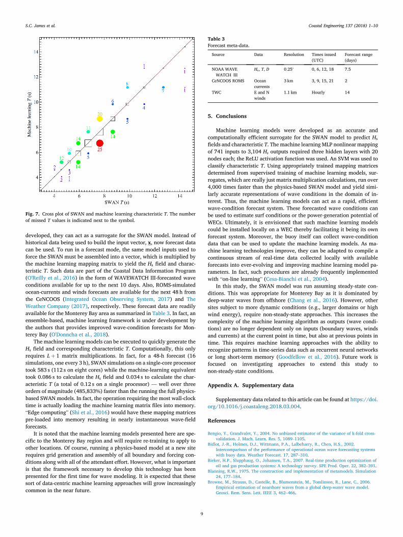
Fig. 7. Cross plot of SWAN and machine learning characteristic T. The numberof missed T values is indicated next to the symbol.

Table 3Forecast meta-data.

Source Data Resolution Times issued(UTC)

Forecast range(days)

NOAA WAVEWATCH III

Hs, T, D 0:25∘ 0, 6, 12, 18 7.5

CeNCOOS ROMS Oceancurrents

3 km 3, 9, 15, 21 2

TWC E and Nwinds

1.1 km Hourly 14

S.C. James et al. Coastal Engineering 137 (2018) 1–10

developed, they can act as a surrogate for the SWAN model. Instead ofhistorical data being used to build the input vector, x, now forecast datacan be used. To run in a forecast mode, the same model inputs used toforce the SWAN must be assembled into a vector, which is multiplied bythe machine learning mapping matrix to yield the Hs field and charac-teristic T. Such data are part of the Coastal Data Information Program(O'Reilly et al., 2016) in the form of WAVEWATCH III-forecasted waveconditions available for up to the next 10 days. Also, ROMS-simulatedocean-currents and winds forecasts are available for the next 48 h fromthe CeNCOOS (Integrated Ocean Observing System, 2017) and TheWeather Company (2017), respectively. These forecast data are readilyavailable for the Monterey Bay area as summarized in Table 3. In fact, anensemble-based, machine learning framework is under development bythe authors that provides improved wave-condition forecasts for Mon-terey Bay (O'Donncha et al., 2018).

The machine learning models can be executed to quickly generate theHs field and corresponding characteristic T. Computationally, this onlyrequires Lþ 1 matrix multiplications. In fact, for a 48-h forecast (16simulations, one every 3 h), SWAN simulations on a single-core processortook 583 s (112 s on eight cores) while the machine-learning equivalenttook 0.086 s to calculate the Hs field and 0.034 s to calculate the char-acteristic T (a total of 0.12 s on a single processor) — well over threeorders of magnitude (485,833%) faster than the running the full physics-based SWAN models. In fact, the operation requiring the most wall-clocktime is actually loading the machine learning matrix files into memory.“Edge computing” (Shi et al., 2016) would have these mapping matricespre-loaded into memory resulting in nearly instantaneous wave-fieldforecasts.

It is noted that the machine learning models presented here are spe-cific to the Monterey Bay region and will require re-training to apply toother locations. Of course, running a physics-based model at a new siterequires grid generation and assembly of all boundary and forcing con-ditions along with all of the attendant effort. However, what is importantis that the framework necessary to develop this technology has beenpresented for the first time for wave modeling. It is expected that thesesort of data-centric machine learning approaches will grow increasinglycommon in the near future.

9

5. Conclusions

Machine learning models were developed as an accurate andcomputationally efficient surrogate for the SWAN model to predict Hs

fields and characteristic T. The machine learningMLP nonlinear mappingof 741 inputs to 3,104 Hs outputs required three hidden layers with 20nodes each; the ReLU activation function was used. An SVM was used toclassify characteristic T. Using appropriately trained mapping matricesdetermined from supervised training of machine learning models, sur-rogates, which are really just matrix multiplication calculations, run over4,000 times faster than the physics-based SWAN model and yield simi-larly accurate representations of wave conditions in the domain of in-terest. Thus, the machine learning models can act as a rapid, efficientwave-condition forecast system. These forecasted wave conditions canbe used to estimate surf conditions or the power-generation potential ofWECs. Ultimately, it is envisioned that such machine learning modelscould be installed locally on a WEC thereby facilitating it being its ownforecast system. Moreover, the buoy itself can collect wave-conditiondata that can be used to update the machine learning models. As ma-chine learning technologies improve, they can be adapted to compile acontinuous stream of real-time data collected locally with availableforecasts into ever-evolving and improving machine learning model pa-rameters. In fact, such procedures are already frequently implementedwith “on-line learning” (Cesa-Bianchi et al., 2004).

In this study, the SWAN model was run assuming steady-state con-ditions. This was appropriate for Monterey Bay as it is dominated bydeep-water waves from offshore (Chang et al., 2016). However, othersites subject to more dynamic conditions (e.g., larger domains or highwind energy), require non-steady-state approaches. This increases thecomplexity of the machine learning algorithm as outputs (wave condi-tions) are no longer dependent only on inputs (boundary waves, windsand currents) at the current point in time, but also at previous points intime. This requires machine learning approaches with the ability torecognize patterns in time-series data such as recurrent neural networksor long short-term memory (Goodfellow et al., 2016). Future work isfocused on investigating approaches to extend this study tonon-steady-state conditions.

Appendix A. Supplementary data

Supplementary data related to this article can be found at https://doi.org/10.1016/j.coastaleng.2018.03.004.

References

Bengio, Y., Grandvalet, Y., 2004. No unbiased estimator of the variance of k-fold cross-validation. J. Mach. Learn. Res. 5, 1089–1105.

Bidlot, J.-R., Holmes, D.J., Wittmann, P.A., Lalbeharry, R., Chen, H.S., 2002.Intercomparison of the performance of operational ocean wave forecasting systemswith buoy data. Weather Forecast. 17, 287–310.

Bieker, H.P., Slupphaug, O., Johansen, T.A., 2007. Real-time production optimization ofoil and gas production systems: A technology survey. SPE Prod. Oper. 22, 382–391.

Blanning, R.W., 1975. The construction and implementation of metamodels. Simulation24, 177–184.

Browne, M., Strauss, D., Castelle, B., Blumenstein, M., Tomlinson, R., Lane, C., 2006.Empirical estimation of nearshore waves from a global deep-water wave model.Geosci. Rem. Sens. Lett. IEEE 3, 462–466.

S.C. James et al. Coastal Engineering 137 (2018) 1–10

Browne, M., Castelle, B., Strauss, D., Tomlinson, R., Blumenstein, M., Lane, C., 2007.Near-shore swell estimation from a global wind-wave model: Spectral process, linear,and artificial neural network models. Coast Eng. 54, 445–460.

Cahill, B., Lewis, T., 2014. Wave period ratios and the calculation of wave power. In:Proceedings of the 2nd Marine Energy Technology Symposium, pp. 1–10.

Cesa-Bianchi, N., Conconi, A., Gentile, C., 2004. On the generalization ability of on-linelearning algorithms. IEEE Trans. Inf. Theor. 50, 2050–2057.

Chang, G., Ruehl, K., Jones, C., Roberts, J.D., Chartrand, C.C., 2016. Numerical modelingof the effects of wave energy converter characteristics on nearshore wave conditions.Renew. Energy 89, 636–648.

DeVries, P.M., Thompson, T.B., Meade, B.J., 2017. Enabling large-scale viscoelasticcalculations via neural network acceleration. Geophys. Res. Lett. 44, 2662–2669.

Dushaw, B.D., Egbert, G.D., Worcester, P.F., Cornuelle, B.D., Howe, B.M., Metzger, K.,1997. A TOPEX/POSEIDON global tidal model (TPXO.2) and barotropic tidalcurrents determined from long-range acoustic transmissions. Prog. Oceanogr. 40,337–367.

EPRI, 2011. Mapping and Assessment of the United States Ocean Wave Energy Resource.Technical Report 1024637, Palo Alto, CA.

Etemad-Shahidi, A., Mahjoobi, J., 2009. Comparison between M5’ model tree and neuralnetworks for prediction of significant wave height in Lake Superior. Ocean Eng. 36,1175–1181.

FAO, 2016. The State of the World Fisheries and Aquaculture 2016. Contributing to theFood Security and Nutrition for All. Technical Report. Food and AgricultureOrganization of the United Nations.

Goodfellow, I., Bengio, Y., Courville, A., 2016. Deep Learning. MIT Press.Haas, K., Ahn, S., Neary, V.S., Bredin, S., 2017. Development of a wave energy resource

classification system. Waterpower Week 1–5.Hodur, R.M., 1997. The Naval Research Laboratory's coupled ocean/atmosphere

mesoscale prediction system (COAMPS). Mon. Weather Rev. 125, 1414–1430.Integrated Ocean Observing System, 2017. Central and Northern California Ocean

Observing System. CeNCOOS.Kingma, D.P., Ba, J., 2014. Adam: A Method for Stochastic Optimization. arXiv preprint

arXiv:1412.6980.Kleijnen, J.P., 2009. Kriging metamodeling in simulation: A review. Eur. J. Oper. Res.

192, 707–716.Knerr, S., Personnaz, L., Dreyfus, G., 1990. Single-layer learning revisited: A stepwise

procedure for building and training a neural network. Neurocomp. NATO ASI Ser.(Ser. F: Comp. Syst. Sci.) 68, 41–50.

Komen, G.J., Cavaleri, L., Donelan, M., 1996. Dynamics and Modelling of Ocean Waves.Cambridge University Press.

LeCun, Y., Bengio, Y., Hinton, G., 2015. Deep learning. Nature 521, 436–444.Mahjoobi, J., Etemad-Shahidi, A., 2008. An alternative approach for the prediction of

significant wave heights based on classification and regression trees. Appl. OceanRes. 30, 172–177.

10

Makarynskyy, O., 2004. Improving wave predictions with artificial neural networks.Ocean Eng. 31, 709–724.

Mallet, V., Stoltz, G., Mauricette, B., 2009. Ozone ensemble forecast with machinelearning algorithms. J. Geophys. Res.: Atmos. 114.

Mei, C.C., Stiassnie, M., Yue, D.K.-P., 1989. Theory and Applications of Ocean SurfaceWaves: Part 1: Linear Aspects. Part 2: Nonlinear Aspects. World Scientific.

Moore, R., DeNero, J., 2011. L1 and L2 regularization for multiclass hinge loss models. In:Symposium on Machine Learning in Speech and Language Processing, pp. 1–5.

Nair, V., Hinton, G.E., 2010. Rectified linear units improve restricted Boltzmannmachines. In: Proceedings of the 27th International Conference on Machine Learning.

Ocean Energy Systems, 2016. Annual Report: Ocean Energy Systems 2016. TechnicalReport 1024637.

O'Donncha, F., Zhang, Y., James, S.C., 2018. An integrated framework that combinesmachine learning and numerical models to improve wave-condition forecasts. J. Mar.Syst.

O'Hagan, A., 2006. Bayesian analysis of computer code outputs: A tutorial. Reliab. Eng.Syst. Saf. 91, 1290–1300.

O'Reilly, W., Olfe, C.B., Thomas, J., Seymour, R., Guza, R., 2016. The California coastalwave monitoring and prediction system. Coast Eng. 116, 118–132.

Patterson, J., Thomas, J., Rosenfeld, L., Newton, J., Hazard, L., Scianna, J., Kudela, R.,Mayorga, E., Cohen, C., Cook, M., et al., 2012. Addressing Ocean and Coastal Issues atthe West Coast Scale through Regional Ocean Observing System Collaboration. MTS/IEEE OCEANS’12, pp. 1–8.

Pedregosa, F., Varoquaux, G., Gramfort, A., Michel, V., Thirion, B., Grisel, O., Blondel, M.,Prettenhofer, P., Weiss, R., Dubourg, V., et al., 2011. SciKit-learn: Machine learningin Python. J. Mach. Learn. Res. 12, 2825–2830.

Peres, D., Iuppa, C., Cavallaro, L., Cancelliere, A., Foti, E., 2015. Significant wave heightrecord extension by neural networks and reanalysis wind data. Ocean Model. 94,128–140.

Razavi, S., Tolson, B.A., Burn, D.H., 2012. Review of surrogate modeling in waterresources. Water Resour. Res. 48. W07401.

Schmidhuber, J., 2015. Deep learning in neural networks: an overview. Neural Network.61, 85–117.

Shi, W. , Cao, J. , Zhang, Q., Li, Y. , Xu, L. , 2016. Edge computing: vision and challenges.IEEE InternetThings J. 3, 637–646.

Song, Y., Haidvogel, D., 1994. A semi-implicit ocean circulation model using ageneralized topography-following coordinate system. J. Comput. Phys. 115,228–244.

The SWAN Team, 2006. SWAN Scientific and Technical Documentation. Technical ReportSWAN Cycle III version 40.51. Delft University of Technology.

The Weather Company, 2017. The Weather Company.Tolman, H.L., et al., 2009. User manual and system documentation of WAVEWATCH IIITM

version 3.14, Technical note. MMAB Contrib. 276, 220.US DOE, 2016. Energy Department Announces Investment in Wave Energy Test Facility.