A Bayesian partial identification approach to inferringthe prevalence of accounting misconduct

P. Richard Hahn∗

Booth School of Business, University of ChicagoJared S. Murray

Department of Statistics, Carnegie Mellon UniversityIoanna Manolopoulou

Department of Statistical Science, University College London

July 21, 2015

Abstract

This paper describes the use of flexible Bayesian regression models for estimatinga partially identified probability function. Our approach permits efficient sensitivityanalysis concerning the posterior impact of priors on the partially identified compo-nent of the regression model. The new methodology is illustrated on an importantproblem where only partially observed data are available – inferring the prevalenceof accounting misconduct among publicly traded U.S. businesses.

Keywords: Bayesian inference, nonlinear regression, partial identification, sampling bias,sensitivity analysis, set identification.

∗The first author thanks Joseph Gerakos for helpful discussions and the Booth School of Business forsupporting this research. The second author was supported in part by the National Science Foundationunder grant numbers SES-11-31897, SES-1130706 and DMS-1043903. Any opinions, findings, and con-clusions or recommendations expressed in this material are those of the author(s) and do not necessarilyreflect the views of the National Science Foundation.

1

1 Introduction

This paper develops an approach for estimating partially identified parameters in nonlinear

regression settings. Our approach is based on a decomposition of the probability function

into an identified and a partially identified component (Kadane, 1975). This representation

permits us to employ flexible (nonlinear) models when inferring the identified component; in

our applications we utilize Bayesian tree-based priors for the regression functions (Chipman

et al., 2010; Hill, 2012). For the partially identified portion of the model, informative

priors are crucial, so checking the sensitivity of posterior inferences to model specification

is vital. In our proposed framework, this sensitivity analysis is straightforward, and may be

conducted under many different models for the partially identified parameters using only

one set of samples from the marginal posterior of the identified parameters.

Our motivating application comes from the corporate accounting literature, where there

is substantial interest in determining what fraction of U.S. firms engage in financial mis-

conduct (such as misstated earnings); e.g. Dyck et al. (2013). Inferring the prevalence of

misconduct is complicated by an inherent partial observability—not all cases of miscon-

duct are discovered. Any treatment of this problem will therefore need to analyze how

company attributes impact the probability of misconduct being discovered in addition to

the probability of the misconduct itself taking place.

As further evidence of the generality of our approach, we also include a reanalysis of a

published dataset (from a broken randomized encouragement study of flu vaccine) in the

supplementary material.

The remainder of this section collects necessary background material, providing an

overview of the concept of partial identification (specifically its treatment from a Bayesian

perspective) and describing the empirical data we will analyze. Section 2 lays out our

2

inferential framework and fixes notation. Section 3 describes the results of our data analysis.

Section 4 concludes with a discussion.

1.1 Partial identification

A statistical model p(y | τ) indexed by a parameter τ ∈ T is said to be identifiable or

identified if parameter values correspond uniquely to distinct probability distributions over

observables. That is, p(y | τ) = p(y | τ ′) for all y if and only if τ = τ ′. A model that

is not identified is simply referred to as unidentified. The importance of identifiability

as a modeling concern has its earliest roots in econometrics, the term first being intro-

duced in Koopmans (1949). Other seminal references include Haavelmo (1943, 1944) and

Koopmans and Reiersol (1950). Unidentifiability arises naturally in econometric analysis

of observational data as a byproduct of imperfect measurement and/or various data cen-

soring mechanisms. The Bayesian perspective on identifiability has been comprehensively

reviewed in Aldrich (2002) and more recently in San Martın and Gonzalez (2010).

The notion of partial identifiability or partial identification of parameters expands the

concept of identification to consider cases of partial learning. A more general definition

of identifiability is p(y | τ) = p(y | τ ′) if and only if t(τ) = t(τ ′) for some non-constant

function t; here t is an “identifying function” in the terminology of Kadane (1975). When t

is one-to-one, we recover the traditional definition of identifiability, or point identification.

When the t with the finest preimage satisfying this condition is many-to-one, the model is

partially identified — the intuition being that asymptotically we can only isolate the value

of t(τ) consistent with the data, which will correspond to a proper subset of T with more

than one element. For this reason, and in contrast to point identification, it is common

to talk of set or partial identification. For a more rigorous exposition of the theory of

functional identification, refer to Kadane (1975).

3

Early examples of the partial identification concept include Frisch (1934), Frechet (1951)

and Duncan and Davis (1953). In recent years, interest in partial identification has acceler-

ated; an excellent recent review article is Tamer (2010) which includes comprehensive cita-

tions. See also the book-length treatments by Manski (Manski, 1995, 2003, 2007). Recent

contributions from a Bayesian perspective have focused primarily on asymptotic properties

of the posterior distribution over partially identified parameters, notably Gustafson (2005)

and Gustafson (2010). Moon and Schorfheide (2012) examine asymptotic discrepancies

between Bayesian credible regions and frequentist confidence sets for set-identified parame-

ters. Florens and Simoni (2011) consider a theoretical framework for studying posteriors of

partially identified parameters in nonparametric models. Kline and Tamer (2013) develop

large sample approximations of posterior probabilities that particular parameter values lie

in the identified set without reference to a prior on the partially identified parameter. See

also the recent book by Gustafson (2015).

Our approach differs from these recent contributions in three ways. One, it is tailored

to a nonlinear regression setting with possibly many predictors and complicated inter-

relationships; most of the recent literature considers much simpler examples, often without

any covariates. Two, our focus is on practical methods for making inferences on parameters

of interest with finite samples; most of the recent literature has focused on theoretical and

specifically large-sample issues. Three, we introduce an efficient computational scheme for

sensitivity analysis, an issue which has received relatively little attention in the literature.

Most previous work focuses on wholly unidentified parameters and typically requires mul-

tiple iterations of model fitting; see e.g. McCandless et al. (2007); Molitor et al. (2009) and

McCandless et al. (2012) in the context of causal inference/observational data analysis, and

Daniels and Hogan (2008) and chapter 15 of Little and Rubin (2002) for extensive reviews

in missing data problems.

4

1.2 Application: inferring the prevalence of accounting miscon-

duct

Since 1982, the United States Securities and Exchange Commission (SEC) has released pub-

lic notices called Accounting and Auditing Enforcement Releases, or AAERs. AAERs are

financial reports “related to enforcement actions concerning civil lawsuits brought by the

Commission in federal court and notices and orders concerning the institution and/or set-

tlement of administrative proceedings” (Securities and Exchange Commission, Accounting

and Auditing Enforcement Releases, 2014). Informally, AAERs comprise a list of publicly

traded firms that the SEC has cited for misconduct in one form or another.

For brevity, we adopt the nomenclature “cheating” and “caught”, with the understand-

ing that “cheating” is operationally defined as any accounting anomaly that would lead to

an AAER being issued, were it explicitly brought to the SEC’s attention. This interpreta-

tion entails that all caught firms are, by definition, “cheaters”.

Our goal is to provide an estimate of the prevalence of accounting misconduct in the U.S.

economy, defined as all actual (caught) and potential (uncaught) AAERs. Predicting which

companies are likely to cheat, on the basis of observable firm characteristics, is complicated

by the fact that there are potentially many instances of misconduct of which the SEC

is unaware. Thus, we do not directly observe which firms cheat, but merely the subset

of cheating firms that were caught doing so. A naive regression analysis would therefore

only speak to the question of which attributes are predictive of getting caught cheating.

To complete the analysis, one must incorporate knowledge or conjectures concerning the

impact firm attributes have on the likelihood of misconduct being discovered.

Problems with a similar structure to the SEC data appear in the literature under the

heading of “partially observed binary data”. Regression models for such data have been

5

studied in many different fields, going by various names. For example, Lancaster and

Imbens (1996) considers the case where the observation model is covariate independent

under the name “contaminated case-control”, building on Prentice and Pyke (1979). Poirier

(1980) studies such data under the rubric of “partially observed bivariate probit models”,

building on the work of Heckman (1976, 1978, 1979). Our analysis is similar to the approach

taken in Wang (2013), which adapts the bivariate probit model of Poirier (1980) for the

securities fraud problem.

Whereas these earlier references considered particular parametric models, such as the

probit model, and studied identification conditions in that setting, we proceed in the more

generic setting of nonlinear regression models, which leads to partially identified parame-

ters. Our approach will be to confront this partial identification with informative priors.

2 Prior specification for partially identified regression

models

As in Dawid (1979); Gelfand and Sahu (1999) and Gustafson (2005), we will work with

a reparameterization of τ into an identified component φ and an unidentified component

(θ, η). We separate the unidentified component into θ, which appears in our estimand of

interest, and η, which collects hyper parameters. We will be interested in the case where φ

and θ are functions of a fixed vector of covariates x. Therefore, we will refer to φ, φ(x) or

φx (respectively, θ, θ(x) or θx) depending on context. We will use φ when the dependence

on x is inessential, we will use φ(x) to emphasize that φ is a function of x, and we will use

φx to refer to point-wise evaluations of φ(x). One may allow η to be a function of x as

well, but we do not explore this possibility here.

The joint distribution over data and parameters in a partially identified model can be

6

written as

π(η, θ, φ, y) = f(y | η, θ, φ)π(η, θ, φ),

= f(y | φ)π(η, θ, φ),

= f(y | φ)π(φ)π(η, θ | φ),

where the conditional independence implied in moving from the first line to the second

line constitutes a definition of partial identification. It follows that the joint posterior

distribution of the identified component φ and the unidentified component (θ, η) can be

written as

π(η, θ, φ | y) =f(y | φ)π(φ)π(η, θ | φ)

f(y)

=f(y | φ)π(φ)

f(y)π(η, θ | φ)

= π(φ | y)π(η, θ | φ).

(1)

Theorem 5 of Kadane (1975) shows rigorously that the parameter space of any model can

be decomposed in this way. Essentially, there are three cases to consider. If the model is

fully identified, then (η, θ) is simply a constant random variable. When the model has fully

unidentified elements, the support of π(η, θ | φ) does not depend on φ; the data inform

about (η, θ) only via the presumed prior dependence represented in the choice of π(η, θ | φ).

In the partially identified case, which we focus on here, π(θ | φ, η) has support restrictions

that do depend on φ; we will denote this restricted support by Ω(φ, η).

Our approach will be to directly specify π(θ | φ, η) with support Ω(φ, η). In principle,

η can be integrated out a priori, but η often proves useful as a device for parameterizing

the conditional prior for θ, in conjunction with a possibly φ-dependent prior π(η | φ). Our

SEC analysis specifies π(η | φ) with non-trivial support restrictions depending on φ, while

in the flu analysis in the supplement we take π(η | φ) = π(η). Algorithmic details are

7

given in section A.1. See Gustafson (2005, 2010) and Florens and Simoni (2011) for similar

decompositions.

More specifically, partial identification arises in our applied analysis due to partially

observed multivariate binary data. The complete data consist of binary vectors U =

(U1, . . . Uk), of which only certain subsets are simultaneously observable. Interest is in

some functional p(x) of the entire joint distribution p(U1, . . . Uk | x), where x denotes a

vector of fixed covariates. Due to the partial observability, p(x) must be reconstructed

from an identified function φ(x) and an unidentified function θ(x).

2.1 A Gaussian process model for the partially identified regres-

sion

Furnishing prior information regarding θ(x) in a predictor-dependent manner strongly mo-

tivates the use of simple parametric models. For starters, consider the construction

F−1θ(x) = h(x)β, (2)

where F−1 is a link function and h denotes some transformation or subset of the covariate

vector. In this case η ≡ β, and a prior over θ(x) is induced by the prior π(β | φ). A chief

difficulty with this type of specification is that nonlinear (possibly discontinuous) regression

models for φ(x) impose complex support restrictions on π(β | φ) — indeed, some samples

from the posterior for φ(x) may contradict the model for θ(x) entirely, meaning that they

imply a set of bounds for θ(x) such that no feasible β exists.

To address this problem, we expand the prior over θ(x) to acknowledge that (2) is only

a guess as to the form of the regression function. Specifically, we center our model for θ(x)

at (2) by assuming that

F−1θ(x) | φ(x), η ∼ GP (h(x)β,ΣX ) 1[θ(x) ∈ Ωφ(x), η] (3)

8

for all x ∈ X . Here GP(m,ΣX ) denotes a Gaussian process kernel with mean m and

covariance ΣX and the indicator function denotes that our prior is truncated to be supported

on Ωφ(x), η.

Additionally, we will assume that (3) is supported on the discrete set of observed data

points, i.e. X = xini=1, (though additional design points of interest could be included

as well). The assumption of a discrete support yields computations involving a truncated

multivariate normal prior, conditional on β. Note that in this specification, β may be given

a proper prior distribution, which may depend on φ(x), or may be fixed at predetermined

values. In our empirical analysis, we assume diagonal covariance functions, which we denote

as ΣX = σ2I. Under this specification, sampling from (θx | η, φx) reduces to drawing

samples from independent truncated univariate normal distributions.

Note that choosing a multivariate normal prior over β, with covariance Σβ, implies a

Gaussian process prior on θ (marginalizing over β) with non-diagonal covariance h(x)TΣβh(x)+

σ2I. This representation can be exploited to approximate Gaussian process priors with

general covariance functions, without requiring onerous draws from multivariate truncated

normal distributions (Pakman and Paninski, 2014). However, we do not explore this pos-

sibility further here.

2.2 Illustration

It is instructive to observe graphically how the approach works in a simple problem where

the predictor variable x is one-dimensional. Therefore, consider the following definitions of

φ(x) and θ(x) for x ∈ [0, 1]:

φ(x) = 0.05 + 0.7 logistic(14 (x− 0.5)),

θ(x) = 0.1 + 0.7 logistic(16 (x− 0.5) + 50 (x− 0.5)2)

9

These formulae are included for replicability, but the set-up is easiest to see graphically as

illustrated in Figure 1a. The important features are that φ(x) and θ(x) both lie between

0 and 1 and φ(x) ≤ θ(x) for all values of x ∈ [0, 1]. Suppose that i = 1, . . . , n = 100 data

pairs (xi, yi) are observed, with Pr(Yi = 1 | Xi = x) = φ(x), and suppose that interest is

in the ratio p(x) ≡ φ(x)θ(x)

. Clearly p(x) is unidentified through its dependence on θ alone.

Nonetheless, the data do inform us about possible values of θ(x), and hence p(x), due to

the constraint that φ(x) ≤ θ(x). That is, in this example Ωφ(x), η = θ(x) | φ(x) ≤

θ(x) ≤ 1 ∀x ∈ X (no hyperparameter η has been designated yet).

We specify a prior on θ(x) as

Φ−1(θ(x)) ∼ GP(β0 + β1x+ β2x

2, σ2I)1[θ(x) ∈ Ωφ(x), η]

where Φ(·) is the standard normal inverse cumulative distribution function. We fix β0 =

1, β1 = −9, β2 = 9, to mimic the elicitation of a “U-shaped” regression function. In the

notation of section 2, we have h(x) = (1, x, x2) and β = (1,−9, 9)T .

As seen in Figure 1a, this prior guess is grossly incorrect. However, in regions where

the data are uninformative via the bounds supplied by φ(x), the prior happens to be close

to the truth. Therefore, this prior, coupled with the observed data, yields a reasonably

accurate estimate of θ(x) and of p(x) (Fig. 2a, left) in the sense that the posterior 95%

credible interval of α ≡ n−1∑

i φ(xi)/θ(xi) contains the true value (Fig. 2a, right). The

raw estimate from the data, i.e., assuming θ(x) = 1 for all x, would have given the much

smaller estimate of approximately 1/2. Of course, this is an ideal scenario — the prior for θ

is correct where the data are uninformative, and the data are fairly informative — through

Ωφ(x), η— where the prior for θ is incorrect. In general we will have no such assurances,

so it is important that the modular prior is carefully chosen and that the sensitivity of

posterior inference to multiple specifications of the modular prior is assessed. In appendix

10

B we consider other, less fortuitous choices of prior distributions.

It is possible to further improve our estimate by supplying additional prior information.

Assume that we believe φ(x)/θ(x) < c for all x, which implies that φ(x)/c ≤ θ(x). Taking

c < 1 defines a larger lower bound on θ(x) than the necessary one, which implicitly takes

c = 1. To connect this specification with the more abstract formulation of section 2, we

have η ≡ c and Ωφ(x), η = θ(x) | φ(x)/c ≤ θ(x) ≤ 1.

Note that the relationship between φ, θ and c also implies that c ≥ supX φ(x). Hence

the data are partially informative about c as well, and may contradict any particular fixed

value. So rather than fixing c to some value c0 we assign it a proper prior, concentrated

around c0 and truncated to the appropriate region, with a scale parameter controlling the

degree of prior belief in c0. For this example we assign c a Beta(vc0, v(1− c0)) distribution,

truncated to have support c ≥ supX φ(x). Here we take c0 = 0.65 and v = 100, considering

other specifications in appendix B.

The results under this more informative prior are shown in Figures 1b and 2b. Because

the true parameter values satisfy φ(xi)/θ(xi) < 0.8 across all i, the chosen prior on c induces

a prior on θ(x) which proves beneficial. Different choices of m(x) and prior over c yield

different posterior estimates; Appendix B explores additional specifications.

3 Analysis of AAER data, 2004-2010

Let Zi indicate “cheating” in firm-year i, let Wi indicate “getting caught” in firm-year i,

(U1 = W and U2 = Z) and let x denote a vector of firm attributes (some which vary by

year, such as income, and others that are constant across years, such as industry). We

assume that with some probability, cheaters get caught, but that there are no firms who

get caught when they are not cheating (this is consistent with our operational definition of

11

0.0 0.2 0.4 0.6 0.8 1.0

0.0

0.2

0.4

0.6

0.8

1.0

x

Pro

babi

lity

(a)

0.0 0.2 0.4 0.6 0.8 1.0

0.0

0.2

0.4

0.6

0.8

1.0

x

Pro

babi

lity

(b)

Figure 1: (a) The thin solid line indicates φ(x); the bold solid line indicates the true θ(x);

the dashed line indicates the point prior mean for θ(x); the dotted line depicts a single draw

from the BART posterior for φ(x). The filled circles indicate draws from the posterior on

θ(x); note that they obey the lower truncation imposed by the dotted line. (b) Giving c

a Beta(100c0, 100(1 − c0)) prior with c0 = 0.65, posterior draws of θ(x) (black dots) are

observed to be further away from the lower bound φ(x) (dotted line) in regions where θ(x)’s

prior mean, m(x) (dashed line), is much less than φ(x). Compare to Figure 1a, where the

posterior draws of θ(x) hug the lower bound tightly.

12

0.0 0.2 0.4 0.6 0.8 1.0

0.2

0.4

0.6

0.8

x

Probability

0.55 0.60 0.65 0.70 0.75 0.80 0.85

02

46

8

α

Density

(a)

0.0 0.2 0.4 0.6 0.8 1.0

0.0

0.2

0.4

0.6

0.8

1.0

x

Probability

0.4 0.5 0.6 0.7 0.8 0.90

12

34

56

α

Density

(b)

Figure 2: (a) (left) Posterior mean (solid gray) and 90% credible interval for θ(x) (shaded),

along with its prior mean (dashed) and true value (solid black). Because the prior matches

the truth in regions where the data is uninformative and is incorrect in regions where the

data is informative, the posterior mean ends up relatively close to the truth. (Right) A

posterior density (smoothed) for α ≡ n−1∑

i φ(xi)/θ(xi). Because the posterior for θ(x)

well-approximates the truth, a decent estimate of the true value of α (shown as a dashed

vertical line) is achieved. (b) Providing prior bias that φ(x)/θ(x) < c0 = 0.65 leads to

improved estimation of both φ(xi)/θ(xi) (at left, solid gray is posterior mean, solid black

is true, dashed is prior mean) and α ≡ n−1∑

i φ(xi)/θ(xi) (at right, truth is shown by the

vertical dashed line) .

13

“cheating”). Additionally, the data are “presence-only” in that we have no confirmation

that any given firm is certainly non-cheating.

The parameter of interest is the marginal firm-year probability of cheating,

p(x) = Pr(Z = 1 | x) =Pr(W = 1, Z = 1 | x)

Pr(W = 1 | Z = 1, x)

from which we may determine the overall prevalence of cheating across all firms as

α ≡ n−1n∑i=1

Pr(Zi = 1 | xi) = n−1∑i

Pr(Zi = 1,Wi = 1 | xi)Pr(Wi = 1 | Zi = 1, xi)

. (4)

Equivalently, for each firm-year we observe Yi ≡ ZiWi instead of (Zi,Wi), where Yi

indicating whether a firm received an AAER (cheated and got caught), giving

φ(x) = Pr(Z = 1,W = 1 | x) = Pr(Y = 1 | x); θ(x) = Pr(W = 1 | Z = 1, x).

As φ(x) is simply the (conditional) probability of the observed binary data Y , it is

point identified. In our application, we estimate φ(x) using the BART model described

in the Appendix. BART has been shown empirically to be an excellent default nonlinear

regression method, with a demonstrated ability to handle many noise variables and strong

nonlinearities (Chipman et al., 2010; Hill, 2012).

The partial identification of p(x) arises simply because 0 ≤ p(x) ≤ 1. Given φ(x), the

posterior on p(x) is defined by the prior over θ(x), truncated to regions satisfying

0 ≤ φ(x)

θ(x)≤ 1, (5)

for all x ∈ X . In other words, in our applied setting, Ωφ(x), η = θ(x) | φ(x) ≤ θ(x), ∀x ∈

X, just as in our example from section 2.2.

14

3.1 Data

Our data are aggregated from three main sources. First, the AAER response variable was

obtained from the Center for Financial Reporting and Management (CFRM) at Berkeley’s

Haas School of Business. Detailed information about the full data set can be found in

Dechow et al. (2011).

Second, additional firm attributes are obtained from the CompuStat North America

Annual Fundamentals database via the Wharton Research Data Service (WRDS). These

data are then merged with the AAERs using Global Company Key (GVKEY) by year.

Specifically, the covariate vector x consists of:

• fiscal year,

• cash,

• net income,

• capital investments,

• SIC industry code,

• qui tam dummy variable.

Cash, net income and capital investments are all recorded as a fraction of the firm’s total

assets. Standard industrial classifications are given in terms of ten major divisions, denoted

A-J by the Occupational Safety and Health Administration. The qui tam dummy variable is

derived from the SIC codes; it denotes if a firm is in an industry where persons responsible

for revealing misconduct are eligible to receive some part of any award resulting from

subsequent prosecution. Similar to Dyck et al. (2008) and Jayaraman and Milbourn (2010),

our qui tam variable is set to one for firms with SIC code 381x, 283x, 37xx, 5122 or 80xx,

which includes healthcare providers and pharmaceutical firms, and airplane, missile, and

tank manufacturers. It is reasonable to suppose that firms in these industries have a greater

likelihood of any misconduct being exposed as a result of incentivized employees.

15

Finally, a keyword search at the Financial Times web page (www.ft.com) was conducted

on each company name and the number of search results was recorded by year. This variable

provides a crude measure of media exposure. Although discrepancies between firm names

as recorded in CompuStat and firm names as reported in Financial Times articles lead to

measurement error of this variable, it still provides a reasonable proxy for name recognition

and cultural visibility. Most firms will never be mentioned in any news article; a few firms

are routinely mentioned in the press. To adjust for the fact that web traffic has increased

over that period, we normalize the search results count by the total number of hits across

all companies in a given year.

We restrict our analysis to U.S. firms that had positive net income for the given year,

considering the period between 2004 and 2010, for a total of 6, 641 unique firms and a total

of n = 25, 889 total firm-year observations.

3.2 Surveillance model

The unidentified function θ(x) can be thought of as a “surveillance” probability; it encodes

which attributes invite (discourage) SEC scrutiny, making cheaters more (less) likely to

be caught. Its effect is to inflate the probability of cheating, which is intuitive since the

proportion of caught cheaters φ(x) represents an obvious lower bound on the proportion of

actual cheaters.

Our surveillance model takes the form reported in expression (3) with ΣX = σ2I and

using a logit link. We scale and shift all variables to reside on the unit interval, taking

shifted log transformations of the financial times search hits and net income. We chose to

place nonzero coefficients on the (fiscal) year of misconduct, media exposure (as measured

by Financial Times search hits), income, cash, and a dummy for qui tam industries. We

have specific reasons to expect that these variables are important determinants of the

16

2004 2005 2006 2007 2008 2009 2010

Fiscal year

AA

ER

rate

1%2%

Figure 3: AAERs are more common in earlier years, likely because they may be filed

retroactively, not because cheating was more prevalent in the past.

surveillance probability, allowing us to chose informative values for β.

First, note that the frequency of AAERs is substantially higher in earlier years; see

Figure 3. AAERs may be filed retroactively, so the opportunity to discover and report

misconduct in a given year increases over time. Fitting a curve to the data in Figure 3

suggests a coefficient of roughly βfyear = −2.5. Observe that this makes the posterior

probability of cheating approximately constant across the years examined, which seems

plausible.

Second, it is reasonable to assume that media attention naturally draws SEC scrutiny

(Miller, 2006). The SEC has a vested interest in catching and making examples of any

high-profile cheaters. We set βFThits = 2, implying approximately a six-fold difference in

the probability of misconduct being discovered between a company with no media exposure

and the company with the highest media exposure. Similarly, we set βquitam = 1, implying

approximately a two-fold increase in misconduct being discovered for companies in qui

tam industries where employees are incentivized to report misconduct. These observations

constitute the subjective information contained in our first observation model A.

To determine the intercept term, consider the following argument: AAERs are quite

17

Intercept Fiscal year FT.com hits cash net income qui tam

βA 0 −2.5 2 0 0 1

βB −0.85 −2.5 2 −1.50 2.5 1

Table 1: Regression coefficients defining surveillance models A and B. They differ in their

intercept terms and their cash and net income coefficients. The intercepts have been

adjusted to obtain an average misconduct discovery rate of 30%

rare, with an observed aggregate incidence in our sample of only 0.5%. Potentially this

is because very few firms exhibit actionable misconduct, but more likely it is because the

SEC has limited resources to identify and pursue violations. Accordingly, one sensible

calibration method would be fix the mean probability of discovery across all firms. Fixing

this quantity and the other elements of β, we may then solve for the intercept β0. In the

case of model A, fixing the average discovery rate to 30% gives β0 = 0.

After obtaining posterior samples under model A, we observe that cash appears to have

a negative impact on the probability of cheating. In contrast, net income appears to have a

positive impact on the probability of cheating. We might surmise that these trends are due

to unadjusted surveillance probabilities. For example, one could argue that having large

amounts of cash on hand (relative to total assets) provides a measure of “wiggle room”

that makes certain kinds of misconduct harder to discover. Likewise, firms with high

income are more likely to draw SEC attention than firms with smaller income streams. To

compare our results under these narratives, we specify a second surveillance model (B),

with βcash = −1.5 and βincome = 2.5. Setting the intercept for model B to match the

30% discovery rate of model A gives β0 = −0.85. Surveillance models A and B are shown

side-by-side in Table 1.

18

3.2.1 Upper bounding firm-year cheating probability

Finally, we introduce an additional parameter c that allows us to interject prior information

concerning an upper bound on the probability of cheating, as was done in the example

of section 2.2. Recall that the partial identification in this application is driven by the

inequality Pr(Z = 1 | x) = φ(x)/θ(x) ≤ 1, which implies φ(x) ≤ θ(x); the left hand

side of this latter inequality is identified by the data. Extremely high probabilities of

cheating are implausible, motivating us to consider alternative truncations: Pr(Z = 1 |

x) = φ(x)/θ(x) ≤ c, which implies φ(x)/c ≤ θ(x) and c ≥ φ(x) for all x. In terms of the

notation in section 2, we have η ≡ c and Ωφ(x), η = θ(x) | φ(x)/c ≤ θ(x) ≤ 1 ∀x ∈ X.

As in our example in section 2.2, φ(x) is identified so the data may contradict any particular

value of c.

We specify π(c | φ(x)) ∝ Beta (10c0, 10(1− c0)) 1c ≥ supX φ(x) so that c0 captures

prior beliefs about the upper bound on Pr(Z = 1 | x), the probability of cheating for any

firm. Our prior for (θx | c, φX) again takes the form in expression (3), with various fixed

specifications of β and h(x) as described above, and Ωφ(x), η = θ(x) | φ(x)/c ≤ θ(x) ≤

1 ∀x ∈ X. The covariance is taken as σ2I, with both σ2 and c0 subject to a range of

specifications for sensitivity analysis in the following subsection.

Our surveillance models allow us to include prior information in the form of subject

matter knowledge about the impact of various covariates. We are also able to include

additional subjective prior information about α ≡ n−1∑

i Pr(Wi = 1 | Zi = 1, xi) — the

overall prevalence, i.e., average probability, of a cheating firm getting caught — via the

intercept terms, and maxiPr(Zi = 1 | xi) — an upper probability on any firm cheating —

via the prior on c. Computational details are included in the Appendix.

19

3.3 Results

We conduct a sensitivity analysis by varying the parameters σ and c0 for both model

coefficients βA and βB above. Specifically, we consider two settings of each (σ ∈ 0.25, 0.5

and c0 ∈ 0.4, 0.8) for a total of eight candidate models. We study the impact these

choices have on both Pr(Z = 1 | x) as a function of individual predictor variables, and also

on the overall misconduct prevalence α.

Figure 4 shows the posterior distribution of the adjusted cheating prevalence under the

different models. As can be seen in the top panel, increasing σ or c0 alone has little effect on

the overall adjusted cheating prevalence. These two parameters control different aspects of

the surveillance uncertainty: a high c0 implies that any probability of cheating is plausible,

whereas a high σ allows large deviations from the specified surveillance model logistic term.

Under these values of c0 and σ, we observe that the prevalence of misconduct is inferred to

be less than 15% with high probability.

The bottom panel of Figure 4 shows the posterior prevalence for each different SIC

code under the two priors, fixing (σ = 0.25, c0 = 0.4). Under both priors, SIC category

D, representing “electricity, gas, steam and air conditioning supply”, shows much lower

cheating prevalence than categories (B,E,H), which correspond to “mining and quarrying”,

“water supply, sewerage, waste management and remediation activities”, and “transporta-

tion and storage” respectively. This finding squares with prior expectation that misconduct

prevalence should vary by industry.

Because BART is nonlinear, summary plots of the impact of individual covariates are

challenging to visualize, even if the surveillance model is relatively simple, such as our

linear logistic specification. It is instructive, therefore, to examine the implied probability

of cheating as one varies individual covariates, for a given firm. That is, how does Pr(Z =

1 | x) change as a function of xj while holding x−j fixed?

20

Raw (0.25,0.4) (0.5,0.4) (0.25,0.8) (0.5,0.8) (0.25,0.4) (0.5,0.4) (0.25,0.8) (0.5,0.8)

0.00

0.05

0.10

0.15

0.00

0.05

0.10

0.15

0.20

0.25

SIC category

A B C D E F G H I J

Figure 4: Top panel: posterior cheating prevalence, white corresponding to the raw (un-

adjusted) prevalence, pink to prior A and blue to prior B. The four boxplots within

each prior correspond to the following combinations for c and σ (from left to right):

(σ = 0.25, c0 = 0.4), (σ = 0.25, c0 = 0.8), (σ = 0.5, c0 = 0.4), (σ = 0.5, c0 = 0.8).

Bottom panel: Posterior cheating prevalence in companies within each SIC code, pink

corresponding to prior A and blue to prior B for (σ = 0.25, c0 = 0.4).

21

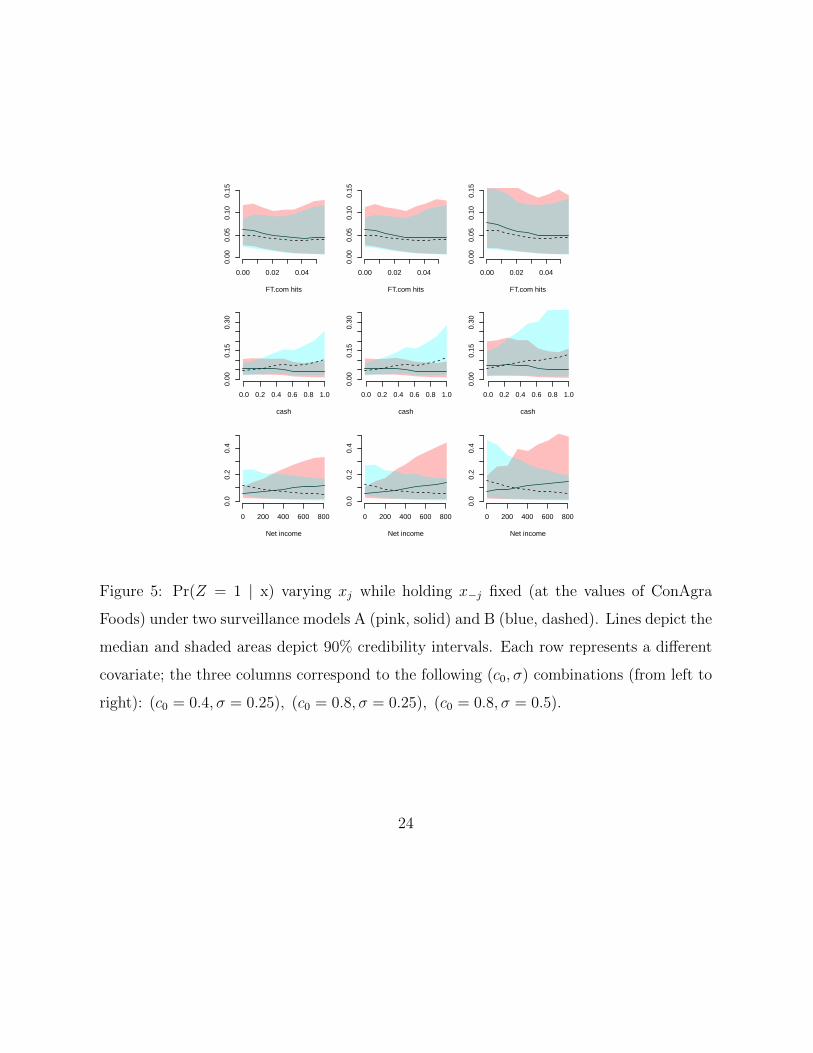
To demonstrate this approach, we focus on a specific firm, ConAgra Foods of Omaha,

Nebraska (simply because it yields illustrative plots). Figure 5 shows Pr(Z = 1 | x), varying

media attention, cash, and net income under priors A and B and for various combinations

of c0 and σ. As expected, the surveillance model coefficients on cash and net income reverse

the associated slope of the probability of cheating. High values of both σ and c0 results

in posterior credible intervals of up to 40% probability of cheating for some values of net

income.

We have reported here only a small number of the possible variations one would pre-

sumably want to investigate; we make no claims that models A and B are ideal or even

necessarily good or realistic models. Rather, our sensitivity analysis demonstrates a range

of possible comparisons that one might undertake when investigating how various assump-

tions interact with the data via the identified portion of the model.

An important upshot of our analysis is that the surveillance model intercept terms—

which govern the average probability of misconduct discovery (getting caught) across firm—

and the parameter c— which defines the upper bound Pr(Zi = 1 | xi) ≤ c for all i — play

dominant roles in determining the inferred overall prevalence of misconduct. For our choices

of 30% misconduct discovery probability and c0 = 0.4 or 0.8, we find that no more than

15% of firms engage in accounting misconduct.

This finding is consistent with that of Dyck et al. (2013), who put the prevalence at

between 4.74% to 15%, based on a clever natural experiment resulting from the dissolution

of the large accounting firm Arthur Andersen and the subsequent re-audit of its clients

following the Enron scandal. Unavailability of their exact data, as well as the unavailability

of the data of Wang (2013) at the time of writing, means that we cannot compare their

precise estimates with those from our model. However, our partial identification analysis

suggests that any similar analysis is likely to yield similar conclusions in the matter of

22

overall prevalence. After all, there is only so much information in the available data, with

the rest coming from auxiliary assumptions about the surveillance probability, whether

those assumptions are explicit, as in our model, implicit, as in the joint likelihood assumed

by Wang (2013), or based on supplementary evidence, as in Dyck et al. (2013). To the

extent that these various approaches supply similar assumptions, they will yield similar

conclusions. Our approach, by layering such assumptions over the data ex post, permits

systematic sensitivity analysis rather than one-off comparisons of published studies whose

authors are committed to one particular approach.

4 Discussion

We conclude by comparing our modular prior approach to that of Wang (2013), which

similarly attempts to infer the prevalence of fraud using the SEC data, on a simulated data

set. This comparison serves to further highlight the advantages of our approach relative

to parametric alternatives in problems exhibiting partial identification. We consider the

performance of our approach relative to a correctly specified parametric model and also to

a misspecified parametric model.

Wang (2013) builds off Poirier (1980), which considers a latent Gaussian utility formu-

lation of the bivariate probit model:Z∗

W ∗

∼ N(µ(x),Cρ) (6)

where µ(x) = (γ0 + xTγ, δ0 + xT δ) and Cρ is a 2-by-2 correlation matrix with correlation

parameter ρ. The latent utilities (Z∗,W ∗) give rise to bivariate variables Z ≡ 1(Z∗ > 0) and

W ≡ 1(W ∗ > 0). Poirier (1980) establishes that (subject to certain exclusion restrictions)

the parameters of the model (γ, δ and the correlation parameter ρ) are identified even if

23

0.00 0.02 0.04

0.00

0.05

0.10

0.15

FT.com hits

0.00 0.02 0.04

0.00

0.05

0.10

0.15

FT.com hits

0.00 0.02 0.04

0.00

0.05

0.10

0.15

FT.com hits

0.0 0.2 0.4 0.6 0.8 1.0

0.00

0.15

0.30

cash

0.0 0.2 0.4 0.6 0.8 1.0

0.00

0.15

0.30

cash

0.0 0.2 0.4 0.6 0.8 1.0

0.00

0.15

0.30

cash

0 200 400 600 800

0.0

0.2

0.4

Net income

0 200 400 600 800

0.0

0.2

0.4

Net income

0 200 400 600 800

0.0

0.2

0.4

Net income

Figure 5: Pr(Z = 1 | x) varying xj while holding x−j fixed (at the values of ConAgra

Foods) under two surveillance models A (pink, solid) and B (blue, dashed). Lines depict the

median and shaded areas depict 90% credibility intervals. Each row represents a different

covariate; the three columns correspond to the following (c0, σ) combinations (from left to

right): (c0 = 0.4, σ = 0.25), (c0 = 0.8, σ = 0.25), (c0 = 0.8, σ = 0.5).

24

only Y ≡ ZW is observed. Wang (2013) proposes to leverage this result, while deviating

from the latent utility formulation. In particular, despite making a “no false positives”

assumption (as we did in our analysis), Wang (2013) continues to equate Pr(Z∗ > 0 | x)

with the probability of cheating which corresponds to the somewhat arbitrary model:

Pr(cheat, caught) = Φ(γ0 + xTγ, δ0 + xT δ, ρ)

Pr(cheat, not caught) = Φ(γ0 + xTγ)− Φ(γ0 + xTγ, δ0 + xT δ, ρ)

Pr(not cheat, caught) = 0

Pr(not cheat, not caught) = 1− Φ(γ0 + xTγ).

(7)

In other words, Wang (2013) identifies γ from the first equation above, invoking the result

of Poirier (1980), and then proceeds to interpret γ as the parameter from a bivariate probit

model without the no false positives assumption. While there is nothing formally wrong

with this model, its peculiar form appears not well motivated.

All the same, if (7) is in fact the correct model, it is instructive to observe what our

approach gives up to it. Conversely, if (7) is used in a misspecified setting, how do its

results compare to ours? To investigate, we simulated n = 2000 observations from the

following two models. First, we generated data according to (7) by drawing Y ≡ WZ

with (W,Z) coming from a bivariate probit model with γ0 = δ0 = −1/2, γ = (−1, 3/4, 0),

δ = (−3/4, 0,−1/2), and ρ = 1/2, with x1 drawn from a Uniform(−π/2, π/2) distribution,

and x2 and x3 drawn from a Uniform(−3π/2, 3π/2) distribution (independently). This

specification of γ and β satisfies the exclusion restriction of Poirier (1980), in that distinct

predictor variables are omitted from each linear equation in the probit mean function.

A Bayesian specification of Wang (2013), with vague conjugate priors for β and γ

and a uniform prior on (−1, 1) for ρ, was fit using a Gibbs sampler algorithm with a

Metropolis-Hastings update for ρ. Our modular prior approach proceeds by fitting the

25

BART model (with default priors as described in Chipman et al. (2010)) to the observed

data (Yi, xi) and constructing the posterior estimate of Pr(Zi | xi) by dividing posterior

samples of φx by draws of θx from (3), with diagonal covariance σ2I with σ = 0.1 and

mean function set to match the true Pr(W = 1 | Z = 1) implied by (7), i.e. m(x) =

Φ(γ0 + xTγ, δ0 + xT δ, ρ)/

Φ(γ0 + xTγ) . Note that in this case we deviate from our previous

linear specification, m(x) = h(x)β, because we wish to center our prior at the corresponding

probability function from Wang (2013). As in our applied analysis, we have Ωφ(x), η =

θ(x) | φ(x) ≤ θ(x), ∀x ∈ X.

The results are depicted in Figure 6a. As expected, the Wang (2013) model, which

achieves point-identification when it is correctly specified, yields much more accurate infer-

ence compared to our approach. Meanwhile, even with a correct surveillance model in this

case, there persists a modicum of unresolved uncertainty, which reflects that in our model

the estimand is only partially identified. Additionally, we see the impact of the BART prior

pulling the estimated probabilities towards 1/2 in regions near the edges where there are

fewer data points.

To demonstrate how inferences are impacted when the linear probit model is misspeci-

fied, we choose µ(x) = (0.5 + sin (x + π)Tγ, sin (x)T δ) for the above values of γ and δ. The

Wang (2013) model is fit using the unadjusted linear predictors. The modular prior ap-

proach is fit the same as above, but centering (using 3) at the correctly specified surveillance

model: m(x) = Φ(0.5 + sin (x + π)Tγ, sin (x)T δ, ρ)/

Φ(0.5 + sin (x + π)Tγ) .

These results are depicted in Figure 6a. As might be expected, under misspecification

the Wang (2013) model badly mis-estimates the true Pr(Zi = 1 | xi). Our approach, with

good prior information, still does not achieve point identification, but manages to avoid the

gross mis-fit of the Wang (2013) model by successfully recovering the nonlinear identified

component from the data.

26

-4 -2 0 2 4

-4-2

02

4

True cheat z-score

Est

imat

ed c

heat

z-s

core

(a)

-1.0 -0.5 0.0 0.5 1.0 1.5 2.0

-1.0

-0.5

0.0

0.5

1.0

1.5

2.0

True cheat z-score

Est

imat

ed c

heat

z-s

core

(b)

Figure 6: (a) Estimated probability of cheating versus the actual probability of cheating

on the normal linear predictor scale for each of n = 2000 data points. Black solid dots

show the modular prior approach, which loosely surrounds the diagonal, demonstrating

the unresolved uncertainty in the partial identification approach. The solid gray dots

correspond to the Wang (2013) model, which is correctly specified in this example; they

hew more tightly to the diagonal. (b) Estimated probability of cheating versus the actual

probability of cheat on the normal linear predictor scale for each of n = 2000 data points.

Black solid dots show the modular prior approach, which loosely surrounds the diagonal,

demonstrating the unresolved uncertainty in the partial identification approach. The solid

gray dots correspond to the Wang (2013) model, which is incorrectly specified in this

example; they grossly diverge from the diagonal.

27

Naturally, if we had supplied invalid surveillance models, our approach may have been

far off the mark in both cases. The point of this demonstration is merely that proceeding

in a partially identified fashion is a more conservative course of action than choosing an

implausible model on the grounds that — should it happen to be correct — it would deliver

the desired point identification.

4.1 Summary

Working directly with modular priors in partially identified settings has several advantages.

First, it allows identified parameters to be modeled flexibly, permitting the data to be max-

imally informative, while simultaneously allowing the analyst to specify informative priors

for the underidentified components of the model. It may appear that this tactic stands in

contrast to the approach of Gustafson (2010) (for example) which advocates working with

a scientific model directly in the τ parametrization. However, nothing in our approach

precludes the use of such subject-specific information. Rather, we argue that typical prior

specifications for τ do not allow separately modulating the prior informativeness on the

identified and unidentified components; by working directly in the (φ, θ) representation, we

achieve precisely this sort differential informativeness. Nonetheless, one should always be

mindful of the implied prior on τ . Specifically, analysts can use intuitions regarding τ as

a tool for vetting priors over (φ, θ), by checking (via simulation) that they are consistent

with available knowledge in the τ representation. In many applications, such as the one

studied in this paper, the (φ, θ) representation is itself readily interpretable (in this case,

the “cheating probability” and the “surveillance probability”, respectively).

Second, when an interpretable parameterization of the modular parameters is available

(as it is in our application), the modular prior approach facilitates efficient sensitivity analy-

ses. Sensitivity analysis is good practice generally, and vital when the data are completely

28

uninformative about certain aspects of the model. Being able to conduct such analyses

without refitting the entire model can be a tremendous practical advantage, particularly

when fitting sophisticated nonlinear regression models to the identified component.

References

Aldrich, J. (2002). How likelihood and identification went Bayesian. International Statistical

Review, 70(1):79–98.

Chan, J. and Tobias, J. (2014). Priors and posterior computation in linear endogenous

variable models with imperfect instruments. Journal of Applied Econometrics.

Chipman, H., George, E., and McCulloch, R. (1998). Bayesian CART model search. Journal

of the American Statistical Association, 93(443):935–948.

Chipman, H., George, E., and McCulloch, R. (2010). BART: Bayesian additive regression

trees. The Annals of Applied Statistics, 4(1):266–298.

Cox, D. (1958). The regression analysis of binary sequences. Journal of the Royal Statistical

Society. Series B (Methodological), pages 215–242.

Daniels, M. and Hogan, J. (2008). Missing data in longitudinal studies: Strategies for

Bayesian modeling and sensitivity analysis. CRC Press.

Dawid, A. (1979). Conditional independence in statistical theory. Journal of the Royal

Statistical Society. Series B, 41(1):1–31.

Dechow, P., Ge, W., Larson, C., and Sloan, R. (2011). Predicting material accounting

misstatements. Contemporary accounting research, 28(1):17–82.

29

Duncan, O. and Davis, B. (1953). An alternative to ecological correlation. American

Sociological Review, 18(6):665–666.

Dyck, A., Morse, A., and Zingales, L. (2013). How pervasive is corporate fraud? Technical

Report 2222608, Rotman School of Management.

Dyck, A., Volchkova, N., and Zingales, L. (2008). The corporate governance role of the

media: Evidence from Russia. The Journal of Finance, 63(3):1093–1135.

Florens, J.-P. and Simoni, A. (2011). Bayesian identification and partial identification.

Unpublished manuscript. Toulouse School of Economics, Toulouse, France.

Frechet, M. (1951). Sur les tableaux de correlation dont les marges sont donnees. Ann.

Univ. Lyon Sect. A, 9:53–77.

Frisch, R. (1934). Statistical Confluence Analysis by Means of Complete Regression Sys-

tems. Universitetets Økonomiske Instituut.

Gelfand, A. and Sahu, S. (1999). Identifiability, improper priors and Gibbs sampling for

generalized linear models. Journal of the American Statistical Association, 94(445):247–

253.

Gustafson, P. (2005). On model expansion, model contraction, identifiability and prior

information: Two illustrative scenarios involving mismeasured variables. Statistical Sci-

ence, 20(2):111–140.

Gustafson, P. (2010). Bayesian inference for partially identified models. The International

Journal of Biostatistics, 6(2).

30

Gustafson, P. (2015). Bayesian Inference for Partially Identified Models: Exploring the

Limits of Limited Data. Chapman & Hall/CRC Monographs on Statistics & Applied

Probability. CRC Press.

Haavelmo, T. (1943). The statistical implications of a system of simultaneous equations.

Econometrica, 11(1):pp. 1–12.

Haavelmo, T. (1944). The probability approach in econometrics. Supplement to Economet-

rica, 12:iii–115.

Heckman, J. (1976). Simultaneous equation models with continuous and discrete endoge-

nous variables and structural shifts. In Goldfeld, S. and Quandt, R., editors, Studies in

nonlinear estimation, pages 235–272. Balinger.

Heckman, J. (1978). Dummy endogenous variables in a simultaneous equation system.

Econometrica, 46:931–959.

Heckman, J. (1979). Sample bias as a specification error. Econometrica, 47:153–161.

Hill, J. (2012). Bayesian nonparametric modeling for causal inference. Journal of Compu-

tational and Graphical Statistics, 20(1):212–240.

Jayaraman, S. and Milbourn, T. (2010). Whistle Blowing and CEO Compensation: The

Qui Tam Statute. In AFA 2011 Denver Meetings Paper.

Kadane, J. (1975). The role of identification in Bayesian theory. In Fienberg, S. and Zellner,

A., editors, Studies in Bayesian econometrics and statistics, chapter 5.2, pages 175–191.

North-Holland.

31

Kline, B. and Tamer, E. (2013). Default Bayesian inference in a class of partially identified

models. manuscript, Northwestern University.

Koopmans, T. (1949). Identification problems in economic model construction. Economet-

rica, pages 125–144.

Koopmans, T. and Reiersol, O. (1950). The identification of structural characteristics.

Annals of Mathematical Statistics, 21(2):165–181.

Lancaster, T. and Imbens, G. (1996). Case-control studies with contaminated controls.

Journal of Econometrics, 71:145–160.

Little, R. and Rubin, D. (2002). Statistical Analysis with Missing Data. Wiley-Interscience,

2 edition.

Manski, C. (1995). Identification problems in the social sciences. Harvard University Press.

Manski, C. (2003). Partial identification of probability distributions. Springer.

Manski, C. (2007). Identification for prediction and decision. Harvard University Press.

McCandless, L., Gustafson, P., and Levy, A. (2007). Bayesian sensitivity analysis for

unmeasured confounding in observational studies. Statistics in medicine, 26(11):2331–

2347.

McCandless, L., Gustafson, P., Levy, A., and Richardson, S. (2012). Hierarchical priors for

bias parameters in Bayesian sensitivity analysis for unmeasured confounding. Statistics

in medicine, 31(4):383–396.

Miller, G. S. (2006). The press as a watchdog for accounting fraud. Journal of Accounting

Research, 44(5):1001–1033.

32

Molitor, N.-T., Best, N., Jackson, C., and Richardson, S. (2009). Using Bayesian graphical

models to model biases in observational studies and to combine multiple sources of data:

application to low birth weight and water disinfection by-products. Journal of the Royal

Statistical Society: Series A (Statistics in Society), 172(3):615–637.

Moon, H. and Schorfheide, F. (2012). Bayesian and frequentist inference in partially iden-

tified models. Econometrica, 80(2):755–782.

Pakman, A. and Paninski, L. (2014). Exact hamiltonian monte carlo for truncated multi-

variate gaussians. Journal of Computational and Graphical Statistics, 23(2):518–542.

Poirier, D. (1980). Partial observability in bivariate probit models. Journal of Econometrics,

12(2):209–217.

Prentice, R. and Pyke, R. (1979). Logistic disease incidence models and case-control studies.

Biometrika, 66(3):403–411.

San Martın, E. and Gonzalez, J. (2010). Bayesian identifiability: contributions to an

inconclusive debate. Chilean Journal of Statistics, 1(2):69–91.

Securities and Exchange Commission, Accounting and Auditing Enforcement Releases

(2014). http://www.sec.gov/divisions/enforce/friactions.shtml.

Tamer, E. (2010). Partial identification in econometrics. Annual Review of Economics,

2:167–95.

Wang, T. (2013). Corporate securities fraud: insights from a new empirical framework.

Journal of Law, Economics and Organization, 29(3):535–568.

33

A Bayesian additive regression trees

Note: In this appendix, the original notation of Chipman et al. (2010) is used; several of

the BART prior parameter names are used in the main text where they refer to different

entities.

In our application, the nonlinear function φ(x) was modeled using the Bayesian Additive

Regression Trees (BART) approach of Chipman et al. (2010). Though nothing in our

method is specific to this choice, the BART model has several properties that make it

a sensible one. BART is more flexible than classical parametric regression models, such

as linear logistic or probit regression (Cox, 1958), but, unlike alternative nonparametric

Bayesian regression models, BART is able to detect interactions and discontinuities and is

invariant to monotone transformations of the covariates.

The BART prior represents an unknown function f(x) as a sum of many piecewise

constant binary regression trees. Each tree Tl, 1 ≤ l ≤ L, consists of a set of internal

decision nodes which define a partition of the covariate space (say A1, . . . ,AB(l)), as well as

a set of terminal nodes or leaves — one corresponding to each element of the partition. Each

subset of the partition Ab is associated with a parameter value µlb, defining a piecewise

constant function: gl(x) = µlb if x ∈ Ab. This regression tree function representation is

depicted in Figure 7.

Individual regression trees are then additively combined into a single regression function:

f(x) =∑L

l=1 gl(x). The representation of f(x) through the sum of a set of regression trees

is generally non-unique; in our applications, this redundancy is unproblematic.

Each of the functions gl are constrained by their prior to be “weak learners”; that is,

the prior strongly favors small trees and leaf parameters that are near zero. Each tree

independently follows the prior described by Chipman et al. (1998), where the probability

34

x1 < 0.8

µl1 x2 < 0.4

µl2 µl3

no yes

no yes

0.4

0.8x1

x2 µl1

µl2

µl3

Figure 7: (Left) An example binary tree, with internal nodes labelled by their splitting

rules and terminal nodes labelled with the corresponding parameters µlb. (Right) The

corresponding partition of the sample space and the step function.

that a node at depth d splits (is not terminal) is given by α(1+d)−β, α ∈ (0, 1), β ∈ [0,∞).

A variable to split on, and a cut-point to split at, are then selected uniformly at random

from the available splitting rules. Large, deep trees are given extremely low prior probability

by taking α = 0.95 and β = 2 as in Chipman et al. (2010). The leaf parameters are

assigned independent priors µlb ∼ N(0, σ2µ) where σµ = 3/(k

√L). The default value,

k = 2, shrinks gl(x) strongly toward zero. The induced prior for f(x) is centered at zero

and puts approximately 95% of the prior mass within ±3 pointwise. Larger values of k

imply increasing degrees of shrinkage.

Finally, the probability function of interest is modeled as Φ (f(x) + c), where c is an

offset parameter with default value 0 and Φ(·) is the standard normal cumulative distri-

bution function. Complete details of the BART prior and its implementation are given by

Chipman et al. (2010).

35

A.1 Computation

Posterior inferences are obtained by sampling at a fixed grid of design points x∗1, . . . , x∗J .

To reduce notational clutter, we suppress dependence on x∗j ; for example, θ should be read

as referring to a specific θ(x∗j).

Operationally, posterior samples are obtained according to the following recipe.

1. Fit the BART model to the observed pairs (Yi, xi), for i = 1, . . . , n. Convenient R

implementations facilitate this step readily, for example BayesTree or dbarts. This

gives a collection of posterior samples φ1, . . . , φk.

2. For each posterior sample φk, draw (θk, ηk) by composition: First draw ηk from

π(ηk | φk) and then draw θk from π(θk | φk, ηk)1θk ∈ Ω[φk, ηk].

See Chan and Tobias (2014) and Gustafson (2015), chapter 2, for related computational

approaches. Because sampling from the posterior of φ operates independently from sam-

pling the partially identified parameter θ — as shown in (1) in the main text — sensitivity

analysis can be conducted without ever needing to refit the model, simply by repeating

step 2 for various choices of π(η, θ | φ).

In our empirical application, we use the Gaussian process prior (3) with diagonal co-

variance matrix, η ≡ c is given a Beta prior as described in Section 3.2.1, and we use a

standard normal probit link for F−1. For these choices, step 2 above becomes:

(i) Draw c from its truncated Beta distribution with lower truncation point given by

max φ(x∗1), . . . , φ(x∗J).

(ii) Draw F−1θx from independent truncated normal distributions at each design point,

with lower bound F−1φx/c.

36

B Expanded example

This section reports additional simulations based on section 2.2. Specifically, we consider

an alternative specification of m(x), the prior mean of θ(x), and also several alternative

priors over the upper-bound parameter c, varying both the prior location and prior scale

parameters.

Figure 8 shows posterior inferences when for m(x) = −1 + 9x−9x2. Using the notation

of 2.1, we have β = (−1, 9,−9)T and h(x) = (1, x, x2). This choice of m(x) does not match

the true θ(x) well, especially for x < 1/2 where the data are uninformative; posterior

inference on α are correspondingly less accurate.

Figure 9 shows posterior inferences when m(x) is specified as in section 2.2, with c0 =

0.65 for varying levels of prior scale v ∈ 10, 100, 1000.

Figure 10 shows posterior inferences when m(x) is specified as in section 2.2, with

c0 = 0.8 for varying levels of prior scale v ∈ 10, 100, 1000.

37

0.0 0.2 0.4 0.6 0.8 1.0

0.0

0.2

0.4

0.6

0.8

1.0

x

Pro

babi

lity

0.3 0.4 0.5 0.6 0.70

24

68

α

Den

sity

Figure 8: Here m(x), the prior mean of θ(x), is grossly incorrect for all values of x (dashed).

In the previous examples, m(x) was relatively close to θ(x) when x < 1/2, which happens

to be the region where the data is uninformative. Posterior inferences concerning α ≡

n−1∑

i φ(xi)/θ(xi) are seen to be inaccurate as a result.

38

0.0 0.2 0.4 0.6 0.8 1.0

0.2

0.4

0.6

0.8

1.0

x

Pro

babi

lity

0.5 0.6 0.7 0.8

01

23

45

67

α

Den

sity

0.0 0.2 0.4 0.6 0.8 1.0

0.2

0.4

0.6

0.8

1.0

x

Pro

babi

lity

0.4 0.5 0.6 0.7 0.80

12

34

56

7

α

Den

sity

0.0 0.2 0.4 0.6 0.8 1.0

0.2

0.4

0.6

0.8

x

Pro

babi

lity

0.4 0.5 0.6 0.7 0.8

01

23

45

6

α

Den

sity

Figure 9: Results are shown with truncated beta distributions Beta(vc0, v(1 − c0)) for

v = 10, v = 100 and v = 1000, from top to bottom, with c0 = 0.65. The true upper

bound on φ(xi)/θ(xi) is 0.8. As a result, decreasing the variance about c0 can adversely

bias posterior inferences; higher variance prior guard against misspecified values of c0.

39

0.0 0.2 0.4 0.6 0.8 1.0

0.2

0.4

0.6

0.8

1.0

x

Pro

babi

lity

0.5 0.6 0.7 0.8

01

23

45

67

α

Den

sity

0.0 0.2 0.4 0.6 0.8 1.0

0.2

0.4

0.6

0.8

1.0

x

Pro

babi

lity

0.5 0.6 0.7 0.8

02

46

8

α

Den

sity

0.0 0.2 0.4 0.6 0.8 1.0

0.2

0.4

0.6

0.8

1.0

x

Pro

babi

lity

0.5 0.6 0.7 0.8

01

23

45

6

α

Den

sity

Figure 10: Results are shown with truncated beta distributions Beta(vc0, v(1 − c0)) for

v = 10, v = 100 and v = 1000, from top to bottom, with c0 = 0.8, the true upper bound on

φ(xi)/θ(xi). As a result, decreasing the variance about c0 does not adversely bias inferences.

40