Biostatistics (2006), 7, 4, pp. 530–550doi:10.1093/biostatistics/kxj024Advance Access publication on February 16, 2006

A Bayesian forecasting model: predictingU.S. male mortality

CLAUDIA PEDROZA

Division of Biostatistics, University of Texas School of Public Health at Houston,1200 Herman Pressler Drive, E831, Houston, TX 77030, USA

claudia.pedroza@uth.tmc.edu

SUMMARY

This article presents a Bayesian approach to forecast mortality rates. This approach formalizes the Lee–Carter method as a statistical model accounting for all sources of variability. Markov chain Monte Carlomethods are used to fit the model and to sample from the posterior predictive distribution. This paper alsoshows how multiple imputations can be readily incorporated into the model to handle missing data andpresents some possible extensions to the model. The methodology is applied to U.S. male mortality data.Mortality rate forecasts are formed for the period 1990–1999 based on data from 1959–1989. These fore-casts are compared to the actual observed values. Results from the forecasts show the Bayesian predictionintervals to be appropriately wider than those obtained from the Lee–Carter method, correctly incorporat-ing all known sources of variability. An extension to the model is also presented and the resulting forecastvariability appears better suited to the observed data.

Keywords: Bayesian prediction; Lee–Carter method; Missing data; Mortality forecasting; State-space model.

1. INTRODUCTION

Government agencies use mortality forecasts when planning and developing health policy. These agenciesrely on mortality predictions in deciding the allocation of funds for government services. In the past,researchers have based many of these projections on life table methods and expert opinion. Recent interestcenters on improving mortality forecasts, driven in part by an increasingly elderly population’s effect ongovernment policy (such as the U.S. Social Security). Private industries, such as insurance companies,also rely on these forecasts to plan for future programs. Thus, it is in the interest of public health toproduce improved mortality forecasts.

Alho and Spencer (1990) among others argue that measures of uncertainty of mortality forecastsare also needed. Since a majority of the methods used to forecast were not probability based, calls formeasures of uncertainty have gone unheeded. This has made the task of creating prediction intervals analmost impossible endeavor, leading to less informative procedures, e.g. reporting of a point forecast anda high and a low forecast. However, the high and low forecasts are worst and best case scenarios, notintervals expressing probabilistic uncertainty of the point forecast.

Over the past two decades, various methods have been developed to improve mortality forecasts. Thispaper focuses on an increasingly popular method of forecasting introduced by Lee and Carter (1992)

c© The Author 2006. Published by Oxford University Press. All rights reserved. For permissions, please e-mail: journals.permissions@oxfordjournals.org.

A Bayesian forecasting model 531

to model and forecast U.S. mortality. Widely used, their method has undergone various extensions andmodifications (Carter and Lee, 1992; Lee and Tuljapurkar, 1994; Wilmoth, 1995; Carter, 1995). In theiroriginal paper, Lee and Carter discuss the computation of prediction error for the mortality forecasts.However, this prediction error does not account for the estimation error of the parameters involved in themodel, instead only incorporating uncertainty from the forecast of the mortality index. The omission ofthe estimation error leads to prediction intervals which are too erroneously narrow.

Recently, Brouhns et al. (2002, 2005) implemented a bootstrap procedure for a Poisson log-bilinearformulation of the Lee–Carter model. This procedure accounts for all sources of variability in the Poissonmodel. Czado et al. (2005) present a Bayesian formulation of the log-bilinear Poisson which also in-corporates the different sources of error in the model when forming forecasts and prediction intervals. Astate-space model formulation of the Lee–Carter method is presented in Pedroza (2002), as well as variousBayesian time series models for forecasting mortality rates. Girosi and King (2005) present a Bayesianhierarchical modeling approach for predicting mortality rates which seeks to pool information from simi-lar cross-sections (i.e. age groups, countries).

Here, the original Lee–Carter method is restated under a Bayesian framework. With this approach,missing data can be handled and sampling error is automatically incorporated within the model and itsmortality forecasts. Extensions to the model can also be easily incorporated.

The outline of this paper is as follows: Section 2 presents a brief description of 20th century trendsin mortality for developed countries, with the U.S. as an example. Section 3 describes Lee and Carter’smethod of forecasting. Section 4 presents the Lee–Carter method as a state-space model under a Bayesianframework and gives details on implementation and prediction. It also presents multiple imputation asa technique for handling missing data. In Section 5, extensions to the state-space model are presented.Section 6 applies the original Lee–Carter methodology and the Bayesian model to mortality data fromU.S. males. Forecasts and prediction intervals from both methods are presented. Model diagnostics arepresented and an extension to the Bayesian model is derived. Finally, Section 7 provides concludingremarks.

2. HISTORICAL MORTALITY DATA

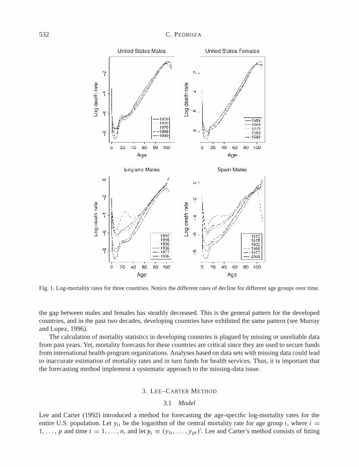
Mortality rates for developed countries declined dramatically during the past century. Improvements instandards of living, sanitary conditions, hygiene, and medicine led to rapidly decreasing infant mortalityrates in the early part of the century and consequently to first increasing and then decreasing mortalityin older age groups in the latter part of the 20th century. Figure 1 shows log-mortality rates for the U.S.obtained from the Human Mortality Database (2002). By mortality rates, we mean the ratio of deaths tomid-year population size for a given interval of age and time (central mortality rates). Figure 1 showsthe constant decline of mortality rates over the last four decades for all-cause mortality in the U.S. formales and females. This is the general pattern for developed countries as illustrated by the two graphs ofEngland and Spain male mortality shown in the bottom panels of Figure 1. This figure also illustrates the‘arm-shaped’ profile of log-mortality across age groups.

In the youngest ages, high mortality rates are attributable to perinatal conditions. Mortality decreasesduring childhood and then increases again to the ‘accident hump’ (traffic accidents and teenage violence)at the ages of 15–20. The rates then steadily increase across older age groups. Over the past five decades,mortality rates have declined for all age groups but at different rates. Age groups 0–10 have declined atthe fastest rates, while the oldest ages have declined at a much slower pace. This holds true for both malesand females in developed regions (Murray and Lopez, 1996).

Overall, females experience lower mortality rates than males. The decade of 1965–1975 marks theperiod with the widest gap between males and females at the oldest ages. However, in the past decade,

532 C. PEDROZA

Fig. 1. Log-mortality rates for three countries. Notice the different rates of decline for different age groups over time.

the gap between males and females has steadily decreased. This is the general pattern for the developedcountries, and in the past two decades, developing countries have exhibited the same pattern (see Murrayand Lopez, 1996).

The calculation of mortality statistics in developing countries is plagued by missing or unreliable datafrom past years. Yet, mortality forecasts for these countries are critical since they are used to secure fundsfrom international health-program organizations. Analyses based on data sets with missing data could leadto inaccurate estimation of mortality rates and in turn funds for health services. Thus, it is important thatthe forecasting method implement a systematic approach to the missing-data issue.

3. LEE–CARTER METHOD

3.1 Model

Lee and Carter (1992) introduced a method for forecasting the age-specific log-mortality rates for theentire U.S. population. Let yit be the logarithm of the central mortality rate for age group i , where i =1, . . . , p and time t = 1, . . . , n, and let yt ≡ (y1t , . . . , ypt )

′. Lee and Carter’s method consists of fitting

A Bayesian forecasting model 533

the following model to the log-mortality rates yt :

yt = ααα + βββκt + εεεt . (3.1)

Here, ααα and βββ are vectors of unknown parameters, εεεt is a vector of error terms, and κt is an unobservedtime series process. The parameters ααα, βββ, and κ are to be estimated. The vector ααα measures the generalpattern of mortality for each age group, and βββ measures the relative rate of change of mortality at eachage. The vector kt is an index of the level of mortality. To ensure identifiability, Lee and Carter imposethe following constraints: ∑

i

βi = 1,∑

t

κt = 0. (3.2)

3.2 Estimation of parameters

Lee and Carter propose the use of singular value decomposition (SVD) to estimate the parameters in themodel. Let Y be a p × n matrix of the log-mortality rates. The vector ααα is estimated by the average log-mortality over time for each age group. SVD is then applied to the mean corrected log-mortality ratesY − ααα:

Y − ααα = UDV ′,where D is a diagonal matrix containing singular values and both U and V are orthogonal matrices. βββ isset equal to the first column of U, and the κt values are set equal to the product of the first column of Vand the leading singular value d1 along with the normalizations given in (3.2). This estimation amounts tousing the first principal component of the log-mortality matrix, as first presented by Bozik and Bell (1987)and Bell and Monsell (1991).

3.3 Modeling and forecasting κt

After κt is estimated by SVD, one can make various adjustments to the estimated vector to produce acloser correspondence between estimated and observed death rates (see Lee, 2000, for further details). Anappropriate univariate autoregressive integrated moving average (ARIMA) time series model forecasts theκt series. Lee and Carter proposed a random walk model with drift for κt , and most applications utilizethe same approach. This model can be expressed as

κt = κt−1 + θ + ωt , (3.3)

where θ is the drift parameter which models a linear trend and ωt is an error term. The mean forecastvalue of κt is calculated as

κn+l = κn + l θ ,

for the lth step-ahead forecast. Finally, to obtain mean forecasts of the log-mortality rates, the meanforecasted values of κt are implemented along with the estimated values of ααα and βββ. The mean forecastof the log-mortality rate for year n + l is

yn+l = ααα + βββκn+l .

3.4 Prediction intervals

To calculate prediction intervals, Lee and Carter’s method first expresses the squared standard error of theforecasted mortality index κn+l for the lth year-ahead forecast from model (3.3) as

σ 2κn+l

= l2σ 2θ + lσ 2

ω,

534 C. PEDROZA

where σ 2θ is the squared standard error of θ and σ 2

ω is the estimate of the variance of the error term ω. TheLee–Carter 95% prediction intervals for the log-mortality rates are computed as

yn+l ± 1.96βββσκn+l .

As pointed out by Lee and Carter (1992, p. 669), this prediction interval ignores errors in estimatingthe parameters ααα, βββ, and the variance of the error term εεε. It only accounts for the error of forecasting κt .Their assumption is that the forecast error dominates all other errors. However, they do point out that forshort-term forecasts their prediction intervals underestimate the ‘true’ forecast error.

The Lee–Carter method has several advantages. First, it is a parsimonious model which accountsfor a large proportion of the variance in the log-mortality rates. Second, the Lee–Carter method uses timeseries methods to generate stochastic forecasts, and it provides probabilistic prediction intervals. The maincriticism of the method is the assumption of a time-invariant age component, i.e. no age–time interaction.From historical data, it appears that this assumption is invalid. For example, the rate of decline in U.S.mortality during the 1990s is different than the one exhibited in the 1970s. Furthermore, infant mortalityexperienced the largest decrease in the early part of the century, whereas older age groups exhibitedthe largest decline in the latter part of the 20th century. Data from other developed countries also showdifferent patterns for different age groups (Booth et al., 2002). These violations raise important questionsabout the applicability of the Lee–Carter method for forecasting mortality in these countries.

4. BAYESIAN MODEL

Lee and Carter’s method for forecasting mortality rates consists of (1) first fitting model (3.1) and (2)then forecasting the series κt using an appropriate time series model. As first presented in Pedroza (2002,p. 48), the Lee–Carter method can be reformulated as a state-space model:

yt = ααα + βββκt + εεεt , εεεtiid∼ Np(0, σ 2

ε I ), (4.1)

κt = κt−1 + θ + ωt , ωtiid∼ N(0, σ 2

ω), (4.2)

where εεεt and ωt are assumed to be independent, and a random walk with drift model is assumed for thestate vector. The multivariate normal model for the log-mortality rates provides a joint distribution for thep age groups at any given point in time. It assumes that the observations are independent across time,that is, the yt are independent identically distributed (iid) with common variance σ 2

ε . In order to compareresults from this model to those obtained from Lee and Carter’s original model, the same constraints thatLee and Carter invoke, i.e.

∑i βi = 1 and

∑t κt = 0, are used. Alternatively, any proper prior distribution

on these parameters will lead to a valid posterior distribution. State-space models are extensively used intime series analysis (see, for example, Harvey, 1990; West and Harrison, 1997). Expressing the Lee–Carter method as a state-space model formalizes it as a statistical model. It also permits simultaneousestimation of all parameters, providing a systematic error assessment.

The Kalman filter can be used to estimate and forecast state-space models (Mehra, 1979; Harvey,1990; Durbin and Koopman, 2001). Forecasting and handling of missing data in state-space models isstraightforward with the Kalman filter. However, this algorithm does not incorporate uncertainty fromunknown parameters and missing observations into either the forecasts or forecasting error. The forecastapproach taken here follows the Bayesian forecasting methods of West and Harrison (1997) and makesuse of simulation methods. The Kalman filter is incorporated into the fitting algorithm. Markov chainMonte Carlo (MCMC) methods are used to draw samples from the joint posterior distribution of theparameters and to form the posterior predictive distribution of the log-mortality rates. In particular, the

A Bayesian forecasting model 535

Gibbs sampler is used to fit the model and to forecast the rates. One advantage of the Bayesian approachis that uncertainty of the parameters ααα, βββ, and θ is incorporated in the estimation and forecasting of κκκ .

Under a Bayesian paradigm, an investigator is able to formally incorporate prior information or knowl-edge about the problem at hand. This prior information is then combined with the observed data to formthe posterior distribution of the parameters on which inference is based. Here, noninformative priors areused which lead to results comparable to those derived from Lee–Carter’s original method. Standard flatprior distributions are assumed for ααα, βββ, and θ along with noninformative priors for the variance param-eters σ 2

ε and σ 2ω: p(ααα, βββ, θ) ∝ 1, p(σ 2

ε ) ∝ 1/σ 2ε , p(σ 2

ω) ∝ 1/σω. The initial prior distribution for thestarting point κ0 is specified as N(a0, Q0), where a0 and Q0 are assumed to be known.

4.1 Implementation

To implement the Bayesian model, the joint posterior distribution of all unknown parameters ααα, βββ, κκκ , θ ,σ 2

ε , and σ 2ω needs to be obtained. However, obtaining posterior inferences analytically from such a high-

dimensional distribution is complicated. Instead, MCMC methods are employed to obtain the posteriordistribution of the parameters. More specifically, we use a Gibbs sampler (Geman and Geman, 1984;Gelfand and Smith, 1990) to draw samples from the joint posterior distribution. This algorithm consists ofiteratively sampling from the conditional distribution of each of the parameters given assigned values toall the other parameters and the data. For the state-space model, the Gibbs sampler consists of two mainsteps: (1) drawing parameters ααα, βββ, θ , σ 2

ε , σ 2ω from their respective conditional distributions given fixed

values for all other parameters and observed data and (2) simulating the state vector κκκ .One way to sample from the state vector is by using the single-state Gibbs sampler which consists

of sampling from p(κt |y, κκκ t , φ), where κκκ t is κκκ excluding κt and φ indexes all other parameters. How-ever, this algorithm can be extremely inefficient. Fruhwirth-Schnatter (1994) and Carter and Kohn (1994)independently developed methods for simulating the state vector based on the identity:

p(κ1, . . . , κT |y) = p(κT |y)p(κT −1 |y, κT ) · · · p(κ1|y, κ2, . . . , κT ). (4.3)

De Jong and Shephard (1995) developed a similar method which samples the disturbance vectors in-stead of the state vectors. This method could also be used for the Lee–Carter model. Here we follow theapproach of West and Harrison (1997) and use the identity given in (4.3) to sample the vector κκκ .

Next we give the steps of the Gibbs sampler. Let Y n be the observed data up to time n.

1. Run the Kalman filter with updating equations

νννt = yt − ααα − βββat , Qt = βββ Rtβββ′ + σ 2

ε I, Kt = Rtβββ′Q−1

t ,

at+1 = at + θ + Ktνννt , Rt+1 = Rt (1 − Ktβββ) + σ 2ω,

for t = 1, . . . , n, and store quantities at , Qt , and Rt . Next, sample the state vector as follows(dependance on all other parameters is implicit):

(a) Sample κn from (κn|Y n) ∼ N(an, Qn), then

(b) for each t = n − 1, n − 2, . . . , 1, 0, sample κt from p(κt |κt+1, Y n).

The conditional distribution for item (b) is

(κt |κt+1, Y n) ∼ N(ht , Ht ),

where

ht = at + Bt (κt+1 − at+1), Ht = Qt − Bt Rt+1 B ′t , and Bt = Qt R−1

t+1.

536 C. PEDROZA

2. Draw σ 2ε from

σ 2ε |Y n, κκκ, ααα, βββ ∼ Inv-Gamma

(pn

2,

∑i∑

t (yit − αi − βiκt )2

2

).

3. Draw ααα and βββ by performing separate regressions for each age group of yi on κκκ . Letting X = (1, κκκ),where 1 is an n × 1 vector of ones and κκκ is the vector of κt values, the conditional distribution of αi

and βi for age group i is

(αi , βi )|Y n, κκκ, σ 2ε ∼ N((X ′ X)−1 X ′y, σ 2

ε (X ′ X)−1).

4. Draw θ from

θ |κκκ, κ0 , σ2ω ∼ N

(κn − κ0

n,σ 2

ω

n

).

5. Draw σ 2ω from

σ 2ω|κκκ, κ0 , θ ∼ Inv-Gamma

(n − 1

2,

∑nt=1(κt − κt−1 − θ)2

2

).

Repeat steps 1 through 5 until convergence.

4.2 Prediction

In general, the posterior predictive distribution ( yn+1|Y n) for future observations can be expressed as

p( yn+1|Y n) =∫

p( yn+1|φ, Y n)p(φ|Y n)dφ =∫

p( yn+1|φ)p(φ|Y n)dφ,

where φ indicates all parameters in the model. The last equation holds because of the assumption thatyn+1 and Y n are conditionally independent given the parameters φ. The posterior predictive distributioncan be obtained analytically or through simulation methods. Here, it is obtained by sampling iterativelyfrom p(φ|Y n) and p( yn+1|φ) to form the distribution.

Given the draws from the posterior distribution obtained from the Gibbs sampler, it is straightforwardto forecast the log-mortality rates, yt . First, samples from the predictive distribution of κt are obtainedfrom (4.2) and then samples from the predictive distribution of yt are generated from (4.1).

These steps can be incorporated into the Gibbs sampler once convergence is attained as follows. Sup-pose we have l = 1, . . . , L draws of all the parameters from the Gibbs sampler and let ϕ(l) indicate thelth draw from the Gibbs sampler of the parameter ϕ. To forecast, we perform the following two steps:

1. Draw κ(l)n+1 from

κ(l)n+1 ∼ N

(κ(l)

n + θ(l), σ 2ω

(l))

.

2. Draw y(l)n+1 from

y(l)n+1 ∼ N

(ααα(l) + βββ(l)κ

(l)n+1, σ

2ε

(l)I)

.

Repeat steps 1 and 2 for j = 1, . . . , N , where N is the number of step-ahead forecasts desired. Theresulting samples of y form the predictive distribution of the mortality rates on which inferences arebased.

A Bayesian forecasting model 537

4.3 Missing data

Mortality data can have missing observations across time and/or age groups. However, it is much morecommon to have incomplete time series data. Li et al. (2004) present a method for applying the originalLee–Carter model to forecast mortality for data sets with few observations over time and complete dataacross age groups. Their method accounts for extra variability arising from fewer time points when fore-casting the κκκ parameter. However, their method does not account for the extra variability which will alsobe present in the ααα and βββ parameters, and it is not meant to handle incomplete data across age groups.

To account for missing observations across time and/or age groups, we can use Rubin’s (1987) methodof multiple imputation. Briefly, multiple imputation replaces each missing value with m different valuesto create m complete data sets. Each complete data set is analyzed as if it was completely observed. Them results are then combined to produce a final inference. This final inference reflects the uncertaintydue to the missing data. To impute the missing values, samples are drawn from the posterior predictivedistribution of the missing values. Letting ymiss and yobs be the vectors of missing and observed data,respectively, and assuming that the missing-data mechanism is ignorable (Little and Rubin, 1987), theposterior predictive distribution is

p(ymiss|yobs) =∫

p( ymiss|yobs, φ)p(φ|yobs)φ.

This is the conditional predictive distribution of ymiss given φ, averaged over the observed-data posteriorof φ. Since the state-space model assumes iid observations over time and across age groups (the covari-ance matrix is assumed to be of the form σ 2

ε I ), the predictive distribution of the missing data given theparameters φ does not depend on the observed data, i.e. p( ymiss|yobs, φ) = p( ymiss|φ). Thus, imputingthe missing values is straightforward regardless of whether the missing data is across time, age groups,or both.

Here, we are mainly interested in computing estimates of the parameters in the model and in form-ing forecasts of the log-mortality rates. To estimate the parameters, we simulate random values of theparameters φ from the observed-data posterior distribution, p(φ|yobs). This can be carried out throughsimulation techniques, in particular the Gibbs sampler. The Gibbs sampler in the presence of missing dataconsists of two main steps (Schafer, 1997): (1) imputation of the missing data given both the observeddata and a sample of the parameters and (2) sampling of the parameters given the complete data. The firststep imputes ymiss with a draw from p( ymiss|yobs, κκκ, φ) and the second steps draws the parameters fromp(κκκ, φ|yobs, ymiss). As mentioned above, the conditional distribution of ymiss given the parameters doesnot depend on yobs regardless of whether the missing data is across time and/or age groups. Imputing themissing values consists of drawing from

p( ymiss|κκκ, φ) ∼ N(ααα + βββκκκ, σ 2ε I ).

Thus, in the presence of missing data, the Gibbs sampler has only one extra step. Handling missing dataunder the Bayesian paradigm can be incorporated seamlessly into the algorithm. The resulting forecastsof log-mortality rates account for the uncertainty due to missing data.

5. EXTENSIONS

As noted before, the Lee–Carter method assumes no age–time interaction. As a demonstration of theflexibility afforded by the Bayesian approach, we could let each age group follow its own random walkwith different rates of decline. This level of flexibility is not required. Alternatively, the age groups canbe clustered so that the youngest age groups follow one random walk, the middle age groups follow

538 C. PEDROZA

another, and the oldest age groups follow a third different random walk. By adopting a Bayesian approachto the Lee–Carter method, an array of changes and/or extensions to the original model can be easilyimplemented. In this section, the notation of the model is generalized and some extensions are brieflydiscussed.

The state-space model can be generalized as follows:

yt = ααα + Zµµµt + εεεt , εεεt ∼ N(0, σ 2ε I ),

µµµt = Gµµµt−1 + ψψψ t , ψψψ t ∼ N(0, �).(5.1)

Here, Z and G are the design and state matrices, respectively, which can include unknown parameters.For the state-space model in Section 4, Z = (βββ, 0), µµµt = (κt , θ)′, ψψψ t = (ωt , ηt )

′, � = diag(σ 2ω, 0), and

G =[

1 1

0 1

]. (5.2)

One way to generalize the Lee–Carter model is to change the form of the state equation. Thus, a simplerandom walk with drift model can be replaced by different ARIMA models. For example, an autoregres-sive process of order 1 [AR(1)] process could be used, placing more weight on the latest observationswhen forming forecasts. The only thing that would differ from the original model would be the matrix G:

G =[φ 1

0 1

]. (5.3)

Another way to extend the Lee–Carter model is to allow the drift parameter to vary over time. Fromempirical data, it appears that the rate of decrease of mortality has changed over the last century, sug-gesting that a model with time-dependent drift would be a plausible model. In this case, µµµt = (κt , θt )

′,ψψψ t = (ωt , ηt )

′, G is as in (5.2), and � = diag(σ 2ω, σ 2

η ). Another extension would be to have both anAR(1) process for the κt and a time-dependent drift. The model would then be as above with the matrixG equal to that of (5.3).

The correlation between age groups could also be modeled by changing the first-level covariancematrix to a nondiagonal form. From historical data, older age groups exhibit more variability due to thesmall size of that population. This could be readily incorporated into the model by letting different agegroups or clusters of the groups have different variances. Modeling of the variance–covariance matrixwould complicate the implementation of the model but could potentially allow for a more realistic modelof mortality rates. Barnard et al. (2000) provide a detail discussion on the modeling of covariance matrices.Below, we give details of the Gibbs sampler for a model that assumes different variances for different agegroups but no correlation between the groups. Details of the fitting algorithm for the other extensionsdiscussed are given in the Appendix.

An extension to the Lee–Carter model which assumes different variance for the different age groupscan be expressed in state-space form as

yt = ααα + βββκt + εεεt , εεεtiid∼ N(0, �),

κt = κt−1 + θ + ωt , ωtiid∼ N(0, σ 2

ω),

(5.4)

where � is assumed to be a diagonal matrix with up to p different σ 2j variance parameters along the

diagonal. Thus, if we grouped the age groups into three clusters of young, middle, and old, then we wouldhave three σ 2

j parameters. Assuming that the variance parameters σ 2j are independent a priori, steps 1–3

A Bayesian forecasting model 539

of the Gibbs sampler change as follows:

1. Run the Kalman filter with updating equations

νννt = yt − ααα − βββat , Qt = βββ Rtβββ′ + �, Kt = Rtβββ

′Q−1t ,

at+1 = at + θ + Ktνννt , Rt+1 = Rt (1 − Ktβββ) + σ 2ω,

Note that the only change occurs in the equation for Qt . Sampling of the state vector κκκ is carriedout as described in Section 4.1.

2. For each cluster of age groups j , draw σ 2j from

σ 2j |Y n, κκκ, ααα, βββ ∼ Inv-Gamma

(p j n

2,

∑i∈ j

∑t (yit − αi − βiκt )

2

2

).

where p j is the number of age groups in cluster j .3. Draw ααα and βββ by performing separate regressions for each age group of yi on κκκ . Letting X = (1, κκκ),

where 1 is an n × 1 vector of ones and κκκ is the vector of κt values, the conditional distribution of αi

and βi for age group i belonging to cluster j is

(αi , βi )|Y n, κκκ, σ 2j ∼ N((X ′ X)−1 X ′y, σ 2

j (X ′ X)−1).

Steps 4 and 5 of the Gibbs sampler are unchanged.The prediction of future values of yt is replaced by drawing from the following normal distribution

yn+1 ∼ N(ααα + βββκn+1, �).

If missing data are present across time, the only change in the imputation of missing observations ison the distribution used. Namely, the covariance matrix changes and the missing values are drawn fromthe multivariate normal distribution

p( ymiss|κκκ, φ) ∼ N(ααα + βββκκκ,�).

If missing data are present across age groups, the imputations will consist of sampling from a conditionalnormal distribution. The methods for multivariate data presented in Schafer (1997) can be used to carryout the imputations.

6. APPLICATION

We analyze a data set for U.S. male all-cause mortality to demonstrate the Bayesian model for forecastingmortality. The data set was obtained from the Human Mortality Database (2002). This data set consists ofannual age-specific death rates for years 1959–1999. The age groups are 0, 1–4, 5–9, . . . , 105–109, 110+.Figure 1, top left panel, shows a plot of the log-death rates for 5 years. To illustrate the methodologypresented here and to assess the predictive quality of the models, we perform out-of-sample forecast forthe last 10 years of the data. That is, we use the data from 1959 to 1989 to fit the model and then forecastfor 10 years ahead. We then compare the forecasts to the observed values.

We fitted and forecasted log-mortality rates using both the original Lee–Carter method and theBayesian model presented in Section 4. For the Bayesian model, we used normal distribution with amean of 5 and variance of 10 as a prior distribution for the starting point of the state process, κ0, based onresults from previous studies. We consider a variance of 10 to be large enough to consider this a ‘vague’

540 C. PEDROZA

prior so as to lead to comparable results to those derived from Lee–Carter’s original method. However,different choices of the prior distribution, in particular different values for the variance, lead to virtuallyidentical results. Here, we summarize the results by presenting the out-of-sample forecasts and predictionintervals from both models.

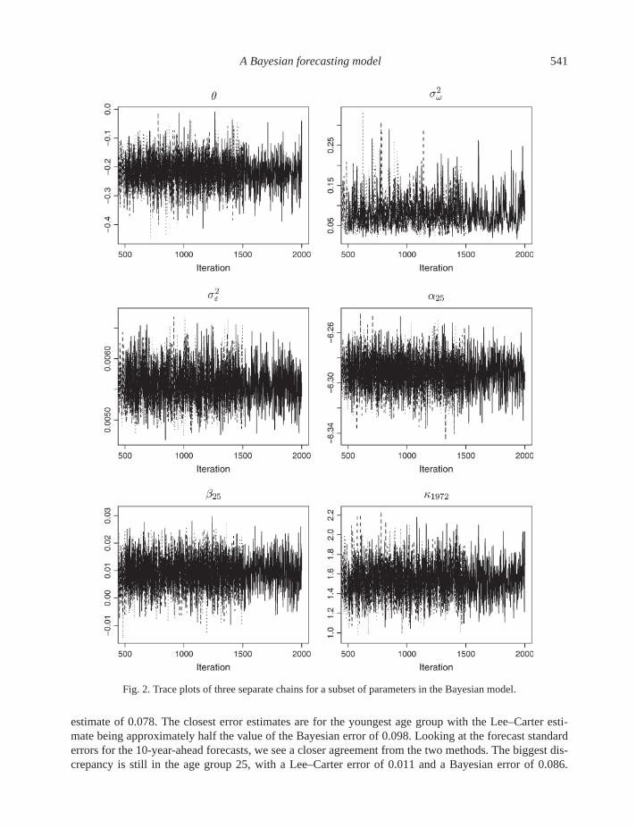
For the Bayesian model, we ran three parallel chains of the Gibbs sampler with different overdispersedstarting values for 2000 iterations. Convergence of the chains was checked using the Gelman–Rubinconvergence diagnostic statistic (Gelman and Rubin, 1992) implemented in the CODA package for R(Plummer et al., 2005). This statistic is computed for each scalar estimate of interest. A statistic less than1.1 suggests convergence. The Gelman–Rubin statistic was computed for all parameters in the model, andall were less than 1.01, indicating convergence. Trace plots for a representative subset of the parametersare presented in Figure 2. These plots show that the three chains mix well together. A final sample for eachparameter was obtained by selecting the last 1000 values of each of the three chains. Results presentedhere are based on the combined 3000 draws from the posterior distribution.

An appropriate concern would be computational cost. Each of the analyses (implementation ofthe model and prediction of the log-mortality rates) presented here took 5 min or less to run in R (RDevelopment Core Team, 2005) on a personal computer with 3.2 GHz and 1 GB of memory. However,computational efficiency was not optimized.

Estimates of the parameters ααα and βββ obtained from the Lee–Carter method and the Bayesian modelare shown in Table 1. These sets of estimates are almost identical for all age groups.

6.1 Display of the forecasts

For each of the p = 24 age groups, we present a graph of the observed log-mortality rates (solid line) foryears 1990–1999 along with the point estimate of the forecast (dashed line) and 95% prediction intervals(dotted lines) (Figure 3). For the Bayesian model, the point estimate is the mean of the posterior predictivedistribution. Figure 3 displays the results for a subset of five representative age groups from both the Lee–Carter method (left panel) and the Bayesian model (middle panel). The two features to focus on in thesegraphs are the accuracy of the point estimates and the coverage of the observed values by the predictionintervals. Comparing first the point forecasts, it appears that forecasts from the Bayesian and Lee–Cartermethod are very close. We calculated the mean squared error (MSE) and averaged it over the age groups:

MSE =∑

i

∑t

( yit − yi t )2/pn,

where yi t indicates either the Bayesian or Lee–Carter forecast for age group i and year t . The averageMSE was 0.0098 for the Bayesian forecasts and 0.0104 for the Lee–Carter ones, indicating a very closeagreement between the two sets of forecasts. There does not appear to be a clear pattern of over- orunderestimation from these two methods.

Comparison of the prediction intervals yields very different results from the two methods. The Lee–Carter intervals for age groups 15–40 are quite narrow. The reason being that for these age groups the βββparameters are very close to zero (Table 1), indicating that the relative rate of decline of mortality is closeto zero. In other words, mortality for these age groups has seen a very small decline relative to other agegroups. Given its role in the prediction interval, the magnitude of the βββ parameter makes the intervals onthese age groups quite small. Overall, the prediction intervals obtained from the Bayesian model are widerthan the Lee–Carter intervals. This is not a surprising result given the fact that this model incorporates allsources of variation in the model when creating forecasts and intervals. The majority of the Bayesianintervals cover the observed rates except for the oldest age groups which exhibit the most variability.

The 1-year-ahead forecast standard errors yield the starkest difference between the Bayesian and Lee–Carter model. For age group 25, the Lee–Carter error of 0.003 is 25 times smaller than the Bayesian

A Bayesian forecasting model 541

Fig. 2. Trace plots of three separate chains for a subset of parameters in the Bayesian model.

estimate of 0.078. The closest error estimates are for the youngest age group with the Lee–Carter esti-mate being approximately half the value of the Bayesian error of 0.098. Looking at the forecast standarderrors for the 10-year-ahead forecasts, we see a closer agreement from the two methods. The biggest dis-crepancy is still in the age group 25, with a Lee–Carter error of 0.011 and a Bayesian error of 0.086.

542 C. PEDROZA

Table 1. Parameter estimates for the Lee–Carter (LC) and Bayesian models

Age group ααα βββ

LC Bayesian Extended LC Bayesian Extended

0 −3.9834 −3.9834 −3.9834 0.1543 0.1548 0.15201–4 −7.1189 −7.1190 −7.1190 0.1063 0.1063 0.10425–9 −7.7961 −7.7964 −7.7961 0.1079 0.1079 0.1065

10–14 −7.7148 −7.7151 −7.7148 0.0796 0.0794 0.078315–19 −6.5999 −6.5997 −6.6000 0.0296 0.0285 0.029520–24 −6.2755 −6.2756 −6.2761 0.0248 0.0238 0.024925–29 −6.2920 −6.2917 −6.2919 0.0101 0.0093 0.010030–34 −6.1792 −6.1793 −6.1791 0.0137 0.0131 0.013435–39 −5.8984 −5.8983 −5.8985 0.0412 0.0406 0.040840–44 −5.4982 −5.4983 −5.4981 0.0665 0.0661 0.065945–49 −5.0396 −5.0396 −5.0397 0.0729 0.0726 0.072450–54 −4.5676 −4.5678 −4.5677 0.0714 0.0715 0.071255–59 −4.1285 −4.1284 −4.1287 0.0641 0.0640 0.063860–64 −3.7038 −3.7037 −3.7037 0.0592 0.0592 0.059165–69 −3.3011 −3.3012 −3.3010 0.0577 0.0576 0.057570–74 −2.9102 −2.9102 −2.9103 0.0469 0.0468 0.046975–79 −2.5287 −2.5286 −2.5283 0.0426 0.0426 0.042680–84 −2.1288 −2.1288 −2.1282 0.0344 0.0343 0.034285–89 −1.7311 −1.7310 −1.7305 0.0326 0.0326 0.032390–94 −1.3700 −1.3703 −1.3702 0.0258 0.0258 0.025895–99 −1.0612 −1.0612 −1.0613 0.0117 0.0117 0.0115

100–104 −0.9447 −0.9446 −0.9447 −0.0238 −0.0243 −0.0242105–109 −1.0464 −1.0462 −1.0464 −0.0618 −0.0616 −0.0597

110+ −1.2933 −1.2932 −1.2935 −0.0679 −0.0622 −0.0589

The Lee–Carter method gives an error of 0.175 for age group 0 compared to the Bayesian error of 0.181for this group. Thus, for long-term forecasts, it appears that the Lee–Carter forecasting error starts to ap-proach the Bayesian error, but for most age groups, it is still less than 75% of the error obtained from theBayesian model.

The assumption made by Lee and Carter that the main source of error would come from the forecastingerror of the mortality index κt yields prediction intervals which are too narrow for short-term forecasts,specially for young adults and older age groups. When we account for all sources of estimation error,we calculate prediction intervals which are wider and reflect the true prediction error in the forecastedmortality rates.

6.2 Model diagnostics

From the plots of the forecasted log-mortality rates, it appears that for some of the age groups (e.g.50 and 90), the prediction intervals are too wide. One assumption of the fitted model is that all agegroups have the same variability. However, plots of the observed data from 1959 to 1989 show that someage groups have more variability than others. In particular, the oldest age group appears to be morevariable than all the other groups as would be expected. To test the assumption of homogeneity acrossage groups, we can look at posterior predictive diagnostics (Gelman et al., 1996). This approach consistsof replicating data from the model and then comparing it to the observed data. Any systematic differences

A Bayesian forecasting model 543

Fig. 3. Observed (solid line) and forecasted (dashed line) log-mortality rates with 95% prediction intervals for U.S.males for Lee–Carter’s method (left panel), Bayesian model (middle), and extended Bayesian model (right).

between the replicated and observed data could indicate a misfit in the model. Differences or discrepanciesbetween the model and data can be measured by a test quantity or discrepancy measure. This measure candepend on either just data (i.e. test statistic) or both data and parameters. The posterior predictive checkis the comparison between realized values of the measure D(y, φ∗) obtained from the observed data yand simulated parameters φ and the predictive measures D(y∗, φ∗) obtained from simulated data and

544 C. PEDROZA

parameters. If the actual data are plausible, then the posterior distribution of D(y, φ∗) will be similar tothat of D(y∗, φ∗).

As a discrepancy measure here, we calculate the average squared residual for each age group as

e2i = 1/n

∑t

(yit − αi − βiκt )2.

Let e2i ( y∗; φ∗) be the value of the discrepancy measure for the simulated data y∗ and simulated param-

eters φ∗ for age group i and e2i ( y; φ∗) the value of the measure for the actual data and simulated pa-

rameters. This provides an estimate of the regression variance. The approximate posterior distributions of(e2

i ( y; φ∗), e2i ( y∗; φ∗)) based on the same 500 draws of the parameters and simulated data are shown in

Figure 4 (left panel) for a subset of the age groups.If the posterior distributions of the discrepancy for the simulated data and the actual data are similar,

then we should see large portions of the distribution of the discrepancies lie both above and below thediagonal line (e2

i ( y; φ∗) = e2i ( y∗; φ∗)). For age groups 0 and 25, this seems to be the case, indicating

that the observed variability is similar to the expected variability under the Bayesian model. However, forage groups 50 and 90, almost all the points lie above the diagonal, indicating that the variability under themodel is much larger than the observed one for these two age groups. In other words, we overestimate thevariability for these age groups. In contrast, the plot for the oldest age group 110 shows a clump of pointsall well below the diagonal, indicating that the observed variability is much larger than that expected underthe model. These results indicate a lack of fit of the model to the observed data. From these graphs, wecan conclude that there is evidence of heterogeneous variances for different age groups.

The posterior predictive diagnostics seem to indicate that a model with different variances for differentage groups may be more appropriate. To keep the model as simple as possible, age groups may be groupedinto clusters which exhibit similar variances. To help construct these clusters, we examined the approxi-mate posterior distributions of the average squared residuals (i.e. approximate estimates of the regressionvariances) obtained from the actual data. The means of these distributions for the age group 24 are shownin Table 2. To try to capture the largest differences between the age groups, we decided on a model with10 different variance parameters. We clustered the age groups as follows: 0, 1, 5–10,15–35, 40, 45–65,70–80, 85–100, 105, 110. We fitted this model and again calculated the discrepancy measures for bothactual and simulated data. This analysis took between 5 and 7 min to run in R. The resulting posterior dis-tributions are shown in Figure 4 (right panel). Here we see that the values for the discrepancies are muchmore evenly distributed above and below the diagonal line, indicating a better fit to the observed data.

Plots of the forecasts from the extended model are shown in Figure 3 (right panel). Here we seethe same pattern as for the simulated in-sample data. Prediction intervals for the younger age groupsdo not differ much from the ones produced by the original model. For the middle groups (i.e. 50–90)the intervals are narrower, and for the oldest group, the interval is much wider and covers the observedvalues. In general, the prediction intervals are much tighter for age groups which have historically shownsmaller variability. The prediction intervals are improved, although the point estimates of the forecast donot change by much.

7. CONCLUSIONS

This paper has presented a Bayesian approach to the Lee–Carter method for forecasting mortality rates.The Bayesian formulation of the model incorporates all sources of variation in the model when formingforecasts. The resulting prediction intervals are much wider than those obtained by Lee–Carter, and theyreflect more accurately the forecasting error associated with the model. Furthermore, the Bayesian modelcan easily handle missing data both in the time series and across age groups and incorporate the uncertainty

A Bayesian forecasting model 545

Fig. 4. Scatter plot of the joint posterior distribution of the averaged squared residual e2i for age group i evaluated with

observed data and simulated parameters vs. simulated data and parameters. Left panel corresponds to data simulatedfrom the model assuming homogeneity of variance across age groups and the right corresponds to data simulatedassuming heterogeneity.

associated with it. This aspect of the model is important when working with data from countries wherevital records are incomplete or unreliable.

We compared results from the Bayesian model and the Lee–Carter model for U.S. male data andshowed that confidence interval widths are different. For some age groups, the Lee–Carter intervals do

546 C. PEDROZA

Table 2. Approximate estimates of the regression variance for homogenous Bayesian model

Age group Estimated variance

0 0.00541–4 0.00305–9 0.0012

10–14 0.001415–19 0.009520–24 0.008025–29 0.004530–34 0.004335–39 0.004740–44 0.001845–49 0.001050–54 0.000855–59 0.001060–64 0.000865–69 0.000770–74 0.000875–79 0.000880–84 0.000785–89 0.001090–94 0.001395–99 0.0013

100–104 0.0021105–109 0.0089

110+ 0.0690

not cover the observed values. In contrast, the Bayesian intervals cover the observed values and reflect thetrue uncertainty of these forecasts. As an extension, we also fitted a model with heterogeneous variance forthe age groups. This extension models the observed variability for different age groups and provides morerealistic confidence intervals for the estimated log-mortality rates as well as prediction intervals for futureobservations. Another possible extension to the model would be to allow age groups to have different ratesof decline. We could also let each age group have its own time-dependent drift. This model would alloweach age group to have different rates of decline and also allow these rates to vary over time. Also notethat different prior specifications for the model parameters can be used to incorporate prior information.

We realize that implementation of the Bayesian model is more complex. However, we believe that itis important for forecasts and their estimated errors to reflect the underlying uncertainty of the model anddata. Furthermore, a Bayesian analysis allows the investigator to test the validity of the model through theuse of posterior predictive checks as demonstrated in Section 6.2. We refer the reader to Gelman et al.(1995, 1996) for a more in-depth discussion of model checking in a Bayesian setting.

A second disadvantage of the Bayesian approach is in the specification of prior information. If trueprior information is known, it should be incorporated into the Bayesian model. However, it is not alwayseasy to quantify prior information in terms of a prior distribution. Careful consideration needs to be givento the prior specifications, and sensitivity analysis should be conducted to check how robust the forecastsare to the choice of the prior distribution.

One aspect of the Bayesian approach taken here is worthy of discussion. We implicitly used a squared-error loss when determining the Bayesian estimator for the forecasts. This loss function penalizes equallyunderestimation and overestimation. However, suppose we want forecasts for a developing country to

A Bayesian forecasting model 547

decide funding for a public health program. In this case, underestimation would be a far worse loss thanoverestimation. Here, a linear loss would be more appropriate. The Bayes estimate of the mortality fore-casts would then be an appropriate percentile of the posterior predictive distribution. For example, ifwe deemed underestimation to be three times worse than overestimation, then we would use the 75thpercentile as the estimate. For a different country, the estimate could possibly be another percentile, de-pending on the intended use of the forecasts. Tailoring a model to a specific data set is one of the mostimportant advantages of a Bayesian analysis. A better fitting prediction model can lead to more realisticforecasts and prediction intervals of mortality rates.

ACKNOWLEDGMENTS

The author thanks Lemuel Moye, Robert Hardy, and David van Dyk for their insightful and constructivecomments. Helpful comments by the associate editor and two referees have greatly improved the article.Conflict of Interest: None declared.

APPENDIX

A.1 The Gibbs sampler for extended models

The general model presented in (5.1) can be fitted by the Gibbs sampler. Assuming noninformative priorsfor the parameters, the steps of the Gibbs sampler are as follows:

Gibbs sampler for general model.

1. Run the Kalman filter with the following updating equations

νννt = yt − ααα − Zat , Qt = Z Rt Z ′ + σ 2ε I,

Kt = G Rt Z ′Q−1t , Lt = G − Kt Z ,

at+1 = Gat + Ktνννt , Rt+1 = G Rt L ′t + �.

Store quantities at , Qt , and Rt for t = 1, . . . , n. Next, sample the state vector as follows:

(a) Sample µµµn from (µµµn|Y n) ∼ N(an, Qn), then

(b) for each t = n − 1, n − 2, . . . , 1, 0, sample µµµt from p(µµµt |µµµt+1, Y n).

The conditional distribution for item (b) is

(µµµt |µµµt+1, Y n) ∼ N(ht , Ht ),

where

ht = at + Bt (µµµt+1 − at+1), Ht = Qt − Bt Rt+1 B ′t , and Bt = Qt G

′ R−1t+1.

2. Draw σ 2ε from Inv-Gamma(pn/2,

∑t (yt − ααα − Zµµµt )

′(yt − ααα − Zµµµt )/2).3. Draw ααα and Z by performing separate regressions of yi on µµµt for each age group. Letting X =

(1, µµµ), the conditional distribution of αi and Zi for age group i is

(αi , Zi )|Y n, µµµ, σ 2ε ∼ N((X ′ X)−1 X ′y, σ 2

ε (X ′ X)−1).

548 C. PEDROZA

4. Draw � from its conditional distribution. Assuming the prior

p(�) ∝ |�|−(d+1)/2,

where d is the dimension of �, then the conditional distribution is an inverted-Wishart distribution:

p(�|µµµ) ∼ IWd(n, S−1),

where S = ∑t (µµµt − Gµµµt−1)(µµµt − Gµµµt−1)

′.

Gibbs sampler for AR(1) model. In the case with an AR(1) process in the state equation, the modelbecomes

yt = ααα + βββκt + εεεt , εεεtiid∼ N(0, σ 2

ε I ),

κt = φκt−1 + θ + ωt , ωtiid∼ N(0, σ 2

ω).

The Gibbs sampler has an added step for drawing the parameter φ. The steps for this model are as follows:

1. Run the Kalman filter using the equations for the general model with the matrix G as in (5.2).2. Draw σ 2

ε from Inv-Gamma(pn/2,∑

i∑

t (yit − αi − βiκt )2/2).

3. Draw each αi and βi from N((X ′ X)−1 X ′yi , σ2ε (X ′ X)−1), where X = (1, κκκ).

4. Draw σ 2ω from

σ 2ω|κκκ, κ0 , θ, φ ∼ Inv-Gamma

(n − 1

2,

∑nt=1(κt − φκt−1 − θ)2

2

).

5. Draw φ from

φ|κκκ, θ, σ 2ω, Y n ∼ N

(∑nt=1 κt−1(κt − θ)∑n

t=1 κ2t−1

,σ 2

ω∑nt=1 κ2

t−1

).

REFERENCES

ALHO, J. M. AND SPENCER, B. D. (1990). Error models for official mortality forecasts. Journal of the AmericanStatistical Association 85, 609–616.

BARNARD, J., MCCULLOCH, R. AND MENG, X.-L. (2000). Modeling covariance matrices in terms of standarddeviations and correlations, with application to shrinkage. Statistica Sinica 10, 1281–1311.

BELL, W. AND MONSELL, B. (1991). Using principal components in time series modeling and forecasting of age-specific mortality rates, ASA Proceedings of the Social Statistics Section. Alexandria, VA: American StatisticalAssociation, pp. 154–159.

BOOTH, H., MAINDONALD, J. AND SMITH, L. (2002). Applying Lee-Carter under conditions of variable mortalitydecline. Population Studies 56, 325–336.

BOZIK, J. E. AND BELL, W. R. (1987). Forecasting age specific fertility using principal components, ASA Proceed-ings of the Social Statistics Section. Alexandria, VA: American Statistical Association, pp. 396–401.

BROUHNS, N., DENUIT, M. AND VAN KEILEGOM, I. (2005). Bootstrapping the Poisson log-bilinear model formortality forecasting. Scandinavian Actuarial Journal 212–224.

BROUHNS, N., DENUIT, M. AND VERMUNT, J. K. (2002). Measuring the longevity risk in mortality projections.Bulletin of the Swiss Association of Actuaries, 105–130.

A Bayesian forecasting model 549

CARTER, C. K. AND KOHN, R. (1994). On Gibbs sampling for state space models. Biometrika 81, 541–553.

CARTER, L. (1995). Forecasting U.S. mortality: a comparison of Box-Jenkins ARIMA and structural time seriesmodels. The Sociological Quarterly 37, 127–144.

CARTER, L. R. AND LEE, R. D. (1992). Modeling and forecasting US sex differentials in mortality. InternationalJournal of Forecasting 8, 393–411.

CZADO, C., DELWARDE, A. AND DENUIT, M. (2005). Bayesian Poisson log-bilinear mortality projections. Insur-ance: Mathematics & Economics 36, 260–284.

DE JONG, P. AND SHEPHARD, N. (1995). The simulation smoother for time series models. Biometrika 82,339–350.

DURBIN, J. AND KOOPMAN, S. J. (2001). Time Series Analysis by State Space Methods. Oxford University Press.

FRUHWIRTH-SCHNATTER, S. (1994). Data augmentation and dynamic linear models. Journal of Time Series Analy-sis 15, 183–202.

GELFAND, A. E. AND SMITH, A. F. M. (1990). Sampling-based approaches to calculating marginal densities. Jour-nal of the American Statistical Association 85, 398–409.

GELMAN, A., CARLIN, J. B., STERN, H. S. AND RUBIN, D. B. (1995). Bayesian Data Analysis. London:Chapman & Hall.

GELMAN, A., MENG, X.-L. AND STERN, H. (1996). Posterior predictive assessment of model fitness via realizeddiscrepancies (discussion 760–807). Statistica Sinica 6, 733–760.

GELMAN, A. AND RUBIN, D. B. (1992). Inference from iterative simulations using multiple sequences (with dis-cussion). Statistical Science 7, 457–472.

GEMAN, S. AND GEMAN, D. (1984). Stochastic relaxation, Gibbs distributions, and the Bayesian restoration ofimages. IEEE Transactions on Pattern Analysis and Machine Intelligence 6, 721–741.

GIROSI, F. AND KING, G. (2005). Demographic Forecasting. Monograph (unpublished).

HARVEY, A. C. (1990). Forecasting, Structural Time Series Models, and the Kalman Filter. Cambridge: CambridgeUniversity Press.

HUMAN MORTALITY DATABASE. (2002). University of California, Berkeley (USA), and Max Planck Institutefor Demographic Research (Germany). Available at http://www.mortality.org or http://www.humanmortality.de(accessed on April 1, 2005).

LEE, R. (2000). The Lee-Carter method for forecasting mortality, with various extensions and applications. NorthAmerican Actuarial Journal 4, 80–93.

LEE, R. D. AND CARTER, L. R. (1992). Modeling and forecasting U.S. mortality (discussion 671–675). Journal ofthe American Statistical Association 87, 659–671.

LEE, R. D. AND TULJAPURKAR, S. (1994). Stochastic population forecasts for the United States: beyond high,medium and low. Journal of the American Statistical Association 89, 1175–1189.

LI, N., LEE, R. AND TULJAPURKAR, S. (2004). Using the Lee-Carter method to forecast mortality for populationswith limited data. International Statistical Review 72, 19–36.

LITTLE, R. J. A. AND RUBIN, D. B. (1987). Statistical Analysis with Missing Data. New York: John Wiley & Sons.

MEHRA, R. K. (1979). Kalman filters and their applications to forecasting. In Makridakis, S. and Wheelwright, S. C.(eds), Forecasting. Studies in the Management Sciences, Volume 12. New York: Elsevier, pp. 75–94.

MURRAY, C. J. AND LOPEZ, A. D. (1996). The Global Burden of Disease. Cambridge, MA: Harvard UniversityPress.

PEDROZA, C. (2002). Bayesian hierarchical time series modeling of mortality rates, Ph.D. Thesis, Harvard University,Cambridge, MA.

550 C. PEDROZA

PLUMMER, M., BEST, N., COWLES, K. AND VINES, K. (2005). Coda: Output Analysis and Diagnostics forMCMC. R package version 0.9-2. Available at http://www-fis.iarc.fr/coda/.

R DEVELOPMENT CORE TEAM. (2005). R: A Language and Environment for Statistical Computing. R Foundationfor Statistical Computing, Vienna, Austria. ISBN 3-900051-07-0. Available at http://www.R-project.org.

RUBIN, D. B. (1987). Multiple Imputation for Nonresponse in Surveys. New York: John Wiley & Sons.

SCHAFER, J. L. (1997). Analysis of Incomplete Multivariate Data. London: Chapman & Hall.

WEST, M. AND HARRISON, J. (1997). Bayesian Forecasting and Dynamic Models. New York: Springer.

WILMOTH, J. R. (1995). Are mortality projections always more pessimistic when disaggregated by cause of death?Mathematical Population Studies 5, 293–319.

[Received June 21, 2005; revised January 25, 2006; accepted for publication February 10, 2006]