Forecasting Demand for Fashion Goods:A Hierarchical Bayesian Approach

Phillip M. Yelland

Google Inc., 1600 Amphitheatre Parkway, Mountain View, CA 94043, U.S.A.

phillip.yelland@gmail.com

+1-650-486-4112

Xiaojing Dong

Santa Clara University, 500 El Camino Real, Santa Clara, CA 95053, U.S.A.

xdong1@scu.edu

+1-408-554-5721

Abstract

A central feature of demand for products in the fashion apparel segment is a pronounced product life cycle—demand for a fashion product tends to rise and fall dramatically in accordance with the rate of public ofadoption. Product demands that vary in such a manner can be difficult to forecast, especially in the criticalearly period of a product’s life, when observed demand can be a very unreliable yardstick of demand later on.This paper examines the applicability of a Bayesian forecasting model—based on one developed for use in thecomputer industry—to fashion products. To do so, we use an agent-based simulation to produce a collectionof demand series consistent with commonly-accepted characteristics of fashion adoption. Using Markovchain Monte Carlo techniques to make predictions using the Bayesian model, we are able quantitatively todemonstrate its superior performance in this application.

1. Introduction

According to the US Office of Technology Assessment (1987), the apparel market in the US can bedivided into three segments: 1) fashion products, which have a very short product life cycle, around tenweeks, and account for approximately 35% of the market; 2) seasonal products, which have a slightly longerproduct life cycle of around twenty weeks and account for approximately 45% of the market; and 3) basicproducts, which do not have an obvious sales pattern and are sold throughout the year. The fashion clothingsegment presents a particular challenge for demand planners: Competition is frequently fierce and profitmargins volatile, supply chains span the globe and can be hard to coordinate, and the nature of demandfor fashion goods themselves is (ipso facto) almost invariably highly labile and difficult to predict (Hunterand Valentino 1995). Regarding the latter, the most salient determinant of demand for fashion goods istheir very pronounced product life cycle. Indeed, as Sproles (1981) points out, “[f]ashions are, by definition,temporary cyclical phenomena adopted by consumers for a particular time and situation. . . , having stagesof introduction and adoption by fashion leaders, increasing public acceptance (growth), mass conformity(maturation), and the inevitable decline and obsolescence awaiting all fashions”.

This inherent variability of fashion product demand makes forecasting very difficult, especially early in aproduct’s life cycle, when little is known about the product’s ultimate level of market acceptance; demandearly in a product’s life may give scant indication of demand later on in the life cycle. To quote Kang(1999): “[T]he best-selling item of the last season could be the worst-selling item for the coming season”.Compounding difficulties is the tendency of fashion cycles to shorten in recent years, a phenomenon Kang(ibid.) attributes to advances in media technology and the widespread availability of fashion clothing items.

Preprint submitted to Handbook on Intelligent Fashion Forecasting Systems March 29, 2013

Of course, appreciably short product lifecycles are not confined to the clothing industry; (Yelland 2010)describes a Bayesian forecasting model developed for computer components, where rapid technological de-velopment also leads to very pronounced short lifecycles. We set out to examine the suitability of a similarBayesian forecasting model for demands in the fashion apparel segment, hypothesizing that a model whichhad proven effective in accomodating short product lifecycles held promise for fashion clothing forecasting,too.

In (Yelland 2010), assessment of the forecasting model is based on actual demand experienced by aparticular manufacturer (Sun Microsystems Inc.); the use of actual series was largely a consequence ofthe model’s use by that manufacturer. While the use of manufacturer data in that paper provides theassurance that the model has real-world applicability, in the strictest sense it establishes efficacy only forone particular firm over a particular period of time. To broaden the scope of the model in this work,we adopt a different approach: We simulate plausible demand series for fashion goods options under avariety of circumstances, and test the accuracy of a model derived from (Yelland 2010) in extrapolatingthem. Of course, very little would be achieved if the simulation were constructed along the same lines as theforecasting model itself, merely embodying the parameters and latent constructs used in the model. As Cooket al. (2006) demonstrate, such an exercise can play a valuable role in validating the correctness of a modelimplementation, but it would hardly establish the broad applicability of the model itself. Instead, we usean agent-based simulation to calculate demand based upon individual purchase decisions, with simulationelements designed to drive those individual decisions in a manner consistent with paradigmatic characteristicsof fashion goods and their markets.

In the interests of expositional clarity, we make to simplifications in both the simulation and forecastingmodel used in this chapter, concentrating predominantly on the treatment of the product life cycle. Thusregular cyclical or “seasonal” effects on demand, for example, are represented only in very rudimentaryform; simulation of more complex seasonality represents no challenge, and many models of seasonalityfrom the forecasting literature (such as seasonal dummies) may be added to the forecasting model withoutdifficulty—see Harvey (1989) or Brockwell and Davis (2002) for examples.

The plan of the chapter is as follows: In the next section, we outline related work in the literature. Thefollowing section describes in detail the simulation used to generate option demands. We then introducethe forecasting model, with brief prefatory remarks about the Bayesian approach to forecasting in general.The forecasting performance of the model in respect of the simulated option demands is then appraised incomparison with that of a sophisticated benchmark forecasting method. We finish with concluding remarks.

2. Related Work

As Hines and Bruce (2007) recount, the modern fashion apparel industry is characterized by increasinglyshort product life cycles, which contrast with long lead times and complicated supply chain (typically, ittakes two years from the design and one year from production before a garment is sold). This has ledto a a proliferation of literature studying supply chain management (Donohue 2000), assortment planning(Caro and Gallien 2007), and—most saliently for our purposes—sales forecasting. The latter features studiesusing various probability distributions to fit the sales data and forecast the demand—Agrawal and Smith(1996), for example, fit a negative binomial distribution to retail sales data. In the model recounted here, wesupplement a probability distribution for sales with an explicit account of the product life cycle. This hasmany precedents in forecasting models for technology products—c.f. (Wu et al. 2010), among many others.

We use a Bayesian approach in formulating our model to tackle another challenge often faced by forecast-ers in the fashion apparel industry: A very limited amount of available calibration data. Other researchersin the area have also adopted a Bayesian approach, mostly to account for the dynamic nature of demand up-dates as more data become available. Early inventory models that allow demand updating using a Bayesianapproach include those of Dvoretzky et al. (1952), Scarf (1959), Iglehart (1964), Murray and Silver (1966),Azoury and Miller (1984), Azoury (1985), and Miller (1986). More recently, Iyer and Bergen (1997) modela Quick Response apparel supply contract, allowing the demand distribution to be updated in a Bayesianfashion using early sales data. The demand process in this model is assumed to follow a normal distribution.Other recent studies adopt a two-stage demand process for a fashion product. Gurnani and Tang (1999),

2

for example, allow a retailer to place two orders before the selling season. They derive an optimal orderingpolicy, while allowing the first-stage demand to be updated via a Bayesian method. In a similar setup, Choiet al. (2003) use a newsvendor model in a two-stage context using Bayesian information updating. Otherexamples include (Eppen and Iyer 1997) and (Choi et al. 2006), to name a few.

Besides information updating, the model in this chapter illustrates that the Bayesian approach can alsobe applied using a hierarchical prior, so as to obtain forecasts for a single item with only a small amountof historical sales information by “borrowing” information from similar items. This feature of the Bayesianapproach is widely adopted in the Marketing and Economics literature (see Ansari et al. (2000), Narayananand Manchanda (2009), and Dong et al. (2009), for example). A seminal paper in Marketing is (Rossi et al.1996), where a hierarchical Bayesian framework is adopted to analyze model parameters that are related toindividual customers’ responses to shopping coupons. In this study, each customer makes a limited numberof observed purchases, and individual level inference is not feasible using classical statistics. The hierarchicalBayesian approach, on the other hand, calculates individual level inferences by combining population levelparameter estimates with the individual level data—essentially borrowing information from the rest of thepopulation. Rossi et al. (2005) present a detailed discussion of hierarchical Bayesian methods.

As indicated in section 1, to apply our method in an empirical context, we adopt an agent-based approachto simulate demand data. In general methodological terms, agent-based simulation investigates aggregatelevel phenomena by simulating the behaviors of individual agents (Rand and Rust 2011). This approachallows a proper account to be made of complexity in the data generation process while also being tractable.It has been widely adopted across multiple fields, including organizational science (Cohen et al. 1972),supply chain management (Walsh and Wellman 1999) and Marketing (Goldenberg et al. 2009). North et al.(2010), given an account of Procter & Gamble’s successful of application agent-based simulated to improverevenue. Related to our study, agent-based simulation has also be applied to investigate the diffusion ofinnovation—c.f. for example Schwoon (2006), Delre et al. (2007), Schenk et al. (2007), and Kiesling et al.(2009). Our own agent-based simulation is described in the next section.

3. Data Simulation

1

Our simulation of demand for fashion products over time is based on the parallels—noted by Sproles(1981) among others—between fashion goods lifecycles and the more general process of innovation adproduct.To this end, we adapt Rand and Rust’s (2011) simulation of innovation adproduct. This starts with aset of agents, indexed 1, . . . , N , whose communication patterns take the form of a so-called small-worldnetwork after Watts and Strogatz (1998). The network fixes for each agent i a set of neighbors, Neighborsi,comprising those agents which are in direct communication with agent i. We simulate the actions of this setof agents over periods t = 1, . . . , T .2 In each period t, agent i may elect to purchase the product—an eventwe denote purchit. In the interests of simplicity, we assume that each agent purchases the product once.Furthermore, only a subset of the agents—the product’s “potential market”, Market ⊆ {1, . . . , N}—willever purchase the product. In each period, therefore, agent i’s probability of purchase is non-zero only ifi ∈ Market and i /∈ Purcht−1.3 We abbreviate this conjunction—informally, agent i’s membership of theproduct’s potential market in period t—as potit. When the simulation begins, each agent enters into Market

independently,4 each with the same product-specific probability r. Following a paradigm expressed in modelsof innovation diffusion dating from (at least) Bass (1969), we assume that such purchases are motivatedby either: a) an exogenous influence, which stems from the promotional activities through mass-marketingchannels, such as advertising, or b) an endogenous influence, resulting from communication with neighboring

1A full summary of the notation in the paper, and a description of the probability distributions used is provided in theappendices.

2For concreteness’s sake, we will frequently regard one period as one day, though we use the term “period” throughout toemphasize the generality of the framework.

3For technical convenience, we take Purch0 to be the empty set.4Throughout this section, events are assumed (conditionally) independent unless the contrary is noted.

3

agents who have already purchased the product. The event purch-exit denotes agent i’s exogenously-motivated purchase in period t, and purch-endit similarly denotes an endogenously-motivated purchase.Since a purchase may arise exogenously or endogenously, the event purchit is the conjunction of theseevents, so that purchit = purch-exit ∨ purch-endit.

Provided that agent i is in the product’s potential market in period t, the probability of s/he makingan exogenously-motivated purchase in period t is determined by a parameter pi associated with agent iand a seasonal effect associated with t. As adumbrated in section 1, to keep things simple, the simulationincorporates only one seasonal effect—a “day-of-the-week” effect that distinguishes every 7th period with a50% increase in sales. Thus we have:

p(purch-exit |potit) = min[(1 + 0.5St)pi, 1], (1)

where St is an indicator variable picking out every 7th period:

St =

{1 if t mod 7 = 0,

0 otherwise.(2)

The probability of an endogenously-motivated purchase by agent i in period t (conditional on membershipof the potential market in t) depends on another agent-specific parameter, qi, along with the seasonal effectand the fraction of agent i’s neighbors who have already purchased the product:

p(purch-endit |potit) = min

[(1 + 0.5St)qi

|Neighborsi ∩ Purcht−1||Neighborsi|

, 1

]. (3)

At the outset of the simulation for a particular product, parameters pi and qi for each agent i are sampledfrom the (compound) beta distributions listed below. We use an alternate (and arguably more intuitive)parameterization, Beta(µ, σ2), of the beta distribution in terms of its mean µ and variance σ2, where it isrequired that σ2 < µ(1−µ); the more conventional parameters α and β can be recovered as µν and (1−µ)νresp., for ν = µ(1− µ)/σ2 − 1. In addition, we use the shorthand x ∼ {v1, v2, . . . , vn} to indicate that valueof the random variable x is drawn randomly from the set {v1, v2, . . . , vn}. Then:

pi ∼ Beta(µp, µp/2), where µp ∼ {0.00035, 0.0005, 0.001, 0.005, 0.01, 0.02}, (4)

qi ∼ Beta(µq, µq/2), where µq ∼ {0.05, 0.1, 0.2, 0.4, 0.5}, (5)

Simulating a demand series over periods 1, . . . , T involves the following:

1. Initialize the agent-specific values pi and qi according to the distributions given in (4) and (5) resp.Compute Market according to r, set Purch0 to ∅ and poti1 iff i ∈ Market.

For each time period t:

2. Independently for each agent i such that potit:5

(a) Draw a uniformly-distributed random variable u-exoit ∼ Unif(0, 1). Assert event purch-exit iffu-exoit < p(purch-exit |potit), the latter term being defined in equation (1).

(b) Draw another random variable u-endoit ∼ Unif(0, 1) and assert purch-endit iff u-endoit <p(purch-endit |potit) from equation (3).

(c) Assert purchit iff purch-exit or purch-endit is true.

3. Let Purcht+1 = Purcht ∪ {i ∈ 1, . . . , N | purchit}.

5i.e. i ∈ Market and i /∈ Purcht−1.

4

4. Simulated demand, yt, for the product in period t, is∑Ni=1 I(purchit), where I(purchit) is 1 if purchit

is true, and 0 otherwise.

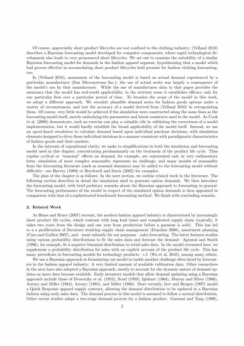
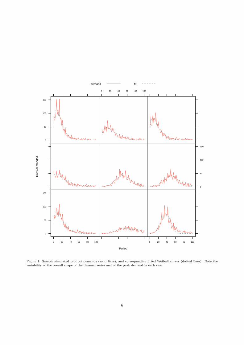
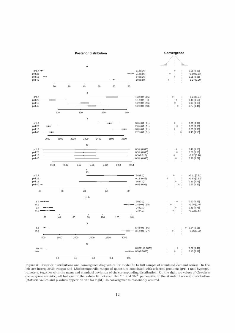
Repeating the simulation procedure a number of times produces a collection of possible trajectories forproduct demand over time. We took a sample of 50 such series, each of 100 periods in length, for use inour forecasting exercises; nine typical sample members appear in figure 1. In next section, we describe theBayesian model proposed for extrapolating these series.

4. Forecasting Model

Before describing the details of forecasting model itself, we outline in general terms how Bayesian methodsare particularly appropriate when forecasting demand for fashion goods.

4.1. Bayesian Forecasting

In the conventional forecasting situation examined in the literature, a suitably long time series of observedvalues—y = (yt, . . . , yT ), say—is presented for extrapolation, and (restricting the discussion to a singleperiod forecast horizon for simplicity) the task of the forecaster is to predict the value of the value of the seriesafter h further periods, yT+h. In the demand forecasting exercise examined here, however, short product lifecycles mean that individual products frequently lack sufficient observed demand values to support reliableextrapolation. In this application, therefore, input to the forecasting process consists not only of previousdemands for a particular product, but also of observed demands for other similar products, too—evenproducts that are no longer available. Thus the data takes the form of a collection of series, y1, . . . ,yJ , ofpotentially differing lengths (some of which may be zero), so that for j = 1, . . . , J , yj = (yj1, . . . , yjTj ). Theaim is to forecast yl Tl+h, for some chosen product l.

The objective of the model presented in this section is a statistical representation of such a collection ofdemand series using a set of unobserved quantities. This latter set—which we denote in the abstract by thevector θ—contains the model parameters, and may also contain the values of latent variables or processes.It is assumed that the representation in terms of θ is sufficiently detailed that all the elements of the seriesare conditionally independent given θ, i.e.:6

p(y1, . . . ,yJ |θ) =

J∏j=1

Tj∏t=1

p(yjt|θ). (6)

A Bayesian forecast of yl Tl+h rests on its posterior predictive distribution. The latter is simply theconditional distribution of yl Tl+h given the historical demands, p(yl Tl+h|y1, . . . ,yJ). The conditional inde-pendence property of the model expressed in equation (6) is pivotal to the derivation of this distribution,since on the assumption that yl Tl+h is also well-represented by θ, it should be conditionally independent ofthe historical demands, just as the historical demands were conditionally independent of each other:

p(yl Tl+h,y1, . . . ,yJ |θ) = p(yl Tl+h|θ)p(y1, . . . ,yJ |θ). (7)

Now it is easy to show that with the provision of a prior distribution for θ, p(θ), the posterior predictivedistribution may be expressed as:

p(yl Tl+h|y1, . . . ,yJ) =

∫p(yl Tl+h|θ)p(θ|y1, . . . ,yJ)dθ (8)

∝∫p(yl Tl+h|θ)p(y1, . . . ,yJ |θ)p(θ)dθ. (9)

6Since some of the Tj may be zero, we adopt the convention that for any expression •,∏0

j=1 • = 1.

5

Period

Uni

ts d

eman

ded

0

50

100

150

0 20 40 60 80 100 0 20 40 60 80 100

0

50

100

150

0

50

100

150

0 20 40 60 80 100

demand fit

Figure 1: Sample simulated product demands (solid lines), and corresponding fitted Weibull curves (dotted lines). Note thevariability of the overall shape of the demand series and of the peak demand in each case.

6

Note that the second factor in the integral on the right hand side of equation (8) is the posterior distributionof θ given the observed data, y1, . . . ,yJ . As many treatments of Bayesian statistics illustrate (Bernardo andSmith 1994, Gelman et al. 2003, for example), provided that the observed data is sufficiently informative,even if p(θ) is diffuse or non-informative for elements of θ, the posterior distribution will be sharp enoughto yield reasonably precise predictions for yl Tl+h in equation (8). This is an advantage in applications suchas this, where very little prior information is available in advance of the model’s deployment.

We also note that given a mechanism—such as the Markov chain Monte Carlo (MCMC ) simulatordescribed in Section 5—for drawing samples from the posterior distribution of θ, the right hand side ofequation (8) shows how one may sample from the posterior predictive distribution by drawing a valueθ from the posterior distribution p(θ|y1, . . . ,yJ) and then drawing one from the conditional distributionp(yl Tl+h|θ). The resulting sample may then be used to characterize the posterior predictive distribution foryl Tl+h in equation (8), yielding (amongst other quantities) a point forecast for yl Tl+h.

To allow for some variation in demand patterns between products, we adopt a so-called hierarchical ormultilevel prior (Gelman 2006, Gelman and Hill 2006) in the model. This may be thought of abstractly asdividing θ into two collections of sub-vectors: A collection ζ = (ζ1, . . . , ζJ) of parameter vectors associatedwith products, and a single vector ϑ of common “population-level” parameters. The prior for θ as a wholeis expressed by defining the priors for the product-level parameters in terms of the values of the population-level parameters, while the population-level parameters receive their own free-standing priors. This meansthat in equation (9):

p(θ) =

J∏j=1

p(ζj |ϑ)

p(ϑ). (10)

Using common parameters at the population level allows us to pool information about typical patternsof demand, and the product-level parameters capture the heterogeneity exhibited by the particular products(see Gelman and Hill 2006, for a general discussion).

4.2. Use of the Weibull Curve

Like the forecasting model in (Yelland 2010), the model in this paper incorporates an explicit repre-sentation of the product’s life cycle. The representation used in this model is derived from the Weibulldistribution, following a precedent established by Sharif and Islam (1980) and Moe and Fader (2002), whouse the Weibull in the analysis of innovation diffusion and new product adproduct, respectively.7

In Moe and Fader’s (2002) model, use of a Weibull curve to describe the time to first purchase of a newproduct has theoretical appeal, deriving from the Weibull distribution’s origins in the analysis of events thatoccur after a period of random duration (McCool 2012). Observe, however, that the Weibull distributionplays no explicit role in the data generating process described in Section 3, and given the intricacies of thesimulation, a foundational argument the use of the Weibull curve to describe it is difficult to make. Thus theapplication of the Weibull curve here follows Sharif and Islam’s (1980)’s more pragmatic approach—as boththey (and in fact Moe and Fader) observe, the Weibull curve brings an appealing combination of parsimonyand flexibility to the description of life cycles. By way of justification for this pragmatic approach, aninformal indication of how well the Weibull curve—with only two parameters—captures the trend in thesimulated product demands can be gauged from Figure 1, where (appropriately scaled) Weibull curves havebeen fitted to the sample series.

4.3. Determinants of Product Demand

Returning to the discussion of section 4.1, the first step in making concrete the general model of equa-tion (6), is to specify the conditional distribution p(yjt|θ) of unit demand for product j in period t. Sinceproduct demand in any time period is a discrete, non-negative quantity, it is natural to represent it asa Poisson distribution with a time-varying mean. The latter is the product of three random quantities:

7For a comprehensive survey of analytical models of product life cycles, see Mahajan et al. (2000).

7

1) a product-specific quantity, γj , that depends on the potential market for the product, 2) a discrete-timestochastic process that captures the product’s life cycle, λjt, and 3) a factor ςjt associated with seasonaleffects. Thus:

yjt ∼ Pois(γjλjtςjt). (11)

4.4. Scale Factor

Filling out the specification in equation (11), we must provide a prior for the scale factor γj . Sincethis quantity is necessarily positive, its prior is a left-truncated normal distribution whose location andscale parameters are shared with other products; these shared (hyper-) parameters are themselves givennon-informative priors:

γj ∼ N[0,∞)(µγ , σ2γ), p(µγ) ∝ 1, p(σγ) ∝ I(σγ > 0). (12)

4.5. Life Cycle Curve

Following the plan set out in section 4.3, the quantity λjt in equation (11), which traces the evolutionof demand over the life cycle of an product, is determined by a suitably parameterized Weibull probabilitydensity function (PDF ) at t:

λjt = Weib(t|αj , δj). (13)

In the conventional parameterization of the Weibull curve, the value of the Weibull PDF at t is equal to(η/k)(t/k)η−1e−(t/k)η , where η and k are (positive) parameters of the distribution. To help the convergenceof the MCMC simulator described in Section 5, and as an aid to interpretability, we use an alternateparameterization of the Weibull in equation (13), indexed by αj and δj , which are respectively the 20th

percentile of the distribution and the difference between its 95th and 20th percentiles.8 A little algebraicmanipulation yields conventional Weibull parameters ηj and kj corresponding to αj and δj , so that:

Weib(t|αj , δj) =ηjkj

(t

kj

)ηj−1

e−(t/kj)ηj,

where ηj =2.6

log(αj + δj)− log(αj), kj =

αj0.221/ηj

. (14)

Completing the specification of λjt given by equations (13) and (14) requires that we provide priordistributions for the part-specific parameters αj and δj . As with γj , the priors for both of these parametersare hierarchical, incorporating information garnered from the demand for other products. Treating the caseof αj in detail (the treatment of δj is analogous): Since αj must be positive in equation (14), it is drawn(like γj) from a normal distribution, truncated on the left at 0.9 The location and scale parameters, µα andσα, resp. of this truncated normal distribution are common to all parts, and have non-informative priors.In symbols:

αj ∼ N[0,∞)(µα, σ2α), p(µα) ∝ 1, p(σα) ∝ I(σα > 0). (15)

4.6. Seasonal Effects

The representation of seasonal effects in the model mirrors that used in the simulation (section 3).10

Thus demand is modulated by an product-specific multiple ωj of the indicator variable St from equation (2).

8We use the difference between the 20th and 95th percentiles rather than the 95th percentile itself because αj and δj mightreasonably be considered a priori independent, making for easier specification of the model prior.

9Strictly speaking, truncation on the left should be at a point slightly greater than 0, but the technical elision is of nopractical consequence.

10In this respect, we depart from the precept set out in the introduction requiring us to disassociate the simulation andforecasting model. However, since we do not regard seasonal effects as a defining characteristic of demand for fashion goods(to which life cycle effects are most pivotal), and since alternative approaches to seasonal modeling would be unnecessarilycumbersome here, we consider such a lapse justified.

8

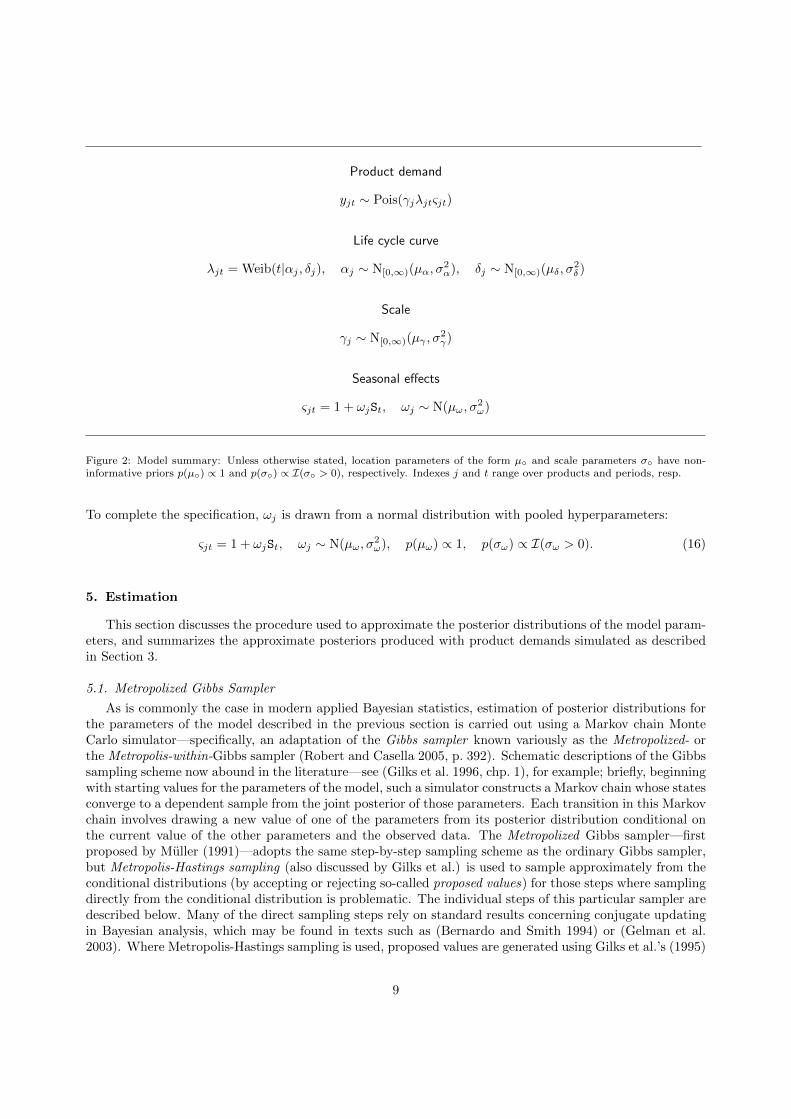
Product demand

yjt ∼ Pois(γjλjtςjt)

Life cycle curve

λjt = Weib(t|αj , δj), αj ∼ N[0,∞)(µα, σ2α), δj ∼ N[0,∞)(µδ, σ

2δ )

Scale

γj ∼ N[0,∞)(µγ , σ2γ)

Seasonal effects

ςjt = 1 + ωjSt, ωj ∼ N(µω, σ2ω)

Figure 2: Model summary: Unless otherwise stated, location parameters of the form µ◦ and scale parameters σ◦ have non-informative priors p(µ◦) ∝ 1 and p(σ◦) ∝ I(σ◦ > 0), respectively. Indexes j and t range over products and periods, resp.

To complete the specification, ωj is drawn from a normal distribution with pooled hyperparameters:

ςjt = 1 + ωjSt, ωj ∼ N(µω, σ2ω), p(µω) ∝ 1, p(σω) ∝ I(σω > 0). (16)

5. Estimation

This section discusses the procedure used to approximate the posterior distributions of the model param-eters, and summarizes the approximate posteriors produced with product demands simulated as describedin Section 3.

5.1. Metropolized Gibbs Sampler

As is commonly the case in modern applied Bayesian statistics, estimation of posterior distributions forthe parameters of the model described in the previous section is carried out using a Markov chain MonteCarlo simulator—specifically, an adaptation of the Gibbs sampler known variously as the Metropolized- orthe Metropolis-within-Gibbs sampler (Robert and Casella 2005, p. 392). Schematic descriptions of the Gibbssampling scheme now abound in the literature—see (Gilks et al. 1996, chp. 1), for example; briefly, beginningwith starting values for the parameters of the model, such a simulator constructs a Markov chain whose statesconverge to a dependent sample from the joint posterior of those parameters. Each transition in this Markovchain involves drawing a new value of one of the parameters from its posterior distribution conditional onthe current value of the other parameters and the observed data. The Metropolized Gibbs sampler—firstproposed by Muller (1991)—adopts the same step-by-step sampling scheme as the ordinary Gibbs sampler,but Metropolis-Hastings sampling (also discussed by Gilks et al.) is used to sample approximately from theconditional distributions (by accepting or rejecting so-called proposed values) for those steps where samplingdirectly from the conditional distribution is problematic. The individual steps of this particular sampler aredescribed below. Many of the direct sampling steps rely on standard results concerning conjugate updatingin Bayesian analysis, which may be found in texts such as (Bernardo and Smith 1994) or (Gelman et al.2003). Where Metropolis-Hastings sampling is used, proposed values are generated using Gilks et al.’s (1995)

9

adaptive rejection Metropolis sampling (ARMS) procedure, as implemented in the R package dlm (Petris2010).

In the following, each step is introduced by the conditional distribution from which a sample is tobe drawn. Variables of which the sampled quantity is conditionally independent are omitted from theconditioning set. In the interests of brevity, draws are specified only for αj and σα; samples for δj and σδare generated in an analogous manner. We abbreviate yj = (yj1, . . . , yjTj ).

γj∣∣ yj , αj , δj , µγ , σγ , ωj

The kernel of the full conditional distribution is given by the expression: Tj∏t=1

Pois(yjt|γjλjtςjt)

×N[0,∞)(γj |µγ , σ2γ),

where λjt and ςjt are the quantities determined by αj , δj and ωj in equation (13) and equation (16)resp. Sampling is carried out using the ARMS procedure.

αj∣∣ yj , γj , δj , µα, σα, ωj

The full conditional is proportional to the expression: Tj∏t=1

Pois(yjt|γjλjtςjt)

×N[0,∞)(αj |µα, σ2α).

This is also sampled using ARMS.

µα∣∣ α1, . . . , αJ , σα

Sampling is carried out using a device due to Griffiths (2004): Specifically, for l ∈ 1, . . . , J , let:

αl = µα + σα Φ−1

Φ(αl−µασα

)− Φ

(−µασα

)1− Φ

(−µασα

) , (17)

where Φ(·) denotes the standard normal cumulative distribution function.

Then as Griffiths demonstrates, supposing that αl ∼ N(µα, σ2α) and drawing from the conditional

distribution µα∣∣ α1, . . . , αJ , σα (a straightforward application of semi-conjugate updating with a non-

informative prior) is equivalent to drawing from µα∣∣ α1, . . . , αJ , σα given that αl ∼ N[0,∞)(µα, σ

2α).

σα∣∣ α1, . . . , αJ , µα

Again, using Griffiths’s device, draw from σα∣∣ α1, . . . , αJ , given that αj ∼ N(µα, σ

2α), where αj is

defined in equation (17).

ωj∣∣ yj , γj , αj , δj , µω, σω

Another ARMS step, with kernel: Tj∏t=1

Pois(yjt|γjλjt[1 + ωjSt])

×N(ωj |µω,σω2).

10

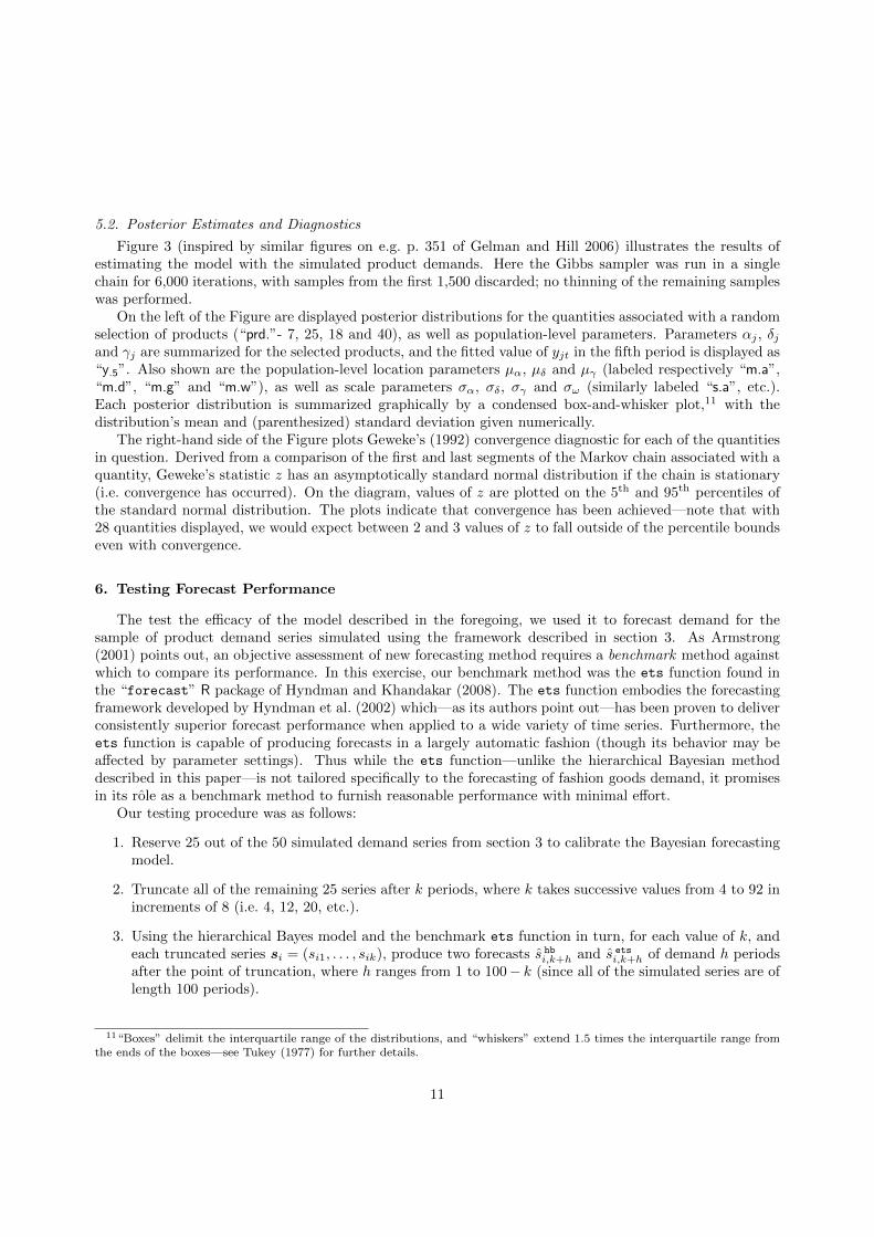
5.2. Posterior Estimates and Diagnostics

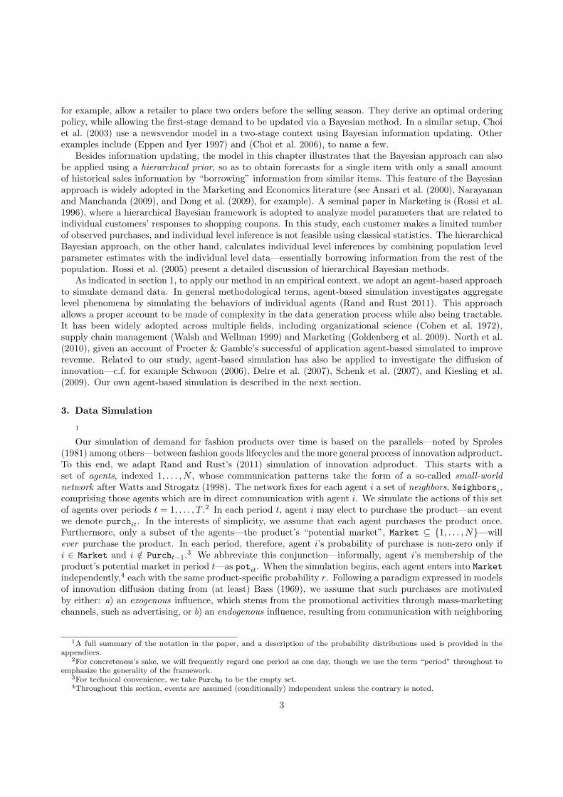
Figure 3 (inspired by similar figures on e.g. p. 351 of Gelman and Hill 2006) illustrates the results ofestimating the model with the simulated product demands. Here the Gibbs sampler was run in a singlechain for 6,000 iterations, with samples from the first 1,500 discarded; no thinning of the remaining sampleswas performed.

On the left of the Figure are displayed posterior distributions for the quantities associated with a randomselection of products (“prd.”- 7, 25, 18 and 40), as well as population-level parameters. Parameters αj , δjand γj are summarized for the selected products, and the fitted value of yjt in the fifth period is displayed as“y.5”. Also shown are the population-level location parameters µα, µδ and µγ (labeled respectively “m.a”,“m.d”, “m.g” and “m.w”), as well as scale parameters σα, σδ, σγ and σω (similarly labeled “s.a”, etc.).Each posterior distribution is summarized graphically by a condensed box-and-whisker plot,11 with thedistribution’s mean and (parenthesized) standard deviation given numerically.

The right-hand side of the Figure plots Geweke’s (1992) convergence diagnostic for each of the quantitiesin question. Derived from a comparison of the first and last segments of the Markov chain associated with aquantity, Geweke’s statistic z has an asymptotically standard normal distribution if the chain is stationary(i.e. convergence has occurred). On the diagram, values of z are plotted on the 5th and 95th percentiles ofthe standard normal distribution. The plots indicate that convergence has been achieved—note that with28 quantities displayed, we would expect between 2 and 3 values of z to fall outside of the percentile boundseven with convergence.

6. Testing Forecast Performance

The test the efficacy of the model described in the foregoing, we used it to forecast demand for thesample of product demand series simulated using the framework described in section 3. As Armstrong(2001) points out, an objective assessment of new forecasting method requires a benchmark method againstwhich to compare its performance. In this exercise, our benchmark method was the ets function found inthe “forecast” R package of Hyndman and Khandakar (2008). The ets function embodies the forecastingframework developed by Hyndman et al. (2002) which—as its authors point out—has been proven to deliverconsistently superior forecast performance when applied to a wide variety of time series. Furthermore, theets function is capable of producing forecasts in a largely automatic fashion (though its behavior may beaffected by parameter settings). Thus while the ets function—unlike the hierarchical Bayesian methoddescribed in this paper—is not tailored specifically to the forecasting of fashion goods demand, it promisesin its role as a benchmark method to furnish reasonable performance with minimal effort.

Our testing procedure was as follows:

1. Reserve 25 out of the 50 simulated demand series from section 3 to calibrate the Bayesian forecastingmodel.

2. Truncate all of the remaining 25 series after k periods, where k takes successive values from 4 to 92 inincrements of 8 (i.e. 4, 12, 20, etc.).

3. Using the hierarchical Bayes model and the benchmark ets function in turn, for each value of k, andeach truncated series si = (si1, . . . , sik), produce two forecasts s hb

i,k+h and s etsi,k+h of demand h periods

after the point of truncation, where h ranges from 1 to 100− k (since all of the simulated series are oflength 100 periods).

11“Boxes” delimit the interquartile range of the distributions, and “whiskers” extend 1.5 times the interquartile range fromthe ends of the boxes—see Tukey (1977) for further details.

11

Posterior distribution Convergence

α

prd.40prd.18prd.25prd.7

20 30 40 50 60 70

60 (0.89) 14 (0.36) 71 (0.85) 11 (0.36)

−1.27 [0.20]0.05 [0.96]−0.98 [0.33]0.08 [0.93]

●

●

●

●

δ

prd.40prd.18prd.25prd.7

110 120 130 140

1.2e+02 (2.8)1.2e+02 (2.6)1.1e+02 ( 2)1.3e+02 (3.6)

0.77 [0.44]0.13 [0.89]0.48 [0.63]−0.34 [0.74]

●

●

●

●

γ

prd.40prd.18prd.25prd.7

2600 2800 3000 3200 3400 3600 3800

2.7e+03 ( 51)3.8e+03 ( 61)2.6e+03 ( 51)3.6e+03 ( 61)

1.45 [0.15]0.05 [0.96]0.63 [0.53]0.08 [0.94]

●

●

●

●

ω

prd.40prd.18prd.25prd.7

0.48 0.49 0.50 0.51 0.52 0.53 0.54

0.51 (0.015)0.5 (0.015)0.51 (0.015)0.51 (0.015)

0.36 [0.72]−0.02 [0.98]0.58 [0.56]0.48 [0.63]

●

●

●

●

y5

prd.40prd.18prd.25prd.7

0 20 40 60 80

0.92 (0.96) 56 (7.7)0.18 (0.42) 64 (8.1)

0.97 [0.33]0.31 [0.75]−1.53 [0.13]−0.11 [0.91]

●

●

●

●

α, δ

m.as.a

m.ds.d

20 40 60 80 100 120 140

23 (4.2) 24 (2.7)1.4e+02 (2.8) 19 (2.1)

−0.22 [0.83]0.31 [0.76]−0.75 [0.45]0.60 [0.55]

●

●

●

●

γ

m.gs.g

500 1000 1500 2000 2500 3000

3.1e+03 ( 77)5.4e+02 ( 56)

−0.36 [0.72]2.54 [0.01]

●

●

ω

m.ws.w

0.1 0.2 0.3 0.4 0.5

0.5 (0.0095)0.0091 (0.0078)

0.10 [0.92]0.72 [0.47]

●

●

Figure 3: Posterior distributions and convergence diagnostics for model fit to full sample of simulated demand series: On theleft are interquartile ranges and 1.5×interquartile ranges of quantities associated with selected products (prd.-) and hyperpa-rameters, together with the mean and standard deviation of the corresponding distribution. On the right are values of Geweke’sconvergence statistic; all but one of the values lie between the 5th and 95th percentiles of the standard normal distribution(statistic values and p-values appear on the far right), so convergence is reasonably assured.

12

Forecasting with the Bayesian model involves subjecting both the 25 reserved demand series as wellthe 25 truncated series to the procedure set out in Section 4.1, using the MCMC simulator describedin Section 5.1 to produce a sample from the posterior predictive distribution for si,k+h, and taking themedian of this sample as the point forecast.

The ets function did not use the calibration series, but we found that to produce reasonable forecastswith the function at longer horizons (i.e. h in excess of 20 or so), it was necessary to provide some hintsto its automatic model selection algorithm, constraining it to look for models with damped, additivetrends (Gardner and McKenzie 1989, Hyndman et al. 2002).

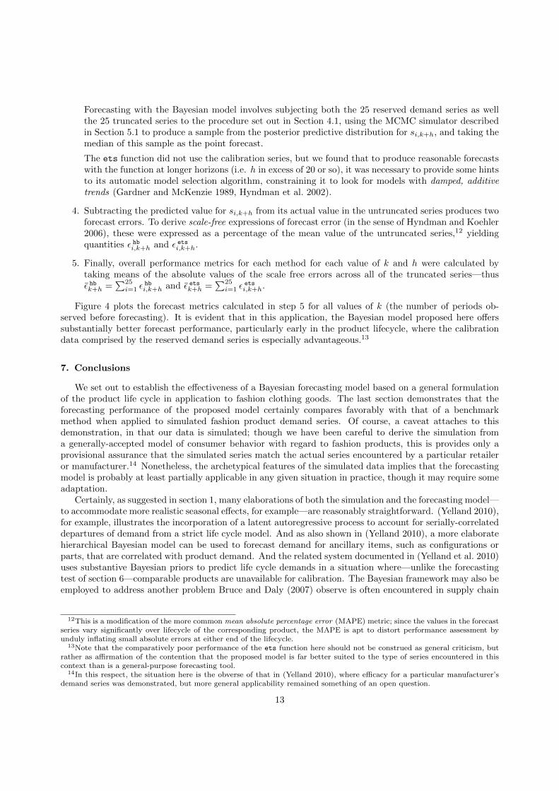
4. Subtracting the predicted value for si,k+h from its actual value in the untruncated series produces twoforecast errors. To derive scale-free expressions of forecast error (in the sense of Hyndman and Koehler2006), these were expressed as a percentage of the mean value of the untruncated series,12 yieldingquantities ε hbi,k+h and ε etsi,k+h.

5. Finally, overall performance metrics for each method for each value of k and h were calculated bytaking means of the absolute values of the scale free errors across all of the truncated series—thusε hbk+h =

∑25i=1 ε

hbi,k+h and ε etsk+h =

∑25i=1 ε

etsi,k+h.

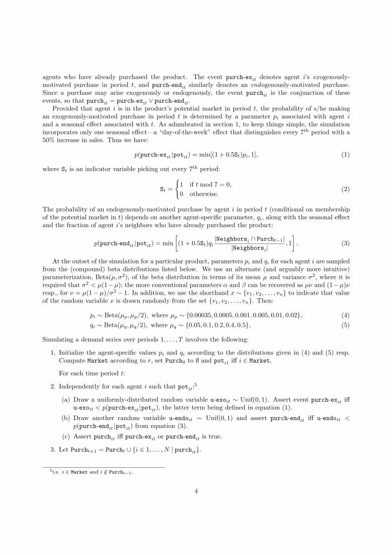
Figure 4 plots the forecast metrics calculated in step 5 for all values of k (the number of periods ob-served before forecasting). It is evident that in this application, the Bayesian model proposed here offerssubstantially better forecast performance, particularly early in the product lifecycle, where the calibrationdata comprised by the reserved demand series is especially advantageous.13

7. Conclusions

We set out to establish the effectiveness of a Bayesian forecasting model based on a general formulationof the product life cycle in application to fashion clothing goods. The last section demonstrates that theforecasting performance of the proposed model certainly compares favorably with that of a benchmarkmethod when applied to simulated fashion product demand series. Of course, a caveat attaches to thisdemonstration, in that our data is simulated; though we have been careful to derive the simulation froma generally-accepted model of consumer behavior with regard to fashion products, this is provides only aprovisional assurance that the simulated series match the actual series encountered by a particular retaileror manufacturer.14 Nonetheless, the archetypical features of the simulated data implies that the forecastingmodel is probably at least partially applicable in any given situation in practice, though it may require someadaptation.

Certainly, as suggested in section 1, many elaborations of both the simulation and the forecasting model—to accommodate more realistic seasonal effects, for example—are reasonably straightforward. (Yelland 2010),for example, illustrates the incorporation of a latent autoregressive process to account for serially-correlateddepartures of demand from a strict life cycle model. And as also shown in (Yelland 2010), a more elaboratehierarchical Bayesian model can be used to forecast demand for ancillary items, such as configurations orparts, that are correlated with product demand. And the related system documented in (Yelland et al. 2010)uses substantive Bayesian priors to predict life cycle demands in a situation where—unlike the forecastingtest of section 6—comparable products are unavailable for calibration. The Bayesian framework may also beemployed to address another problem Bruce and Daly (2007) observe is often encountered in supply chain

12This is a modification of the more common mean absolute percentage error (MAPE) metric; since the values in the forecastseries vary significantly over lifecycle of the corresponding product, the MAPE is apt to distort performance assessment byunduly inflating small absolute errors at either end of the lifecycle.

13Note that the comparatively poor performance of the ets function here should not be construed as general criticism, butrather as affirmation of the contention that the proposed model is far better suited to the type of series encountered in thiscontext than is a general-purpose forecasting tool.

14In this respect, the situation here is the obverse of that in (Yelland 2010), where efficacy for a particular manufacturer’sdemand series was demonstrated, but more general applicability remained something of an open question.

13

Forecast period

Me

an

sca

led

ab

s. e

rro

r (%

), ε

k+h, fo

r p

eri

od

0

100

200

300

400

0 20 40 60 80 100

Known periods, k = 4 k = 12

0 20 40 60 80 100

k = 20 k = 28

k = 36 k = 44 k = 52

0

100

200

300

400

k = 60

0

100

200

300

400

k = 68

0 20 40 60 80 100

k = 76 k = 84

0 20 40 60 80 100

k = 92

Hierarchical Bayes model, hb Package 'forecast' function, ets

Figure 4: Forecast performance of the model and benchmark.

14

management for fashion retailing, viz., the availability of timely sales data that is only approximate and/orprovisional. With a Bayesian model, revised forecasts can be produced by treating early sales data as softevidence, known only with uncertainty—see e.g. (Pearl 1988, Valtorta et al. 2002, Pan et al. 2006) for detailsof methods for updating Bayesian models with soft evidence.

With regard to applying our work in an industry setting, as we suggest in section 1, recent developmentsin the fashion industry are highly favorable to a life cycle based Bayesian model such as the one describedhere: First, as Hines and Bruce (2007) indicate, increasing globalization of the industry—driven by thedismantling of tarrif barriers, improvements in transportation and communication technology, competitivepressures militating in favor of low-cost off-shore manufacturing and the rise of geographically-disperseddesign and manufacturing hubs in Europe and the Far East—has made relatively long lead times a realityin many sectors of the industry. Effectively addressing such lead times necessitates relatively long-termforecasts, in which product life cycles are frequently a significant factor. Second, as competitive pressuresaccelerate the trend towards “fast fashion” and “quick response” (Kang 1999) even in low-cost retail lines,updates to forecasts prior to and during the selling season are becoming the norm;15 Bayesian forecastingof the sort demonstrated here is perfectly suited to producing such updates. We would also be interestedin establishing the broader viability of the use of agent-based simulation models as a means of calibratingthe efficacy of different forecasting models a priori. Agent-based simulation is already a proven approachto operations planning for supply chains (see (Fox et al. 2000), for example), but to our knowledge, the useof agent-based simulation to compare forecasting models is an area of research still to be explored. Withits continuing protean changes in sourcing and retailing arrangements, the fashion industry constitutes anideal venue for such work.

References

N. Agrawal and S. A. Smith. Estimating negative binomial demand for retail inventory management withunobservable lost sales. Naval Research Logistics, 43(6):839–861, 1996.

A. Ansari, K. Jedidi, and S. Jagpal. A hierarchical Bayesian methodology for treating heterogeneity instructural equation models. Marketing Science, 19(4):328–347, 2000.

J. M. Armstrong. Standards and practices for forecasting. In J. M. Armstrong, editor, Principles ofForecasting: A Handbook for Researchers and Practitioners, pages 171–192. Kluwer, Norwell, MA, 2001.

K. S. Azoury. Bayesian solution to dynamic inventory models under unknown demand distribution. Man-agement Science, 31:1150–1160, 1985.

K. S. Azoury and B. S. Miller. A comparison of the optimal levels of Bayesian and non-Bayesian inventorymodels. Management Science, 30:993–1003, 1984.

F. Bass. A new product growth model for consumer durables. Management Science, 15:215–227, 1969.

J. M. Bernardo and A. F. M. Smith. Bayesian Theory. Wiley, Hoboken, NJ, 1994.

P. J. Brockwell and R. A. Davis. Introduction to Time Series and Forecasting. Springer, 2nd edition, 2002.

M. Bruce and L. Daly. Challenges of fashion buying and merchandising. In T. Hines and M. Bruce, editors,Fashion Marketing: Contemporary Issues, chapter 3, pages 54–69. Elsevier, 2nd edition, 2007.

F. Caro and J. Gallien. Dynamic assortment with demand learning for seasonal consumer goods. Manage-ment Science, 53(2):276–292, 2007.

T. M. Choi, D. Li, and H. M. Yan. Optimal two-stage ordering policy with Bayesian information updating.Journal of the Operational Research Society, 54(8):846–859, 2003.

T. M. Choi, D. Li, and H. M. Yan. Quick response policy with Bayesian information updates. EuropeanJournal of Operational Research, 170(3):788–808, 2006.

15Hines and Bruce (2007) point out that “fast fashion” retailers such as Zara and Primark publish revised forecasts on aweekly basis.

15

M. D. Cohen, J. G. March, and J. P. Olsen. A garbage can model of organizational choice. AdministrativeScience Quarterly, 17:1–25, 1972.

S. R. Cook, A. Gelman, and D. B. Rubin. Validation of software for Bayesian models using posteior quantiles.Journal of Computational and Graphical Statistics, 15(3):675–692, 2006.

S. A. Delre, W. Jager, T. H. A. Bijmolt, and M. A. Janssen. Targeting and timing promotional activities:An agent-based model for the takeoff of new products. Journal of Business Research, 60(8):826–835, 2007.

X. Dong, P. Manchanda, and P. K. Chintagunta. Quantifying the benefits of individual-level targeting inthe presence of firm strategic behavior. Journal of Marketing Research, 9(3):301–337, 2009.

K. L. Donohue. Efficient supply contracts for fashion goods with forecast updating and two productionmodes. Management Science, 46(11):1397–1411, 2000.

A. Dvoretzky, J. Kiefer, and J. Wolfowitz. The inventory problem: Case of known distribution of demand.Econometrica, 20:187–222, 1952.

G. D. Eppen and A. V. Iyer. Improved fashion buying with Bayesian updating. Operations Research, 45(6):805–819, 1997.

M. S. Fox, M. Barbuceanu, and R. Teigen. Agent-oriented supply-chain management. Intl. Journal ofFlexible Manufacturing Systems, 12:165–188, 2000.

E. S. Gardner and E. McKenzie. Seasonal exponential smoothing with damped trends. Management Science,35(3):372–376, March 1989.

A. Gelman. Prior distributions for variance parameters in hierarchical models. Bayesian Analysis, 1(3):515–533, 2006.

A. Gelman and J. Hill. Data Analysis Using Regression and Multilevel/Hierarchical Models. CambridgeUniversity Press, New York, 2006.

A. Gelman, J. Carlin, H. Stern, and D. Rubin. Bayesian Data Analysis. Chapman & Hall/CRC Press, BocaRaton, FL, 2nd edition, 2003.

J. Geweke. Evaluating the accuracy of sampling-based approaches to calculating posterior moments. InJ. M. Bernardo, J. O. Berger, A. P. Dawid, and A. F. M. Smith, editors, Bayesian Statistics, volume 4,pages 169–193. Clarendon Press, Wotton-under-Edge, Gloucestershire, UK, 1992.

W. R. Gilks, N. G. Best, and K. K. C. Tan. Adaptive rejection Metropolis sampling within Gibbs sampling.Applied Statistics, 44:455–472, 1995. (Corr: Neal, R.M. 1997 v.46 pp.541-542).

W. R. Gilks, S. Richardson, and D. J. Spiegelhalter. Markov Chain Monte Carlo in Practice. Chapman &Hall, Boca Raton, FL, 1996.

J. Goldenberg, S. Han, D. R. Lehmann, and J. W. Hong. The role of hubs in the adoption process. Journalof Marketing, 73(2):1–13, 2009.

W. Griffiths. A Gibbs sampler for the parameters of a truncated multivariate normal distribution. InR. Becker and S. Hum, editors, Contemporary Issues in Economics and Econometrics: Theory and Ap-plication, pages 75–91. Edward Elgar, 2004.

H. Gurnani and C.S. Tang. Note: Optimal ordering decisions with uncertain cost and demand forecastupdating. Management Science, 45(10):1456–1462, 1999.

A. C. Harvey. Forecasting, Structural Time Series Models and the Kalman Filter. Cambridge UniversityPress, Cambridge, UK, 1989.

T. Hines and M. Bruce. Fashion Marketing. Elsevier, Oxford, 2007.

N. A. Hunter and P. Valentino. Quick response—ten years later. International Journal of Clothing Scienceand Technology, 7:30–40, 1995.

R. J. Hyndman and Y. Khandakar. Automatic time series forecasting: The forecast package for R. Journalof Statistical Software, 27(3):1–22, July 2008. URL http://www.jstatsoft.org/v27/i03.

R. J. Hyndman and A. B. Koehler. Another look at measures of forecast accuracy. International Journal

16

of Forecasting, 22:679–688, 2006.

R. J. Hyndman, A. B. Koehler, R. D. Snyder, and S. Grose. A state space framework for automaticforecasting using exponential smoothing methods. International Journal of Forecasting, 18(3):439–454,2002.

D. Iglehart. The dynamic inventory problem with unknown demand distribution. Management Science, 10:429–440, 1964.

A. Iyer and M. E. Bergen. Quick response in manufacturer-retailer channels. Management Science, 43(4):559–570, 1997.

K.-Y. Kang. Development of an Assortment-Planning Model for Fashion-Sensitive Products. PhD thesis,Virginia Polytechnic Institute and State University, 1999.

E. Kiesling, M. Gunther, C. Stummer, and L .M. Wakolbinger. An agent-based simulation model for themarket diffusion of a second generation biofuel. In Winter Simulation Conference, 2009.

K. Krishnamoorthy. Handbook of Statistical Distributions with Applications. Statistics: A Series of Textbooksand Monographs. Chapman and Hall/CRC, 2006.

V. Mahajan, E. Muller, and Y. Wind, editors. New-Product Diffusion Models. Kluwer, Norwell, MA, 2000.

J. I. McCool. Using the Weibull Distribution: Reliability, Modeling, and Inference. Wiley, 2012.

B. Miller. Scarf’s state reduction method, flexibility and a dependent demand inventory model. OperationsResearch, 34(1):83–90, 1986.

W. W. Moe and P. S. Fader. Using advance purchase orders to forecast new product sales. MarketingScience, 21(3):347–364, Summer 2002.

P. Muller. A generic approach to posterior integration and Gibbs sampling. Technical Report 91-09,Department of Statistics, Purdue University, 1991.

G. R Murray, Jr. and E. A. Silver. A Bayesian analysis of the style goods inventory problem. ManagementScience, 12(11):785–797, 1966.

S. Narayanan and P. Manchanda. Heterogeneous learning and the targeting of marketing communicationfor new products. Marketing Science, 28(3):424–441, 2009.

M. J. North, C. M. Macal, J. St. Aubin, P. Thimmapuram, M. Bragen, and J. Hahn. Multi-scale agent-basedconsumer market modeling. Complexity, 15(5):37–47, 2010.

R. Pan, Y. Peng, and Z. Ding. Belief update in bayesian networks using uncertain evidence. In Intl. Conf.on Tools with Artificial Intelligence, ICTAI, pages 441–444, 2006.

J. Pearl. Probabilistic Reasoning in Intelligent Systems: Networks of Plausible Inference. Morgan Kaufmann,1988.

G. Petris. dlm: Bayesian and likelihood analysis of dynamic linear models, 2010. URL http://cran.r-project.org/web/packages/dlm/index.html.

W. Rand and R. T. Rust. Agent-based modeling in marketing: Guidelines for rigor. International Journalof Research in Marketing, 28(3):181–183, September 2011.

C. P. Robert and G. Casella. Monte Carlo Statistical Methods. Springer, New York, 2nd edition, 2005.

P. E. Rossi, R. E. McCulloch, and G. M. Allenby. The value of purchase history data in target marketing.Marketing Science, 15(4):321–340, 1996.

P. E. Rossi, G. M. Allenby, and R. E. McCulloch. Bayesian Statistics and Marketing. Wiley, 2005.

H. Scarf. Bayes solutions of the statistical inventory problem. Annals of Mathematical Statistics, 30(2):490–508, 1959.

T. A. Schenk, G. Loffler, and J. Rauh. Agent-based simulation of consumer behavior in grocery shoppingon a regional level. Journal of Business Research, 60(8):894–903, 2007.

M. Schwoon. Simulating the adoption of fuel cell vehicles. Journal of Evolutionary Economics, 16(4):435–472, 2006.

17

M. N. Sharif and M. N. Islam. The Weibull distribution as a general model for forecasting technologicalchange. Technological Forecasting and Social Change, 18:247–256, 1980.

G. B. Sproles. Analyzing fashion life cycles: Principles and perspectives. Journal of Marketing, 45:116–124,1981.

J.W. Tukey. Exploratory Data Analysis. Addison-Wesley, 1977.

M. Valtorta, K. Young-Gyun, and J. Vomlel. Soft evidential update for probabilistic multiagent systems.Intl. Journal of Approximate Reasoning, 29:71–106, 2002.

W. Walsh and M. Wellman. Modeling supply chains formation in multi-agent systems. In IJCAI-99 Work-shop Agent-Mediated Electronic Commerce, 1999.

D. J. Watts and S. H. Strogatz. Collective dynamics of ‘small-world’ networks. Nature, 393:409–410, 1998.

D. S. Wu, K. G. Kempf, M. O. Atan, B. Aytac, S. A. Shirodkar, and A. Mishra. Improving new productforecasting at Intel corporation. Interfaces, 40(5):385–396, 2010.

P. M. Yelland. Bayesian forecasting of parts demand. International Journal of Forecasting, 26(2):374–396,April–June 2010.

P. M. Yelland, S. Kim, and R. Stratulate. A Bayesian model for sales forecasting at Sun Microsystems.Interfaces, 2010.

18

Appendices

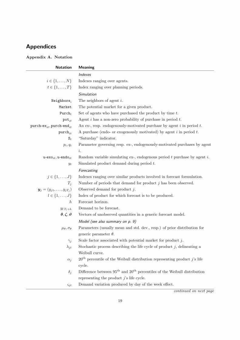
Appendix A. Notation

Notation Meaning

Indexes

i ∈ {1, . . . , N} Indexes ranging over agents.

t ∈ {1, . . . , T} Index ranging over planning periods.

Simulation

Neighborsi The neighbors of agent i.

Market The potential market for a given product.

Purcht Set of agents who have purchased the product by time t.

potit Agent i has a non-zero probability of purchase in period t.

purch-exit, purch-endit An ex-, resp. endogenously-motivated purchase by agent i in period t.

purchit A purchase (endo- or exogenously motivated) by agent i in period t.

St “Saturday” indicator.

pi, qi Parameter governing resp. ex-, endogenously-motivated purchases by agent

i.

u-exoit, u-endoit Random variable simulating ex-, endogenous period t purchase by agent i.

yt Simulated product demand during period t.

Forecasting

j ∈ {1, . . . , J} Indexes ranging over similar products involved in forecast formulation.

Tj Number of periods that demand for product j has been observed.

yj = (yj1, . . . , yjTj ) Observed demand for product j.

l ∈ {1, . . . , J} Index of product for which forecast is to be produced.

h Forecast horizon.

yl Tl+h Demand to be forecast.

θ, ζ,ϑ Vectors of unobserved quantities in a generic forecast model.

Model (see also summary on p. 9)

µθ, σθ Parameters (usually mean and std. dev., resp.) of prior distribution for

generic parameter θ.

γj Scale factor associated with potential market for product j.

λjt Stochastic process describing the life cycle of product j, delineating a

Weibull curve.

αj 20th percentile of the Weibull distribution representing product j’s life

cycle.

δj Difference between 95th and 20th percentiles of the Weibull distribution

representing the product j’s life cycle.

ςjt Demand variation produced by day of the week effect.

continued on next page

19

Notation Meaning

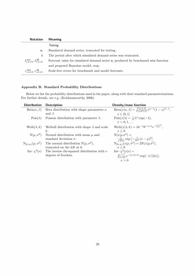
Testing

si Simulated demand series, truncated for testing.

k The period after which simulated demand series was truncated.

s etsi,k+h, s

hbi,k+h Forecast value for simulated demand series si produced by benchmark ets function

and proposed Bayesian model, resp.

ε etsi,k+h, εhbi,k+h Scale-free errors for benchmark and model forecasts.

Appendix B. Standard Probability Distributions

Below we list the probability distributions used in the paper, along with their standard parameterizations.For further details, see e.g. (Krishnamoorthy 2006).

Distribution Description Density/mass function

Beta(α, β) Beta distribution with shape parameters αand β.

Beta(x|α, β) = Γ(α+β)Γ(α)Γ(β)x

α−1(1− x)β−1,

x ∈ [0, 1]Pois(λ) Poisson distribution with parameter λ. Pois(x|λ) = 1

x!λx exp(−λ),

x = 0, 1, . . .

Weib(λ, k) Weibull distribution with shape λ and scalek.

Weib(x|λ, k) = λk−λθ−1+λe−( θk )λ

,x ≥ 0

N(µ, σ2) Normal distribution with mean µ andstandard deviation σ.

N(x|µ,σ2) =1√2πσ

exp[− 1

2σ2 (x− µ)2]

N[0,∞)(µ, σ2) The normal distribution N(µ, σ2),

truncated on the left at 0.N[0,∞)(x|µ, σ2) = 2N(x|µ,σ2),x ≥ 0

Inv–χ2(ν) The inverse chi-squared distribution with νdegrees of freedom.

Inv–χ2(x|ν) =2−ν/2

Γ(ν/2)x−(ν/2+1) exp[−1/(2x)],

x > 0

20