9781461448686-c1

Chapter 2Probability Distances and Probability Metrics:Definitions

The goals of this chapter are to:

• Provide examples of metrics in probability theory;• Introduce formally the notions of a probability metric and a probability distance;• Consider the general setting of random variables (RVs) defined on a given

probability space .�;A; Pr/ that can take values in a separable metric space U

in order to allow for a unified treatment of problems involving random elementsof a general nature;

• Consider the alternative setting of probability distances on the space of proba-bility measures P2 defined on the �-algebras of Borel subsets of U 2 D U � U ,where U is a separable metric space;

• Examine the equivalence of the notion of a probability distance on the space ofprobability measures P2 and on the space of joint distributions LX2 generated bypairs of RVs .X; Y / taking values in a separable metric space U .

S.T. Rachev et al., The Methods of Distances in the Theory of Probability and Statistics,DOI 10.1007/978-1-4614-4869-3 2, © Springer Science+Business Media, LLC 2013

11

12 2 Probability Distances and Probability Metrics: Definitions

Notation introduced in this chapter:

Notation Description

EN Engineer’s metricXp Space of real-valued random variables with EjX jp < 1� Uniform (Kolmogorov) metricX D X.R/ Space of real-valued random variablesL Levy metric� Kantorovich metric�p Lp -metric between distribution functionsK, K� Ky Fan metricsLp Lp -metric between random variablesMOMp Metric between pth moments.S; �/ Metric space with metric �

Rn n-dimensional vector space

r.C1; C2/ Hausdorff metric (semimetric between sets)s.F; G/ Skorokhod metricK D K� Parameter of a distance spaceH Class of Orlicz’s functions�H Birnbaum–Orlicz distanceKr Kruglov distance.U; d/ Separable metric space with metric d

s.m.s. Separable metric spaceU k k-fold Cartesian product of U

Bk D Bk.U / Borel � -algebra on U k

Pk D Pk.U / Space of probability laws on Bk

T˛;ˇ;:::;� P Marginal of P 2 Pk on coordinates ˛, ˇ, : : :, �

PrX Distribution of X

� Probability semidistanceX WD X.U / Set of U -valued RVsLX2 WD LX2.U / Space of PrX;Y , X; Y 2 X.U /

u.m. Universally measurableu.m.s.m.s. Universally measurable separable metric space

2.1 Introduction

Generally speaking, a functional that measures the distance between randomquantities is called a probability metric.1 In this chapter, we provide differentexamples of probability metrics and discuss an application of the Kolmogorov

1Mostafaei and Kordnourie (2011) is a more recent general publication on probability metrics andtheir applications.

2.2 Examples of Metrics in Probability Theory 13

metric in mathematical statistics. Then we proceed with the axiomatic constructionof probability metrics on the space of probability measures defined on the twofoldCartesian product of a separable metric space U . This definition induces byrestriction a probability metric on the space of joint distributions of random elementsdefined on a probability space .�;A; Pr/ and taking values in the space U . Finally,we demonstrate that under some fairly general conditions, the two constructions areessentially the same.

2.2 Examples of Metrics in Probability Theory

Below is a list of various metrics commonly found in probability and statistics.

1. Engineer’s metric:

EN.X; Y / WD jE.X/ � E.Y /j; X; Y 2 X1; (2.2.1)

where Xp is the space of all real-valued RVs) with EjX jp < 1.2. Uniform (or Kolmogorov) metric:

�.X; Y / WD supfjFX.x/ � FY .x/j W x 2 Rg; X; Y 2 X D X.R/; (2.2.2)

where FX is the distribution function (DF) of X , R D .�1; C1/, and X is thespace of all real-valued RVs.

3. Levy metric:

L.X; Y / WD inff" > 0 W FX .x � "/ � " � FY .x/ � FX .x C "/ C "; 8x 2 Rg:(2.2.3)

Remark 2.2.1. We see that � and L may actually be considered metrics on thespace of all distribution functions. However, this cannot be done for EN simplybecause EN.X; Y / D 0 does not imply the coincidence of FX and FY , while�.X; Y / D 0 ” L.X; Y / D 0 ” FX D FY . The Levy metric metrizesweak convergence (convergence in distribution) in the space F , whereas � is oftenapplied in the central limit theorem (CLT).2

4. Kantorovich metric:

�.X; Y / DZR

jFX .x/ � FY .x/jdx; X; Y 2 X1:

2See Hennequin and Tortrat (1965).


5. Lp-metrics between distribution functions:

�p.X; Y / WD�Z 1

�1jFX.t/ � FY .t/jpdt

�1=p

; p � 1; X; Y 2 X1: (2.2.4)

Remark 2.2.2. Clearly, � D �1. Moreover, we can extend the definition of �p whenp D 1 by setting �1 D �. One reason for this extension is the following dualrepresentation for 1 � p � 1:

�p.X; Y / D supf 2Fp

jEf .X/ � Ef .Y /j; X; Y 2 X1;

where Fp is the class of all measurable functions f with kf kq < 1. Here,kf kq.1=p C 1=q D 1/ is defined, as usual, by3

kf kq WD

8ˆ<ˆ:

�Zjf jq

�1=q

; 1 � q < 1;

ess supR

jf j; q D 1:

6. Ky Fan metrics:

K.X; Y / WD inff" > 0 W Pr.jX � Y j > "/ < "g; X; Y 2 X; (2.2.5)

and

K�.X; Y / WD EjX � Y j

1 C jX � Y j : (2.2.6)

Both metrics metrize convergence in probability on X D X.R/, the space ofreal RVs.4

7. Lp-metric:

Lp.X; Y / WD fEjX � Y jpg1=p; p � 1; X; Y 2 Xp: (2.2.7)

Remark 2.2.3. Define

mp.X/ WD fEjX jpg1=p; p > 1; X 2 Xp: (2.2.8)

and

MOMp.X; Y / WD jmp.X/ � mp.Y /j; p � 1; X; Y 2 Xp: (2.2.9)

3The proof of this representation is given by (Dudley, 2002, p. 333) for the case p D 1.4See Lukacs (1968, Chap. 3) and Dudley (1976, Theorem 3.5).

2.3 Kolmogorov Metric: A Property and an Application 15

Then we have, for X0; X1; : : : 2 Xp,

Lp.Xn; X0/ ! 0 ”�

K.Xn; X0/ ! 0;

MOMp.Xn; X0/ ! 0(2.2.10)

[see, e.g., Lukacs (1968, Chap. 3)].

Other probability metrics in common use include the discrepancy metric,the Hellinger distance, the relative entropy metric, the separation distance metric, the�2-distance, and the f -divergence metric. These probability metrics are summa-rized in Gibbs and Su (2002).

All of the aforementioned (semi-)metrics on subsets of X may be divided intothree main groups: primary, simple, and compound (semi-)metrics. A metric � isprimary if �.X; Y / D 0 implies that certain moment characteristics of X and Y

agree. As examples, we have EN (2.2.1) and MOMp (2.2.9). For these metrics

EN.X; Y / D 0 ” EX D EY;

MOMp.X; Y / D 0 ” mp.X/ D mp.Y /: (2.2.11)

A metric � is simple if

�.X; Y / D 0 ” FX D FY : (2.2.12)

Examples are � (2.2.2), L (2.2.3), and �p (2.2.4). The third group, the compound(semi-)metrics, has the property

�.X; Y / D 0 ” Pr.X D Y / D 1: (2.2.13)

Some examples are K (2.2.5), K� (2.2.6), and Lp (2.2.7).Later on, precise definitions of these classes will be given as well as a study of

the relationships between them. Now we will begin with a common definition ofprobability metric that will include the types mentioned previously.

2.3 Kolmogorov Metric: A Property and an Application

In this section, we consider a paradoxical property of the Kolmogorov metric andan application in the area of mathematical statistics.

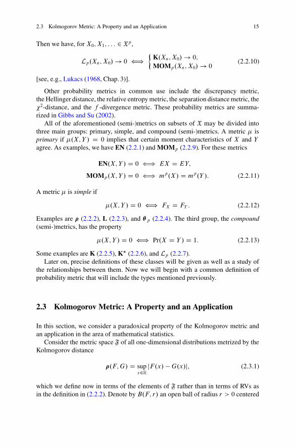
Consider the metric space F of all one-dimensional distributions metrized by theKolmogorov distance

�.F; G/ D supx2R

jF.x/ � G.x/j; (2.3.1)

which we define now in terms of the elements of F rather than in terms of RVs asin the definition in (2.2.2). Denote by B.F; r/ an open ball of radius r > 0 centered


−0.5 0 0.5 1 1.5−0.2

0

0.2

0.4

0.6

0.8

1

1.2Fig. 2.1 The ball B.Fo; ı˛/.The solid line is the center ofthe ball and the dashed linerepresents the boundary ofthe ball

at F in the metric space F with �-distance and let Fo be a continuous distributionfunction (DF). The following result holds.

Theorem 2.3.1. For any r > 0 there exists a continuous DF Fr such that

B.Fr ; r/ � B.Fo; r/ (2.3.2)

and

B.Fr ; r/ ¤ B.Fo; r/:

Proof. Let us show that there are Fo and Fa such that (2.3.2) holds. Without loss ofgenerality we may choose

Fo.x/ D

8<ˆ:

0; x < 0;

x; 0 � x < 1;

1; x � 1:

For a given (but fixed) n define ı˛ such that (2.3.1) is true.Figure 2.1 provides an illustration of the ball B.Fo; ı˛/. The boundary of the ball

is shown by means of a dashed line, the center of the ball is the solid line, and theradius ı˛ equals 0.2.

Consider now Fa defined in the following way:

Fa.x/ D

8ˆˆ<ˆˆ:

0; x < ı˛=2;

2x � ı˛; ı˛=2 � x < ı˛;

x; ı˛ � x < 1 � ı˛;

2x � .1 � ı˛/; 1 � ı˛ � x < 1 � ı˛=2;

1; x � 1 � ı˛=2:

2.3 Kolmogorov Metric: A Property and an Application 17

−0.5 0 0.5 1 1.5−0.2

0

0.2

0.4

0.6

0.8

1

1.2Fig. 2.2 The ball B.Fa; ı˛/.The solid line is the center ofthe ball and the dashed linerepresents the boundary ofthe ball

An illustration is given in Fig. 2.2. Comparing Figs. 2.1 and 2.2, we can see that

B.Fa; ı˛/ � B.Fo; ı˛/

andB.Fa; ı˛/ ¤ B.Fo; ı˛/: ut

We demonstrate that this property leads to biasedness of the Kolmogorovgoodness-of-fit tests. Suppose that X1; : : : ; Xn are independent and identicallydistributed (i.i.d.) RVs (observations) with (unknown) DF F . Based on the observa-tions, one needs to test the hypothesis

Ho W F D Fo;

where Fo is a fixed DF.

Definition 2.3.1. For a specific alternative hypothesis, a test is said to be unbiasedif the probability of rejecting the null hypothesis

(a) Is greater than or equal to the significance level ˛ when the alternative is trueand

(b) Is less than or equal to the significance level when the null hypothesis is true.

A test is said to be biased for an alternative hypothesis if it is not unbiased for thisalternative.

Let d be a distance in the space of all probability distributions on the real line.Below we consider a test with the following properties:

1. We reject the null hypothesis Ho if

d.Gn; Fo/ > ı˛;


where Gn is an empirical DF constructed on the basis of the observationsX1; : : : ; Xn and ı˛ satisfies

Prfd.Gn; Fo/ > ı˛g � ˛: (2.3.3)

2. The test is distribution free, i.e.,

PrF fd.Gn; Fo/ > ı˛g

does not depend on continuous DF F .

We refer to such tests as distance-based tests.

Theorem 2.3.2. Suppose that for some ˛ > 0 there exists a continuous DF Fa suchthat

B.Fa; ı˛/ � B.Fo; ı˛/ (2.3.4)

andPrFofGn 2 B.Fo; ı˛/ n B.Fa; ı˛/g > 0: (2.3.5)

Then the distance-based test is biased for the alternative Fa.

Proof. Let X1; : : : ; Xn be a sample from Fa and Gn be the corresponding empiricalDF. Then

PrFofGn 2 B.Fo; ı˛/g � 1 � ˛:

In view of (2.3.4) and (2.3.5), we have

PrFofGn 2 B.Fo; ı˛/g > 1 � ˛;

that is,PrFofd.Gn; Fo/ > ı˛g < ˛: ut

Now let us consider the Kolmogorov goodness-of-fit test. Clearly, it is a distance-based test for the distance

d.F; G/ D �.F; G/:

From Theorem 2.3.1 it follows that (2.3.4) holds. The relation (2.3.5) is almostobvious. From Theorem 2.3.2 it follows that the Kolmogorov goodness-of-fit test isbiased.

Remark 2.3.1. The biasedness of the Kolmogorov goodness-of-fit test is a knownfact.5 The same property holds for the Cramer–von Mises goodness-of-fit test.6

5See Massey (1950) and Thompson (1979).6See Thompson (1966).

2.4 Metric and Semimetric Spaces, Distance, and Semidistance Spaces 19

2.4 Metric and Semimetric Spaces, Distance,and Semidistance Spaces

Let us begin by recalling the notions of metric and semimetric spaces. Generaliza-tions of these notions will be needed in the theory of probability metrics (TPM).

Definition 2.4.1. A set S WD .S; �/ is said to be a metric space with the metric �

if � is a mapping from the product S � S to Œ0; 1/ having the following propertiesfor each x; y; z 2 S :

(1) Identity property: �.x; y/ D 0 ” x D y;(2) Symmetry: �.x; y/ D �.y; x/;(3) Triangle inequality: �.x; y/ � �.x; z/ C �.z; y/.

Here are some well-known examples of metric spaces:

(a) The n-dimensional vector space Rn endowed with the metric �.x; y/ WD kx �

ykp , where

kxkp WD

nXiD1

jxi jp!min.1;1=p/

; x D .x1; : : : ; xn/ 2 Rn; 0 < � < 1;

kxk1 WD sup1�i�n

jxi j:

(b) The Hausdorff metric between closed sets

r.C1; C2/ D max

(sup

x12C1

infx22C2

�.x1; x2/; supx22C2

infx12C1

�.x1; x2/

);

where the Ci are closed sets in a bounded metric space .S; �/.7

(c) The H -metric. Let D.R/ be the space of all bounded functions f W R ! R,continuous from the right and having limits from the left, f .x�/ D limt"x f .t/.For any f 2 D.R/ define the graph f as the union of the sets f.x; y/ W x 2R; y D f .x/g and f.x; y/ W x 2 R; y D f .x�/g. The H -metric H.f; g/ inD.R/ is defined by the Hausdorff distance between the corresponding graphs,H.f; g/ WD r.f ; g/. Note that in the space F.R/ of distribution functions,H metrizes the same convergence as the Skorokhod metric:

7See Hausdorff (1949).


s.F; G/ D inf

(" > 0 W there exists a strictly increasing continuous

function W R ! R such that .R/ D R; supt2R

j.t/ � t j < ";

and supt2R

jF..t// � G.t/j < "

):

Moreover, H -convergence in F implies convergence in distributions (the weakconvergence). Clearly, �-convergence [see (2.2.2)] implies H -convergence.8

If the identity property in Definition 2.4.1 is weakened by changing prop-erty (1) to

x D y ) �.x; y/ D 0; .1�/

then S is said to be a semimetric space (or pseudometric space) and � a semimetric(or pseudometric) in S . For example, the Hausdorff metric r is only semimetric inthe space of all Borel subsets of a bounded metric space .S; �/.

Obviously, in the space of real numbers, EN [see (2.2.1)] is the usual uniformmetric on the real line R [i.e., EN.a; b/ WD ja � bj; a; b 2 R]. For p � 0,define Fp as the space of all distribution functions F with

R 0

�1 F.x/pdx CR10

.1�F.x//pdx < 1. The distribution function space F D F0 can be considered ametric space with metrics � and L, while �p.1 � p < 1/ is a metric in Fp . TheKy Fan metrics [see (2.2.5), (2.2.6)], resp. Lp-metric [see (2.2.7)], may be viewedas semimetrics in X (resp. X1) as well as metrics in the space of all Pr-equivalenceclasses

eX WD fY 2 X W Pr.Y D X/ D 1g; 8X 2 X Œresp. Xp�: (2.4.1)

EN, MOMp , �p , and Lp can take infinite values in X, so we will assume, in thenext generalization of the notion of metric, that � may take infinite values; at thesame time, we will also extend the notion of triangle inequality.

Definition 2.4.2. The set S is called a distance space with distance � and parameterK D K� if � is a function from S � S to Œ0; 1�, K � 1, and for each x; y; z 2 S

the identity property (1) and the symmetry property (2) hold, as does the followingversion of the triangle inequality: .3�/ (Triangle inequality with parameter K)

�.x; y/ � KŒ�.x; z/ C �.z; y/�: (2.4.2)

If, in addition, the identity property (1) is changed to .1�/, then S is called asemidistance space and � is called a semidistance (with parameter K�).

Here and in what follows we will distinguish the notions metric and distance,using metric only in the case of distance with parameter K D 1, taking finite orinfinite values.

8A more detailed analysis of the metric H will be given in Sect. 4.2.

2.4 Metric and Semimetric Spaces, Distance, and Semidistance Spaces 21

Remark 2.4.1. It is not difficult to check that each distance � generates a topologyin S with a basis of open sets B.a; r/ WD fx 2 S I �.x; a/ < rg, 2 S , r > 0. Weknow, of course, that every metric space is normal and that every separable metricspace has a countable basis. In much the same way, it is easily shown that the same istrue for distance space. Hence, by Urysohn’s metrization theorem,9 every separabledistance space is metrizable.

Actually, distance spaces have been used in functional analysis for a long time,as shown by the following examples.

Example 2.4.1. Let H be the class of all nondecreasing continuous functions H

from Œ0; 1/ onto Œ0; 1/, which vanish at the origin and satisfy Orlicz’s condition

KH WD supt>0

H.2t/

H.t/< 1: (2.4.3)

Thene� WD H.�/ is a distance in S for each metric � in S and Ke� D KH .

Example 2.4.2. The Birnbaum–Orlicz space LH .H 2 H/ consists of all integrablefunctions on Œ0; 1� endowed with the Birnbaum–Orlicz distance10

�H .f1; f2/ WDZ 1

0

H.jf1.x/ � f2.x/j/dx: (2.4.4)

Obviously, K�H D KH .

Example 2.4.3. Similarly to (2.4.4), Kruglov (1973) introduced the followingdistance in the space of distribution functions:

Kr.F; G/ DZ

�.F.x/ � G.x//dx; (2.4.5)

where the function � satisfies the following conditions:

(a) � is even and strictly increasing on Œ0; 1/, �.0/ D 0;(b) For any x and y and some fixed A � 1

�.x C y/ � A.�.x/ C �.y//: (2.4.6)

Obviously, KKr D A.

9See Dunford and Schwartz (1988, Theorem 1.6.19).10Birnbaum and Orliz (1931) and Dunford and Schwartz (1988, p. 400)


2.5 Definitions of Probability Distance and ProbabilityMetric

Let U be a separable metric space (s.m.s.) with metric d , U k D U � � � � �k times

U the

k-fold Cartesian product of U , and Pk D Pk.U / the space of all probabilitymeasures defined on the �-algebra Bk D Bk.U / of Borel subsets of U k . We will usethe terms probability measure and law interchangeably. For any set f˛; ˇ; : : : ; �g �f1; 2; : : : ; kg and for any P 2 Pk let us define the marginal of P on the coordinates˛; ˇ; : : : ; � by T˛;ˇ;:::;�P . For example, for any Borel subsets A and B of U ,T1P.A/ D P.A � U � � � � � U /, T1;3P.A � B/ D P.A � U � B � � � � � U /.Let B be the operator in U 2 defined by B.x; y/ WD .y; x/ (x; y 2 U ). All metrics�.X; Y / cited in Sect. 2.2 [see (2.2.1)–(2.2.9)] are completely determined by thejoint distributions PrX;Y (PrX;Y 2 P2.R/) of the RVs X; Y 2 X.R/.

In the next definition we will introduce the notion of probability distance, andthus we will describe the primary, simple, and compound metrics in a uniform way.Moreover, the space where the RVs X and Y take values will be extended to U , anarbitrary s.m.s.

Definition 2.5.1. A mapping � defined on P2 and taking values in the extendedinterval Œ0; 1� is said to be a probability semidistance with parameter K WD K� � 1

(or p. semidistance for short) in P2 if it possesses the following three properties:

(1) (Identity property (ID)). If P 2 P2 and P.[x2U f.x; x/g/ D 1, then �.P / D 0;(2) (Symmetry (SYM)). If P 2 P2, then �.P ı B

�1/ D �.P /;(3) (Triangle inequality (TI)). If P1 3; P1 2; P2 3 2 P2 and there exists a law Q 2 P3

such that the following “consistency” condition holds:

T1 3Q D P1 3; T1 2Q D P1 2; T2 3Q D P2 3; (2.5.1)

then�.P1 3/ � KŒ�.P1 2/ C �.P2 3/�:

If K D 1, then � is said to be a p. semimetric. If we strengthen the conditionID toeIeD: if P 2 P2, then

P.[f.x; x/ W x 2 U g/ D 1 ” �.P / D 0;

then we say that � is a probability distance with parameter K D K� � 1 (orp. distance for short).

Definition 2.5.1 acquires a visual form in terms of RVs, namely: let X WD X.U /

be the set of all RVs on a given probability space .�;A; Pr/ taking values in.U;B1/. By LX2 WD LX2.U / WD LX2.U I �;A; Pr/ we denote the space of alljoint distributions PrX;Y generated by the pairs X; Y 2 X. Since LX2 � P2, thenotion of a p. (semi-)distance is naturally defined on LX2. Considering � on the

2.5 Definitions of Probability Distance and Probability Metric 23

subset LX2, we will put

�.X; Y / WD �.PrX;Y /

and call � a p. semidistance on X. If � is a p. distance, then we use the phrasep. distance on X. Each p. semidistance � on X is a semidistance on X in the senseof Definition 2.4.2.11 Then the relationships ID,eIeD, SYM, and TI have simple“metrical” interpretations:

ID.�/ Pr.X D Y / D 1 ) �.X; Y / D 0;

eIeD.�/ Pr.X D Y / D 1 ” �.X; Y / D 0;

SYM.�/ �.X; Y / D �.Y; X/;

TI.�/ �.X; Z/ < KŒ�.X; Z/ C �.Z; Y /�:

Definition 2.5.2. A mapping � W LX2 ! Œ0; 1� is said to be a p. semidistance onX (resp. distance) with parameter K WD K� � 1 if �.X; Y / D �.PrX;Y / satisfiesthe properties ID.�/ [resp.eIeD.�/], SYM.�/, and TI.�/ for all RVs X; Y; Z 2 X.U /.

Example 2.5.1. Let H 2 H (Example 2.4.1) and .U; d/ be an s.m.s. ThenLH .X; Y / D EH.d.Z; V // is a p. distance in X.U /. Clearly, LH is finite in thesubspace of all X with finite moment EH.d.X; a// for some a 2 U . Kruglov’sdistance Kr.X; Y / WD Kr.FX ; FY / is a p. semidistance in X.R/.

Examples of p. metrics in X.U / are the Ky Fan metric

K.X; Y / WD inff" > 0 W Pr.d.X; Y / > "/ < "g; X; Y 2 X.U /; (2.5.2)

and the Lp-metrics (0 � p � 1)

Lp.X; Y / WD fEd p.X; Y /gmin.1;1=p/; 0 < p < 1; (2.5.3)

L1.X; Y / WD ess sup d.X; Y / WD inff" > 0 W Pr.d.X; Y / > "/ D 0g; (2.5.4)

L0.X; Y / WD EI fX; Y g WD Pr.X; Y /: (2.5.5)

The engineer’s metric EN, Kolmogorov metric �, Kantorovitch metric �, and theLevy metric L (Sect. 2.2) are p. semimetrics in X.R/.

Remark 2.5.1. Unlike Definition 2.5.2, Definition 2.5.1 is free of the choice of theinitial probability space and depends solely on the structure of the metric space U .The main reason for considering not arbitrary but separable metric spaces .U; d/ isthat we need the measurability of the metric d to connect the metric structure of U

with that of X.U /. In particular, the measurability of d enables us to handle, in awell-defined way, probability metrics such as the Ky Fan metric K and Lp-metrics.

11If we replace “semidistance” with “distance,” then the statement continues to hold.


Note that L0 does not depend on the metric d , so one can define L0 on X.U /, whereU is an arbitrary measurable space, while in (2.5.2)–(2.5.4) we need d.X; Y / to bean RV. Thus the natural class of spaces appropriate for our investigation is the classof s.m.s.

2.6 Universally Measurable Separable Metric Spaces

What follows is an exposition of some basic results regarding universally measur-able separable metric spaces (u.m.s.m.s.). As we will see, the notion of u.m.s.m.s.plays an important role in TPM.

Definition 2.6.1. Let P be a Borel probability measure on a metric space .U; d/.We say that P is tight if for each " > 0 there is a compact K � U with P.K/ �1 � ".12

Definition 2.6.2. An s.m.s. .U; d/ is universally measurable (u.m.) if every Borelprobability measure on U is tight.

Definition 2.6.3. An s.m.s. .U; d/ is Polish if it is topologically complete [i.e.,there is a topologically equivalent metric e such that .U; e/ is complete]. Here thetopological equivalence of d and e simply means that for any x; x1; x2; : : : in U

d.xn; x/ ! 0 ” e.xn; x/ ! 0:

Theorem 2.6.1. Every Borel subset of a Polish space is u.m.

Proof. See Billingsley (1968, Theorem 1.4), Cohn (1980, Proposition 8.1.10), andDudley (2002, p. 391). utRemark 2.6.1. Theorem 2.6.1 provides us with many examples of u.m. spaces butdoes not exhaust this class. The topological characterization of u.m.s.m.s. is a well-known open problem.13

In his famous paper on measure theory, Lebesgue (1905) claimed that theprojection of any Borel subset of R2 onto R is a Borel set. As noted by Souslinand his teacher Lusin (1930), this is in fact not true. As a result of the investigationssurrounding this discovery, a theory of such projections (the so-called analytic orSouslin sets) was developed. Although not a Borel set, such a projection was shownto be Lebesgue-measurable; in fact it is u.m. This train of thought leads to thefollowing definition.

12See (Dudley, 2002, Sect. 11.5).13See Billingsley (1968, Appendix III, p. 234)

2.6 Universally Measurable Separable Metric Spaces 25

Definition 2.6.4. Let S be a Polish space, and suppose that f is a measurablefunction mapping S onto an s.m.s. U . In this case, we say that U is analytic.

Theorem 2.6.2. Every analytic s.m.s. is u.m.

Proof. See Cohn (1980, Theorem 8.6.13, p. 294) and Dudley (2002, Theorem13.2.6). utExample 2.6.1. Let Q be the set of rational numbers with the usual topology. SinceQ is a Borel subset of the Polish space R, then Q is u.m.; however, Q is not itself aPolish space.

Example 2.6.2. In any uncountable Polish space, there are analytic (hence u.m.)non-Borel sets.14

Example 2.6.3. Let C Œ0; 1� be the space of continuous functions f W Œ0; 1� ! R

under the uniform norm. Let E � C Œ0; 1� be the set of f that fail to be differentiableat some t 2 Œ0; 1�. Then a theorem of Mazukiewicz (1936) says that E is an analytic,non-Borel subset of C Œ0; 1�. In particular, E is u.m.

Recall again the notion of Hausdorff metric r WD r� in the space of all subsets ofa given metric space .S; �/

r.A; B/ D max

(supx2A

infy2B

�.x; y/; supy2B

infx2A

�.x; y/

)

D inff" > 0 W A" B; B" Ag; (2.6.1)

where A" is the open "-neighborhood of A, A" D fx W d.x:A/ < "g.As we noticed in the space 2S of all subsets A ¤ ; of S, the Hausdorff distance

r is actually only a semidistance. However, in the space C D C.S/ of all closednonempty subsets, r is a metric (Definition 2.4.1) and takes on both finite and infinitevalues, and if S is a bounded set, then r is a finite metric on C.

Theorem 2.6.3. Let .S; �/ be a metric space, and let .C.S/; r/ be the spacedescribed previously. If .S; �/ is separable (or complete, or totally bounded), then.C.S/; r/ is separable (or complete, or totally bounded).

Proof. See Hausdorff (1949, Sect. 29) and Kuratowski (1969, Sects. 21 and 23). utExample 2.6.4. Let S D Œ0; 1�, and let � be the usual metric on S . Let R be the setof all finite complex-valued Borel measures m on S such that the Fourier transform

bm.t/ DZ 1

0

exp.iut/m.du/

14See Cohn (1980, Corollary 8.2.17) and Dudley (2002, Proposition 13.2.5).


vanishes at t D ˙1. Let M be the class of sets E 2 C.S/ such that there is somem 2 R concentrated on E . Then M is an analytic, non-Borel subset of .C.S/; r�/.15

We seek a characterization of u.m.s.m.s. in terms of their Borel structure.

Definition 2.6.5. A measurable space M with �-algebra M is standard if there is atopology on M such that .M; / is a compact metric space and the Borel �-algebragenerated by coincides with M.

An s.m.s. is standard if it is a Borel subset of its completion.16 Obviously, everyBorel subset of a Polish space is standard.

Definition 2.6.6. Say that two s.m.s. U and V are called Borel-isomorphic if thereis a one-to-one correspondence f of U onto V such that B 2 B.U / if and only iff .B/ 2 B.V /.

Theorem 2.6.4. Two standard s.m.s. are Borel-isomorphic if and only if they havethe same cardinality.

Proof. See Cohn (1980, Theorem 8.3.6) and Dudley (2002, Theorem 13.1.1). utTheorem 2.6.5. Let U be an s.m.s. The following are equivalent:

(1) U is u.m.(2) For each Borel probability m on U there is a standard set S 2 B.U / such that

m.S/ D 1.

Proof. 1 ) 2: Let m be a law on U . Choose compact Kn � U with m.Kn/ � 1 �1=n. Put S D [n�1Kn. Then S is �-compact and, hence, standard. Thus, m.S/ D 1,as desired.

2 ( 1: Let m be a law on U . Choose a standard set S 2 B.U / with m.S/ D 1.Let U be the completion of U . Then S is Borel in its completion S , which is closedin U . Thus, S is Borel in U . It follows from Theorem 2.6.1 that

1 D m.S/ D supfm.K/ W K compactg:

Thus, every law m on U is tight, so that U is u.m. utCorollary 2.6.1. Let .U; d/ and .V; e/ be Borel-isomorphic separable metricspaces. If .U; d/ is u.m., then so is .V; e/.

Proof. Suppose that m is a law on V . Define a law n on U by n.A/ D m.f .A//,where f W U ! V is a Borel isomorphism. Since U is u.m., there is a standardset � U with n.S/ D 1. Then f .S/ is a standard subset of V with m.f .S// D 1.Thus, by Theorem 2.6.5, V is u.m. ut

15See Kaufman (1984).16See Dudley (2002, p. 347).

2.6 Universally Measurable Separable Metric Spaces 27

The following result, which is in essence due to Blackwell (1956), will be usedin an important way later on.17

Theorem 2.6.6. Let U be a u.m. separable metric space, and suppose that Pr is aprobability measure on U . If A is a countably generated sub-�-algebra of B.U /,then there is a real-valued function P.Bjx/, B 2 B.U /, x 2 U , such that

(1) For each fixed B 2 B.U / the mapping x ! P.Bjx/ is an A-measurablefunction on U ;

(2) For each fixed x 2 U the set function B ! P.Bjx/ is a law on U ;(3) For each A 2 A and B 2 B.U / we have

RA P.Bjx/ Pr.dx/ D Pr.A \ B/;

(4) There is a set N 2 A with Pr.N / D 0 such that P.Bjx/ D 1 wheneverx 2 U � N .

Proof. Choose a sequence F1; F2; : : : of sets in B.U / that generates B.U / and issuch that a subsequence generates A. We will prove that there exists a metric e on U

such that .U; d/ and .U; e/ are Borel-isomorphic and for which the sets F1; F2; : : :

are clopen, i.e., open and closed. utClaim. If .U; d/ is an s.m.s. and A1; A2; : : : is a sequence of Borel subsets of U ,then there is some metric e on U such that

(i) .U; e/ is an s.m.s. isometric with a closed subset of R;(ii) A1; A2; : : : are clopen subsets of .U; e/;

(iii) .U; d/ and .U; e/ are Borel-isomorphic (Definition 2.6.6).

Proof of claim. Let B1; B2; : : : be a countable base for the topology of .U; d/.Define sets C1; C2; : : : by C2n�1 D An and C2n D Bn (n D 1; 2; : : : ) and f W U !R by f .x/ D P1

nD1 2ICn.x/=3n. Then f is a Borel isomorphism of .U; d/ ontof .U / � K , where K is the Cantor set

K WD( 1X

nD1

˛n=3n W ˛n take value 0 or 2

):

Define the metric e by e.x; y/ D jf .x/ � f .y/j, so that .U; e/ is isometric withf .U / � K . Then An D f �1fx 2 KI x.n/ D 2g, where x.n/ is the nth digit in theternary expansion of x 2 K . Thus, An is clopen in .U; e/, as required.

Now .U; e/ is (Corollary 2.6.1) u.m., so there are compact sets K1 � K2 �� with Pr.Kn/ ! 1. Let G1 and G2 be the (countable) algebras generated bythe sequences F1; F2; : : : and F1; F2; : : : , K1; K2; : : : , respectively. Then defineP1.Bjx/ so that (1) and (3) are satisfied for B 2 G2. Since G2 is countable, there issome set N 2 A with Pr.N / D 0 and such that for x 2 N ,

(a) P1.�jx/ is a finitely additive probability on G2,(b) P1.Ajx/ D 1 for A 2 A \ G2 and x 2 A,(c) P1.Knjx/ ! 1 as n ! 1.

17See Theorem 3.3.1 in Sect. 3.3.


Claim. For x 2 N the set function B ! P1.Bjx/ is countably additive on G1.

Proof of claim. Suppose that H1; H2; : : : are disjoint sets in G1 whose union is U .Since the Hn are clopen and the Kn are compact in .U; e/, there is, for each n, someM D M.n/ such that Kn � H1 [ H2 [ � � �[ HM . Finite additivity of P1.x; �/ on G2

yields, for x … N , P1.Knjx/ � PMiD1 P1.Hi jx/ � P1

iD1 P1.Hi jx/. Let n ! 1,and apply (c) to obtain

P1iD1.P1.Hi jx/ D 1, as required.

In view of the claim, for each x 2 N we define B ! P.Bjx/ as the uniquecountably additive extension of P1 from G1 to B.U /. For x 2 N put P.Bjx/ DPr.B/. Clearly, (2) holds. Now the class of sets in B.U / for which (1) and (3) holdis a monotone class containing G1, and so coincides with B.U /.

Claim. Condition (4) holds.

Proof of claim. Suppose that A 2 A and x 2 A � N . Let A0 be the A-atomcontaining x. Then A0 � A, and there is a sequence A1; A2; : : : in G1 such thatA0 D A1 \ A2 \ � � � . From (b), P.Anjx/ D 1 for n � 1, so that P.A0jx/ D 1, asdesired. utCorollary 2.6.2. Let U and V be u.m.s.m.s., and let Pr be a law on U � V . Thenthere is a function P W B.V / � U ! R such that

(1) For each fixed B 2 B.V / the mapping x ! P.Bjx/ is measurable on U ;(2) For each fixed x 2 U the set function B ! P.Bjx/ is a law on V ;(3) For each A 2 B.U / and B 2 B.V / we have

ZA

P.Bjx/P1.dx/ D Pr.A \ B/;

where P1 is the marginal of Pr on U .

Proof. Apply the preceding theorem with A the �-algebra of rectangles A � U forA 2 B.U /. ut

2.7 Equivalence of the Notions of Probability (Semi-)distance on P2 and on X

As we saw in Sect. 2.5, every p. (semi-)distance on P2 induces (by restriction) ap. (semi-)distance on X. It remains to be seen whether every p. (semi-)distance onX arises in this way. This will certainly be the case whenever

LX2.U; .�;A; Pr// D P2.U /: (2.7.1)

Note that the left member depends not only on the structure of .U; d/ but also onthe underlying probability space.

2.7 Equivalence of the Notions of Probability (Semi-) distance on P2 and on X 29

In this section we will prove the following facts.

1. There is some probability space .�;A; Pr/ such that (2.7.1) holds for everyseparable metric space U .

2. If U is a separable metric space, then (2.7.1) holds for every nonatomicprobability space .�;A; Pr/ if and only if U is u.m.

We need a few preliminaries.

Definition 2.7.1. 18 If .�;A; Pr/ is a probability space, then we say that A 2 Ais an atom if Pr.A/ > 0 and Pr.B/ D 0 or Pr.A/ for each measurable B � A. Aprobability space is nonatomic if it has no atoms.

Lemma 2.7.1. 19 Let v be a law on a complete s.m.s. .U; d/ and suppose that.�;A; Pr/ is a nonatomic probability space. Then there is a U -valued RV X withdistribution L.X/ D v.

Proof. Denote by d � the following metric on U 2: d �.x; y/ WD d.x1; x2/Cd.y1; y2/

for x D .x1; y1/ and y D .x2; y2/. For each k there is a partition of U 2 comprisingnonempty Borel sets fAik W i D 1; 2; : : : g with diam.Aik/ < 1=k and such that Aik

is a subset of some Aj;k�1.Since .�;A; Pr/ is nonatomic, we see that for each C 2 A and for each sequence

pi of nonnegative numbers such that p1Cp2C� � � D Pr.C/ there exists a partitioningC1; C2; : : : of C such that Pr.Ci / D pi , i D 1; 2; : : : 20

Therefore, there exist partitions fBik W i D 1; 2; : : : g � A, k D 1; 2; : : : , suchthat Bik � Bjk�1 for some j D j.i/ and Pr.Bik/ D v.Aik/ for all i; k. For eachpair .i; j / let us pick a point xik 2 Aik and define U 2-valued Xk.!/ D xik for! 2 Bik . Then d �.XkCm.!/; Xk.!// < 1=k, m D 1; 2; : : : , and since .U 2; d �/ isa complete space, there exists the limit X.!/ D limk!1 Xk.!/. Thus

d �.X.!/; Xk.!// � limm!1Œd �.XkCm.!/; X.!// C d �.XkCm.!/; Xk.!//� � 1

k:

Let Pk WD PrXkand P � WD PrX . Further, our aim is to show that P � D v. For each

closed subset A � U

Pk.A/ D Pr.Xk 2 A/ � Pr.X 2 A1=k/ D P �.A1=k/ � Pk.A2=k/; (2.7.2)

where A1=k is the open 1=k-neighborhood of A. On the other hand,

Pk.A/ DX

fPk.xik/ W xik 2 Ag DX

fPr.Bik/ W xik 2 Ag

18See Loeve (1963, p. 99) and Dudley (2002, p. 82).19See Berkes and Phillip (1979).20See, for example, Loeve (1963, p. 99).


DX

fv.Aik/ W xik 2 Ag �X

fv.Aik \ A1=k/ W xik 2 Ag

� v.A1=k/ �X

fv.Aik/ W xik 2 A2=kg � Pk.A2=k/: (2.7.3)

Further, we can estimate the value Pk.A2=k/ in the same way as in (2.7.2) and(2.7.3), and thus we get the inequalities

P �.A1=k/ � Pk.A2=k/ � P �.A2=k/; (2.7.4)

v.A1=k/ � Pk.A2=k/ � v.A3=k/: (2.7.5)

Since v.A1=k/ tends to v.A/ with k ! 1 for each closed set A and, analogously,P �.A1=k/ ! P �.A/ as k ! 1, then by (2.7.4) and (2.7.5) we obtain the equalities

P �.A/ D limk!1 Pk.A2=k/ D v.A/

for each closed A, and hence P � D v. utTheorem 2.7.1. There is a probability space .�;A; Pr/ such that for every s.m.s.U and every Borel probability � on U there is an RV X W � ! U with L.X/ D �.

Proof. Define .�;A; Pr/ as the measure-theoretic (von Neumann) product21 of theprobability spaces .C;B.C /; v/, where C is some nonempty subset of R with Borel�-algebra B.C / and v is some Borel probability on .C;B.C //.

Now, given an s.m.s. U , there is some set C � R Borel-isomorphic with U

(Claim 2.6 in Theorem 2.6.6). Let f W C ! U supply the isomorphism. If � is aBorel probability on U , then let v be a probability on C such that f .v/ WD vf �1 D�. Define X W � ! U as X D f ı � , where � W � ! C is a projection onto thefactor .C;B.C /; v/. Then L.X/ D �, as desired. utRemark 2.7.1. The preceding result establishes claim (i) made at the beginning ofthe section. It provides one way of ensuring (2.7.1): simply insist that all RVs bedefined on a “superprobability space” as in Theorem 2.7.1. We make this assumptionthroughout the sequel.

The next theorem extends the Berkes and Phillips’s lemma 2.7.1 to the case ofu.m.s.m.s. U .

Theorem 2.7.2. Let U be an s.m.s. The following statements are equivalent.

(1) U is u.m.(2) If .�;A; Pr/ is a nonatomic probability space, then for every Borel probability

P on U there is an RV X W � ! U with law L.X/ D P .

21See Hewitt and Stromberg (1965, Theorems 22.7 and 22.8, p. 432–133).

References 31

Proof. 1 ) 2: Since U is u.m., there is some standard set S 2 B.U / with P.S/ D1 (Theorem 2.6.5). Now there is a Borel isomorphism f mapping S onto a Borelsubset B of R (Theorem 2.6.4). Then f .P / WD P ıf �1 is a Borel probability on R.Thus, there is an RV g W � ! R with L.g/ D f .P / and g.�/ � B (Lemma 2.7.1with .U; d/ D .R; j � j//. We may assume that g.�/ � B since Pr.g�1.B// D 1.Define x W � ! U by x.!/ D f �1.g.!//. Then L.X/ D v, as claimed.

2 ) 1: Now suppose that v is a Borel probability on U . Consider an RV X W� ! U on the (nonatomic) probability space ..0; 1/;B.0; 1/; / with L.X/ D v.Then range.X/ is an analytic subset of U with v�.range.X// D 1. Since range.X/

is u.m. (Theorem 2.6.2), there is some standard set S � range.X/ with P.S/ D 1.This follows from Theorem 2.6.5. The same theorem shows that U is u.m. utRemark 2.7.2. If U is a u.m.s.m.s., we operate under the assumption that all U -valued RVs are defined on a nonatomic probability space. Then (2.7.1) will be valid.

References

Berkes I, Phillip W (1979) Approximation theorems for independent and weakly independentrandom vectors. Ann Prob 7:29–54

Billingsley P 1968 Convergence of probability measures. Wiley, New YorkBirnbaum ZW, Orliz W (1931) Uber die verallgemeinerung des begriffes der zueinander Kon-

jugierten Potenzen. Stud Math 3:1–67Blackwell D (1956) On a class of probability spaces. In: Proceedings of the 3rd Berkeley

symposium on mathematical statistics and probability, vol 2, pp 1–6Cohn DL (1980) Measure theory. Birkhauser, BostonDudley RM (1976) Probabilities and metrics: convergence of laws on metric spaces, with a view

to statistical testing. In: Aarhus University Mathematics Institute lecture notes series no. 45,Aarhus

Dudley RM (2002) Real analysis and probability, 2nd edn. Cambridge University Press, New YorkDunford N, Schwartz J (1988) Linear operators, vol 1. Wiley, New YorkGibbs A, Su F (2002) On choosing and bounding probability metrics. Int Stat Rev 70:419–435Hausdorff F (1949) Set theory. Dover, New YorkHennequin PL, Tortrat A (1965) Theorie des probabilites et quelques applications. Masson, ParisHewitt E, Stromberg K (1965) Real and abstract analysis. Springer, New YorkKaufman R (1984) Fourier transforms and descriptive set theory. Mathematika 31:336–339Kruglov VM (1973) Convergence of numerical characteristics of independent random variables

with values in a Hilbert space. Theor Prob Appl 18:694–712Kuratowski K (1969) Topology, vol II. Academic, New YorkLebesgue H (1905) Sur les fonctions representables analytiquement. J Math Pures Appl V:139–216Loeve M (1963) Probability theory, 3rd edn. Van Nostrand, PrincetonLukacs E (1968) Stochastic convergence. D.C. Heath, Lexington, MALusin N (1930) Lecons Sur les ensembles analytiaues. Gauthier-Villars, ParisMassey FJ Jr (1950) A note on the power of a non-parametric test. Annal Math Statist 21:440–443Mazukiewicz S (1936) Uberdie Menge der differenzierbaren Funktionen. Fund Math 27:247–248Mostafaei H, S Kordnourie (2011) Probability metrics and their applications. Appl Math Sci

5(4):181–192Thompson R (1966) Bias of the one-sample Cramer-Von Mises test. J Am Stat Assoc 61:246–247Thompson R (1979) Bias and monotonicity of goodness-of-fit tests. J Am Stat Assoc 74:875–876

http://www.springer.com/978-1-4614-4868-6

9781461448686-c1

Documents

Transcript of 9781461448686-c1