7HUUD6FDQIRU0LFUR6WDWLRQ 8VHU¶V*XLGH - … · MicroStation®, MDL® and ... The following...

7HUUD6FDQ�IRU�0LFUR6WDWLRQ

8VHU¶V�*XLGH

arks

are

7UDGHPDUNV

MicroStation®, MDL® and MicroStation stylized "M" are registered trademarks of Bentley Systems, Incorporated. MicroStation PowerDraft and MicroStation GeoOutlook are trademof Bentley Systems, Incorporated.

TerraBore, TerraPark, TerraPhoto, TerraPipe, TerraModeler, TerraStreet and TerraSurveytrademarks of Terrasolid Limited.

Windows is a trademark of Microsoft Corporation.

&RS\ULJKW

© 1998-1999 Arttu Soininen, Terrasolid. All rights reserved.

*HWWLQJ�6WDUWHG

Documentation

to

n the

eir

on-line tages:

ted by

oxes).

mply

tation r you

'RFXPHQWDWLRQ

$ERXW�WKH�GRFXPHQWDWLRQThis User’s Guide is divided into three parts:

• Getting Started - contains general information about TerraScan and instructions on howinstall and run the application.

• Tutorial - contains lessons introducing the basic concepts and the most common tools iapplication.

• Tool Reference - contains detailed descriptions of all the tools in TerraScan.• Classification Reference - contains detailed descriptions of classification routines and th

parameters.

$FFHVVLQJ�GRFXPHQWDWLRQ�RQ�OLQHThe documentation is accessible as an Acrobat Reader document which serves the role ofhelp. Accessing the electronic format of the documentation has the following unique advan

• You can conduct automated searches for keywords in topic names or body text.• You can click hypertext to "jump" to related topics.

'RFXPHQW�FRQYHQWLRQVThe following conventions and symbols appear in this guide:

• Keyboard keys and key combinations are enclosed with angle brackets - for example, <Return>.

• Alternate procedures are separated by "OR". Alternate steps in a procedure are separa"or".

• "Key in" means to type a character string and then press <Return> (or <Tab> in dialog b• The following icons are used to specify special information:

• When no distinction between MicroStation 95, MicroStation SE, MicroStation J and MicroStation GeoOutlook is necessary, this document refers to the CAD environment sias "MicroStation".

0LFUR6WDWLRQ�GRFXPHQWDWLRQThis document has been written assuming that the reader knows how to use basic MicroSfeatures. You should refer to MicroStation printed documentation or on-line help wheneveneed information on using the CAD environment.

,FRQ� $SSHDUV�QH[W�WR�

? Notes

á Hints and shortcuts

½ Procedures

Introduction to TerraScan

ber ment, e ou

,QWURGXFWLRQ�WR�7HUUD6FDQ

,QWURGXFWLRQTerraScan is a dedicated software solution for processing laser scanning points. It can easily handle millions of points as all routines are tweaked for optimum performance.

Its versatile tools prove useful whether you are surveying transmission lines, flood plains, proposed highways, stock piles, forest areas or for city models.

The application reads points from XYZ text files or binary files. It lets you:

• view the points three dimensionally• define your own point classes such as ground, vegetation, buildings or wires• classify the points• classify points using automatic routines• classify 3D objects such as towers interactively• delete unnecessary or erroneous points in a fenced area• remove unnecessary points by thinning• digitize features by snapping onto laser points• detect powerline wires or building roofs• export elevation color raster images• project points into profiles• output classified points into text files

TerraScan is fully integrated with MicroStation. This CAD environment provides a huge numof useful tools and capabilities in the areas of view manipulation, visualization, vector placelabeling and plotting. A basic understanding of MicroStation usage is required in order to bproductive with TerraScan. The more familiar you are with MicroStation, the more benefit ycan get from its huge feature set.

Introduction to TerraScan

7HUUD�DSSOLFDWLRQ�IDPLO\TerraScan is just one in a full family of civil engineering applications. All of Terra applications are tightly integrated with MicroStation presenting an easy-to-use graphical interface to the user.

7HUUD%RUH is a solution for reading in, editing, storing and displaying bore hole data. You can triangulate soil layers with the help of TerraModeler.

7HUUD0RGHOHU creates terrain surface models by triangulation. You can create models of ground, soil layers or design surfaces. Models can be created based on survey data, graphical elements or XYZ text files. The application is able to handle up to 12 different surfaces in the same design file.

7HUUD3DUN is an easy-to-use package for park design and landscaping. It has all the necessary tools for designing roads, regions, plants and utilities inside the park.

7HUUD3KRWR rectifies digital photographs taken during laser scanning survey flights and produces orthorectified images.

7HUUD3LSH is used for designing underground pipes. It gives you powerful tools for designing networks of drainage, sewer, potable water or irrigation pipes.

7HUUD6WUHHW is an application for street design. It includes all the terrain modeling capabilities of TerraModeler. Street design process starts with the creation of horizontal and vertical geometries for street alignments.

7HUUD6XUYH\ reads in survey data and creates a three dimensional survey drawing. The application recognizes a number of survey data formats automatically.

All of these applications are available for MicroStation 95, SE or J under Windows 95 / 98 / NT for Intel or Windows NT for Alpha environments.

Installation

ple

hen k. If e hard

y

,QVWDOODWLRQ

+DUGZDUH�DQG�VRIWZDUH�UHTXLUHPHQWVTerraScan is built on top of MicroStation. You must have a computer system capable of running this CAD environment.

To run TerraScan, you must have the following:

• Pentium or higher processor• Windows 95 or Windows 98 or Windows NT• mouse• 1024*768 resolution display or better• 128 MB RAM• MicroStation 95, MicroStation SE, MicroStation J or MicroStation GeoOutlook installed

Installation of TerraScan requires about 1 MB of free hard disk space.

,QVWDOODWLRQ�PHGLDTerraScan software may be delivered on a single floppy or on a CD.

The floppy is big enough only to contain the actual software — it does not include the examdata set or the on-line Acrobat manual.

7HUUD�,QVWDOODWLRQ�&' includes the software, example data and the on-line documentation. Wyou install from the CD, the software and the documentation will be copied to you hard disyou want to use the example data, you should access it directly from the CD or copy it to thdisk yourself. See 7XWRULDO on page 13 for more information about the example data.

Installation CD includes versions for multiple environments. You should locate the directorwhich corresponds to your operating system and version of MicroStation:

'LUHFWRU\�RQ�&' )RU�RSHUDWLQJ�V\VWHP )RU�0LFUR6WDWLRQ\alphant\eng\msse\ Windows NT for Alpha SE or J\windows\eng\ms95 Windows 95, 98 or NT for Intel 95 or GeoOutlook\windows\eng\msse Windows 95, 98 or NT for Intel SE or J

Installation

,QVWDOODWLRQ�IURP�IORSS\

½ 7R�LQVWDOO�7HUUD6FDQ�IURP�IORSS\�

1. Insert TerraScan floppy in your local drive (usually drive A:).

2. Select 5XQ command 6WDUW�menu.

3. Type

a:\setup (if floppy is in A: drive)

4. Click OK.

The installation program will need to know where MicroStation has been installed. It will automatically search all local hard disks to find the MicroStation directory.

The installation dialog box opens:

5. The installation program prompts you to enter the directory where to install TerraScan. The default path is C:\TERRA. You can set this to another location if you prefer. The specified directory will be automatically created, if it does not exist.

6. At this stage you should check the directory where MicroStation was found. Replace the path if the correct location was not found.

7. Press <Return> to continue.

When the installation is finished, a message is displayed and you are prompted to press any key to continue.

See chapters ,QVWDOODWLRQ�'LUHFWRULHV on page 64 and &RQILJXUDWLRQ�9DULDEOHV on page 65 for more information.

Installation

,QVWDOODWLRQ�IURP�&'

½ 7R�LQVWDOO�7HUUD6FDQ�IURP�&'�

1. Insert TerraScan CD into your CD-ROM drive.

2. Locate the correct directory which corresponds to your computer configuration.

3. Start SETUP.EXE from that directory.

The installation program will first want to know what applications you want to install. The setup dialog box opens:

4. Check 7HUUD6FDQ�IRU�0LFUR6WDWLRQ item in the dialog. You may select other applications as well for which you have a valid license.

5. Click OK.

The installation program will need to know where MicroStation has been installed. It will automatically search all local hard disks to find the MicroStation directory.

The installation dialog box opens:

6. The installation program prompts you to enter the directory where to install the applications. The default path is C:\TERRA. You can set this to another location if you prefer. The specified directory will be automatically created, if it does not exist.

7. At this stage you should check the directory where MicroStation was found. Replace the path if the correct location was not found.

8. Press <Return> to continue.

When the installation is finished, a message is displayed and you are prompted to press any key to continue.

See chapters ,QVWDOODWLRQ�'LUHFWRULHV on page 64 and &RQILJXUDWLRQ�9DULDEOHV on page 65 for more information.

Starting TerraScan

S

6WDUWLQJ�7HUUD6FDQ

6WDUWLQJ�7HUUD6FDQTerraScan is an MDL application that runs within MicroStation.

½ 7R�VWDUW�7HUUD6FDQ�

1. From the 8WLOLWLHV menu, choose 0'/�$SSOLFDWLRQV.

The 0'/ settings box opens:

2. In the $YDLODEOH�$SSOLFDWLRQV list box, select TSCAN.

3. Click the /RDG button.

OR

1. Key in MDL LOAD TSCAN.

User settings determine what menus and tool boxes the application will open during startup. In addition to opening its 0DLQ tool box, TerraScan may add an $SSOLFDWLRQV menu to MicroStation’s menu bar.

$YDLODEOH�$SSOLFDWLRQV list box shows all the MDL applications that MicroStation is able to locate. MicroStation searches for MDL applications in the directories listed in MS_MDLAPPconfiguration variable. If MicroStation can not find TSCAN.MA, you should check the valueassigned to this configuration variable. Make sure the directory path of TSCAN.MA file is included in this variable. To view configuration variables, choose &RQILJXUDWLRQ command from the :RUNVSDFH menu. See ,QVWDOODWLRQ�'LUHFWRULHV on page 64 and &RQILJXUDWLRQ�9DULDEOHV on page 65 for more information.

Starting TerraScan

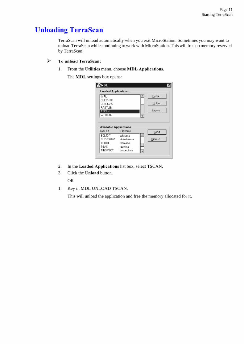
8QORDGLQJ�7HUUD6FDQTerraScan will unload automatically when you exit MicroStation. Sometimes you may want to unload TerraScan while continuing to work with MicroStation. This will free up memory reserved by TerraScan.

½ 7R�XQORDG�7HUUD6FDQ�

1. From the 8WLOLWLHV menu, choose 0'/�$SSOLFDWLRQV�

The 0'/ settings box opens:

2. In the /RDGHG�$SSOLFDWLRQV list box, select TSCAN.

3. Click the 8QORDG button.

OR

1. Key in MDL UNLOAD TSCAN.

This will unload the application and free the memory allocated for it.

7XWRULDO

Tutorial

7XWRULDO

TO BE DEFINED

7RRO�5HIHUHQFH

General tools

*HQHUDO�WRROV

*HQHUDO�WRRO�ER[The tools in the *HQHUDO tool box are used to define user settings, to define point classes, to load points, to manage section views, to place elements using laser points and to access on-line help.

7R� 8VH�

Change user settings 6HWWLQJV

Define point classes and drawing symbology 'HILQH�&ODVVHV

Load point data /RDG�3RLQWV

Rotate view to show 3D cross section 'UDZ�6HFWLRQ

Move forward or backward in section view 0RYH�6HFWLRQ

Travel along path and display sections 7UDYHO�3DWK

Adjust mouse clicks to scan point coordinates 0RXVH�3RLQW�$GMXVWPHQW

View information about TerraScan $ERXW�7HUUD6FDQ

View on-line help +HOS�RQ�7HUUD6FDQ

General tools

6HWWLQJV

6HWWLQJV tool lets you change a number of settings controling the way TerraScan works. Selecting this tool opens the TerraScan settings window.

Settings are grouped into logical categories. Selecting a category in the list causes the appropriate controls to be displayed to the right of the category list.

General tools

w.

thin r of ngle is

he

to

ation

nd

used

an a

$OLJQPHQW�UHSRUWV�FDWHJRU\

$OLJQPHQW�UHSRUWV category contains a list of alignment report formats. These will be used when outputting a tabular report where each row contains information from a specific chainage position along selected alignment. The report defines what information columns will be printed for each row.

Alignment report format definition consists of a descriptive name and a list of report columns:

Each report column will display some information computed at an increasing station position along alignment. Some data contents allow the definition of an offset from the alignment. Negative offset is left from alignment, zero offset is at alignment and positive offset is right from alignment.

The data content of a report column can be one of the following:

• Alignment station - Station or chainage value. Increases by given interval from row to ro• Alignment easting - Easting coordinate at row chainage along alignment.• Alignment northing - Northing coordinate at row chainage along alignment.• Alignment elevation - Elevation of the alignment at row chainage.• Interval elevation - Minimum or maximum elevation among laser points of given class wi

a given offset from alignment. The application will search a rectangular area. The centethe area is the alignment point at the chainage of the report row. The height of the rectatwice the offset defined in the :LWKLQ field. The width of rectangle is determined by the report interval which will be given at output time.

• Point elevation - Elevation value from laser points inside a circular area. The center of tcircular area is at the given offset from the alignment point. The elevation value can be maximum, minimum, average of all points inside circle or elevation of the point closest circle center.

• Surface elevation - Elevation from a surface model in TerraModeler. This is the only elevvalue which each computed at the exact x and y coordinate of the alignment point. ,QWHUYDO�HOHYDWLRQ and 3RLQW�HOHYDWLRQ will search points within a circular or a rectangular area aroualignment point.

• Column difference - Displays the difference between two other columns. This could be to display the height of vegetation if one column displays ground elevation and anothercolumn display maximum vegetation height.

• Alert - Displays an asterisk if the difference between two columns is bigger or smaller thgiven limit.

General tools

)LOH�H[WHQVLRQV�FDWHJRU\

)LOH�H[WHQVLRQV category defines default file extensions for various file formats. These extensions will be used only as default values when you output points from TerraScan.

)LOH�KDQGOLQJ�FDWHJRU\

)LOH�KDQGOLQJ category defines how many points will be processed at a time when loading very large files and the maximum design file size.

/HYHOLQJ�SRLQWV�FDWHJRU\

/HYHOLQJ�SRLQWV category defines the format of elevation values when drawn as text elements.

/RDGHG�SRLQWV�FDWHJRU\

/RDGHG�SRLQWV category defines how points will be highlighted when you identify a point.

2SHUDWLRQ�FDWHJRU\

2SHUDWLRQ�FDWHJRU\ defines what happens at application startup and how it is unloaded.

6HWWLQJ� (IIHFW�East North Z Default extension for plain xyz text files.Code East North Z Default extension for text files containing point class and

coordinates.TerraScan binary Default extension for binary files in TerraScan format.ArcInfo shapefile Default extension for ArcInfo shapefiles.

6HWWLQJ� (IIHFW�Points at a time Number of points to process at a time when loading a very

large file.Overlapping points Number of overlapping points which will be shared by two

consecutive parts.Size limit Maximum size for generated design file when drawing laser

points to the design file. TerraScan will stop writing when the size has been reached and will allow you to change to an empty design file before continuing. MicroStation design files can not exceed 32MB in size.

6HWWLQJ� (IIHFW�Accuracy Number of decimals to display in elevation values.Display plus If on, positive elevation values will display a plus sign.Display minus If on, negative elevation values will display a plus sign.

6HWWLQJ� (IIHFW�Hilite Color and weight for rectangle drawn around active point.

6HWWLQJ� (IIHFW�Create Applications menu If on, TerraScan will create an $SSOLFDWLRQV menu in

MicroStation’s command window at startup. This menu will contain items for opening TerraScan toolboxes.

Open Main tool box If on, the application will open its 0DLQ tool box at startup.Main tool box is closed If on, the application will be unloaded when 0DLQ tool box

is closed.

General tools

putes nt

inate

d

3RLQW�GLVSOD\�FDWHJRU\

3RLQW�GLVSOD\ category determines whether laser points will be drawn before or after design file elements.

7UDQVIRUPDWLRQV�FDWHJRU\

7UDQVIRUPDWLRQV category contains a list of coordinate transformations which are used to convert survey file coordinates into design file coordinates. Transformations can be used when loading points or outputting points.

TerraScan supports three types of coordinate transformations:

• Linear - you can assign a coefficient and a constant offset for each coordinate axis. Coma design file coordinate by multiplying the survey file coordinate with the given coefficieand by adding a given constant value.

• Equation - you can enter mathematical equations for calculating the coordinates. • Known points - you can specify the coordinates of two known points in the survey coord

system and their respective coordinates in the design file.

/LQHDU�WUDQVIRUPDWLRQ

6HWWLQJ� (IIHFW�Draw When to draw laser points:

• Before elements - laser points may be hidden by attacheraster images or design file elements.

• After elements - laser points will partially overlay and hide other types of information.

6HWWLQJ� (IIHFW�Multiply by - X Coefficient for multiplying easting.Multiply by - Y Coefficient for multiplying northing.Multiply by - Z Coefficient for multiplying elevation.Add constant - X Value to add to easting.Add constant - Y Value to add to northing.Add constant - Z Value to add to elevation.

General tools

n

(TXDWLRQ�WUDQVIRUPDWLRQ

.QRZQ�SRLQWV�WUDQVIRUPDWLRQ

:*6��FDWHJRU\

WGS84 category defines what transformations are visible from WGS84 longitudes and latitudes to planar coordinate systems. Currently only Finnish KKJ target system is available.

6HWWLQJ� (IIHFW�X Equation for calculating X coordinate. The mathematical

equation may contain:• Sx - survey file X coordinate.• Sy - survey file Y coordinate.• Sz - survey file Z coordinate.• Mathematical functions such as sin(a), cos(a), tan(a),

exp(a), log(a), log10(a), pow(a,b), sqrt(a), ceil(a), fabs(a)and floor(a) where a and b are floating point values.

Y Equation for calculating Y coordinate.Z Equation for calculating Z coordinate.

6HWWLQJ� (IIHFW�Survey X, Y, Z First known point in the survey coordinate system.X, Y, Z Second known point in the survey coordinate system.Design X, Y, Z First known point in the design file coordinate system.X, Y, Z Second known point in the design file coordinate system.

6HWWLQJ� (IIHFW�Finnish KKJ If on, conversion from WGS84 to KKJ can be selected whe

loading points.

General tools

'HILQH�&ODVVHV

'HILQH�&ODVVHV tool opens a window for managing point classes and their drawing rules.

Each laser point can be assigned a point class which defines what the laser has hit - ground, vegetation, building, wire or some other object.

Each point class is normally assigned one or more drawing rules. This will give each point or each type of target object a unique symbology. You might assign ground to be brown, vegetation green and buildings red. It is recommendable that you will assign a unique color and level for each point class.

You should create at least one point class list of your own. In the long run, you will probably want to create several class lists for different purposes. Class lists are stored as text files. Only one class list can be active at a time.

½ 7R�YLHZ�WKH�DFWLYH�FODVV�OLVW�

1. Select the 'HILQH�&ODVVHV tool.

The 3RLQW�FODVVHV window opens:

The upper list box contains a list of all point classes in the active class list. The lower list box displays all drawing rules assigned to the currently selected class. When you select another row in the class list box, the contents of the lower list will change.

½ 7R�DGG�D�QHZ�FODVV�

1. Click the $GG button.

The 3RLQW�FODVV dialog box opens:

2. Enter a unique code number and a description for the class.

The class is added to the active class list. You will now probably want to assign drawing rules to the new class.

6HWWLQJ� (IIHFW�Code Code number for the class. Each class should have unique

number.Description Descriptive name for the class.

General tools

Point class

evious

lasses

½ *HQHUDO�SURFHGXUH�IRU�DGGLQJ�GUDZLQJ�UXOHV�WR�D�FODVV�

1. Select the desired class in the upper list box.

2. Click the $GG button on the side of the lower list box.

The 'UDZLQJ�UXOH dialog box opens:

3. Choose the drawing rule type and fill in settings values. In most cases you will want to draw laser points using =HUR�OHQJWK�OLQH drawing rule type.

4. Click OK.

The new drawing rule is added to the lower list box which displays all rules assigned for the selected class.

&ODVV�OLVW�ILOHV

Class lists are stored as text files which have defualt extension “*.ptc”. The File menu in theclasses window has commands for opening existing class list files and for saving the activelist into a file.

When you start TerraScan, it automatically loads the class list which was used during the prwork session.

You can use a text editor to edit class list files. This may prove useful if you need to copy cand drawing rules from one class list to another.

General tools

/RDG�3RLQWV

/RDG�3RLQWV tool reads points from one or several files for processing. You will always use this tool before you start working on laser points.

This tool will recognize the file format of the selected files automatically if those are supported by the application.

½ /RDGLQJ�SRLQWV�IRU�SURFHVVLQJ�

1. Select the /RDG�SRLQWV tool.

This opens a dialog which allows you to select one or several files to process.

2. Add the desired file(s) to the list of files to process and click Done.

The /RDG�'DWD�3RLQWV dialog opens. The coordinate axes show the coordinate values of the first point found in the survey file. This will help you to select an optional coordinate transformation that will convert the points into the design file coordinate system.

3. Enter settings values and click OK.

TerraScan reads all selected files into memory and opens the /RDGHG�SRLQWV window which lets you classify and manipulate the points.

See chapter :RUNLQJ�ZLWK�ORDGHG�SRLQWV on page 30 for more information on working with laser points.

6HWWLQJ� (IIHFW�Transform Coordinate transformation for converting input file

coordinates into design file coordinates.Default Default point class assigned to all points when incoming file

does not contain class information.Load partial file This setting is selectable only when reading in a single file.

If on, you can select which small part of a large file to process.

General tools

'UDZ�6HFWLRQ

'UDZ�6HFWLRQ tool creates a 3D section view from a position defined by two points.

Section view is simply a rotated MicroStation view which will display all visible design file elements and laser points inside the given slice of space. This makes it ideal for viewing laser points and for placing vector elements. If you use a section view to place elements, they will be drawn to a true 3D position.

½ 7R�GUDZ�D�VHFWLRQ�YLHZ�

1. Select the 'UDZ�6HFWLRQ tool.

2. Enter start or left point for section line.

3. Enter end or right point for section line.

4. Define section view depth by entering a data click or by keying in a value in the 'HSWK field.

5. Identify view to be used as the section view.

This view will be rotated to show a cross section. The application will automatically compute the required elevation range so that all laser points inside the given section rectangle will be visible.

6HWWLQJ� (IIHFW�Depth Display depth on both sides of section line.

General tools

0RYH�6HFWLRQ

0RYH�6HFWLRQ tool lets you traverse cross section by stepping a sectional view forward or backward.

The step size can be set to full or half of the view section depth.

½ 7R�PRYH�VHFWLRQDO�YLHZ�IRUZDUG�RU�EDFNZDUG�

1. Start 0RYH�6HFWLRQ tool.

2. Move the mouse to a view window which you want to move forward or backward.

When the mouse is in a sectional view, the system will display the content rectangle of that view in all top views (and rotated top like views).

3. Click left mouse button (data click) to move the view forward.

or

3. Click right mouse button (reset click) to move the view backward.

This will move the section view and update the dynamic content rectangle in all top like views.

6HWWLQJ� (IIHFW�Move by Step size:

• Half of view depth - Half of the content rectangle will be visible in the next section when moved.

• Full view depth - Content rectangles thouch each other but do now overlap.

General tools

laser

lect

.

f

7UDYHO�3DWK

7UDYHO�SDWK tool lets you view a flythru along an alignment. You can define what kind of views you want to see while traveling along the alignment. Supported view types include top, cross section, longitudinal section and isometric views.

This tool provides an excellent way for traversing along the survey path and checking the data visually.

The alignment element can be any linear MicroStation design file element. In most cases you would create that element manually. Alternatively, you can use TerraScan’s 'UDZ�SDWK menu command which will draw an approximate flight path as deduced from the order of importedpoints.

½ 7R�FUHDWH�D�IO\WKUX�DORQJ�DQ�DOLJQPHQW�

1. Select the alignment element.

2. Select the 7UDYHO�3DWK tool.

This opens the 7UDYHO�3DWK dialog:

3. Enter desired cross section step and width.

4. Click OK.

This opens the 7UDYHO�3DWK�9LHZV dialog:

5. Set on each view type which you want see while traveling along the alignment and sethe view windows in which you want those drawn.

6. Click OK.

The application constructs internal tables for the flythru and then opens the 7UDYHO�3OD\HU dialog.

6HWWLQJ� (IIHFW�Step Step along alignment between consecutive cross sections

Same as depth of cross sections.Width Width of cross sections. The cross section will display a

rectangular area which extends half width to the left and halwidth to the right from alignment.

General tools

7UDYHO�3OD\HU supports the following tools for traveling along the alignment:

0HQX� 7RRO�QDPH� (IIHFW�

Move 8VLQJ�PRXVHUpdate the cross section view dynamically as you move the mouse along the alignment. If you click the mouse, the tool will update all travel views.

Move 7R�VWDUW Rewind to the start of the alignment.Move 7R�HQG Move to the end of the alignment.

3OD\�EDFNZDUG Start traversing backward along the alignment.

6WHS�EDFNZDUG Step one cross section backward and stops.

6WRS Stop traversing.

6WHS�IRUZDUG Step one cross section forward and stops.

3OD\�IRUZDUG Start traversing forward along the alignment.

General tools

een

0RXVH�3RLQW�$GMXVWPHQW

0RXVH�3RLQW�$GMXVWPHQW tool lets you place elements to the location or the elevation of laser points. You can use this tool with any MicroStation element placement tool. 0RXVH�3RLQW�$GMXVWPHQW simply adjusts the coordinates of the mouse clicks.

You can choose if the elevation of the mouse click and if the xy location of the mouse click is to be adjusted. If you want to digitise a small wire, you would want to both the xy and the elevation of the mouse clicks to come from the laser points. On the other hand, if you want to place a linear feature on the ground, you would probably want to adjust only the elevation of the mouse clicks.

½ 7R�SODFH�HOHPHQWV�DFFRUGLQJ�WR�ODVHU�SRLQWV�

1. Select the 0RXVH�3RLQW�$GMXVWPHQW tool.

This opens the 0RXVH�3RLQW�$GMXVWPHQW window:

2. Select desired setting values.

3. Start the drawing primitive you want to use and place the element(s).

As long as 0RXVH�3RLQW�$GMXVWPHQW window is open, all the active locks will be applied to all mouse clicks.

? Be sure to always close the 0RXVH�3RLQW�$GMXVWPHQW window after using it. As it will alter all mouse clicks, it may interfere with your normal work if you forget it is active.

You can not use MicroStation’s tentative to snap on to laser points if the points have not bdrawn to the design file as permanent elements.

6HWWLQJ� (IIHFW�Adjust elevation If on, elevation of mouse clicks will be adjusted.Dz Constant to add to laser point elevation.Adjust xy If on, xy location of mouse clicks will be adjusted.Class Class of points to adjust to.Point Point to adjust to:

• Closest – point closest to mouse click.• Highest – highest point within search circle.• Average – average xyz of all points within search circle.• Lowest – lowest point within search circle.

Within Radius of search area circle around mouse location.

General tools

$ERXW�7HUUD6FDQ

$ERXW�7HUUD6FDQ tool opens a window which shows information on TerraScan and on user license.

+HOS�RQ�7HUUD6FDQ

+HOS�RQ�7HUUD6FDQ tool launches Acrobat Reader for accessing on-line help.

The on-line help is identical in structure to the printed documentation. The on-line version has hypertext links built in, so you can jump between topics by clicking on the underlined topic names.

? Floppy based installation does not include on-line documentation. You can access on-line help only if you have installed from CD. Accessing on-line help also requires that you have Acrobat Reader installed on your computer.

Working with loaded points

or the

you uld

laser .

will round

:RUNLQJ�ZLWK�ORDGHG�SRLQWV

When you load data using /RDG�3RLQWV tool, the application reads the laser points into RAM memory and opens the /RDGHG�SRLQWV window. As long as you keep this window open, the points will remain in memory and will be displayed in all open views with appropriate levels on. You can use various tools for viewing, classifying, manipulating or outputting the loaded points.

Typical workflow includes the following steps:

1. Read laser points from raw files generated by system manufacturer’s applications.

2. Delete points which go outside the geographical area of interest.

3. Search and delete error points (points high up in the air or below the ground).

4. Classify points into point classes such as ground, vegetation, building or wire.

5. Save modified points into a separate file which you can load if you start another worksession later on.

6. Create vectors into the design file based on the points. This might involve automatic detection of some features such as wires or manual digitization using the coordinateselevations of laser points.

Throughout the work session you will be using various viewing tools to see the data in 3D.

0HPRU\�XVDJH

The amount of RAM memory in your computer will probably set the limit on how large jobs can process at one time. Each loaded laser point will take up 24 bytes of memory. You shonormally plan your work so that you will have enough physical memory to accommodate thepoints you process. Virtual memory (hard disk) usage will drastically slow TerraScan down

Basic total memory usage consists roughly of:

• 30 MB for Windows NT• 12 MB for MicroStation and design file• 24 MB for every million laser points loaded

You should also note that some classification routines will allocate substantial amounts of memory temporarily. The most demanding routine is probably ground classification which take up an additional 4 bytes for every point and 80 bytes for each point that ends up in the gclass.

Depending on the type of tools you need to use, you can process upto:

• 2-3 million points with 128 MB RAM• 5-8 million points with 256 MB RAM• 12-18 million points with 512 MB RAM


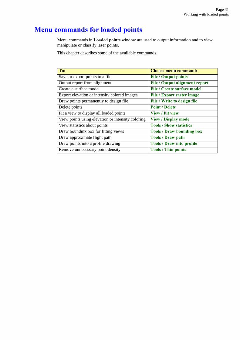
0HQX�FRPPDQGV�IRU�ORDGHG�SRLQWVMenu commands in /RDGHG�SRLQWV window are used to output information and to view, manipulate or classify laser points.

This chapter describes some of the available commands.

7R� &KRRVH�PHQX�FRPPDQG�Save or export points to a file )LOH��2XWSXW�SRLQWVOutput report from alignment )LOH��2XWSXW�DOLJQPHQW�UHSRUWCreate a surface model )LOH��&UHDWH�VXUIDFH�PRGHOExport elevation or intensity colored images )LOH��([SRUW�UDVWHU�LPDJHDraw points permanently to design file )LOH��:ULWH�WR�GHVLJQ�ILOHDelete points 3RLQW��'HOHWHFit a view to display all loaded points 9LHZ��)LW�YLHZView points using elevation or intensity coloring 9LHZ��'LVSOD\�PRGHView statistics about points 7RROV��6KRZ�VWDWLVWLFVDraw boundinx box for fitting views 7RROV��'UDZ�ERXQGLQJ�ER[Draw approximate flight path 7RROV��'UDZ�SDWKDraw points into a profile drawing 7RROV��'UDZ�LQWR�SURILOHRemove unnecessary point density 7RROV��7KLQ�SRLQWV


)LOH��2XWSXW�SRLQWV

2XWSXW�SRLQWV menu command writes laser points into a text file or a binary file. You can use this to save your work or to export points for another system.

The output file format can be any of the following:

• East North Z – plain xyz text file.• Code East North Z – text file with class, x, y and z for each point.• TerraScan binary – compact and fast file format which includes all laser point information. Best

format for saving the points between work sessions.• ArcInfo shapefile – format used by ArcInfo products.

½ 7R�ZULWH�SRLQWV�LQWR�D�ILOH�

1. Choose 2XWSXW�SRLQWV command from )LOH menu.

This opens the 2XWSXW�SRLQWV dialog:

2. Select point classes which you want to output.

3. Select file format in )RUPDW field.

4. Click OK.

A standard dialog box for choosing an output file name opens.

5. Enter a name for the output file.

A file with the given name is created and points in selected classes are written to it.


)LOH��2XWSXW�DOLJQPHQW�UHSRUW

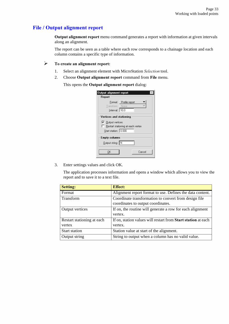
2XWSXW�DOLJQPHQW�UHSRUW�menu command generates a report with information at given intervals along an alignment.

The report can be seen as a table where each row corresponds to a chainage location and each column contains a specific type of information.

½ 7R�FUHDWH�DQ�DOLJQPHQW�UHSRUW�

1. Select an alignment element with MicroStation 6HOHFWLRQ tool.

2. Choose 2XWSXW�DOLJQPHQW�UHSRUW command from )LOH menu.

This opens the 2XWSXW�DOLJQPHQW�UHSRUW dialog:


The application processes information and opens a window which allows you to view the report and to save it to a text file.

6HWWLQJ� (IIHFW�Format Alignment report format to use. Defines the data content.Transform Coordinate transformation to convert from design file

coordinates to output coordinates.Output vertices If on, the routine will generate a row for each alignment

vertex.Restart stationing at each vertex

If on, station values will restart from 6WDUW�VWDWLRQ at each vertex.

Start station Station value at start of the alignment.Output string String to output when a column has no valid value.


)LOH��&UHDWH�VXUIDFH�PRGHO

&UHDWH�VXUIDFH�PRGHO menu command passes points in selected class to TerraModeler which creates a triangulated surface model. You would normally use this to create a ground surface model after having classified and possibly thinned the points.

This menu command requires a separate user license for TerraModeler.

½ 7R�FUHDWH�D�WULDQJXODWHG�VXUIDFH�PRGHO�

1. Choose &UHDWH�VXUIDFH�PRGHO command from )LOH menu.

This loads TerraModeler if not loaded already and opens the &UHDWH�VXUIDFH�PRGHO dialog:

2. Select point class to triangulate and click OK.

TerraModeler creates a triangulated surface model from the points.

? After this operation both TerraScan and TerraModeler will end up keeping copies of the points in memory. If you want to reduce the memory requirement, you can follow the following steps:

1. Load, classify and thin the laser points using TerraScan.

2. Write points to an xyz text file using )LOH��2XWSXW�SRLQWV menu command.

3. Unload TerraScan.

4. Load TerraModeler.

5. Import points from text file.


le.g

)LOH��([SRUW�UDVWHU�LPDJH

([SRUW�UDVWHU�LPDJH menu command generates a raster image colored by elevation or intensity of laser points.

The raster image will be created in Windows bitmap (BMP) format. The color of each pixel will be determined using laser points whose coordinate values fall inside the pixel rectangle. The coloring principle can be chosen as:

• Elevation – Laser point elevation.• Elevation difference – Elevation difference between laser points of two different classes.• Intensity hits – Intensity of laser points with center point inside the pixel.• Intensity footprint – Intensity of laser points with footprint overlapping the pixel.

½ 7R�FUHDWH�D�FRORUHG�UDVWHU�LPDJH�

1. Choose ([SRUW�UDVWHU�LPDJH menu command.

This opens the ([SRUW�5DVWHU�,PDJH dialog:


A standard dialog box for choosing an output file name opens.

3. Enter a name for the output file.

This creates a raster image with the given name.

6HWWLQJ� (IIHFW�Color by Coloring principle.Class Point class to use.Value Value determination within each pixel:

• Lowest – Smallest value of the points.• Average – Average value of the points.• Highest – Highest value of the points.

Colors Color depth of raster image:• 24 Bit Color — true color image.• 256 Colors — 256 colors.• Grey scale — 8 bit grey scale.

Pixel size Size of each pixel.Fill gaps If on, fill small gaps in places where there are no laser hits

inside a pixel.Attach as reference If on, attach the image as raster reference to the design fiDraw placement rectangle If on, draw the image position as a shape. Helps in attachin

the image to the correct location later on.


Scheme Type of coloring scheme:• Cold to hot – varies from blue in low elevation to red in

high elevation.• Hot to cold – varies from red in high elevation to blue in

low elevation.• Selected colors – you can define the coloring scheme.

Degree Determines how the color changes in &ROG�WR�KRW and +RW�WR�FROG schemes are computed.

6HWWLQJ� (IIHFW�


)LOH��:ULWH�WR�GHVLJQ�ILOH

:ULWH�WR�GHVLJQ�ILOH menu command draws laser points permanently into the design file using all of the drawing rules assigned to point classes.

MicroStation design files are limited to a maximum size of 32MB. This means that you can draw about half a million laser points into one design file if using =HUR�OHQJWK�OLQH drawing rules.

If the design file grows larger than user specified 6L]H�OLPLW (File handling category in user settings), this routine will end the writing process, remove processed points from the table and tell you what has happened. You can then switch to an empty design file and restart the writing process.

3RLQW��'HOHWH

'HOHWH submenu contains commands for deleting points:

• Selected points – Deletes the point(s) selected in the list.• By point class – Deletes all points in a class you choose.• Inside fence – All points inside the fence and on visible levels.• Outside fence – All points outside the fence and on visible levels.• Using centerline – All points which are too far away from the selected centerline element. You

can choose the offset distance limit.

9LHZ��)LW�YLHZ

)LW�YLHZ menu command sets a view to top rotation and fits it to display an area covering all of the loaded points.

½ 7R�ILW�D�YLHZ�WR�GLVSOD\�DOO�SRLQWV�

1. Choose )LW�YLHZ command from 9LHZ menu.

2. Select a view by clicking inside the view.

Application sets the view into top orientation, fits to loaded points and redraws. You can continue to step 2.

See 7RROV��'UDZ�ERXQGLQJ�ER[ on page 39 for information on how to fit a rotated view to display all loaded points.


9LHZ��'LVSOD\�PRGH

'LVSOD\�PRGH menu command lets you control how laser points are colored in view windows. Normally laser points are drawn using colors assigned to point class drawing rules. 'LVSOD\�PRGH command lets you turn on elevation or intensity based coloring.

½ 7R�GHILQH�WKH�GLVSOD\�PRGH�

1. Choose Display mode command from View menu.

This opens the Display mode dialog:

2. Check views in (OHYDWLRQ�FRORULQJ group if you want to see points colored by elevation and click Colors to define what colors to use.

3. Check views in ,QWHQVLW\�FRORULQJ group if you want to see points colored by intensity and click Colors to define what colors to use.

4. Click OK.

6HWWLQJ� (IIHFW�Use depth in 3D views If on, eah pixel in a rotated view will be colored using the

pixel closest to viewer. Improves the visual image of dense point clouds in cities.


only

ints.

r duces

ts by

nts.

7RROV��6KRZ�VWDWLVWLFV

6KRZ�VWDWLVWLFV menu command display basic statistics about laser points. You can choose whether to view statistics of all the points or points in a specific class only.

7RROV��'UDZ�ERXQGLQJ�ER[

'UDZ�ERXQGLQJ�ER[ menu command draws a bounding box around all of the loaded points. This is useful if you want to fit rotated views to display all laser points. Because laser points are kept in TerraScan’s memory, MicroStation is not aware of those and will use design file elementswhen fitting a view.

This command draws a graphical group of twelve line elements which enclose all laser poYou can then use MicroStation )LW�9LHZ tool to fit rotated views.

7RROV��'UDZ�SDWK

'UDZ�SDWK menu command draws an approximate flight path into the design file as a lineaelement. This will work only if the laser points are in original scan order as the command dethe flight path from laser points only.

The created linear element can be used as an alignment for drawing profiles, deleting poincenterline or outputting alignment reports.

½ 7R�GUDZ�DQ�DSSUR[LPDWH�IOLJKW�SDWK�

1. Choose 'UDZ�SDWK command from 7RROV menu.

This opens the 'UDZ�3DWK dialog:

2. Enter maximum gap and click OK.

This computes the approximate flight path and draws it as one or several linear eleme

6HWWLQJ� (IIHFW�Maximum gap Starts a new path element whenever the distance between

two consecutive laser points exceeds this value.


7RROV��'UDZ�LQWR�SURILOH

'UDZ�LQWR�SURILOH menu command draws laser points into a profile or a cross section as permanent elements. This command will draw all points in a given class which are within the given offset limit from the profile alignment.

You should create the profile or the cross sections using TerraModeler.

½ 7R�GUDZ�ODVHU�SRLQWV�LQWR�D�SURILOH�

1. Choose 'UDZ�LQWR�SURILOH command from 7RROV menu.

This opens the 'UDZ�LQWR�SURILOH dialog:


3. Identify the profile cell element.

This draws the points into the profile.


7RROV��7KLQ�SRLQWV

7KLQ�SRLQWV menu command removes unnecessary point density by deleting some of the points which are close to each other. You would often use this to thin ground points before creating a triangulated surface model.

This routine will only remove points which have another point within a given horizontal distance limit and within a given elevation difference limit.

½ 7R�WKLQ�SRLQWV�

1. Select 7KLQ�SRLQWV command from 7RROV menu.

This opens the 7KLQ�SRLQWV dialog:


This deletes some of the points in the givel class.

6HWWLQJ� (IIHFW�From class Class from which to delete unnecessary points.Keep Which point to keep in a group of close points:

• Highest point – Point with highest elevation.• Lowest point – Point with lowest elevation.• Central point – Point in the middle of the group.• Create average – Substitute group by creating an average.

Distance Horizontal distance limit between two points.Dz Elevation difference limit between two points.

Powerline processing

3RZHUOLQH�SURFHVVLQJ

TerraScan has a number of tools which are dedicated to powerline processing. These include both classification, vectorization and reporting tools.

The general strategy for processing powerline data can be outlined as:

1. Classify ground points using *URXQG routine.

2. Classify high points which may be hits on wires or towers using %\�PLQLPXP�HOHYDWLRQ or %\�KHLJKW�IURP�JURXQG routines.

3. Classify rest of the points (possibly all as vegetation).

4. Manually place a tower string to run from tower to tower using 3ODFH�7RZHU�6WULQJ tool.

5. Detect wires automatically using 'HWHFW�ZLUHV menu command.

6. Manually place wires using 3ODFH�&DWHQDU\�6WULQJ tool in places where automatic detection does not work.

7. Validate and adjust catenary curves using &KHFN�&DWHQDU\�$WWDFKPHQWV tool.

8. Create required drawings with the help of labeling tools.

9. Output required reports.


3RZHUOLQH�WRRO�ER[The tools in the 3RZHUOLQH tool box are used to place powerline centerline, to manually place catenaries, to validate catenary attachment points and to label distances from catenaries to ground or vegetation.

7R� 8VH�

Place a line string from tower to tower 3ODFH�7RZHU�6WULQJ

Digitize a catenary line string 3ODFH�&DWHQDU\�6WULQJ

Check catenary attachment points at towers &KHFN�&DWHQDU\�$WWDFKPHQWV

Label height from ground to catenary /DEHO�&DWHQDU\�+HLJKW

Label minimum distance to catenary /DEHO�&DWHQDU\�0LQLPXP�'LVWDQFH


3ODFH�7RZHU�6WULQJ

3ODFH�7RZHU�6WULQJ tool is used to manually place an approximate centerline from tower to tower. This tower string will be used in later processing steps when detecting wires, validating catenary attachment points or producing reports along the powerline.

Tower string is a line string or a complex chain which runs along the powerline with a vertex at each tower.

3ODFH�7RZHU�6WULQJ tool integrates line string placement and view panning in one tool.

½ 7R�SUHSDUH�IRU�WRZHU�VWULQJ�SODFHPHQW�

1. Classify all higher points into a unique point class using %\�PLQLPXP�HOHYDWLRQ or %\�KHLJKW�IURP�JURXQG routines. This is to separate all points which are high from the ground and which may be hits on towers or wires. The classified high points will also include hits on other high objects such as trees and buildings.

2. Choose a view which you will use as 7RS�YLHZ for placement.

3. Switch the level of high points on and the levels of all other point classes off in that view.

4. Zoom in close to a tower so that you can clearly see where the tower is located. Normally this means that you will see only one tower and some wire hits which indicate the direction where the powerline continues.

5. Set active color and active level so that the tower string will be placed on a level with no other elements.

½ 7R�SODFH�D�WRZHU�VWULQJ�

1. Select the 3ODFH�7RZHU�6WULQJ tool.

2. Make sure 7RS�YLHZ option button is set as the view you have chosen.

3. Enter a point to at the approximate center of the first tower.

The first tower location has been given. The application will now draw a dynamic rectangle in the 7RS�YLHZ whenever you move the mouse inside view windows. If you enter a point outside the rectangle, the application will pan the view in the direction of the mouse click. Entering a point inside the rectangle adds a new vertex to the tower string.

4. Enter a mouse click outside the dynamic rectangle to move the view in the direction of the powerline.

5. Repeat step 4 until you see the next tower inside the dynamic rectangle.

6. Enter a point to at the approximate center of the next tower.

7. Continue to step 4 or enter reset to end placement.

6HWWLQJ� (IIHFW�Top view View in which the dynamic rectangle will be drawn and

which can be panned by clicking outside the rectangle.Profile view An optional view which will display a profile along the

direction of tower string you are creating. You will need this if you can not see the locations of towers from a top like view. The profile view will show the curvature of catenary wires to help locate towers.


? As an end result of tower string placement, you should get a single line string or complex chain type element. It may happen that you can not place the entire tower string as one operation. In this case you should continue by placing another tower string which runs in the same direction and starts at the exact end point of the previous one. When you have placed a number of shorter tower strings, you can join those using MicroStation’s &UHDWH�&RPSOH[�&KDLQ tool.


3ODFH�&DWHQDU\�6WULQJ

3ODFH�&DWHQDU\�6WULQJ tool lets you manually place a single catenary curve between two towers. You should use this tool in places where automatic detection of wires does not work. This happens normally when you have a very small number of hits on the wire.

You define the mathematical shape of the catenary curve with three mouse clicks. In most cases you would use 6QDS�WR lock to use the xyz coordinates of closest laser hits.

You can enter optional mouse clicks to define the start location and the end location of the catenary curve. These affect the length of the catenary only. You would normally use this feature to extend the catenary curve to cover the whole distance from tower to tower. You can snap the start location on to an end point of an incoming wire or on to a tower string vertex. Similarly, you can snap the end location on to a start point of an outgoing wire or on to a tower string vertex.

In order to improve the accuracy of the catenary curve, you can apply least squares fitting. The manually entered three curvature points define the initial shape of the catenary. The application will then search all points which are within a tolerance distance from the manually entered curve and use those points in the fitting phase.

½ 7R�SUHSDUH�IRU�FDWHQDU\�SODFHPHQW�

1. Use 'UDZ�6HFWLRQ tool to create a longitudinal section along the wire from tower to tower.

2. Set active color and active level to place the catenary on a dedicated level.

½ 7R�SODFH�D�FDWHQDU\�FXUYH�PDQXDOO\�

1. Select the 3ODFH�&DWHQDU\�6WULQJ tool.

2. (Optional) Enter a start location point at the start tower.

3. Enter the first curvature point.

4. Enter the second curvature point.

5. Enter the third curvature point.

6. (Optional) Enter an end location point at the end tower.

The application draws the catenary curve defined by the given points.

7. Accept the catenary curve.

The catenary curve is added to the design file. You can continue to step 2.

6HWWLQJ� (IIHFW�Start location separately If on, first point defines the start location of the catenary.Snap to If on, adjust the three curvature points to the coordinates of

closest laser points of a given class. This lock is normally on.Fit using If on, the catenary curve will be fitted to laser points. Classify to If on, classify points to a given class. Affects points within a

given tolerance from the final curve.End location separately If on, last point defines the end location of the catenary.


&KHFN�&DWHQDU\�$WWDFKPHQWV

&KHFN�&DWHQDU\�$WWDFKPHQWV tool validates and adjusts catenary curves. It checks the gaps between catenary curves at tower locations. Because each catenary curve has been computed using laser points from one tower to tower span only, the incoming curve and the outgoing curve do not meet exactly. The magnitude of the gap gives some indication of how accurately the catenaries have been detected or placed.

½ 7R�YDOLGDWH�FDWHQDU\�DWWDFKPHQW�SRLQWV�

1. Select tower string element using MicroStation 6HOHFWLRQ tool.

2. Select the &KHFN�&DWHQDU\�$WWDFKPHQWV tool.

This opens the &KHFN�&DWHQDU\�$WWDFKPHQWV dialog:

PICTURE


The application searches for catenaries from given levels, finds meeting pairs and computes gaps between the incoming and the outgoing catenaries.

TO BE DEFINED

6HWWLQJ� (IIHFW�

From levelsList of levels from which to search catenaries. For example:• 50 – level 50.• 15,21-24 – levels 15,21,22,23 and 24.

FirstNumber of the tower at first vertex in the selected tower string.

XyXy gap flagging limit. Gaps exceeding this value will be drawn in red color in the list.

Z Z gap flagging limit.Shift Tower shift flagging limit.


/DEHO�&DWHQDU\�+HLJKW

/DEHO�&DWHQDU\�+HLJKW tool labels the minimum height from a catenary curve to a point class such as ground.

It searches all the points which are within a given offset limit from the line of the catenary. The minimum height difference from a point to the catenary is labeled with a text element and a vertical line using active symbology.

½ 7R�ODEHO�KHLJKW�IURP�FDWHQDU\�WR�JURXQG�

1. Select the /DEHO�&DWHQDU\�+HLJKW tool.

2. Select ground class in the )URP�FODVV option button.

3. Identify a catenary string element.

4. Accept the catenary string to labeled.

Minimum height difference is labeled. You can continue to step 3.

6HWWLQJ� (IIHFW�From class Class to compare catenary curve with. Normally set to

ground class.Within Maximum search offset on both sides of catenary line.


/DEHO�&DWHQDU\�0LQLPXP�'LVWDQFH

/DEHO�&DWHQDU\�0LQLPXP�'LVWDQFH tool labels the minimum distance from a catenary curve to points in a selected class such as vegetation.

It searches all the points which are within a given offset limit from the line of the catenary. The smallest three dimensional distance from a point to the catenary is labeled with a text element and a line using active symbology.

½ 7R�ODEHO�PLQLPXP�GLVWDQFH�WR�YHJHWDWLRQ�

1. Select the /DEHO�&DWHQDU\�0LQLPXP�'LVWDQFH tool.

2. Select ground class in the )URP�FODVV option button.

3. Identify a catenary string element.

4. Accept the catenary string to labeled.

Minimum height difference is labeled. You can continue to step 3.

6HWWLQJ� (IIHFW�From class Class to compare catenary curve with. Normally set to

vegetation class.Within Maximum search offset on both sides of catenary line.

Railroad processing

5DLOURDG�SURFHVVLQJ

TerraScan has a few tools which are dedicated to railroad processing. These include both classification and vectorization tools.

The general strategy for processing railroad data can be outlined as:

1. Classify points which may be hits on the rails. This step serves the purpose of getting a visual image of where the railroad runs. If intensity information is available, use %\�LQWHQVLW\ routine as classifying high intensity returns often provides the best visual image. If intensity information is not available, use 5DLOURDG routine to classify points which match rail elevation pattern.

2. Manually place railroad centerlines using 3ODFH�5DLOURDG�6WULQJ tool.

3. Restore rail hits classified in step 1 back to the original class.

4. Classify rail hits using 5DLOURDG routine with railroad centerlines as alignments. This will classify points with correct elevation pattern and within the right offset (half rail width) from manually placed centerline.

5. Fit centerlines to classified points using )LW�5DLOURDG�6WULQJ tool.

6. Classify rest of the points into ground, vegetation and other appropriate classes.

7. Manually digitize relevant objects along the railroad track with the help of images and laser points.

Railroad processing

5DLOURDG�WRRO�ER[The tools in the 5DLOURDG tool box are used to place railroad centerlines and to fit centerlines to classified points.

7R� 8VH�

Place approximate railroad centerline 3ODFH�5DLOURDG�6WULQJ

Fit railroad centerline to laser points )LW�5DLOURDG�6WULQJ

Railroad processing

3ODFH�5DLOURDG�6WULQJ

3ODFH�5DLOURDG�6WULQJ tool is used to manually place an approximate centerline between two rails. This manually placed centerline can be used later on to classify rail hits and to fit the centerline to classified hits.

It is a good idea to create a custom line style definition for the rails. The custom line style should consist of two lines which are railroad width apart. This gives you the benefit of viewing the railroad string as a centerline or as a pair of rails simply by swithing line styles on or off in a view.

3ODFH�5DLOURDG�6WULQJ tool integrates line string placement and view panning in one tool.

½ 7R�SUHSDUH�IRU�UDLOURDG�VWULQJ�SODFHPHQW�

1. Classify potential rail hits into a unique point class using %\�LQWHQVLW\ or 5DLOURDG routines. This initial classification will probably include a number of points which are not hits on rails. However, the only goal at this stage is to get a visual image of where the railroad runs.

2. Switch the level of rail points on and the levels of all other point classes off in a view.

3. Set active color and select the railroad custom style as the active line style.

4. Set active level so that the railroad string will be placed on a level with no other elements.

½ 7R�SODFH�D�UDLOURDG�VWULQJ�

1. Select the 3ODFH�5DLOURDG�6WULQJ tool.

2. Enter a point to at the approximate centerline between two rails.

The first point has been given. The application will now draw a dynamic rectangle whenever you move the mouse inside view windows. If you enter a point outside the rectangle, the application will pan the view in the direction of the mouse click. Entering a point inside the rectangle adds a new vertex to the tower string.

3. (Optional) Enter a mouse click outside the dynamic rectangle to move the view in the direction of the powerline.

4. Enter a point to at the approximate center of the next tower.

5. Continue to step 3 or enter reset to end placement.

Railroad processing

)LW�5DLOURDG�6WULQJ

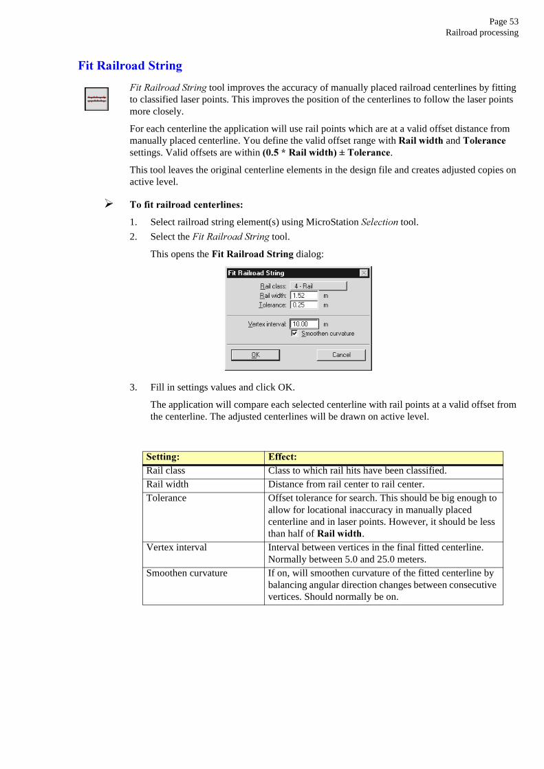
)LW�5DLOURDG�6WULQJ tool improves the accuracy of manually placed railroad centerlines by fitting to classified laser points. This improves the position of the centerlines to follow the laser points more closely.

For each centerline the application will use rail points which are at a valid offset distance from manually placed centerline. You define the valid offset range with 5DLO�ZLGWK and 7ROHUDQFH settings. Valid offsets are within �� 5DLO�ZLGWK��7ROHUDQFH.

This tool leaves the original centerline elements in the design file and creates adjusted copies on active level.

½ 7R�ILW�UDLOURDG�FHQWHUOLQHV�

1. Select railroad string element(s) using MicroStation 6HOHFWLRQ tool.

2. Select the )LW�5DLOURDG�6WULQJ tool.

This opens the )LW�5DLOURDG�6WULQJ dialog:

3. Fill in settings values and click OK.

The application will compare each selected centerline with rail points at a valid offset from the centerline. The adjusted centerlines will be drawn on active level.

6HWWLQJ� (IIHFW�Rail class Class to which rail hits have been classified.Rail width Distance from rail center to rail center.Tolerance Offset tolerance for search. This should be big enough to

allow for locational inaccuracy in manually placed centerline and in laser points. However, it should be less than half of 5DLO�ZLGWK.

Vertex interval Interval between vertices in the final fitted centerline. Normally between 5.0 and 25.0 meters.

Smoothen curvature If on, will smoothen curvature of the fitted centerline by balancing angular direction changes between consecutive vertices. Should normally be on.

&ODVVLILFDWLRQ�5HIHUHQFH

Classification routines

&ODVVLILFDWLRQ�URXWLQHV

The menu in /RDGHG�SRLQWV window offers a number of classification tools. This chapter describes the basic logic used in various classification routines.

%\�FODVV

%\�FODVV routine simple changes all points in a given class to another class.

á You can often use this to undo a classification.

/RZ�SRLQWV

/RZ�SRLQWV routine classifies points which are lower than other points in the vicinity. It is often used to search for possible error points which are clearly below the ground.

This routine will basically compare the elevation of each point (=center) with every other point within a given xy distance. If the center point is clearly lower than any other point, it will be classified.

Sometimes you may have a higher density of error points. If there are several error points close to each other, those will not be detected if searching for single low points. However, this routine can also search for groups of low points where the whole group is lower than other points in the vicinity.

6HWWLQJ� (IIHFW�From class Source class from which to classify points.To class Target class to put points into.Search Whether to search for groups or single points.Max count Maximum size of a group of low points.More than Minimum height difference. This is normally 0.3 - 1.0 m.Within Xy search range. Each point is compared with every other

point less than :LWKLQ distance away. Normally 2.0 - 8.0 m.


*URXQG

*URXQG routine classifies ground points by iteratively building a triangulated surface model.

The routine starts by selecting some local low points as sure hits on the ground. You control initial point selection with the 0D[�EXLOGLQJ�VL]H parameter. If maximum building size is 60.0 m, the application can assume that any 60 by 60 m area will have at least one hit on the ground (provided there are points around different parts of the area) and that the lowest point is a ground hit.

The routine builds an initial model from selected low points. Triangles in this initial model are mostly below the ground with only the vertices touching ground. The routine then starts molding the model upwards by iteratively adding new laser points to it. Each added point makes the model follow ground surface more closely.

Iteration parameters determine how close a point must be to a triangle plane so that the point can be accepted to the model. ,WHUDWLRQ�DQJOH is the maximum angle between point, its projection on triangle plane and closest triangle vertex. ,WHUDWLRQ�GLVWDQFH parameter makes sure that the iteration does not make big jumps upwards when triangles are large. This helps to keep low buildings out of the model.

The smaller the ,WHUDWLRQ�DQJOH, the less eager the routine is to follow changes in the point cloud (small undulations in terrain or hits on low vegetation). Use a small angle (close to 8.0) in flat terrain and a bigger angle (close to 20.0) in hilly terrain.


$GGLQJ�WR�SRLQWV�WR�JURXQG

It is generally advisable to run *URXQG classification using an ,WHUDWLRQ�DQJOH which is too small rather than too big. It is easier to add points to ground than to remove points from it.

Ground terrain may have some small formations which you want to reprocess locally. One way to do this is using $GG�SRLQW�WR�JURXQG menu command. It lets you identify an unclassified point which belongs to ground, adds that to ground model and reprocesses the surroundings.

6HWWLQJ� (IIHFW�From class Source class from which to classify points.To class Target class to put points into.Select Selection of initial ground points. Use &XUUHQW�JURXQG�

SRLQWV when you want to continue iteration in a fenced, previously classified area.

Max building size Size of largest buildings.Terrain angle Steepest allowed slope in ground terrain.Iteration angle Maximum angle between point, its projection on triangle

plane and closest triangle vertex. Normally between 8.0 and 20.0 degrees.

Iteration distance Maximum distance from point to triangle plane during iteration. Normally between 0.5 and 1.5 m.

Reduce iteration angle when If on, reduce eagerness to add new points to ground inside a triangle when every edge of triangle is shorter than (GJH�OHQJWK. Helps to avoid adding unnecessary point density into ground model and reduces memory requirement.

Stop triangulation when If on, quit processing a triangle when every edge in triangle is shorter than (GJH�OHQJWK. Helps to avoid adding unnecessary point density into ground model and reduces memory requirement.

6HWWLQJ� (IIHFW�Select Which point to choose around mouse click:

• Closest – Point closest to mouse click.• Highest – Highest point within search circle.• Lowest – Lowest point within search circle.

Within Search radius around mouse click.From class Source class from which to take a point.To class Ground class to add point into.Reprocess Size of the area to reprocess around the added point.


%\�KHLJKW�IURP�JURXQG

%\�KHLJKW�IURP�JURXQG routine classifies points which are within a given height range when compared with ground point surface model. This routine requires that you have already classified ground points successfully.

This routine will build a temporary triangulated surface model from ground points and compare other points agains the elevation of the triangulated model.

You might use this routine to classify points into:

• Low vegetation (height 0.0 - 1.0)• Powerline (height 5.0 - 50.0) – This would classify all points which are high from the ground.

The results would include all hits on wires and towers in addition to other high objects such as trees or buildings.

6HWWLQJ� (IIHFW�Ground class Point class into which ground points have been classified

before.From class Source class from which to classify points.To class Target class to put points into.Min height Start of height range.Max height End of height range.


%\�PLQLPXP�HOHYDWLRQ

%\�PLQLPXP�HOHYDWLRQ routine classifies points by comparing against the lowest point in the vicinity. This would normally be used with the assumption that the search range will include at least one hit on the ground.

This routine is very close to %\�KHLJKW�IURP�JURXQG algorithm but does not require that ground points have been classified earlier. The drawback is that the height determination is not very accurate especially in sloped terrain.

Algorithm supports two search methods:

• Aerial – Compare the elevation of each point (=center) with the lowest elevation within a given xy distance. The center point is classified if the elevation difference is within a given range.

• Scanline – Compares each point with previous and next points only. Requires that points are in original scan order. This method is very fast but less accurate.

6HWWLQJ� (IIHFW�From class Source class from which to classify points.To class Target class to put points into.Min height Start of height range.Max height End of height range.Method Search method: 6FDQOLQH or $HULDO.Within Xy search range when using $HULDO method. Each point is

compared with every other point less than :LWKLQ distance away.

Range Search range when using 6FDQOLQH method. Each point is compares with 5DQJH previous and 5DQJH next points.


%\�DEVROXWH�HOHYDWLRQ

%\�DEVROXWH�HOHYDWLRQ routine classifies points which are within a given elevation range. This can be used to classify error points high up in the air or clearly below the ground.

%\�LQWHQVLW\

%\�LQWHQVLW\ routine classifies points which have an intensity (strength of return) value within a given range. The type of surface material hit by the laser beam affects the intensity. Metal, white paint and green leaves typically give high intensity returns.

This can be used to classify points which are possible hits on railroad rails; the metal surface gives a high intensity return and the surroundings often give a low intensity return.


1RQ�JURXQG

1RQ�JURXQG routine classifies points which have another point close by and the other point is at a steep angle downwards. It basically classifies points which can not be ground points because the slope to another point is too steep.

This routine will basically compare the each point (=center) with every other point within a given xy distance. If the vertical angle from the other point to the center point exceeds the given limit, the center point will be classified.

6HWWLQJ� (IIHFW�From class Source class from which to classify points.To class Target class to put points into.Within distance Xy search range. Each point is compared with every other

point less than :LWKLQ�GLVWDQFH away.Vertical angle Angle limit or maximum terrain angle.


er

ints

5DLOURDG

Railroad routine classifies points which match the elevation pattern of a railroad rail.

For a point to match elevation pattern, it:

• Must have some points in the vicinity which are 0.05 - 0.35 m lower.• Can not have any points in the vicinity which would be 0.15 - 2.50 m higher.• Can not have any points in the vicinity which would be more than 0.35 m lower.

Railroad classification can use an alignment element in three different ways:

• 1RQH – No alignment element. Find all points which match the elevation pattern and have anothmatching point at 5DLO�ZLGWK��7ROHUDQFH distance in any direction.

• 7UDFN�FHQWHUOLQH – Alignment element follows the centerline between two rails. Find all points which match the elevation pattern and are at �� 5DLO�ZLGWK��7ROHUDQFH offset from centerline.

• *HQHUDO�GLUHFWLRQ – Alignment element defines the general direction of the railroad. Find all powhich match the elevation pattern and have another matching point at 5DLO��7ROHUDQFH distance. The line between the two points must be close to perpendicular with alignment direction.

The centerline element(s) must be selected before starting the classification tool.

6HWWLQJ� (IIHFW�From class Source class from which to classify points.To class Target class to put points into.Alignment Centerline usage.Rail width Distance from rail center to rail center.


%XLOGLQJV

%XLOGLQJV routine classifies building points which form some kind of a planar surface. This routine requires that you have classified ground points before. It is also advisable to classify low vegetation so that only points more than two meters above the ground will be considered as possible building points.

6HWWLQJ� (IIHFW�Ground class Class into which ground points have been classified

before.From class Source class from which to search building points.To class Target class to put points into.Minimum size Smallest building plane size as square meters.Maximum angle Steepest roof angle.Elevation tolerance Elevation accuracy of laser points.Maximum gap Maximum empty gap between points belonging to same

roof. Should be smaller than smallest gap between adjacent buildings.

Installation Directories

,QVWDOODWLRQ�'LUHFWRULHV

TerraScan shares the same directory structure with all Terra Applications. It is recommended that you install all Terra Applications in the same directory.

The list below shows a typical directory structure when TerraScan has been installed in path C:\TERRA.

c:\terra directory where TerraScan was installed

0 config for configuration files

3 tscan.cfg defines environment variables

0 docs for documentation

3 tscan.pdf documentation in Acrobat Reader format

0 license for user license files

3 tstreet.lic user license

0 ma for application files

3 tscan.ma application

3 tscan.dll library (extension may be different)

0 tscan for class lists and settings

3 tscan.fea example class list

Configuration Variables

&RQILJXUDWLRQ�9DULDEOHV

MicroStation is able to locate TerraScan with the help of configuration variables. When you install TerraScan, the installation program will create a configuration file TERRA.CFG which defines the required environment variables. This file is placed in MicroStation’s CONFIG\APPL subdirectory.

For example, C:\USTATION\CONFIG\APPL\TERRA.CFG may contain:

#-------------------------------------------------------## TERRA.CFG - Configuration for Terra Applications##-------------------------------------------------------

TERRADIR=c:/terra/TERRACFG=$(TERRADIR)config/TERRADOCS=$(TERRADIR)docs/

MS_MDLAPPS < $(TERRADIR)ma/MS_MDLAPPS < $(TERRADIR)draftma/

%if exists ($(TERRACFG)*.cfg)% include $(TERRACFG)*.cfg%endif

This configuration file will include all the configuration files in C:\TERRA\CONFIG directory. TerraScan’s configuration file TSCAN.CFG contains:

#--------------------------------------------------------------## TSCAN.CFG - TerraScan Configuration File##--------------------------------------------------------------

TSCAN_DATA=$(TERRADIR)data/TSCAN_LICENSE=$(TERRADIR)license/TSCAN_SET=$(TERRADIR)tscan/

In a default configuration, MicroStation will automatically include these settings as configuration variables. You can use MicroStation’s &RQILJXUDWLRQ command from :RUNVSDFH menu to check the values for these variables. In case these variables have not been defined correctly, you should define them manually.

MS_MDLAPPS should include the directory where TSCAN.MA is located.

TSCAN_DATA defines a default directory for incoming laser points.

TSCAN_LICENSE should point to the directory where user license TSCAN.LIC is located.

TSCAN_SET should point to a directory where user settings and user preferences can be stored.

7HUUD6FDQIRU0LFUR6WDWLRQ 8VHU¶V*XLGH - … · MicroStation®, MDL® and ... The following...

Documents

Transcript of 7HUUD6FDQIRU0LFUR6WDWLRQ 8VHU¶V*XLGH - … · MicroStation®, MDL® and ... The following...