7AD-R156 THE WEAPONS SUPPORT SYSTEM USER'S … · nals. The fift.h device is the Lexidata Display...

7AD-R156 993 THE WEAPONS SUPPORT SYSTEM USER'S GUIDE(U) ANALYTIC jSCIENCES CORP READING MA A R LESCHRCK ET AL. 01 JUL 91TASC-TR-i946-1 AFGL-TR-81-0225 Fi9628-80-C-0078

UNCLASSIFIED F/G 8/5 NL

EIEEIIIIEEIIIEIIIIEIIIIIIEIIEEIIIIIIIIIEEIIIIIIIIIIIIIIlll~llllllllEElllhhhllllElhI

l11i11.2 1.5

NIONL URA= O S7ND-1223

1%4.

AFGL-TR-81-0225

THE WEAPONS SUPPORT SYSTEMUSER'S GUIDE

A. Richard LeSchackMichael R. Tang e

to-

CIDThe Analytic Sciences Corporation

t" One Jacob WayReading, Massachusetts 01867

'O

1 July 1981

Scientific Report No. 1

Approved for public release; distribution unlimited

COTN

Prepared For:AIR FORCE GEOPHYSICS LABORATORYAIR FORCE SYSTEMS COMMANDUnited States Air Force 1.7Hanscom AFB, Massachusetts 01731 0 1

...........................

OONTRACTOR REPORTS

This technical report has been reviewed and is approved for publication. ' :'"

r

THEODORE E. WIRTANEN THOMAS P. ROONEYContract Manager Chief, Geodesy & Gravty Branch

FOR THE WDMMANDER

DONALD H. E(HARDTDirector

Earth Sciences Division

This report has been reviewed by the ESD Public Affairs Office (PA) and isreleasable to the National Technical Information Service (NTIS).

Qualified requesters may obtain additional copies from the Defense TechnicalInformation Center. All others should apply to the National TechnicalInformation Service.

If your address has changed, or if you wish to be removed from the mailinglist, or if the addressee is no longer employed by your organization, please

- notify AFGL/DAA, Hanscom AFB, MA 01731. This will assist us in maintaining* a current mailing list.

, - . .n

. . . . . . . . . . . . . .|

Unclassified_ _ _ _ _ _

SECUITY CLASSFICATIDN OF THIS PAGE (Vhmse Dae -04_________________

REPORT DOCUMEN4TATION4 PAGE BFRE INTRCTON

1. REORT funagAGOVT ACCEZSSION no 2. RECIPIGAVS CATALOG NUMBER

-nr~z .. w siomS. TYPE OF REPORT a PERIOD COVERED

THE WEAPONS SUPPORT SYSTEM USER'S GUIDEScetfcRpr No 1

S. PERFORaMG OfRG. REPORT aNUN.Em

k~ TR-1946-17. AUTHOR0 S. CONTRACT ON "~ANT MNNEWe

A. Richard LeSchackMichael R. Tang F1962880-C0078 0

3PERFOING ORQAMIZATION1 NAME ANDO ADDRESS 10. PROCRAM ELEMENT. PROJECT. TASK

The Analytic Sciences Corporation AE O NTNNE

one Jacob WayReading, Massachusetts 01867 320432AD

It. CONTROLLING OFFICE NAME AND ADDRESS I?- REPORT DATE SAir Force Geophysics Laboratory July 1981Hanscom AFB, Massachusetts 01731 -13. NUMBERor PAGES

monitor/Capt. Brian C. Mertz/LWG 295IAL MONITORING AGENCY NAMEs ADDRESS(AI dIitfsw kni CaimAJdnso Ofl6ee) 1S. SECURITY CLASS. (e# dse .suerr

UnclassifiedliDECLASSIFICATIINJ DONGRADING

SCHEDULE

141. DISTRIBUTION STATEMENT (of EU.e Repor)

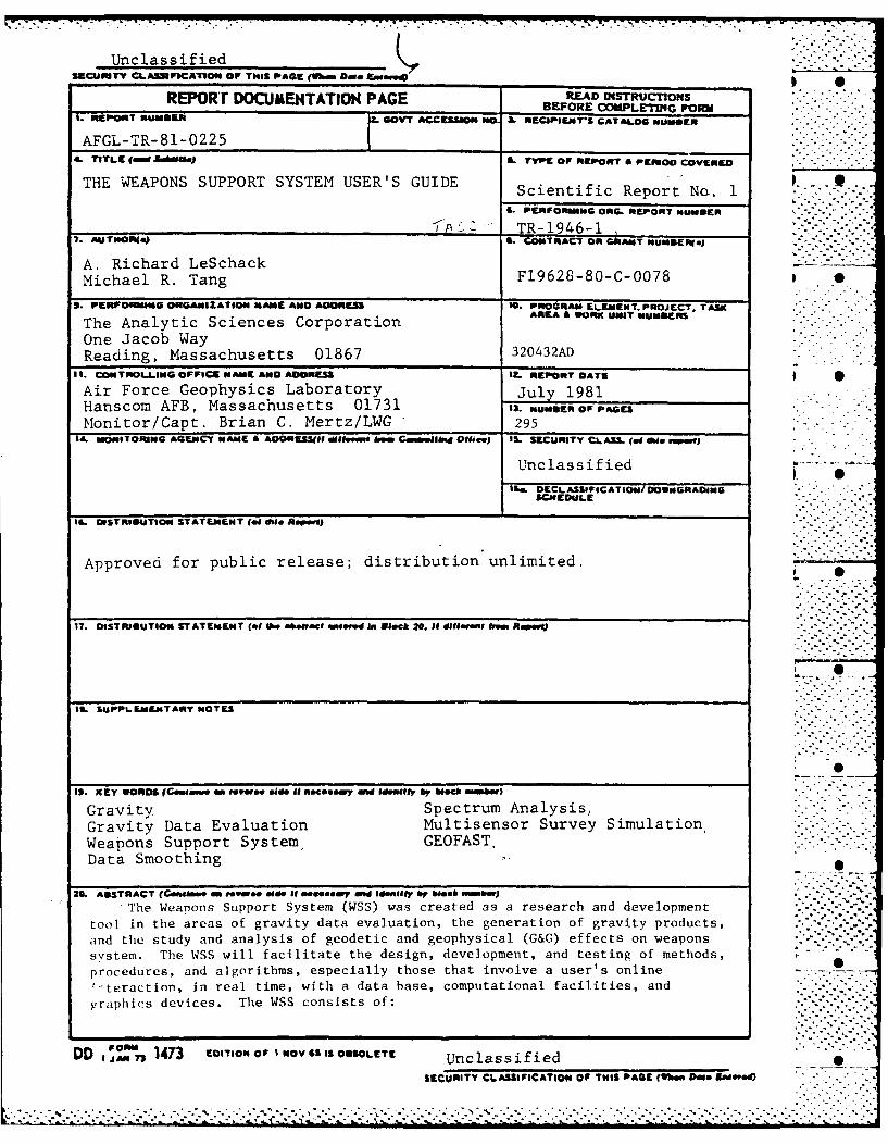
Approved for public release; distribution unlimited.

17. OISTRIOUTION STATEMENT (.4 IA. absract metrd In Bieck 20. UI dlIf ru b RMe) O-&-

111, SUPPLEMENTARY NOTES

I9. 9EY WORDS (Consomme on fre ide OfnLi sr MOO W1 I&ANWERY 67 block amber)

Gravity Spectrum Analysis,Gravity Data Evaluation Multisensor Survey SimulationWeapons Support System. GEOFAST.Data Smoothing

20& ABSTRACT (Ctman ew ee de Of ueeenry mos d entuatr by bseei onmber)

The Weapons Support System (WSS) was created as a research and development

tool in the areas of gravity data evaluation, the generation of gravity products,and the study and analysis of geodetic and geophysical (G&G) effects on weaponssystem. The WSS will facilitate the design, development, and testing of methods,procedures, and algorithms, especially those that involve a user's online

1-teraction, in real time, with a data base, computational facilities, andp!rdThics devices. The WSS consists of:

DD g rs1473 EDTIONro or I NOV GS IS OBSOLETE Unclassified

SZCURITY CLASSI1FICATION OF THIS PAGE (112m Dime Entemoe

BLOCK 20 (Contd)

S -HARDWARE: - a carefully integrated combination of powerfulminicomputer with associated peripheral devices, including

user terminals and a color graphics display unit

SYSTEMS SOFTWARE: - a time-sharing virtual memory operating

system to support a multiuser environment.

APPLICATIONS SOFTWARE: - custom programs developed for theWSS, in these four application areas:

Evaluation of gravity data

Data smoothing and analysis,Multisensor survey simulation,Rapid gravity field estimation (GEOFAST),

Accession For

NTIS GRA&IDTIC TABUnannounced

Justification

Distribution/ .

Availa ility CodesjAvail and/or

Dist Special .-

A-1

Mr.

. - .. ,°...-..... .. • . . . . .. . . . . -'..--.. . . . . .

'9,.. .

TABLE OF CONTENTS

Page

No.

List of Figures v 0

List of Tables vi

I. THE WEAPONS SUPPORT SYSTEM USER'S GUIDE 1-11.1 Introduction 1-11.2 The WSS Hardware 1-21.3 The WSS Systems Software 1-31.4 The WSS Applications Software 1-6

2. USER'S GUIDE FOR THE GRAVITY DATAEVALUATION CAPABILITIES 2-1 ""2.1 Overview of the Gravity Data

Evaluation Capabilities 2-12.2 Preprocessing Requirements 2-22.3 The Scatter Plot Program 2-4

2.3.1 Purpose and Scope 2-42.3.2 Program Limitations 2-42.3.3 Running the Scatter Plot Program 2-5

2.4 File Editing and Manipulation Utilities 2-10 -2.4.1 Introduction 2-102.4.2 Interactive Text Editor 2-112.4.3 SORT/MERGE Facility 2-12

2.5 The Contour Plot Program 2-132.5.1 Purpose and Scope 2-13 -

2.5.2 Program Limitations 2-142.5.3 Running the Contour Plot Program 2-14

2.6 The Three-Dimensional Surface Plot Program 2-212.6.1 Purpose and Scope 2-212.6.2 Program Limitations 2-212.6.3 Running the Three-Dimensional Surface

Plot Program 2-232.7 Robust Estimation and Statistical Plot Program 2-27

2.7.1 Purpose and Scope 2-272.7.2 Program Limitations 2-272.7.3 Running the Statistical Plot Program 2-27

2.8 Ocean Track-Crossing Adjustment Programs 2-352.8.1 Purpose and Scope 2-352.8.2 Program Limitations 2-362.8.3 Ocean Track-Crossing Adjustment

Program Descriptions 2-372.8.4 Running the Ocean Track-Crossing

Adjustment Programs 2-4"

iii ''

: .. ....'-.'- -.- .. : .'-,'. '- '....' .'. '. ..' ',.-. .-.' " v -, "-. ., ..".. -" .'.. -. -." ..- . .. " " ' " .- -" ' ," ' ,i"

TABLE OF CONTENTS (Continued)

PageNo.

2.9 ERROR AND DIAGNOSTIC MESSAGES 2-482.9.1 General Error Messages 2-482.9.2 Scatter Plot Program Error Messages 2-502.9.3 Statistical Plot Program Error Messages 2-502.9.4 Ocean Track-Crossing Adjustment

Program Error Messages 2-51

3. USER'S GUIDE TO THE SMOOTHING AND SPECTRUMANALYSiS PROGRAMS 3-13.1 Introduction 3-13.2 Data Formats 3-33.^ Data Selection (Program GETDATA) 3-43.4 Autoregressive Spectrum Analysis (Program AR) 3-83.5 Periodogram Spectrum Analysis and Plotting

(Programs FFT and PLOTFFT) 3-133.6 Error and Diagnostic Messages 3-22

4. USER'S GUIDE TO THE MULTISENSOR SURVEYSIMULATION SOFTWARE 4-14.1 Applications of the Multisensor Survey

Simulation Software 4-14.2 Running the MULTISENS Program 4-2

4.2.1 Running the TRANSFER Phase 4-84.2.2 Running the GRAVITY Phase 4-124.2.3 Running the IMPACT Phase 4-404.2.4 Sensitivity Runs 4-414.2.5 File Format Requirements 4-444.2.6 Interfaces for User-Written Subroutines 4-48

4.3 Running the MULTIJOB Program 4-504.3.1 Requirements and Limitations 4-514.3 2 Input Formats 4-514.3.3 Program Execution 4-554.3.4 Error Messages 4-64

4.4 Running the MULTIPLOT Program 4-664.4.1 Preprocessing Requirements and Limitations 4-664.4.2 Program Execution 4-664.4.3 Error Messages 4-71

. USER'S GUIDE TO THE GEOFAST ESTIMATION SOFTWARE 5-15.I Overview of GEOFAST Capabilities 5-1i.2 GEOFAST Programs 5-3

5.2.1 The GEOFAST Command Program 5-45.2.2 The GEOCOV3 Program 5-55.2.3 The GEOEST3 Program 5-125.2.4 The GEOPLOT Command Program 5-17

iv

~° .

TABLE OF CONTENTS (Continued)

PageNo.

APPENDIX A LIST OF MULTISENS INPUT PARAMETERS A-1

APPENDIX B DESCRIPTION OF NAMELIST FACILITY B-1

REFERENCES R-1

V

_"7777-

LIST OF FIGURES

Figure PageNo. No.

1.2-1 Weapons Support System Architecture 1-3

2.5-1 Typical Contour Plot 2-15

2.6-1 Typical Surface Plot 2-22

2.8-1 Ocean Track-Crossing Adjustment Worksheet 2-47

4.2-1 MULTISENS Functional Macrodiagram 4-3

4.2-2 Input Control File 4-7

4.2-3 Frequency Pairs for Transfer Function Table 4-9

4.2-4 Frequency Domain Grid for Evaluation of Residuals 4-16

4.2-5 Frequency Domain Grids for Multiple Scans 4-18

4.3-1 Samples of Individual Questions Inputs 4-52

4.3-2 Sample of Table Input Parameter Prompting 4-54

4.3-3 Sample of Input Verificatlion Mode Responses 4-56

5.1-1 Overview of the GEOFAST Algorithm 5-2

5.2-1 Sample GEOFAST Run 5-6

5.2-2 GEOFAST Covariance Phase 5-9 -

5.2-3 Time and Storage Variation With Bandwidth 5-9

5.2-4 GEOFAST Estimation Phase 5-13

vi-

2-5 Frequncy Doman.Gri....r.M....p..Scans.-18..-.-

4 3-1 Sampies of.....................s In ut 4-52. '. -

-. -------------- ~ r . . . . -. -

LIST OF TABLES

Table PageNo. No.

2.9-1 Warning Messages 2-49

4.2-1 Predetermined Value of Integration ControlParameters for the R.MS and AREAMEAN Modes 4-20

4.2-2 Gradiometer Survey Parameters 4-37

5.2-1 Input Parameters for GEOCOV3 5-10

5.2-2 Input Parameters for GEOEST3 5-14

Viii

1. THE WEAPONS SUPPORT SYSTEMUSER'S GUIDE

1.1 INTRODUCTION .

The Weapons Support System (WSS) was created as a

research and development tool in the areas of gravity data

evaluation, the generation of gravity products, and the study

and analysis of geodetic and geophysical (G&G) effects on wea-

pons systems. The WSS will facilitate the design, development,

and testing of methods, procedures, and algorithms, especially

those that involve a user's online interaction, in real time,

with a data base, computational facilities, and graphics devices.

At delivery time, the WSS consists of:

0 HARDWARE:- a carefully integrated combina-tion of powerful minicomputer with asso-ciated peripheral devices, includinguser terminals and a color graphics dis- -

play unit

0 SYSTEMS SOFTWARE:- a time-sharing virtualmemory operating system to support amultiuser environment

* APPLICATIONS SOFTWARE:- custom programsdeveloped for the WSS, in these fourapplication areas:

Evaluation of gravity dataData smoothing and analysisMultisensor survey simulationRapid gravity field estimation (GEOFAST)

This introductory section gives an overview of the

WSS hardware, the systems software, and the four major areas

of application software, from the point of view of the user of

......... .. .I - i ."7:

. . . . .. ._

the WSS. Detailed operating instructions for each of the soft-

ware areas follow the introduction.

1.2 THE WSS HARDWARE

The WSS hardware is based on a Digital Equipment Cor-

poration (DEC) VAX-11/780 computer with 1.5 megabytes of high-

speed storage. Additional memory is provided by two disk

storage units:

" The DEC RM03 disk unit with a capacityof 67 megabytes

" The System Industries 9466 disk unitwith a capacity of 300 megabytes.

The magnetic tape unit is a DEC TEl6, which operates at a speed

of 45 inches per second. A Printronix P600 line printer, with

a capacity of 600 lines per minute, also serves as a medium-

resolution plotter. The system uses a DECwriter III (LA 120)

as the operator's console. The architecture is shown in

Fig. 1.2-1.

Most user interaction will be with the five terminal

devices currently supported by the WSS. Four of these are

video data terminals, consisting of a keyboard and a DEC VTOO

vidoo display unit. Users enter data and commands, create and

run programs, and view files and program output at these termi-

nals. The fift.h device is the Lexidata Display Unit, a color

graphics monitor which can display maps, contour plots, and

,iany other kinds of graphical out put. Associated with the

Lexidata unit is a t rackbal I cont rol device, to facilitate

user 'ont rol of and interact ion with the displayed data. Any.\

output displayed on the screen ot the Lexidat a unit can be

1-2

R-62069

120 CPSCONSOLE [ I VAX-11/780 R 67 MBYTETERMINAL DISK

VAX/VMS

1.5FLOPPY DISK Ro------.- MEGABYTES q 9466 300 MBYTE

DISK

1.5 MBYTE 600 LPMECC MOS M P PRINTER/PLOTTER

45 IPS COLOR GRAPHICSMAGNETIC 4 0 EIDT DISPLAY AND

TAPE DRIVE 3401TRACKBALL

VT 100 VT100 VT 100 VT 100

D KEYBOARD KEYBOARD KEYBOARD

Figure 1.2-1 Weapons Support System Architecture

printed (although in black and white only) on the P600 line

printer as a permanent hard copy.

1 .3 THE WSS SYSTEMS SOFTWARE

The VAX-l1/780 computer and its associated peripheral

devices operate under the control of the VAX/VMS Operating

I -- .

2 -Typing a 2 will invoke the cursor on thegraphics terminal and allow the user toselect individual points. To select apoint, the user moves the cursor with thetrackball over a point, and toggles theblue switch. The selected point will bemarked in red. If there are several pointsnear the cursor, the program will selectthe point nearest to the center of thecursor. The record in the gravity filecorresponding to the selected point willbe displayed at the VT100 terminal. Theuser will then have the option of savingthe point in a separate file. Additionalpoints can then be identified by movingthe cursor and toggling the blue switch.To terminate this option, the user shouldtoggle switch A (i.e., the left-most whiteswitch).

3 - Typing a 3 will allow the user to selectall points within a rectangular region onthe scatter plot. Using the trackball,the user moves the cursor to one cornerof the desired region and toggles theblue switch. A red "+" will appear onthe graphics terminal. The user thenmoves the cursor to the diagonally oppositecorner of the region, and again togglesthe blue switch. Another "+" will appearat the point, and the rectangular regionwill be drawn using the two marked points.The points within the region will be markedin red, and a listing of the records ofall the selected points will be displayedon the VT100 screen. The user will havethe option of saving these points in aseparate file. More regions can then bedrawn by repeating the same steps. Toterminate this option, the user shouldtoggle switch A (i.e., the left-most whiteswitch).

4 - Typing a 4 will allow the user to selectentire tracks of data. This feature ismost useful when analyzing ocean data,where the data tend to lie along tracks.As in selecting points within a rectangularregion, the user employs the cursor toThe selected points will be marked inred, and they will also be listed at the

2- -.

-- .:I,.-----------------•. .

O

Quit - Typing Quit (or Q) will cause the program toterminate.

If the user selects the zoom, scroll, and point selec-

tion option, the VT100 terminal screen will clear, and a map

legend, which lists the source numbers and cor:esponding letters 0

of the alphabet, will appear. The following menu will then be

displayed on the VT100 screen:

ENTER 1 - ZOOM AND SCROLL2 - USE CURSOR TO SELECT INDIVIDUAL POINTS3 - USE CURSOR TO SELECT POINTS WITHIN

A RECTANGULAR REGION4 - USE CURSOR TO SELECT ENTIRE TRACKS5 - USE CURSOR TO IDENTIFY INTERSECTION POINTS

99 - TO EXIT FROM THE PROGRAM

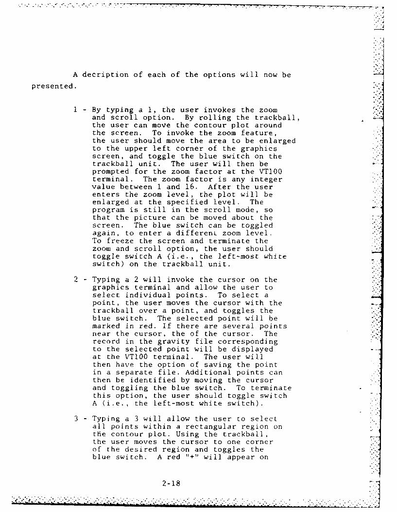
A description of each of the options will now be

presented.

1 - By typing a 1, the user invokes the zoomand scroll option. I- rolling the track-ball, the user can move the scatter plotaround the screen. To invoke the zoomfeature, the user should move the area tobe enlarged to the upper left corner ofthe graphics screen, and toggle the blueswitch on the trackball unit. The userwill then be prompted for the zoom factorat the VT100 terminal. The zoom factoris any integer value between I and 16.After the user enters the zoom level, theplot will be enlarged at the specified. -

level. The program is still in the scrollmode, so that the picture can be movedabout the screen. The blue switch can betoggled again, to enter a different zoomlevel. To freeze the screen and terminatethe zoom and scroll option, the user shouldtoggle switch A (i.e., the left-most whiteswitch) on the trackball unit. p

2-7

..........................................

After reading the gravity file, the program will prompt

the user for several inputs regarding latitude and longitude

limits for the plot, plot title, and whether the user wants

grid lines on the plot. All of the prompts have default values,

which the user can select by pressing only the RETURN key.

The scatter plot is drawn using letters of the alphabet

to represent data points from different sources. The major

political boundaries and coastlines which lie within the limits

of the scatter plot are drawn in red, and the latitude and

longitude grid lines are drawn in blue.

When the scatter plot is completed, the following

menu will appear on the VT100 screen:

TYPE (CR> - TO ZOOM, SCROLL AND IDENTIFYPOINTS WITH THE CURSOR

Replot - TO CREATE NEW PLOTPrint - TO GET A HARD COPY OF PLOTQuit - TO HALT PROGRAM EXECUTION

When an option is selected, only the first letter of

the user's response is examined. Hence, typing any character

string that starts with P will produce a hard copy of the plot.

A description of each option will now be given.

"CR> - Typing the RETURN key will allow the user tozoom, scroll, and select points using the cursor.Further details will be presented below.

Replot - By typing Replot (or R), the user can create anew plot on the graphics terminal. The userwill be prompted for new latitude and longitudelimits, and a new title.

Print - Typing Print (or P) will cause the scatter ploton the graphics terminal to be printed on theline printer. The user will then be asked toselect again from this same menu.

2-6

• ~ ~ ~~.. . . .. . . . . . . . . . . . . . . .. .. .. .. ,. .... _.. .

-. -~-. -' . -~ C.~t wr• -,.

Since the program uses the letters of the alphabet to distinguish

different sources, a maximum of 26 unique sources can be identi-

fied within a given region.

2.3.3 Running the Scatter Plot Program

To run the scatter plot program, the user types the

following command:

RUN SCATTER

The user will then be prompted to enter the name of

the file containing the gravity survey data to be examined.

The file name must include all qualifiers to identify the file

uniquely. A complete file specification has the following

format:

device: (directory] filename.type;version

The punctuation marks (colons, brackets, periods) are required

to separate the various components of the file specification.

If the input file is on the same directory as the user, only

the filename and type need to be specified. The default file

type is DAT, and if no version number is given, the file with

the highest version number is used. Volume 2A of the VAX/VMS

Reference Manuals contains a complete description of file

specification.

If the word QUIT is typed for the input file name,

the scatter plot program will stop execution and return con-

trol to VMS. The user should note that if the word QUIT is

typed for many of the input prompts, the program will ter-

minate and return control to VMS.

2-5

. . . . . . . ... . . . . .-

Before using any of the programs in the gravity data

evaluation section, the user should make sure that the gravity

file to be examined is in the WSS online format.

2.3 THE SCATTER PLOT PROGRAM

2.3.1 Purpose and Scope

The purpose of the scatter plot program is to display

on the Lexidata graphics terminal the geographic locations of

the gravity stations in a file containing gravity survey data.

The scatter plot is superimposed on a map showing major poli-

tical boundaries and coastlines. The map is drawn using a

Mercator map projection. Both land and ocean survey data can

be displayed using this program, and multiple sources within

the same region are distinguished using different letters of

the alphabet. The program is also set up to invoke the cursor,

which can be used to identify individual points or subsets of

points. The scatter plot program is run interactively from

one of the VT100 terminals, and it requires the user to respond

to several prompts and menu selection options.

2.3.2 Program Limitations

Since the scatter plot program requires the use of

the Lexidata graphics terminal, the user should make sure that

the graphics terminal is available before running the program.

The user should also make sure that all the toggle switches on

the trackball unit are in the OFF position.

The scatter plot program handles files with up to

5000 points. Larger files should be separated into smaller

subfiles before processing with the scatter plot program.

2-4

• i -. 2.'. .. . , i i- -12< -' .2. 2 )-2... ).) -i.i- .2.. -2 . -.. :? =2 "'-.-...... ... .'--. ."."-.. .... "-.. '- . : 22.

convert from the card format to the WSS online format. This

utility program, called REFORMAT, is included as part of the

gravity data evaluation software. The program will first read

the data stored in the 80 column card format. It will then

allow the user to select subsets of the data based on:

* Geographic latitude/longitude boundaries

* Source identification number

* Any combination of the two.

The utility program will then create a data file containing

the chosen subset of points in the WSS online format.

All of the programs which are part of the gravity

data evaluation software use as input any file which is in the

WSS online format. The WSS online format consists of the

following data fields:

* Source number

* Latitude (decimal degrees)

* Longitude (decimal degrees)

* Elevation (meters)

0 Observed gravity (less 976,000 mgal)

0 Free-air anomaly (mgal)

* Bouguer anomaly (mgal).

The file, in WSS online format is read by the various

programs using a formatted READ statement. The format for the

READ statement is given by:

FORMAT(15,2FI0.4,F8.1,F8.2,2F7.i)

2-3

7.. o .,' m T ' ,- . . - , m -. - . . , - . . , - , _. - " " -_ " .' -., . . ,' ' :

* The scatter plot program

* File editing and manipulation utilities

* The contour plot program

• The three-dimensional surface plot program

• Robust estimation and statistical plotprogram

0 Ocean track-crossing adjustment programs

The Gravity Data Evalution User's Guide is organized

in the following manner. The first section will describe the

formatting requirements for the data files which will be proc-

essed by the gravity data evaluation programs. The next six

sections will present detailed descriptions of how to imple-

ment the major sections of the gravity data evaluation soft-

ware. The final sedtion lists the error and warning messages

which may occur during execution of the evaluation programs.

2.2 PREPROCESSING REQUIREMENTS

The Weapons Support System uses two different data

formats for storing and processing gravity survey data. First,

the WSS can read and store data from the DoD Gravity Library -_

in the standard 80 column card format. For ease of use, how-

ever, a subset of the 80 column card format is commonly used

as input to the gravity data evaluation software. This data

format is called the WSS online format.

One of the implications of using the two different

data formats, is that even if the 80 column card format should

change, the WSS online format need not. However, the use of

two data formats means that a utility program must be used to

2-2

. . . . . .

.: : - - ' m - -- Y ' 9 I. LII"- .°.

2. USER'S GUIDE FOR THE GRAVITY DATA EVALUATION SOFTWARE

2 OVERVIEW OF THE GRAVITY DATA EVALUATION CAPABILITIES

The gravity data evaluation software is a collection

of tools designed to assist the evaluator in the various tasks

involved in analyzing gravity survey data. These tasks include:

* Elimination of erroneous and redundant

data

* Verification of gravity base station

* Adjustment of systematic inconsistenciesbetween sources

* Identification and correction of recover- -able errors

* Assignment of accuracy measures to eachsource.

The various programs which make up the gravity data

evaluation software make extensive use of the Lexidata graphics

terminal. The graphical displays are extremely useful in that

they provide the evaluator with a quick-look capability for _

making rapid decisions concerning the data. However, these

progr, ,,s also rely heavily on the evaluator's judgment and

experience.

The gravity data evaluation software is divided into

major sections. They are:

2.1

,.:.-.-.- .°.:. . --.-..-... ..----.. . ........ ..... ...... .......... ...-. '..°.- ' - : - , . .. = = .' . " " " " , " ' . ' ' . . ' . ' '

-" " • - " " -. . . ' - ' . - . .' -' . . - ' ' " . " " ' -

capabilities of the multisensor surveysimulation program .

* Running The MULTISENS program -- showingthe user how ro run the multisensor Eurveysimulation program

& Running The MULTIJOB Program -- showing 0the user how to create the job streamrequired to run MULTISENS

* Running the MULTIPLOT Program -- showingthe user how to generate plots of MULTISENSresults. P

The Geofast Estimation Software section of the WSS

User's Guide is organized as follows:

* Overview -- describing, in general terms,the capabilities and features of theGEOFAST package

* Program Execution -- showing the userhow to run the interactive front endprogram (GEOFAST) that prompts for re-quired input parameters and sets up thebatch jobs to do GEOFAST estimation, andexplaining, in summary form, the opera-tion of the two components of the estima-tion system: - GEOCOV3, which does pre-processing of covariances and carries outthe transformation to the frequency domain;and GEOEST3, which uses the output filesgenerated by GEOCOV3 to compute the re-quired estimates .

0 GEOPLOT -- describing the use of theinteractive program (GEOPLOT), whichdisplays the results of GEOFAST runs.

1-9,:7.:1

the various operations involved in the selectionof tracks, determination of gravity values atthe intersection points, computation of trackadjustments, and application of the computedadjustments to the gravity data file.

The section concludes with a summary of possible error messages

that the user may encounter.

The Spectrum Analysis and Smoothing Software section

of the WSS User's Guide is organized as follows:

* Introduction -- describing, in general -"

terms, the four programs that are availablefor data smoothing and spectrum analysis

& Data Formats explaining the standardWSS time series data file conventions

* Data Selection -- showing the user how

to run the program that examines datafiles, selects subsets, smooths, andresamples

0 AR Modeling -- showing the user how torun the program that carries out autore-gressive modeling and plots power spectraand coherency

* Periodogram Spectral Analysis And Plotting --

showing the user how to run the program(FFT) that carries out periodogram analysison the master data file or a selectedsubset, creating an averaged periodogramwith associated error statistics; andthe program (PLOTFFT) to generate period-ogram plots.

The Multisensor Survey Simulation Software section of

the WSS User's Guide is organized as follows:

• Applications Of The Multisensor SurveySimulation Software -- describing, ingeneral terms, the various options and

1 -8 .

S. .-. ,-, :j-::'.)i;(i:;i) ii,. ( :.: ( i -_.-i,(:i."i-F ,:'(" ; ..- . . . . . .. . .-.- ".-.'-V -.. '.- ,' .-. " -'."-.". -'..-,. .-. , -... .. '.

'0

control to the VAX/VMS operating system by entering QUIT as

a response to most interactive prompts.

The User's Guide is intended to be a system introduc-

tion and a working guide for use during terminal sessions.

A brief overview will now be given for each of the WSS applica-

tions software functions.

The Gravity Data Evaluation Software section of the

WSS User's Guide is organized as follows:

• Overview -- describing the gravity dataevaluation software in general terms

• Preprocessing Requirements -- explaining thestandard data format used for the point gravityfiles

" Scatter Plotting -- showing the user how to runthe program (SCATTER) that implements thescatter plotting features, including zoom,scroll, and the use of the cursor to selectindividual points and points within arectangular area

* File Editing and Manipulation -- showinghow to use the features of the VAX/VMSsystem editor (EDT) to accomplish fileediting, using the common station compareas an example

" Contour Plotting -- showing the user how to run 0the program (CONPLOT) that generates a labeledcontour plot on the Lexidata Graphics Terminal

* Three-Dimensional Plotting -- showing the userhow to run the program (SURPLOT) that generateslabeled three-dimensional plots

* Robust Estimation and Statistical Plotting --

showing the user how to run the program(STATPLOT) that implements the various robustestimators and generates statistical plotslike the QQ Plot

0 Track Crossing Adjustment Tools -- showing theuser how to run the four programs that implement .. .

1 - 7 ::"-1-7.°°-

e ° . . - ° . °. - . . ° . .. ° . ° , , - - . .o o • . . . . . . • . .. . . .. . . , - .

The TASC Graphics Software Package originated with

the National Center for Atmospheric Research and has been exten-

sively modified by TASC for use with the WSS. It provides the

following features:

0 Automatic generation of various kinds of

graphs

0 Contour plotting

* Three-dimensional plotting

* Map generation

0 Generation of halftone pictures

* Velocity displays

0 Generation of characters and printedtitles.

The TASC Graphic Software Package is documented in

Ref. 7.

1.4 THE WSS APPLICATIONS SOFTWARE

The WSS Applications Software includes the following

major capabilities, each of which is documented in detail in

the sections to follow:

0 Gravity Data Evaluation

* Spectrum Analysis and Smoothing Software

0 Multisensor Survey Simulation Software

6 GEOFAST Estimation Software.

During execution of WSS application software, the

user may stop execution of the application software and return

1-6 -

These are used extensively by the WSS applications programs to

be described in this User's Guide. Th, are also available to

WSS users who will be writing their own programs.

IMSL, a carefully tested and documented collection of

495 FORTRAN programs, includes the following categories:

* Analysis of Variance-

* Basic Statistics

0 Categorized Data Analysis

* Differential Equations and Quadrature

* Eigensystem Analysis

* Forecasting, Time Series, and Transforms

* Random Numbers

* Interpolation, Approximation, and Smoothing

* Linear Algebraic Equations

* Mathematical and Statistical SpecialFunctions

• Nonparametric Statistics

" Observation Structure and MultivariateAnalysis

* Regression Analysis 0

* Sampling

• Utility Functions

0 Vector and Matrix Arithmetic 9

0 Zeros, Extrena, and Linear Programming.

The IMSL programs are described in a three-volume reference

manual published by International Mathematical and Statistical

Libraries, Inc., delivered with the system.

1-5- °

....................-......".'.-'--.','.".--- ..-. .- -': Y. .-'>-'"''--. -'...-- -. ",., . . "- .-•'.-.'I

System. Version 2.2, which is designed to permit the simul-

taneous use of the computer and associated hardware by many

users. The operating system is described in summary form, at

the level required by the WSS user, in a Digital EquipmentCorporation document entitled VAX/VMS Primer, copies of which

will be delivered with the WSS. The WSS user will find baFic

instructions in the Primer for logon and logoff procedures,

and for using the VT1O0 terminal to communicate with the sys-

tem. Beyond these basic concepts, most WSS users will require

knowledge of only a few features of the operating system in

order to use the existing WSS capabilities, since detailed and

s ,tvf-contained directions are provided for each applications

program in this User's Guide. The most important of these

teatures for the WSS user is the EDITOR, a powerful and easy-

to-use tool for the creation, examination, and modification ,,f

files -- a term that includes data as well as programs. The

use of EDIT commands to manipulate gravity data files in the

cntext of gravity data evaluation is described below in sec-

*tion 2.2.4 (File Editing and Manipulation).

Detailed documentation of the VAX/VMS Operating Sys-

t,,m is available in the form of a multivolume set of manuals.'l1w Primer, as well as the Information Directory and Index in

V,1um One of the VAX/VMS Documentation, will direct the user

to the appropriate source of detailed information about any

as.pect of the Operating System.

Also included under the heading of systems software

are the following software packages:

- The International Mathematical and Statis-tical Library (IMSL)

0 The TASC Graphics Software Package.

L-L.

-' . . ' , . ' . . . . . . . . - . . . . . .

VTIOO terminal. The user will have theoption of saving them. To terminate thisoption, the user should toggle switch A(i.e., the left-most white switch).

5 - Typing a 5 will allow the user to deter-mine the coordinates of track intersectionpoints. Again, this is most useful when

analyzing ocean data. The user shouldmove the cursor over the intersectionpoint and toggle the blue switch. Thelatitude and longitude coordinates of theintersection point will appear on theVT100 screen. Further intersection pointscan then be determined. To terminatethis left-most white switch).

99 - Typing a 99 will cause the program toterminate.

Note that for each of the user-selected options, the

user terminates an option by toggling switch A. The user menu

selection options will then appear on the screen. Before selec-

ting another option, the user should make sure that switch A

is in the OFF position.

If an invalid switch is toggled during execution of

any of the user selected options, the following message will

appear on the screen:

USER ERROR *AN INVALID SWITCH HAS BEEN TOGGLEDRESET TOGGLE SWITCH AND TRY AGAIN

The user should move the invalid switch to the OFF position

before toggling the correct switch.

2-9

' :.:.:....JL ..... : .: : : : - / :: : " : " " " -

L

2.4. FILE EDITING AND MANIPULATION UTILITIES

2.4.1 Introduction

The VAX/VMS operating system has an extensive set of

commands for editing and manipulating data files and user pro-

grams. These commands are part of the Digital Command Language

(DCL). The DCL command language contains commands for perform-

ing such operations as:

* Changing and/or modifying files

* Printing files on the line printer

0 Deleting one or more files

0 Copying sections of one file into anotherfile

0 Sorting files on specified fields.

The various DCL commands are fully documented in Vol-

ume 2A of the VAX/VMS Reference Manuals. The documentation is

also available at the VT100 terminal by use of the HELP commaind.

To invoke the HELP command, the user simply types the word

HELP, followed by the command for which more information is

required. The HELP command will respond with a summary of the

format of the particular command or a list of the command's

valid qualifiers. For example, to obtain more information

about the COPY command, the user should type:

HELP COPY

The system responds by displaying at the terminal a summary of

the COPY command and keywords to enter as parameters to the

2-10

HELP command to obtain additional information. As an example,

if the user types:

HELP COPY/EXTENSION

the system will respond with information concerning the exten-

sions to be added to the output file. If the user enters:

HELP COPY QUALIFIERS

the HELP command will display a description of each of the

COPY command qualifiers.

Two of the file manipulation utilities which are used

very frequently are the interactive text editor and the sort-

ing facility. A description of these two utilities will now

be presented.

2.4.2 Interactive Text Editor

The interactive text editor allows the user to examine,

create, and/or modify data files or user programs from the

VT100 terminal. The VAX/VMS operating system has two inter-

active text editors. They are called SOS and EDT. The SOS

editor is a line editor, while the EDT editor is a full-screen

editor. The EDT editor is the more useful of the two. Com-

plete documentation for both of these editors is given in

Volume 3A of the VAX/VMS Reference Manuals.

The easiest way to learn how to use the EDT editor is

to run the EDT Editor Computer Aided Instruction minicourse,

which is called EDTCAI. This minicourse is presented inter-

actively at the computer terminal. The computer will display

2-11

. . ,

information about the EDT editor on the VT100 terminal screen,

allow the user to practice entering EDT commands, and ask the

user questions about what has been learned. For more informa-

tion about running EDTCAI, the user should talk to the systems

manager.

2.4.3 SORT/MERGE Facility

The SORT/MERGE facility allows users of the VAX/VMS

operating system to reorder data files in either ascending or

descending order. The user can sort several files using the

same field, and then merge the files into one sorted file. The

user can run SORT/MERGE interactively from the terminal, as a

batch job, or as part of a user program.

The purpose of this section is to present a brief

introduction to some of the useful capabilities of the SORT/

MERGE facilities. The user should refer to Volume 3A of the

VAX/VMS Reference Manuals for a detailed description of the

various features in the SORT/MERGE program.

The SORT command has the following general form:

SORT/KEY=([qualifiers]) input-file(s) output-file

The qualifiers specify which data field is to be used as the

sort key. The user can specify up to 10 different input files,

which must exist either on the disk or magnetic tape. The out-

put file contains the sorted records.

For example, assume that the user has a WSS gravity

input file called SRCE4242.DAT. (See Section 2.2 for a descrip-

tion of the WSS online file format). To sort this file on the

elevation field, the user types:

2-12

* - '' .- ~ -'- ~ 1 ... -.I II-. w--. ~ - . . .---.-. .. ~.,J Z. . - r r vr r - - . . - -

SORT/KEY=(POSITION=26,SIZE=8) SRCE4242 .DAT SORT.DAT

The output file, SORT.DAT, will contain all the records of the

file SRCE4242.DAT sorted by elevation in ascending order.

If more than one input file is specified, the input

files will all be sorted on the specified field, and then merged

into a single sorted file. This could be used to facilitate a

Common Station Compare. For example, if the user has two files

of gravity survey data covering the same region, FILEI.DAT and

FILE2.DAT, then the following command:

SORT/KEY=(POS=6,SIZE=1O)/KEY=(POS=16,SlZE=1O)-FILE1.DAT,FILE2.DAT COt4MON.DAT

will first sort the two input files by latitude and longitude,

and then merge the two sorted files into COMMON.DAT. Hence,

pairs of points which are geographically close to each other

will appear as sequential records in the output file.

Similarly, if several data files have already been .

sorted on the same field, they can be merged into a single

sorted file using the MERGE command. The user should look in

the reference manual for details on the MERGE command.S

2.5 THE CONTOUR PLOT PROGRAM

2.5.1 Purpose and Scope IL

The purpose of the contour plot program is to display

on the Lexidata graphics terminal a contour plot of a specified

data field from a file containing gravity survey data. The

program is set up to overlay the contour plot with a scatter

2-13

1.. 7._'-..-'-'.-".- - _ . . . '. ''- ..

-.. . " ".. . -.". .- ". .. ". .. ." ..", ..... . . . . . ... . .-. ... ."... .... , .'. o. .. ,, ,".". " " " . ' ? " .

plot, which shows the geographic locations of the individual

gravity stations of the gravity survey file. Both land and

ocean survey data can be displayed using this program, and the

data need not be evenly spaced. The program is also set up to

invoke the cursor to identify individual points or subsets of

points. The contour plot program is run interactively from

the one of the VT100 terminals, and it requires the user to

respond to several prompts and menu selection options.


Since the contour plot program requires the use of



Also, the user should make sure that all the toggle switches

located on the trackball unit are in the OFF position.

The contour plot program handles files with up to

5000 points. Larger files should be separated into smaller

subfiles before processing with the contour plot program. The

contour plot program also requires a minimum of two data points.

However, to ensure that the contour plot adequately represents

the data field, the file should contain at least 10 data points.

2.5.3 Running the Contour Plot Program

To run the contour plot program, the user types the " -

following command:

RUN CONPLOT

The user will then be prompted to enter the file name

containing the gravity survey data to be examined. The file

name must include all qualifiers to identify the file uniquely.

A complete file specification has the following format:

2-14-.--- -''v-'-.-,' .. ". .-....-.-.. •..... . ,.............. .......... ii'

device: [ directory] filename.type ;version



If the input gravity file is located on the same directory as

the user, only the filename and type need to be specified. The

default type is DAT, and if no version number is specified,

then the file with the highest version number is used. Volume

2A of the VAX/VMS documentation contains a complete description

of file specification.


the contour plot program will stop execution and return control .

to VMS. The user should note that if the word QUIT is typed

for many of the input prompts, the program will terminate and

return control to VMS.

After reading the gravity file, the program will prompt

the user for inputs regarding latitude and longitude limits

for the contour plot. All of the prompts have default values,

which the user can select by pressing the RETURN key.

The user will then receive the following message at

the terminal: I

WHAT TYPE OF CONTOUR PLOT?TYPE E 1 ELEVATION PLOT

F 2 FREE-AIR ANOMALY PLOTB 3 BOUGUER ANOMALY PLOT

The default value is a contour plot of the Bouguer anomaly

field. The user can select the default by pressing the RETURN

key. .

2-15

:'-."-"°-. .i- .','" ;-.". ."-,L,.":'..'L.,...i . . .. .i.,. .L 2.i - - .. •. ........ , . .. ... v .. . . ..

The user is then requested to enter a title for the

plot. The default title is the input file name, but the user

may also wish to specify the field being contoured. That is,

a more useful title may be something like SOURCE 4242 BOUGUER

ANOMALY. The plot title must be less than 40 characters.

The following message will then appear on the screen:

DO YOU WISH TO SELECT YOUR OWN CONTOUR LEVELS?ENTER Yes OR NoDEFAULT -No :LET PROGRAM CHOOSE "NICE" CONTOUR LEVELS

If the user selects the default option, the program will select

the contour levels to be drawn. The program will select between

10 and 30 evenly spaced contour levels which will cover the

range of data values.

The user can specify the contour levels by typing

"YES" in response to the above prompt. If this option is

selected, the user will be prompted for a minimum contour level,

a maximum contour level, and the increment between the contour

levels. The user can specify the value 0.0 for the increment

value. This will cause the program to choose between 10 and

30 contour levels which lie between the maximum and minimum.

The contour plot is drawn so that the major contour

levels are in green and the minor contour levels are in red.

Positive contour levels are drawn as solid lines, while nega-

tive contours are drawn as dashed lines. Local minimum and

maximum are labeled on the contour plot with an L and H,

respectively. The geographic locations of the actual data

points are marked on the plot with blue 1'+"s.

When the contour plot is completed, the following


2-16

. . . . . .. . . . .. --

- ., -. ".", -

TYPE <CR> - TO ZOOM, SCROLL AND IDENTIFYPOINTS WITH THE CURSOR





A description of each option will now be given:

<CR> - Typing the RETURN key will allow the user to zoom,scroll, and select points using the cursor. Furtherdetails will be presented next.

Replot - By typing Replot (or R), the user can create a newplot on the graphics terminal. The user will beprompted for new latitude and longitude limits, adifferent data field, a new title, and new contourlevels. As before, default values are available forthe various prompts.

Print - Typing Print (or P) will cause the contour plot onthe graphics terminal to be printed on the lineprinter. The user will then be asked to select agai "from this same menu.

Quit Typing Quit (or Q) will cause the program toterminate.

If the user selects the zoom, scroll and point selec-

tion option, the following menu will appear on the screen:

ENTER 1 ZOOM AND SCROLL2 - USE CURSOR TO SELECT INDIVIDUAL POINTS3 -USE CURSOR TO SELECT POINTS WITHIN

A RECTANGULAR REGION4 NEW PLOT

99 -TO EXIT FROM THE PROGRAM

2-17

.,-., ',-.,-.-.,-.-.-.,.,..,.-,.-,.---.,-.-.-,.-..-,.-,.,.-,-,.-.... . . . ..,....-... .-... . ... . .-...-.. .. . .... .. ,...-

* .L

A decription of each of the options will now be

presented.

I - By typing a 1, the user invokes the zoomand scroll option. By rolling the trackball,the user can move the contour plot aroundthe screen. To invoke the zoom feature,the user should move the area to be enlargedto the upper left corner of the graphicsscreen, and toggle the blue switch on thetrackball unit. The user will then beprompted for the zoom factor at the VT100terminal. The zoom factor is any integervalue between 1 and 16. After the userenters the zoom level, the plot will beenlarged at the specified level. Theprogram is still in the scroll mode, sothat the picture can be moved about thescreen. The blue switch can be toggledagain, to enter a differenL zoom level.To freeze the screen and terminate thezoom and scroll option, the user shouldtoggle switch A (i.e., the left-most whiteswitch) on the trackball unit.

2 - Typing a 2 will invoke the cursor on thegraphics terminal and allow the user toselect individual points. To select apoint, the user moves the cursor with the -.

trackball over a point, and toggles theblue switch. The selected point will bemarked in red. If there are several pointsnear the cursor, the of the cursor. Therecord in the gravity file correspondingto the selected point will be displayedat the VTI00 terminal. The user willthen have the option of saving the pointin a separate file. Additional points canthen be identified by moving the cursorand toggling the blue switch. To terminatethis option, the user should toggle switchA (i.e., the left-most white switch).

3 - Typing a 3 will allow the user to selectall points within a rectangular region onthe contour plot. Using the trackball,the user moves the cursor to one cornerof the desired region and toggles theblue switch. A red "+" will appear on

2-18 -. -

I

the graphics terminal. The user thenmoves the cursor to the diagonally oppositecorner of the region, and again togglesthe blue switch. Another "+" will appearat the point, and the rectangular regionwill be drawn using the two marked points.The points within the region will be markedin red, and a listing of the records ofall the selected points will be displayedon the VT100 screen. The user will havethe option of saving these points in aseparate file. More regions can then bedrawn by repeating the same steps. Toterminate this option, the user shouldtoggle switch A (i.e., the left-most whiteswitch).

4 - By typing a 4, the user can create a newcontour plot on the graphics terminal.The user will be prompted for new latitude pand longitude limits, a different datafield, a new title, and new contour levels.As before, default values are availablefor the various prompts.




selection options will then appear on the screen. Before select-

ing another option, the user should make sure that switch A is

in the OFF position.

If an invalid switch is toggled during execution of ."



** USER ERRORAN INVALID SWITCH HAS BEEN TOGGLEDRESET TOGGLE SWITCH AND TRY AGAIN



2-19

..................................... -.. .

• s , -

2.6. THE THREE-DIMENSIONAL SURFACE PLOT PROGRAM


The purpose of the three-dimensional surface plot

program is to display on the Lexidata graphics terminal a sur-

face plot of a specified data field from a file containing

gravity survey data. Both land and ocean survey data can be

displayed using this program, and the data need not be evenly

spaced. The three-dimensional surface plot program is run

interactively from the one of the VT100 terminals, and it re-

quires the user to respond to several prompts and menu selec-

tion options.


Since the surface plot program requires the use of



The user should also make sure that all the toggle switches


The surface plot program handles files with up to

5000 points. Larger files should be separates into smaller

subfiles before processing with the surface plot program. The

surface plot program also requires a minimum of two data points.

However, to ensure that the surface plot adequately represents . -

the data field, the file should contain at least 10 data points.

2.6.3 Running the Three-Dimensional Surface Plot Program

To run the surface plot program, the user types the

following command:

RUN SURPLOT

2-20............................................ . .


containing the gravity survey data that are to be examined. 0

The file name must include all qualifiers to identify the file

uniquely. A complete file specification has the following

format:

device:[directorylfilename.type;version



If the input gravity file is located on the same directory as

the user, only the filename and type need to be specified. The

default type is DAT, and if no version number is specified,

the file with the highest version number is used. Volume 2A of

the VAX/VMS Reference Manuals contains a complete description

of file specification.


the surface plot program will stop execution and return control

to VMS. The user should note that if the word QUIT is typed

for many of the input prompts, the program will terminate and P

return control to VMS.

After reading the gravity file, the program will prompt --..'-

the user for inputs regarding latitude and longitude limits 5

for the surface plot. All of the prompts have default values,

which the user can select by pressing the RETURN key.

The user will then receive the following message at

the terminal:

WHAT TYPE OF SURFACE PLOT?TYPE 1 - ELEVATION PLOT

2 - FREE-AIR ANOMALY PLOT3 - BOUGUER ANOMALY PLOT

2-21 :

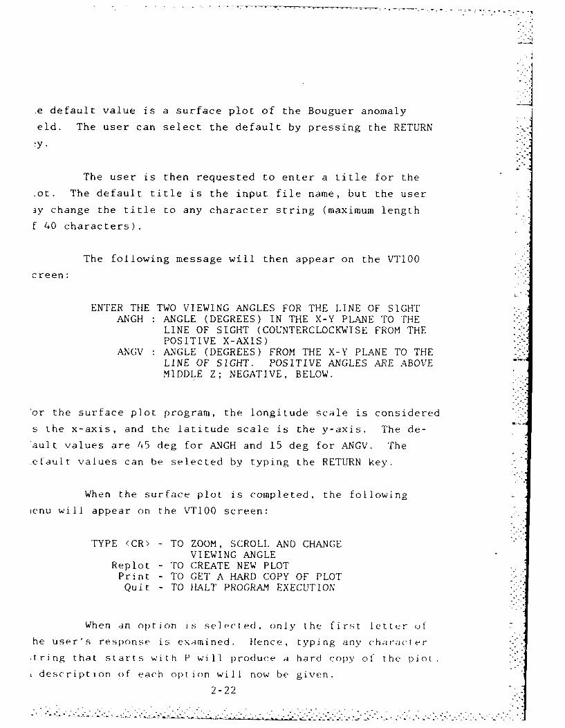
,e default value is a surface plot of the Bouguer anomaly

eld. The user can select the default by pressing the RETURN

.y.


ot. The default title is the input file name, but the user

ay change the title to any character string (maximum length

f 40 characters).

The following message will then appear on the VT100

creen:

ENTER THE TWO VIEWING ANGLES FOR THE LINE OF SIGHTANGH ANGLE (DEGREES) IN THE X-Y PLANE TO THE

LINE OF SIGHT (COUNTERCLOCKWISE FROM THEPOSITIVE X-AXIS)

ANGV ANGLE (DEGREES) FROM THE X-Y PLANE TO THELINE OF SIGHT. POSITIVE ANGLES ARE ABOVEMIDDLE Z; NEGATIVE, BELOW.

or the surface plot program, the longitude scale is considered

.s the x-axis, and the latitude scale is the y-axis. The de-

ault values are 45 deg for ANGH and 15 deg for ANGV. The

iefault values can be selected by typing the RETURN key.

When the surface plot is completed, the following

ienu will appear on the VT100 screen:

TYPE <CR) - TO ZOOM, SCROLL AND CHANGEVIEWING ANGLE


When an option is selected, only the first letter ot

he user's response is examined. Hence, typing any character

tring that starts with P will produce a hard copy of the plot.

description of each option will now be given.

2-22.. ........ ~~~~~~~~~~~~~~~~~~~.......................... ............. ........ ---.- : . ... ,. . ,.. ... :..,5.-.. ,"...'}i

in each segment using the cursor, andwrite the points from each segment intothe same file. To terminate the trackselection option, the user should toggleswitch A (i.e., the left-most white switch).

5 - Typing a 5 will allow the user to identifytrack intersection points. To identifyan intersection point, the user shouldmove the cursor over the intersectionpoint and toggle the blue switch. Thelatitude and longitude coordinates of thepoint will appear on the VTlO0 screen.Other intersection points can then beidentified. To terminate this option,the user should toggle switch A (i.e.,the left-most white switch).

The other options of the scatter plot are also avail-

ble to the user for the analysis of ocean data. The scatter

lot user's guide (Sec. 2.3) describes in detail how to use

he other options.

Program CLEANUP

The purpose of the program CLEANUP is to remove the

xtra points which are sometimes selected as part of an ocean

rack and to sort the track by latitude and longitude. To run

he CLEANUP program, the user should type:

RUN CLEANUP

The user will then receive the following prompt at

he terminal:

ENTER INPUT FILE NAME OROUIT TO HALT PROGRAM EXECUTION

2-36

data evaluation software and has its own user's guide. The

user should read the scatter plot user's guide (Sec. 2.3)

before using program SCATTER with ocean data. Two of the fea-

tures of the scatter plot program specifically designed for

ocean data will now be discussed in detail.

When the scatter plot is completed and the user has

selected the zoom, scroll, and point selection option, the

following menu will appear on the VT100 screen:


A RECTANGULAR REGION4 - USE CURSOR TO SELECT ENTIRE TRACKS5 - USE CURSOR TO IDENTIFY INTERSECTION POINTS *-


Options 4 and 5 are specifically related to ocean

data analysis, so a detailed description of these options will

be presented here again.

4 - Typing a 4 will allow the user to selectentire tracks of data. The user shoulduse the cursor to mark the starting andstopping points of the track. The selected ..-

points will be marked in red, and theuser will have the option to save them.Two problems can arise in selecting atrack in this manner. First, because ofthe algorithm used to select the pointsalong a track, the program may selectpoints from other tracks at the intersec-tion points. The user should still writeall the selected points to a file. Theextraneous points will be removed in anotherprogram. The second problem in selectingtracks by straight lines is that realdata hardly ever occur along perfectlystraight lines. One technique which avoidsthis problem is to divide the track intoa few linear segments. Select the points

2-35

- --- '+ . .. .'k . . . . . . . . . ., .. . . . ..• . .. ..... ., . •

correspond exactly with the four major steps for solving the

track-crossing adjustment problem. A description of each of

these programs will be presented in Section 2.8.3. Section

2.8.4 will then describe how to combine these four programs in

an organized manner to complete the four steps in solving the

ocean track-crossing adjustment problem.


The scatter plot program, which is one of the ocean

track-crossing adjustment programs, requires the use of the

Lexidata graphics terminal. The user should make sure that

the graphics terminal is available before running the scatter

plot program. The user should also make sure that all the

toggle switches located on the trackball unit are in the OFF

position.

The ocean track-crossing adjustment programs are able

to handle files with up to 5000 points. Larger files should

be separated into smaller subfiles before processing with the

ocean track-crossing adjustment programs. The program which

sets up and solves the linear program can process a maximum of

25 tracks and 50 intersection points.

2.8.3 Ocean Track-Crossing Adjustment ProgramDescriptions

This section will present a description of the four

programs which make up the ocean track-crossing adjustment

software.

Program SCATTER

Program SCATTER produces a scatter plot of a selected

file of ocean gravity data. This program is part of the gravity

2-34

-i-.-2..i-. l-.......i---.i-. ...."- ......--.-'-..........-,......-....,.......--.-..,.......-..............-..-.-.......

[. - . - i

° . *.- --, . , ° • . .----- . , . . • " .. 7 -- - - - . - • -r

One of the evaluation tasks specifically associated

with ocean data is the determination and, if possible, adjust-

ment of the systematic discrepancies at crossings of tracks

belonging to different sources. The track adjustment process

typically begins with a track of known (or assumed) high accu-

racy, or a track tied reliably to ground data (dockside calibra-

tion). The adjustments then work outward in cantilever style

from the track or tracks assumed correct. The process as it is

carried out in practice has subjective elements and is known

to lead to different results in the hands of different evaluators. P,

An alternative approach to the crack adjustment problem

is to consider all tracks and intersection points within a

given region simultaneously, and determine track adjustment

factors on a global scale. The track adjustment problem can

then be formulated as a linear programming model. The solution

to the linear program is a set of track adjustments which mini-

mize the maximum absolute discrepancy at the intersection points,

subject to any constraints which the user may impose on the

individual track adjustments. A detailed description of this

method is given in Refs. 5 and 6.

Solving the ocean track-crossing adjustment problem

consists of four major steps, which can be summarized as follows:

0 Selection of individual tracks

0 Determination of track intersection points

0 Determination of gravity anomaly at the Lintersection points

0 Setting up and solving the linear programmingmodel

To accomplish these four steps, the user must run

four different programs. However, the four programs do not

2-33

.- .

FLATLABS - The least absolute value with flattenedweights of the displayed data is

computed and displayed on the VT100.

M-ESTIMATE - The M-estimate (type 1 or 2) is computedfor the plotted points. The userwill be prompted to enter the type,with the default being the last typeused. The original default is type1.

SINE-ESTIMATE - The sine estimate of the plottedpoints is computed and presented onthe VT100.

After the user enters a RETURN ( <CR> ), the screen

will clear, and the list of available commands will appear at

the top of the screen, without any description. The number of

points being analyzed by the robust estimator functions will

also be displayed. The user can now enter any valid robust

estimator command, and the results will be displayed on the

VT100 screen. If there fewer than 3 data points, some of the

estimators will not function properly. Warning messages will

be displayed if such cases arise. Further information on the

robust estimators is given in Refs. 6 and 6.

2.8 OCEAN TRACK-CROSSING ADJUSTMENT PROGRAMS


The purpose of the ocean tracking-crossing adjustment

programs is to provide the user with a set of tools to aid in

the evaluation of ocean gravity data. The evaluation of ocean

data presents specific problems not encountered with land data.

(;ravity measurements in ocean areas are generally made along

intersecting tracks, with large in-between areas in which no

data are available.

2-32

P

BICKEL - The Bickel-Hodges estimate of theplotted points is computed and dis-played on the VT100.

MEDIAN - The median, extremes, and the upperand lower quartiles are displayed onthe VT100.

HODGES - The Hodges-Lehmann estimate of theplotted points is computed and pre-sented on the VTIOO. Since this esti-mation technique computes the medianof all possible pairs of values, itis limited to working on sets ofdata with less than 1000 points. Inaddition, if the number of points islarge, it may take a long time tocompute the estimate.

WINSOR - A Winsorized mean of the displayed Pdata is computed and presented onthe VTI00. The user will be promptedto enter the percentage, which mustbe between 0 and 50 percent. Thevalue is entered as a percent (e.g.,ten percent is entered as a 10).The default percentage is what wasused the last time, with 10 percentas the first default.

TRIMMED = The trimmed mean of the plotted pointsis computed and displayed on theVTI00. The user will be prompted toenter the percentage, which must liebetween 0 and 50 percent. The valueis entered as a percent (e.g., ten .-. -percent is entered as a 10). Thedefault percentage is what was usedthe last time, with 10 percent asthe first default.

ADAPTIVE - An adaptive trimmed mean of the plottedpoints is computed and presented onthe VT100.

BIWEIGHT - The biweight estimate for the plottedpoints is computed and displayed onthe VTI00. The user will be promptedto enter the weighting factor, whichmust lie between 2 and 15. The defaultvalue is determined from the lastuse, with 5 being the first default.

2-31

" . ... ,... -"." , .,, ' . , ' -. " . .. ."•. ". . . .



selection options will then appear on the screen. Before select- .2

ing another option, the user should make sure that switch A is

in the OFF position.

If an invalid switch is toggled during execution of



*** USER ERROR ****

AN INVALID SWITCH HAS BEEN TOGGLEDRESET TOGGLE SWITCH AND TRY AGAIN



If the user selects the robust estimator option, a

list of valid commands for the robust estimators, along with a

brief description of their meaning, will appear on the VTI00

screen. To invoke any of the robust estimator commands, the

user must enter at least the first three letters of the command

name. The list includes the following commands:

DONE - The user will be returned to theuser-selection options menu shownabove

QUIT - Program execution is terminated.

HELP - A list of valid commands is displayedwith a brief explanation of whatthey do. This is the same list pre-sented on entry to the robust esti-mator section.

MEAN - The mean and standard deviation ofthe plotted points are computed anddisplayed on the VT100.

2-30

,,, ,°°'~~~~.......° _ , ' -- . .. *. .-. °........................................-,g-r- .f_'_'.','.''f.-...,.".',i," ".".".....".......".-.."-.."."..."..".''..-.'-.".".''.'.."."....."...."......"......."...'.".....,"-"..-....

* ,.. - -C .r

near the cursor, the program will selectthe point nearest to the center of thecursor. The record in the gravity filecorresponding to the selected point willbe displayed at the VT100 terminal. Theuser will then have the option of savingthe point in a separate file. Additionalpoints can then be identified by movingthe cursor and toggling the blue switch.To terminate this option, the user shouldtoggle switch A (i.e., the left-most whiteswitch).

3 - Typing a 3 will allow the user to selectall points within a rectangular region onthe statistical plot. Using the trackball,the user moves the cursor to one cornerof the desired region and toggles theblue switch. A red "+" will appear onthe graphics terminal. The user thenmoves the cursor to the diagonally oppo-site corner of the region, and again tog-gles the blue switch. Another "+" will.appear at the point, and the rectangularregion will be drawn using the two markedpoints. The points within the regionwill be marked in red, and a listing ofthe records of all the selected pointswill be displayed on the VT1O0 screen.The user will have the option of savingthese points in a separate file. Moreregions can then be drawn by repeatingthe same steps. To terminate this option,the user should toggle switch A (i.e.,the left-most white switch).

4 - Entering a 4 will remove the selectedpoints (those marked in red) and replotthe rest of the data using the same typeof rlot (i.e., either a QQ plot or ECDFplot). The user will then be promptedwith the first menu selection options.

5 - By typing a 5, the user can create a newplot on the graphics terminal. The userwill be prompted for the type of plot anddata field. All the data points from theinput file will be used in constructingthe new plot, not the subset of pointsthat command 4 would plot.

99 - Typing a 99 will cause the program to terminate.

2-29

.- . . . . . . . . .°°. .

Quit - Typing Quit (or Q) will cause theprogram to terminate.

If the user selects the zoom, scroll and point selec-

tion option, the following menu will appear on the VT100 screen:


A RECTANGULAR REGION4 - REMOVE SELECTED POINTS AND REPLOT5 - NEW PLOT


.",

A decription of each of the options will now be presented.

1 - By typing a 1, the user invokes the zoomand scroll option. By rolling the trackball,the user can move the statistical plotaround the screen. To invoke the zoomfeature, the user should move the area tobe enlarged to the upper left corner ofthe graphics screen, and toggle the blueswitch on the trackball. The user willthen be prompted for the zoom factor atthe VT100 terminal. The zoom factor isany integer value between I and 16. Afterthe user enters the zoom level, the plotwill be enlarged at the specified level.The program is still in the scroll mode,so that the picture can be moved aboutthe screen. The blue switch can be tog-gled again, to enter a different zoomlevel. To freeze the screen and terminatethe zoom and scroll option, the user shouldtoggle switch A (i.e., the left-most whiteswitch) on the trackball unit.

2 - Typing a 2 will invoke the cursor on thegraphics terminal and allow the user toselect individual points. To select apoint, the user moves the cursor with thetrackball over a point, and toggles theblue switch. The selected point will bemarked in red. If there are several points

2-28


plot. The default title is the input file name, but the user

may change the title to any character string (maximum length -

of 40 characters).

After the selected plot is finished, the following I


TYPE <CR> - TO ZOOM, SCROLL AND IDENTIFYPOINTS WITH THE CURSOR

New - TO CREATE NEW PLOTPrint - TO GET A HARD COPY OF PLOT

Robust - TO INVOKE ROBUST ESTIMATION ROUTINESQuit - TO HALT PROGRAM EXECUTION




A description of each option will now be given

<CR> - Typing the RETURN key will allow theuser to zoom, scroll, and selectpoints using the cursor. Furtherdetails will be presented next.

New - By typing New (or N), the user cancreate a new plot on the graphicsterminal. The user will be promptedfor the type of plot, and data field.As before, default values are availablefor the various input prompts.

Print - Typing Print (or P) will cause thestatistical plot on the graphicsterminal to be printed on the lineprinter. The user will then be askedto select again from this same menu.

Robust - Entering Robust (or R) will allowthe user to perform the robust estima-tion techniques on the current setof plotted data. Further details onthe robust estimators will be givenlater.

2-27

...... . . . •. . .... . ....... . °. .. . °


the filename and type need to be specified. The default file

type is DAT, and if no version number is given, the file with

the highest version number is used. Volume 2A of the VAX/VMS

Reference Manuals contains a complete description of file

specification.


the statistical plot program will stop execution and return

control to VMS. The user should note that if the word QUIT is

typed for many of the input prompts, the program will terminate

and return control to VMS.

The program will first display the latitude and longi-

tude limits of the input gravity survey file, along with the

number of points in the file. The user will then be prompted

for the type of plot with

WHAT TYPE OF PLOT?TYPE 1 FOR QQ PLOT

2 FOR ECDF PLOTCURRENT VALUE IS 1****ENTER NEW VALUE OR <CR>*****

The default, as shown, is the QQ plot. The following message

will then appear on the screen:

WHAT VALUES PLOTTED?ENTER 1 - ELEVATION

2 - FREE-AIR ANOMALY3 - BOUGUER ANOMALY

CURRENT VALUE IS 3*****ENTER NEW VALUE OR (CR>*****

The default value is a plot of the Bouguer anomaly data.

2-26

interactively from one of the VT100 terminals, and it requires

the user to respond to several prompts and menu selection options.

2.7.2 Program Limitations '-"

Since the statistical plot program requires the use

of the Lexidata graphics terminal, the user should make sure

that the graphics terminal is available before running the

program. The user should also make sure that the switches


The statistical plot program handles files with up to

5000 points. The robust estimators can also handle the same

amount of data, except for the Hodges-Lehmann estimate which

is limited to 1000 points. Larger files should be separated

into smaller subfiles before processing with this program.

2.7.3 Running the Statistical Plot Program L.

To run the statistical plot program, the user enters

the following command:

RUN STATPLOT


containing the gravity survey data to be examined. The file

name must include all qualifiers to identify the file uniquely.

A complete file specification has the following format:

device: [directory] filename .type ;version



2-25

...................................-..

7_±"

After the user enters the zoom level,the plot will be enlarged at the speci-fied level. The program is still in thescroll mode, so that the picture can bemoved about the screen. The blue switchcan be toggled again, to enter a differentzoom level. To freeze the screen andterminate the zoom and scroll option,the user should toggle switch A (i.e.the left-most white switch) on the track-ball unit.

2 Typing a 2 will prompt the user for dif-ferent viewing angles. The current anglesare now the default values, which theuser may specify by typing the RETURNkey. After the plot is redrawn, thefirst menu selection will appear on thescreen.

3- By typing a 3, the user can create a newplot on the graphics terminal. The userwill be prompted for new latitude andlongitude limits, a different data field,a new title, and new viewing angles. Asbefore, default values are available forthe various prompts.


2.7 ROBUST ESTIMATION AND STATISTICAL PLOT PROGRAM


The purpose of the statistical plot program is to

display on the Lexidata graphics terminal both quantile-quan-

.:.. tile (QQ) plots and empirical cumulative distribution function(ECDF) plots of a specified data field from a file containing

gravity survey data. The program also contains routines for

performing robust estimations on the data displayed. The pro-

gram can also invoke the cursor to identify individual points

or subsets of points. The statistical plot program is run

2-24

.,.• . . .- - ,- . . • . . . . . . . . . . . . ..o'°'. ' '°.. . . . . . . . . . . . . . . . . . .... . . . . . . . . ..'-, ,- .. ,.' , , '. - ,. - - , . -". . ° ' .- • ° - ,,

<CR> - Typing the RETURN key will allow theuser to zoom, scroll, and change theviewing angle. Further details willbe presented next.

Replot - By typing Replot (or R), the usercan create a new plot on the graphicsterminal. The user will be promptedfor new latitude and longitude limits,a different data field, a new title,and new viewing angles. As before,default values are available for thevarious prompts.

Print - Typing Print (or P) will cause thesurface plot on the graphics terminalto be printed on the line printer.The user will then be asked to selectagain from this same menu.

Quit - Typing Quit (or Q) will cause theprogram to terminate.

If the user selects the zoom, scroll, and change view-

ing angle option, the following menu will appear on the screen:

ENTER 1 - ZOOM AND SCROLL2 - CHANGE VIEWING ANGLE3 - NEW PLOT


A decription of each of the options will now be

presented.

- By typing a 1, the user invokes the zoomand scroll option. By rolling the track-ball, the user can move the surface plotaround the screen. To invoke the zoomfeature, the user should move the areato be enlarged to the upper left cornerof the graphics screen, and toggle theblue switch on the trackball. The userwill then be prompted for the zoom factorat the VT100 terminal. The zoom factoris any integer value between 1 and 16.

2-23

......................................................."

- .. -- - - - - - - -

The user should respond with the name of one of the files con-

taining points selected as lying along a track. If the word

QUIT is typed for the input file name, the program will stop

execution and return control VMS.

After the file name is entered and the track file is

read, the VT100 terminal screen will clear, and a list of all

the source numbers which occur in the file will be displayed,

along with the number of points associated with each source

number. The user will then receive the following prompt at

the terminal:

ENTER SOURCE NUMBER OF RECORDS TO BE SAVEDENTER A SOURCE NUMBER <0 TO TERMINATE PROGRAM p

The user should respond with the source number of the

points to be kept in the file. Points with a different sourcep

number will be deleted from the file. The user should note

that the word QUIT is not an accept?"le response to this prompt.To terminate the program, the user should enter a negative

number for the source number.

The program will create a new file with the same name

as the input file. The new file will contain only those points

with the specified source number, and the records in the file

will be sorted by latitude and longitude. The original file

will still exist on the disk.

Program SPLINE 1.

The purpose of program SPLINE is to compute the value

of the free-air anomaly along a track at an intersection point.

In order for this program to function properly, the user must L

first run CLEANUP. To run the SPLINE program, the user should

type:

2-37

. . -

RUN SPLINE

A message will appear on the screen warning the user

to run CLEANUP before using program SPLINE. Next, the userwill receive the following prompt at the terminal:

ENTER INPUT FILE NAME ORQUIT TO HALT PROGRAM EXECUTION

The user should repond with the name of a file containing track

data processed by the program CLEANUP. If the word QUIT is

typed for the input file name, the program will stop execution

and return control to VMS. The user should note that if the

word QUIT is typed for many of the input prompts, the program

will terminate and return control VMS.

Next, the user will receive the following prompt at

the terminal:

ENTER LATITUDE AND LONGITUDE OF INTERSECTION PONTENTER A VALUE > 90 FOR THE LATITUDE

TO TERMINATE THE PROGRAM

The user should note that the word QUIT is not an acceptable

response for this prompt. To terminate the program, the user

should enter a value larger than 90 for the latitude.

After the user enters values for the latitude and

longitude, the program will echo the values and ask if they

are correct. In case of an error, the user can reenter dif-

ferent values for latitude and longitude. If the latitude and

longitude coordinates are correct, the program will compute

the free-air anomaly value of the track at the intersection

2-38- -i~~~~~i :::- -- - ~ ~ ~ ~ ~ ~ ~ .. .. .. . ........... -... .....--. ---- - -.---. ...... . . . ...-.-. .-... .... .- ... .-.-

point and display the value on the VT100 screen. The user can

then repeat the procedure and enter the coordinates of a dif-

ferent intersection point for the same track.

Program LINPRO

The purpose of the program LINPRO is to set up and

solve the linear programming model corresponding to the prev-

iously identified tracks and intersection points. To execute

this program, the user should type:

RUN LINPRO

The user will first be asked whether the results of this pro-

gram are to be printed on the line printer, and will be prompted

for a title to be printed at the top of the output. Next, the

user will receive the following prompt:

IS THE LINEAR PROGRAM ALREADY STORED ON A FILE ?ENTER Yes OR No

For the initial processing of a given set of intersection points,

the user should respond with "NO". Details for this option

will be explained shortly.

Next, the program will prompt the user for the number

of tracks and the number of intersection points. The number

of tracks must be greater than 1 and less than 26, and the

number of intersection points must be greater than 0 and less

than 51. For the first intersection point, the user will receive

the following prompt:

2-39

. .. . . . . . . . . . . . . . . . . . . .--.-. '

ENTER TRACK NUMBER AND CORRESPONDING VALUE FOR THETWO TRACKS WHICH MEET AT INTERSECTION POINT 1

ENTER A 0 (ZERO) FOR THE TRACK NUMBER TO TERMINATETHE PROGRAM

The user will then be prompted for the two track number and

their corresponding free-air anomaly values at the intersec-

tion point. At any intersection point, the two track numbers

must be different (i.e., a track cannot intersect itself).

The user should also note that the word QUIT is not an accep-

table response for this prompting sequence. To terminate the

program, the user should enter a zero for either of the track

numbers.

After the track numbers and free-air anomaly values

have been entered, the program will echo the values and ask

the user to make any required changes. An example of a typi-

cal display seen on the VT100 screen is:

INTERSECTION TRACK VALUE

4 -10.2

5 -17.6

The user now has the option of changing either of the track

numbers and/or their corresponding values.

The program will repeat this prompting sequence for

each of the intersection points. After initially entering the

track numbers and free-air anomaly values, the user will have

the option of making any changes and/or corrections. When the

user is sure that all the intersection points are correct, the -'-

following message will appear on the VT1O0 screen:

2-40

* . - * . ~ -~ . "'.. -C''

I

SAVE THIS LINEAR PROGRAM ?ENTER Yes OR No

The user now has the option of saving all the information re-

garding the the intersection points and corresponding track

numbers and free-air anomaly values in a data file. This is a

very useful feature in that once this data set has been saved,

the user can run the linear program model over again, using

the same tracks and intersection points, without having to

retype all the numbers. If the user decides to save the linear

program, there will be a prompt for a file name under which

all the data will be stored.

To recall this linear program model, the user should

respond with a "YES" to the previously asked question of whether

the linear progam was already stored on the file. There will

be a prompt for the file name where the data are stored. After

the linear program is read in, the user will have the opportunity

to make changes. The altered linear program can be saved in a

different file.

The program will then invite the user to place any

desired constraints on the individual track adjustments. In

this step, the user must rely on judgment and experience in

assigning a numerical value to the quality of each track. For

example, the adjustment to a high-quality source might be re-

stricted to values below 1 mgal. On the other hand, for a

poor-quality source, the adjustment might be as much as 20

mgal. The adjustment for tracks with no constraints can assume

arbitrary values.

If the user decides to put constraints on the track

adjustments, the following messages will appear on the V'IO0

screen:

2-41

•...................................................."................

THE CONSTRAINTS ARE OF THE FORM ABS(A(I)) .LE. C

WHERE A(I) = ADJUSTMENT APPLIED TO TRACK IC = POSITIVE REAL NUMBER, OR 0.0

ENTER TRACK NUMBER, I, AND CONSTRAINT VALUE, C

WHEN YOU ARE FINISHED ENTERING CONSTRAINTSENTER -1 FOR THE TRACK NUMBER

So, if the user wants the absolute value of the adjustment for

track number 3 to be restricted to 5.0 mgal or less, there

should be entries of 3 for the track number and 5.0 for the

constraint value. The program will echo the track number and

the constraint, and ask the user if these are correct. The

user can then proceed to enter more track numbers and constraints

until a -1 is typed for the track number.

The program will then solve the linear programming

problem, and the results will be displayed at the terminal.

The results will also be printed on the line printer if the

user has previously requested it.

2.8.4 Running the Ocean Track-Crossing AdjustmentPrograms

This section will present a step-by-step instruction

guide on how to combine the four previously described programs

to solve the track-crossing adjustment problem.

The first step is for the user to run the program

SCATTER on a selected file of ocean data. The user should

then use the cursor to select the various tracks. Each track

should be written into a separate file. The file names given

to the tracks should be similar so that the user can easily

identify each track. For example, all the track files could

start with the letters TRK, in which case file name TRK4475

2-42

~. . .. . . . . . . .

will contain the data points for the track with source number ....-

4475. If there are two tracks with the same source number,

the user can use trailing letters on the file name (e.g., .... ,

TRK4475A and TRK4475B).

The user should now run the program CLEANUP on the

selected track files to remove any extra data points and to

sort the file by latitude and longitude. Following this step,

there will be two versions of each of the track files. To

remove all the old versions, the user should type PURGE.

Next, the user should create a master file containingall the preprocessed track files. To accomplish this task,

the user can use the COPY command. If the user has specified

all the track files with unique identifiers, as was suggested

earlier, the following command will copy all the track files

into a master file.

COPY TRK*.DAT MASTER.DAT

This command will copy all files whose file names begin with Lthe letters TRK into a file named MASTER.DAT. If the track

files were not created in this manner, the user can copy the

individual files into a master file with the following command

COPY filel,file2. ....,fileN MASTER.DAT

Next, the user should again run the program SCATTER

using the master data file. This plot will clearly show all

the selected tracks and their intersection points. The user

should obtain a hard copy of this plot. Note that the user

must exit from the program SCATTER before the plot is sent to L_

the line printer.

2-43 1-

.. .7A-...

Now, the user should have available a copy of the

ocean track-crossing adjustment worksheet, which is used to

record the locations of the intersection points. A sample

worksheet is shown in Fig 2.8-1. The user should again run

program SCATTER using the master data set. With the cursor,

the user determines the latitude and longitude coordinates of

the intersection points, and records them'on the worksheet.

The user should also mark the intersection point number on the

hard copy of the scatter plot for later reference.

When all the intersection points have been identified,

the user should run the program SPLINE using the individual

track files as the input files. It is important to note that

these individual track files MUST be preprocessed by the pro-

gram CLEANUP before they can be used by the SPLINE program.

The SPLINE program will determine the free-air anomaly values

at the intersection points. Again, the user should use the . -

track-crossing adjustment worksheet to record the free-air

anomaly values at the various intersection points.

Next, the user must assign track numbers to the

selected tracks. Numbering of the tracks should begin with

one and proceed sequentially. If each track has a unique

source number, then the user can number the tracks consecutively.

However, if there are different tracks with the same source

number, the user has an option. If the user wants the same

adjustment to apply to all tracks with the same source number,

then all such tracks should have the same track numrber. How-

ever, if the tracks are to have different adjustments, they

should be given different track numbers.

Finally, the user is ready to run the progam LINPRO

to find the adjustment factors. The first time the user runs

this program, it is necessary to type in the intersection points

2-44

-.. ~~~~~~~ .... ...................... ... .. ........

Intersection Source TrackPoint Latitude Longitude ValueSuc TaNumber Number Value

Figure 2.8-1 Ocean Track-Grossing Adjustment Worksheet

2-45

and the corresponding free-air anomaly values. All of the

numbers to be typed in can be read off the worksheet. Once the

intersection points and free-air anomaly values have been

initially entered, they can be saved in a data file. This file

can then be recalled at any time, and the user can make addi-

tions and/or corrections as desired.

2.9. ERROR AND DIAGNOSTIC MESSAGES

2.9.1 General Error Messages

The programs which make up the gravity data evaluation

software have automatic error traps to flag erroneous data

supplied by the user. When the user is prompted to select an

option from a menu, the programs check the validity of any

selected option, and reprompt the user if an invalid option

has been requested. If latitude and longitude values are

entered by the user, the programs will check for consistency

and reprompt the user if some of the values are suspect.

As was stated in the previous sections, the gravity

input file name has no default value. The input file name

MUST be specified by the user. If an improper file name is

entered, the program will display one of the warning messages

listed in Table 2.9-1 on the VT100 screen.

All three of these messages are caused by nonfatal

errors which are trapped by the program. In each case, the

user is reprompted to enter a new input file name.

There is one fatal error which will cause each of the

programs to terminate execution. If an error occurs while the

program is reading the input gravity file, the following

message will appear on the screen:

2-46

... .. . . .. . . . . . . . . . . . .. .. ..

~r n r~ ".--

I

TABLE 2.9-1

WARNING MESSAGES

MESSAGE POSSIBLE CAUSES

COULD NOT FIND FILE: filename The program could not find the input fileCHECK SPELLING specified by the user. Make sure the p

file name is spelled correctly and allnecessary qualifiers are included inthe file name.

ERROR IN OPENING FILE: filename The program could not open the input filefor reading. Could happen if another useris also reading same file. Wait until fileis released, or use a different file.

FILE SPECIFICATION ERROR User has entered an invalid file name.Possible causes of invalid file names aretoo many characters (maximum of 9) orillegal characters in file name.

AN ERROR OCCURRED WHILE READING FILE : filenameCHECK FILE FOR PROPER INPUT FILE FORMAT

The user should examine the input file to make sure that the

records in the file are in the WSS online format (see

Section 2.2).

Some of the programs also have errors specifically

related to the individual program. These are the scatter plot

program, the statistical plot program, and the ocean track-

crossing adjustment programs. A description of these errors

will now be presented.

2-47.

2.9.2 Scatter Plot Program Error Messages ,-

The scatter plot program contains a fatal error message

that involves the system plot routine SUPMAP. This routine is

called to draw political boundaries and coastlines which may

lie within the limits of the scatter plot. If an error occurs

in this routine, the following message will appear on the VT100

screen:

ERROR IN SYSTEM PLOT ROUTINE SUPMAPCHECK PLOT REFERENCE MANUAL P. 147FOR ERROR NUMBER IER

where IER = error number

The plot reference manual (Ref. 7) has a list of the various

error flags and their explanation. The most common error is

caused by improper latitude-longitude limits of the plot.

2.9.3 Statistical Plot Program Error Messages

In addition to the errors mentioned above, there are

other nonfatal errors in the robust estimation. If there are

not enough points to do the robust estimation computations,

the following message will appear on the VT100 screen:

ERROR: NOT ENOUGH POINTS IN BIWEIGHT

Many of the robust estimators cannot function properly with

small amounts of data. The user should provide more data for

the estimators.

Another error in the robust estimators may occur in

the M-estimate and sine-estimate if the algorithm does not

converge after 25 iterations. The message presented will be

of this type:

2-48

***** WARNING: SINE-ESTIMATE DOES NOT CONVERGE AFTER25 ITERATIONS

This will occur if there are a small number of widely scat-

tered data points.

2.9.4 Ocean Track-Crossing Adjustment Programs ErrorMessages

For the program CLEANUP, the following message is due

to a fatal error in the sort routines.

FATAL ERROR IN SORTING ROUTINES

Since the error occurred in the system sorting routines, there

could be a problem with the system software. The user should

consult the systems manager if this error arises.

The following error message may appear on the VT100

screen while executing the program SPLINE:

AN ERROR OCCURRED IN THE IMSL ROUTINE WHICH PERFORMSTHE SPLINE FIT. LOOK IN THE IMSL DOCUMENTATIONUNDER THE ROUTINE NAMED : ICSSCVFOR ERROR NUMBER IER


This error is probably caused by duplicate points in the track

file. The user should run the program CLEANUP on the track

file, and then try the program SPLINE again.

When the user is running the program LINPRO, the fol-

lowing error message may appear on the VT100 screen:

2-49

AN ERROR OCCURRED IN THE IMSL ROUTINE WHICH SOLVES

THE LINEAR PROGRAM. LOOK IN THE IMSL DOCUMENTATION

UNDER THE ROUTINE NAMED ZX3LPFOR ERROR NUMBER IER


his error could occur if the user specifies too many tracks

nd/or intersection points. If the linear program problem is

ery large, it should be separated into smaller sections.

2-50

." .°,

never the program asks you a question, you may terminate

program by typing

QUIT

program starts by prompting for the name of the master

.a file that you wish to use:

ENTER INPUT FILE NAME

i may respond by entering RETURN to select the default file

ie displayed on the VT100 monitor, or you may type a file

ie of your choice.

The program responds by displaying the prompt

ENTER NUMBER OF RECORDS IN A BATCH

i may enter RETURN, which chooses the default value displayed

the VT100 monitor, or type a positive integer. This integer

be any integral power of 2 in the range from 2 to 4096, or

may be a highly composite number, such as 500, 1000, etc.

you choose a number that is not highly composite, such as

, then the program will fail when the periodogram computation

attempted. (This requirement for composite batch sizes is

ierent in the FFT algorithm.) The number of records in a batch

the number of consecutive data pairs from channels 1 and 2

the master data file that are used to compute each periodogram.

larger this number, the greater the number of frequency bins

the periodogram.

The program continues by displaying

ENTER NUMBER OF BATCHES

3-14

S...............

These choices are self-explanatory except for choice

which allows you to recompute the power spectra and coher-

nce with a bandwidth and frequency resolution of your choice.

he F option allows you to specify a minimum frequency limit,

i maximum frequency limit, and the number of different fre-

juencies at which the spectra and coherence are to be eval-

iated between these limits. The P, C, and F options cause the

)rogram to ask for minimum and maximum frequency limits of

iour choice. You may invoke autoscaling for these limits ,

is follows: type 1 for both minimum and maximum frequency

Limits -- the program will respond by autoscaling the frequency

3cale. This technique of typing 1 for both minimum and maximum

Limits also invokes autoscaling when the program asks for y-axis

Limits in the P and C options.

The original time series data are not available for

replotting once the power spectra have been are computed.

3.5 PERIODOGRAM SPECTRUM ANALYSIS AND PLOTTING (PROGRAMSFFT AND PLOTFFT)

Any master data file having the format described in

section 3.2 can be analyzed by running program FFT. This pro-

gram estimates the power spectrum of the data by computing an

averaged matrix periodogram from selected batches of windowed

data in the master data file. Program FFT automatically saves

the periodogram and its standard deviations in a disk file.

hfter program FFT has created the periodogram file, you may

plot the auto spectra and squared coherence on the Lexidata

graphics terminal by running program PLOTFFT.

To run program FFT, type

RUN FFT

3-13 L .

'. ."'I

It is usually advisable to choose Y; later in the

program you have the choice of overriding the autoscaling mode.

(For illustrative purposes it is assumed that autoscaling is

chosen.)

The program continues by computing the complex spectral

density matrix for the best AR model. This matrix is computed

at 300 logarithmically-spaced frequencies spanning the range

from 0.3 times the reciprocal of the data length to the folding

frequency (half the sampling frequency of the data being analyzed).

The program then continues by plotting the autospectra

for both data channels on the Lexidata graphics terminal. The

program displays the usual three-choice menu to give you the

opportunity to print copies of the plots on the Printronix

printer/plotter.

Entering RETURN or typing CL clears the screen. The

program then continues by plotting the spectral coherence be-

tween the two channels of data, and the usual menu is displayed

on the VT100 monitor. You may then choose to print the coherence

function on the Printronix printer/plotter.

You may now replot the autospectra or the coherence

with linear or logarithmic scales of your choice. This is

done by entering RETURN or typing CL, causing a new menu to

appear on the VT100 monitor:

P - PLOT POWER SPECTRUM

C - PLOT COHERENCE

F - CHANGE THE FREQUENCY RESOLUTION

Q - QUIT (terminates the program )

3-12

.7 7.7

You have the choice of entering RETURN, which chooses the de-

fault value for model order, or you may type a number in the

range of 1 through 40. The larger the order selected, the

longer the computations take for fitting the models to the

data. A maximum model order of 20 is reasonable for many data

sets.

Once the maximum AR model order is selected, the pro-

gram subtracts the means from both channels of data and then

fits a family of AR models to them. The Akaike Information

Criterion (AIC) is computed for each model and displayed onthe VT100 monitor. The model order for which the AIC attains -"- "

its algebraically smallest value is selected by the program.

This is the model order that is best supported by the data for

the purposes of modeling the process that generated the data.

The program continues by plotting the sum-squated one-step-

ahead prediction errors of the selected model for each data pchannel. If these plots are nearly straight lines, then the

data have uniform statistical properties. On the other hand,

if there are sudden large deviations from a straight line inthese plots, then the locations of these deviations show places

in the data set where there is exceptional behavior that is

atypical of the rest of the data. These plots are useful for

identifying outliers in nonhomogeneous data sets.

The menu described previously is now displayed; you

have the option of continuing the program, printing the color

graphics plot on the Printronix printer/plotter, or ending the

program. When you continue the program by entering RETURN or .

typing CL, the following prompt appears on the VT100 monitor:

DO YOU WANT AUTO SCALING OF PLOTS?

You may respond by typing either Y or N.

3-11

" " ."

terminal. A caption is plotted at the bottom of the display.

The first line of the caption is the header from the master

data file that was used in creating the data set currently

being analyzed. The second and third lines contain the fol-

lowing information

* Decimation Factor (used in smoothing and resampling

of data)

* Data Set (name of data file currently being analyzed)

* Number of Records (number of data samples currentlybeing analyzed)

* Ramps (tells whether or not ramps were removed fromthe data and lists their slopes in data units persample).

The.fourth line in the caption contains any information that

you previously typed into the header when the current data set

was created by program GETDATA. This four-line caption will

appear at the bottom of each plot generated by program AR.

After the program is finished plotting the data, it

displays a menu on the VT100 monitor. The three options in

this menu have the following meanings

<cr>/CLear - clears the Lexidata screen and continuesthe program

Print - prints a copy of the Lexidata ploton the Printronix printer/plotter

Quit - terminates the program

After you enter RETURN or type CL, the program displays

the prompt

MAXIMUM AUTOREGRESSIVE MODEL ORDER (<41)

3-10

. . . . .

• . -. . . . -. " .-.. . - . .-. '-.- -'-... .-- .' -. .'-.- - ". "- ', - . .-..... .,-', -I ' ''

I

GETDATA are valid. In typing the name of the desired file,

the suffix ".DAT" may be omitted; e.g., BELLI is a valid file

name. (There are certain reserved system names that can not

be used as file names. You may wish to consult your systems

manager for information about restrictions on data file names.

Examples of invalid file names for this program are QUIT and

EXIT.) Entering RETURN selects the default filename.

After reading the data from the selected file, the .

program displays the prompt

DO YOU WANT RAMPS REMOVED?

(You always have the option of terminating the program when a

yes-no type questions like this one is asked; just type QUIT

RETURN.)

To continue the program, you may respond by entering

RETURN, which selects the default choice displayed on the VT100

monitor, or you may type Y or N If you respond with Y, then a

straight line is fitted to each channel of data by least squares

and subtracted; the straight line is constrained to have an

average value of zero so that the arithmetic means of the data

in each channel are unchanged. The slopes of the straight

lines are listed on the VT100 monitor and also listed in the

captions of all graphs. The units of the slopes are data units

per sample.

The program next displays the prompt

DO YOU WANT A PLOT OF THE DATA?

You may respond by typing Y or N. If you respond with Y, then

both channels of data will be plotted on the Lexidata graphics

3-9

of each plot. After you type the plot header, enter RETURN.

The program then creates the new file of smoothed and resampled

data.

The next prompt asks if you want to start all over

again and select more data from a master data file. You may

respond with Y or N (or YES, NO). Typing Y causes the program

to start over again. Typing N causes the program to terminate.

3.4 AUTOREGRESSIVE SPECTRUM ANALYSIS (PROGRAM AR)

Any data file created by GETDATA may be analyzed by

running program AR, which plots the data, subtracts the mean

from each channel of data and fits a family of autoregressive

(AR) models to the residuals, selects the best model via the

Akaike information criterion, and uses this model to generate

prediction error, power spectrum, and coherence plots. The

program AR is interactive and prompts the user at each step.

In the following discussion, it is assumed for illustrative

purposes that a data file named BELL1.DAT has previously been

created by program GETDATA.

It is recommended that you start by typing DIR *.DAT

RETURN. This causes a list of the daLa files in the current

library to be displayed on the VT100 monitor for easy reference.

For the present example, BELL1.DAT would be among the file

names listed on the monitor. (If you do not want a list of

the data files displayed on the VT100 monitor, then this step

should be omitted.)

To run program AR, type RUN AR. The program AR will

then respond with a prompt asking for the name of the data

file that is be to analyzed. Data files created by program

3-8

automatically by the program to save your resampled data set

for later analysis by the program AR. If you do not plan to

use AR, then there is no need to use this file-creating option.

The rest of this paragraph describes how to proceed should you -

wish to save your resampled data set. Enter RETURN, to select

the default file name displayed on the VT100 terminal, or type

a file name of your own choice. Examples of valid file names

are BELLI or BELL1.DAT. (The program will append the suffix

".DAT" automatically if you omit it.) The program then displays

a header that becomes the first part of the new data file. The

first line of this header is a copy of the header in the master

data set. The remaining lines list the decimation factor, the

name of the file to be created, the number of data samples in

the new file, the sampling rate of the smoothed data, the loca-

tion of the first datum taken from the master data file in

creating the current data set, and information about any linear

trends (ramps) that might have been removed from the resampled

data (the slopes of linear tren'ds are expressed in data units

per sample). You are now given the opportunity of typing a

9-.,

single line of additional information about the smoothed andresampled data. The maximum length of this line is 72 charac-

ters. Avoid using the dollar sign $"because this symbol

will cause all others following it to be ignored during certain

printing operations. The valid characters are letters of the

alphabet, integers, comma, period, and the following special

symbols

+D

You may use the DELETE key to correct typing errors before

pressing RETURN. After RETURN is pressed, the program asks

for a plot header. This is a short string of characters (length

< 22 characters) that will be printed automatically at the top

3 -7.. . . .-.. .

. ~ * . .•*. .

The program next generates plots of the smoothed and

resampled data on the Lexidata graphics terminal, provided

that the Lexidata terminal is available. The plot is for chan-

nel l.

A menu is now displayed on the VT100 monitor; you

may select any of the three possibilities listed there by typing

the command you select. As a shortcut, you may type only the

capitalized portion of the command. In this menu, <cr> is an

abbreviation for RETURN. The commands are used for the follow-

ing purposes:

<cr>/CLear to clear the Lexidata screen and continueto the plotting of the data in channel 2

Print - to print a copy of the graph displayed onthe Lexidata screen

Quit - to terminate the program

The abbreviations CL, P, and Q are valid abbreviations for CLEAR,

PRINT, and QUIT.

After the data for channel 2 have been plotted on the

Lexidata terminal, the menu is again displayed. This time

when <cr>/CLear is selected, the program responds by asking

whether you wish to save the data in a disk file. You may

respond by typing YES, NO, or QUIT. The abbreviations Y, N,

and Q are valid.

Typing Q will terminate the program. Typing N will

cause the program to ask if you wish to continue by selecting

some more data from the master data set (typing NO or N in

response to this question will terminate the program). Typing

Y will cause the program to ask for the name you want to use

for the output file. This is the file that will be created

3-6

of either entering RETURN to select the default value for the

decimation factor, or you may type a number of your choice.

The next prompt asks you for the sampling interval.

This is the number of saconds between adjacent samples in the

master data set. If ou do not know the correct value for ".

this quantity, you may type 1; the program will then con-

tinue to run and you will be able to view the data, but the

header information that is generated for the selected data may

be incorrect. You have2 the choice of either entering RETURN

to select the current default value of the sampling interval,

or you may type a number of your own choice.

The next prompt asks for the name of the dimensional

units for the data being analyzed. For example, the correct

response to this prompt for gravity gradiometer data is EOTVOS.

As usual, you may simply enter RETURN to select the current

default value for data units displayed on the VT100 monitor.

The program now responds by reading the master data

file, listing the ASCII header from the master file, and print-

ing the number of smoothed and resampled data points that have

been produced during the reading operation. The number of

resampled data points may be smaller than the number you re-

quested; this happens when there are not enough data in the

master data file to satisfy your request.

The next prompt asks whether you want linear trends

removed from each channel of the processed data set. Responding

with Y (or YES) to this prompt causes a best-fit least-squares

straight line of zero mean value to be subtracted from each

channel of resampled data. You may respond by entering RETURN

for the current default setting, or you may type either N (or

NO) to defeat the straight-line subtraction.

3-5

',..'-_'r.L._'"z.'- 'e_ '-, ~~... . . . . . . . . . . ...... ,%J "

" " ' I - " . . .. .. "

°-.

.~- - •-

3.3 DATA SELECTION (PROGRAM GETDATA)

To select data from a master data set, type RUN GETDATARETURN. You will be asked for the name of the file containing

the master data set. There are now three courses of action avail-

able to you:

1. Type RETURN to choose the current de-fault file

2. Type the name of a file using standardVAX format

3. Type QUIT to terminate the program. Youmay use this command whenever the programasks you a question.

You will now be asked for the number of smoothed data

samples you wish to generate from the master data set. You

may either enter RETURN to select the current default value

displayed on the VT100 monitor, or you may type in a number of

your choice followed by RETURN.

The next prompt asks for the location of the first

datum you wish to select from the master data set. Typing 1

chooses the first datum in the master data set. You have the

choice of either entering RETURN to select the current default

value for the location, or typing a number of your choice.

The next prompt asks for the decimation factor.

This number controls the degree to which the data are to be

smoothed and resampled. For example, a decimation factor of

1 results in no smoothing and no resampling, while a value

of 10 produces a selected set of data in which each sample

is the average of 10 samples in the master data set. There-

fore, in this case the sampling rate in the smoothed data set

is one tenth the rate in the master data. You have the choice

3-4 -

. . . .

. . . . .. . . . . . . . . . . . . . . . . . . .

"I

3.2 DATA FORMATS

The programs are currently set up for two-channel

data sets. This means that there should be two data values at

each sample time in the master data set. With GETDATA, a maxi-

mum of 5000 two-channel samples can be selected for viewing

from the master data set at one time.

The master data set should be a file with the follow-

ing structure:

First Record = ASCII header describing the data set

(length equal to or less than 80 characters) p

Example: BELL AF GGI S/N2 UMB ANGLE RUN 06/20/80

Other Records= pairs of data points in BINARY(2A4) format

2nd Record = 1st datum pair for channel 1 andchannel 2

3rd Record = 2nd datum pair for channel 1 andchannel 2

4th Record 3rd datum pair for channel 1 andchannel 2

5th Record = 4th datum pair for channel 1 andchannel 2

The name of the master data set should preferably end

in the suffix ".DAT"; e.g., "BELL1.DAT" is a valid data file

name. (There are certain reserved system names that cannot be

used as file names. You may wish to consult your systems mana-

ger for information about restrictions on data file names.)

3-3

GETDATA and AR programs and yields autoregressive spectrum

estimates. The second choice is to create a file of periodo-

gram spectrum estimates by running program FFT and then to

plot the spectrum estimates by running program PLOTFFT. This

second choice uses the FFT and PLOTFFT programs and yields

smoothed periodogram spectrum estimates.

The program AR computes an optimal autoregressive

model for the process that generated the data and uses this

model to plot the following quantities:

0 Data being analyzed

0 Sum-squared prediction errors of the ARmodel

* Autospectra for the two data channels

0 Spectral coherence between the two datachannels.

The program FFT smooths selected batches of data from

a master data set, windows the batches to reduce spectral leakage,

computes a periodogram spectrum estimate, and saves the results

in a disk file for later use by the periodogram plotting program-

PLOTFFT.

The program PLOTFFT uses the data file created by FFT

to plot the following quantities:

* Autospectra for the two data channels

* Spectral coherence between the two datachannels.

3-2

~~~~~~~~~~~~~.... ..-. .°.r...",--............. ..... ........ ....... .........

3. USER'S GUIDE TO THE SMOOTHING AND SPECTRUM ANALYSIS PROGRAMS

3.1 INTRODUCTION

There are four programs for the smoothing and spectrum

analysis of time series data:

0 Data smoothing and selection program GETDATA

* Autoregressive spectrum analysis and plottingprogram AR

* Periodogram spectrum analysis program FFT

0 Periodogram spectrum.plotting program PLOTFFT.

These programs are currently set up for analyzing

two-channel time series (such as test data for gravity gradiom-

eters ti-t have two output channels). The program GETDATA is

used to view selected portions of a master data set on the

interactive graphics terminal. In addition, this program allows

the user to prepare special data sets for later analysis via

the program AR; in particular, the user may use GETADATA to

smooth selected portions of a master data set, to resample the

smoothed data at a selected rate, to view the results on the

graphics terminal, and to save the smoothed and resampled data

in a new file on disk.

After using the program GETDATA to plot data for analy-

sis, the user has two choices for futher analysis of these

data. The first choice is to create a file of selected data

by using program GETDATA and then to do spectrum analysis of

these data by running program AR. This choice uses bLth the

3-1

You may enter RETURN to choose the default number of batches,

or type an integer of your choice. The program will attempt

to segment the master data file into as many nonoverlapping

adjacent batches as you specify. If there are insufficient

data, the program forms as many batches as it can from the

available data. These batches will contain the number of

records you requested for each batch.


ENTER STARTING RECORD

You may enter RETURN to select the default record, or type an

integer. For example, if you type 1000, the program will skip

the first 999 pairs of data in the master data file and start

the first batch with record 1000. (Plots of the master data

set can be generated interactively by running program GETDATA p

before you run program FFT.)

The program continues by displaying -. -

ENTER DECIMATION FACTOR

You may respond by entering RETURN to choose the default decima-

tion factor, or typing an ,nteger. The value 1 results in no

decimation (no smoothing an resampling). A value greater than

unity causes the program to smooth the master data with a running

mean and then to resample these smoothed data. The decimation

factor is equal to the number of data points in the running mean,

and it is also equal to the factor by which the sampling interval

in the master data set is increased by the resampling process.


DO YOU WANT A RAMP REMOVED FROM EACH BATCH?

3-15 w

. . . . .- - .. . •. -, . , .. , . o.,- . . .. .. . . ., - . °

Entering RETURN selects the default option. Typing Y or N

selects YES or NO options. Selecting option YES causes the

program to subtract a zero-mean least-squares straight line

from each channel of data. These lines are computed for each

batch of data.


ENTER KAISER-WINDOW ALPHA PARAMETER

You may enter RETURN to select the default value, or type a real

number greater than or equal to zero. The Kaiser window is a

bell-shaped weighting function. The program multiplies each

batch of data by this weighting function to reduce spectral

leakage in the periodograms. A value of zero for the alpha

parameter yields a rectangular window (constant weighting).

The larger the alpha parameter, the greater the attenuation

of spectral leakage. However, larger values of alpha also

yield lower frequency resolution in the periodogram. A value

of 5.4414 has given satisfactory results in the analysis of

gravity gradiometer self-noise data. The Kaiser window isdefined in Ref. 4.

The program continues by asking for the number of

seconds between adjacent samples in the master data set

ENTER SAMPLING INTERVAL

You may enter RETURN, which chooses the default sampling intervaldisplayed on the VT100 mo,,itor, or type a positive real number

of your choice. If you do not know the correct sampling interval,

you may type 1. The program will then continue to execute, butthe spectral plots will be incorrectly labeled.

3-16

The program continues with the prompt

ENTER FRACTIONAL BANDWIDTH

The fractional bandwidth is a real number greater than or equal

to zero that determines the frequency resolution of the spec-

trum estimates after the averaged periodogram is smoothed with

a running mean. The width of the running mean is a fraction

of its center frequency, and this fraction is the fractional

bandwidth. This method of smoothing the periodogram yields

constant-percent-bandwidth resolution, which is appropriate

for the logarithmic frequency scales that are normaliy used

for plotting spectra.

The program continues by processing the specified

batches of data. During this processing, the means are sub-

tracted from each windowed batch and then periodograms for

each batch of data are computed with a mixed-radix Fast Fourier

Transform (FFT) algorithm. These periodograms are averaged to

produce a mean periodogram; the standard deviations of the

periodograms are also computed if more than one batch of data

is available.

The program continues by asking for the name of the

file in which you wish to save the mean periodogram and stan-

dard deviations:

PLEASE ENTER THE NAME OF THE OUTPUT FILE

You :nay enter RETURN to choose the default file name, or type

a file name of your choice. Examples of valid file names are

BELL.I or BELL1.DAT. (The program will append the suffix ".DAT"

automatically if you omit it.)

3-17

m~,m,,m ..a ... . . . . . .ii m . .. ... . .

The program continues by displaying a header that

becomes the first part of the new data file. The first line

of this header is a copy of the header in the master data set.

The remaining lines list the decimation factor, the name of

the file to be created, the number of data samples in the new

file, the sampling rate of the smoothed data, the location of

the first datum taken from the master data file in creating

the current data set, and information about any linear trends

(ramps) that might have been removed from the resampled data

(the slopes of linear trends are expressed in data units per

sample). You are now given the opportunity of typing a single

line of additional information about the smoothed and resampled

data. The maximum length of this line is 72 characters. Avoid

using the dollar sign "$" because this symbol will cause all

others following it to be ignored during certain printing opera-

tions. The valid characters are letters of the alphabet, inte-

gers, comma, period, and the following special symbols:

+ - . / ( ) = :.

You may use the DELETED key to correct typing errors before

pressing RETURN. After RETURN is pressed, the program asks

for a plot header. This is a short string of characters

(length equal to or less than 22 characters) that will be

printed automatically at the top of each plot. After you type

the plot header, enter RETURN.

The program continues by creating the new data file

on disk and then displaying

DO YOU WANT ANOTHER REGION OF DATA?

3-18

This allows you either to terminate the program by typing

N, or to start the program over again by typing Y. You may

alternatively enter RETURN to select the default option dis-

played on the VT1O0 monitor.

ITo plot the periodogram spectra on the Lexidata graphics

terminal, you should run program PLOTFFT by typing

RUN PLOTFFT

Whenever the program asks you a question, you may terminate the

program by typing

QUIT

Program PLOTFFT starts by displaying

l.o _ENTER INPUT FILE NAME

Any file created by program FFT is valid. You may either enter

RETURN to select the default file name, or you may type a file

name of your choice.

The program continues by displaying a four or five

line header that describes the data set selected for analysis.

The first line is the header from the master data set from

which the current data set was derived. The second line gives

the decimation factor and the name of the current data set.

The third line lists the number of batches, number of samples

per batch, the sampling interval, and the location (NSTART) of

the first datum taken from the master data file in creating the -

current data set. The fourth line lists the Kaiser-window alpha

parameter and the fractional bandwidth. The last line may be

blank or may contain a descriptive message about the data.

3-19 L

................................................................ "....-......-...'.-. -" , ." -" " .""..""."'- "" ,"'-.'" "" ,"'2-. "' "

The program continues by plotting the auto spectra on

the Lexidata graphics terminal. (The plotting scales are auto-

scaled. The solid lines are the estimated spectra; the dotted

lines are standard errors of these estimates.) A menu is dis-

played on the VT100 terminal, which gives you the option of

typing

(return> to clear the Lexidata screen and continue

P~return> to produce a copy of the graphics on theprinter/plotter

Q<return> to terminate the the program

The program continues by plotting the estimated spec-

tral coherence between the two data channels and the standard

errors of the estimate (dotted lines). The menu is displayed

to give you the opportunity of selecting a hard copy of the

graphics.

The program continues by displaying a new menu that

allows you to change the plotting parameters

P -PLOT POWER SPECTRUM

C - PLOT COHERENCE

F - CHANGE THE FREQUENCY RESOLUTION

Q roQUIT (terminates the program ed

These choices are self-explanatory except for choice

F, which allows you to replot the power spectra and coherence

with a different amount of smoothing applied to the periodogram.

Typing F results in the prompt

ENTER FRACTIONAL BANDWIDTH

3-20

......................................................... ...

.........................................................

....................................................................

You may enter RETURN to select the default bandwidth, or type

a positive fraction of your choice. The smaller the fractional

bandwidth, the greater the frequency resolution of estimated

spectra. However, smaller bandwidths also increase the stan-

dard errors of the estimated spectra. Therefore, some experi-

mentation is needed to choose a fractional bandwidth that yields ..

the best tradeoff between resolution and stability of the esti-

mated spectra. Typical values of the fractional bandwidth lie

in the range of 0.1 to 0.3.

If you type either P to replot the power spectrum,

or C to replot the coherence, then the program asks for the

type of scales for the X (horizontal) and Y (vertical) axes

of the plots. The choices include all possible combinations

of linear and logarithmic scales.

The program continues by asking you for the minimum

and maximum fr quency limits. You may enter RETURN to select -

the default value, or type a number of your choice. To invoke

autoscaling, type 1 for both the minimum and maximum frequency

limits. Autoscaling for the y-axis scales may also be invoked

by typing 1 for both minimum and maximum limits.

The program continues by plotting the auto spectra or

coherence on the Lexidata graphics terminal. After the plotting

is finished, a menu appears on the VT1O0 monitor to give you

the choice of printing a copy of the graphics on the plotter,

continuing, or quitting. Typing Q terminates the program.

Typing P causes the graphics to be printed on the plotter.

Entering RETURN or typing CL clears the screen and continues

the program by returning to the menu of plotting options.

3-21............. °. .

3 -. 21... - '

3.6 ERROR AND DIAGNOSTIC MESSAGES

The smoothing and spectrum analysis programs have

many built-in error traps to flag erroneous data supplied by

the user. When you are promped to select an option from a

menu, the program checks the validity of any selected option

and reprompts you if an invalid option is requested. The pro-

gram also checks for consistency in the plotting limits and

reprompts if some of the values are invalid, such as a zero

value to be plotted on a logarithmic scale.

The following message will appear on the screen if

the program cannot open and read a data file you specified:

LRROR IN OPENING DATA FILE

The two most likely causes of this error are that you mis-

spelled the file name, or that the file you specified is not

compatible with the program you are running. For example,

programs GETDATA and FFT can read master data files, while

program AR is designed to read data files created by GETDATA,

and program PLOTFFT is designed to read data files created by

program FFT.

Program AR is intended for analyzing bivariate (two-

channel) time series. The program will fail if the time series

is degenerate (i.e., one of the channels is identically zero

or if both channels contain identical data).

3-22

•, -. -.°. " " .' .° .. •,. .j -. .. . -o-° . . . o°•. .*. ... ". , -° o -i . D. ~° .- °. o° - .. - • °o . . • ° 7-:.•

4. USER'S GUIDE TO THE MULTISENSOR SURVEY SIMULATION SOFTWARE

4.1 APPLICATIONS OF THE MULTISENSOR SURVEY SIMULATIONSOFTWARE

The r'itisensor survey simulation software consists

of three different programs: MULTISENS, MULTIJOB, and MULTIPLOT.

The purpose of these three programs is discussed below.

MULTISENS allows the user to analyze the effects of

multisensor surveys of the gravity field on weapon system and

gravity estimation errors. The analysis on which the program

is based was developed by TASC for the Air Force Geophysics

Laboratory and the Defense'Mapp-ing Agency and is reported in

Ref. 1. The program is ideally suited for the design of multi-

sensor surveys to achieve a desired level of weapon system or

gravity recovery accuracy. The program allows the user to . -

consider surveys consisting of any combination of

0 Satellite-to-satellite (SST) range-rate data

(high-low configuration)

0 Gravimetric data (land-based or ship survey)

* Satellite radar a].timetry data (up to twomissions)

0 Airborne gradiometry data.

All parameters which describe the survey geometry and -

sensor error models can be modified by the user. In addition,

the user can define any trajectory profile. The statistics of

the unsurveyed (apriori) gravity field can be selected from a

4-1

.~ . .~.- . .

collection of built-in models or can be defined through numeri-

cal data tables or through a user-supplied subroutine.

Outputs are printed and/or plotted. They consist of

the statistics of postsurvey gravity residuals and the impact

miss inflight gravity contribution that would result from com-

pensation using the survey gravity estimates along the trajec-

tory. The statistics of postsurvey gravity residuals are given

in the form of root-mean-square (RMS) values, correlation co-

efficients, spectral densities, and covariances of point values

and spatial averages of gravimetric quantities. The output

statistics of miss are RMS downrange and crossrange errors as

well as their associated CEP.

The programs MULTIJOB and MULTIPLOT serve as tools

for the creation of inputs or the analysis of outputs from

MULTISENS. MULTIJOB permits the interactive creation of con-

trol input files for running MULTISENS, while MULTIPLOT allows

the user to examine the output plots produced by MULTISENS,

change scales, or obtain hard copies of these plots, all inter-

actively. Recommendations on running the programs MULTISENS,

MULTIJOB, and MULTIPLOT ire given in sections 4.2, 4.3, and

4.4 respectively.

4.2 RUNNING THE MULTISENS PROGRAM

The MULTISENS program contains three major calcula-

tions or phases; a given run may perform all three phases, or

any subset of the three. These phases are:

9 TRANSFER. This phase of the programreads an input trajectory file and com-putes the inflight transfer functiontable, whicb maps components of the geoid

4-2

......... ......... .........

".' '.' '- ''' ''' -'L', , . . . . . . . . . . . . . . . . . .."..'. - -- --- ' ' t ' m m '

.7 "7

undulation error spectral density intoimpact errors for that trajectory. This Stable is written to a file (TRANSFILE).

* GRAVITY. This phase of the program com-putes multisensor postsurvey residualgravity error spectral densities andcovariances. The program prints and Splots the statistics of the residualerrors for a set of user-selected gravi-metric quantities, and may also write atable of residual geoid undulation spec-tral densities to a file (GRAVFILE).

0 IMPACT. This phase of the program usesthe files generated by the other twophases to compute the impact errors asso-ciated with the given trajectory arisingfrom the postsurvey residual gravityerrors.

SURVEY TRAJECTORYDESIGN DESCRIPTION

TRANSOE

FIELD ERRO "MODEL-'MODEL PARAMETERS

GRAVITY TRANSFER

PHASE PHAS

ERROR [ IN-FLIGHT /,..

ER A TRANSFERSPECTRA FUNCTION .'."

IMPACTPHASE .

GRAVITY ERRORSTATISTICS STATISTICS

Figure 4.2-1. MULTISENS Functional Macrodiagram

IJ

, I hall nI ", ,a',1lllun~ .....nl.................- -

Figure 4.2-1 illustrates the relations among the three

)hases of the program. The program is designed to enable the

iser to generate a single transfer function file and then make

a series of impact error calculations for that trajectory using

7arious surveys, field models, and/or sensor error model param-

ter values; alternatively, a single gravity error file may

e used in order to compute corresponding impact error statis-

Lics for a set of trajectories.

For any MULTISENS run, a single control file is used

Lo specify options for all the phases to be performed. The

iser may construct this file either by typing the specifications

Jirectly into the file using the instructions in this chapter

3f the User's Guide, or by executing the interactive program

4ULTIJOB, which prompts the user for run options and generates

a control file which may be used as input to MULTISENS. The

Drogram can then be run as a batch job using the SUBMIT command

iy typing

SUBMIT FILENAME

Dr it can be run at the terminal using the execute procedure

P command by typing

@FILENAME

where FILENAME represents the name assigned by the user to the

input control file. See Volume 2A of the VAX/VMS Reference

lanuals for detailed information on the SUBMIT and @ commands.

MULTISENS reads its control input in the NAMEL1ST

format, which is documented in Appendix B. In this format,

the input is read as a series of specifications in the form:

4-4

,.. -. .. .. . . . . . . .

variable-namel = valuel, variable-name2 = value2;

e list being terminated by a semicolon. A semicolon appear-

g in the middle of the file will cause the remaining speci-

cations to be ignored; for this reason character values

ould not include semicolons. Note that the variable names

d alphameric values read from this file are expected to con-

in only upper-case characters and that the order in which

ey are listed is immaterial. A complete list of the variable

mes and default values is provided in Appendix A. In general,

riables whose values are not specified in the input are

signed default values by the program. Exceptions to this

le are the variable TYPE OF RUN which indicates what phases p

the program are to be executed, and the names of input files,

any are required.

The variable TYPE OF RUN, for which a value must be p

ecified in the input, is a character string three-vector,

ose elements may be set to any combination of the strings

ANSFER, GRAVITY, and IMPACT. If more than one phase is to

executed, the list of values must be enclosed in parentheses,

in the examples below.

* TYPE OF RUN TRANSFER will cause only theTRANSFER phase to be executed. This run will mrequire an input trajectory file.

* TYPE OF RUN IMPACT will execute only theIMPACT phase. It will require as input both aninflight transfer function file previouslygenerated and saved by the TRANSFER phase, and a 3residual geoid undulation spectral density filepreviously generated and saved by the GRAVITYphase.

* TYPE OF RUN = (GRAVITY, IMPACT) will executeboth the GRAVITY arid IMPACT phases; the IMPACTphase will require as input a previouslygenerated inflight transfer-function file, as

4-5I.

well as the output of the GRAVITY phase. Theorder in which the values are listed does notaffect the order in which the phases areexecuted; the same run could be made by codingTYPEOFRUN = (IMPACT, GRAVITY).

0 TYPE OF RUN = (TRANSFER,GRAVITY,IMPACT) willperform all three phases, requiring only atrajectory file as input.

Any run which includes the execution of the TRANSFER

requires the specification of an input trajectory file.

ie same run specifies IMPACT,• the inflight transfer func-

table generated during the TRANSFER phase will be used in

valuation of the statistics of the miss vector.

Similarly, if the vector TYPEOFRUN includes both

[TY and IMPACT, the gravity residuals computed during the

ITY phase will be used as input to the impact phase. The

,t error statistics will then correspond to the survey

Ltions, gravity model, and sensor error model parameters

[fied for the GRAVITY phase.

The input control file can be thought of as consist-

)f up to five blocks as shown in Fig. 4.2-2. The first

< contains the single statement describing TYPEOFRUN.

)locks labeled TRANSFER, GRAVITY, and IMPACT phase controls

in descriptor values which characterize the execution of

of these phases. These are discussed in sections 4.2.1,

and 4.2.3 respectively.

The SENSITIVITY option control input block of Fig.

allows the user to obtain a collection of gravity

lual or impact error statistics corresponding to va,'uus

Is of any single input parameter associated with the

[TY phase for a fixed trajectory. This option, which is

ribed in detail in section 4.2.4, will cause repeated

4-6

AD-Ri6 993 THE WEPONS SUPPORT SYSTEM USER'S GUIE(U) NLYTIC 2A-i683 SCIENCES CORP READING MR A R LESCHRCK ET RL. 91 JUL 81I TASC-TR-i946-1 AFOL-TR-81-0225 Fi9628-8S-C-S878

UNCLASSIFIED F/G 8/5 ML

11111213.2

1.6

111L 5 11- 4

MICROCOPY RESOLUTION TEST CHART

NATIONAL B3UREAU OF STANDARDS- 1963-A

R-74841

TYPEOF-RUN SPECIFICATION

TRANSFER PHASE CONTROLS

GRAVITY PHASE CONTROLS

IMPACT PHASE CONTROLS

SENSITIVITY OPTION SPECIFICATIONS

Figure 4.2-2 Input Control File

execution of the GRAVITY phase and of the IMPACT phase if so

specified through the SENSITIVITY parameter. Use of this option

always requires the inclusion of GRAVITY in the vector TYPEOFRUN.

If miss statistics are to be evaluated under this option, IMPACT

should also be included in TYPEOFRUN. If these restrictions

are not satisfied by the specification of TYPEOFRUN, the

setting of SENSITIVITY will cause the program to print warning

messages and to modify the values entered for TYPEOFRUN in

order to construct a self-consistent set of control inputs.

Not all possible settings of the GRAVITY phase control

inputs are consistent with the execution of the IMPACT phase

in the same run. The only GRAVITY phase outputs compatible

with the simultaneous specification of IMPACT in TYPEOFRUN

are the root-mean-square (RMS) values of the point gravity

residuals. This requires that the input GRAVITY parameter

MODE be equal to its default value RMS (see section 4.2.2).

4-7

_ • ' " " =" "J " u ' " i .. .. . , '- i .. . i i " . . . . ..- - - i . . . . . .

4.2.1 Running the TRANSFER Phase

The inflight transfer function describes the relation

between high-frequency gravity residuals and impact errors. A

complete discussion of the theoretical basis for the definition

and construction of the inflight transfer function is given inRef. 1. For each frequency pair (Fl,F2) with Fl and F2 mea-

sured in the east and north directions respectively, the in-

flight transfer function assigns the values of downrange and

crossrange miss which are induced-on a trajectory by a complex

surface potential of the form

T(x,y)= exp (i[(Fl)x + (F2)y])

with i = -1; x and y are measured in the east and north direc-

tions in such a way that the origin of the coordinate system

coincides with the launch point.

The TRANSFER phase of MULTISENS evaluates the inflight

transfer function for selected values of the frequency pair

(Fl,F2) by solving for each pair the differential equations

which describe the errors induced by gravity in an inertial

navigator. The frequency pairs (Fl,F2) form a grid as shown

in Fig. 4.2-3. The range of values of Fl is 0, (FO), 2(FO),

2 (NFMI I)(FO) and that of F2 is -2 (NFMl)(FO), ... , 0,

.... 2 (NFM1lI)(FO) with FO = 1/LAMBDAO where LAMBDAO and NFM1

are optional input variables described below. Negative values

of Fl are not included in the table since-the corresponding

values may be derived from the computed entries.

To compute the inflight transfer function, the pro-

gram needs two input files: a trajectory file describing the

path of the vehicle for which the computation is to be made,

and the control input which directs the computation. ..

4-8

.. . . . . . . . . . . . . . . . .. . ." .. - ..... . ."..". .". . . . . . . . . . . .

F .74 639p F2(NORTH)

2 (NFMI1).FO 0 0 * * .

2 004 0

FO

0 0- F1 (EAST)FO 2*FO 2(NFMI -1) FO

-FO 0 0 •

_2 (NFM1-1)FO 0 0 * 0 0

Figure 4.2-3 Frequency Pairs for TransferFunction Table

Trajectory File

The format of the standard input trajectory file is

described in section 4.2.5. It should consist of a series of

records each containing the time value, position vector, and

velocity vector at appropriate intervals in the trajectory.

If the program is required to use a trajectory file

in a different format, the user must supply a replacement for

the standard MULTISENS subroutine GETTRAJ. Since all accessto the trajectory file takes place through this routine, no

further program modifications should be necessary. The user's

version should return to the program the time, position, and

4-9

:.,

r r r. -.-. "

velocity in the units and coordinate system described in sec-

tion 4.2.5. For a detailed description of the subroutine and

its calling sequence, refer to section 4.2.6.

Control Input

The control input for the inflight transfer function

calculation should include:

0 A specification for TYPE OF RUN that includesthe value TRANSFER.

* The filename of the input trajectory file(TRAJFILE).

0 The optional filename of the output transferfunction (TRANSFILE). If this parameter isomitted, the output will be written to atemporary file, which will be passed to theIMPACT phase (if specified), and deleted at theend of the run. If a filename is specified, thefile will be retained after the run iscompleted.

0 Optional specifications for any of the otherinput parameters (listed below) whose defaultvalues are to be overridden.

The following additional parameters are relevant to

the TRANSFER calculation.

TDEPLOY This is a time in seconds from launchafter which a stepsize of a minimumof ten seconds is sufficient to obtainappropriate results in the propagationof the solution of the differentialequations. A reasonable choice forTDEPLOY is the time of deploymentfor the particular trajectory being . -analyzed. Unless overriden by theuser, its value defaults to 400 sec.

4-10

. , . . .. . . . . . . . . . .. . .. ~ ~ ~ * ~, . . -.

LAMBDAO Longest non-DC wavelength (in nauticalmiles) to be used in generation ofthe transfer-function table. Thedefault is 2400 nm.

NFMl The number of positive east and northfrequency entries to be included inthe transfer function table. Thedefault is 10.

CRIT Threshold value for a criterion todetermine the stepsize for propagationof the solution. Longer stepsizesare used if the height of the missileis such that the upward continuationattenuation factor for the particularfrequency pair being analyzed isless than CRIT. The default valueis 0.01.

NWAVE Number of subdivisions of a wavelengthto be considered when determiningthe propagation stepsize. The defaultvalue is 12.

DEBUG Logical switch which may be set togenerate extra printout from thetransfer function calculation. Itsdefault value is .FALSE. (i.e., nodebug printout).

MDEBUG Index between zero and NFMI inclusive.If the DEBUG switch is set, maximumdetail printout will be generatedfor all frequency pairs in which atleast one of the frequencies is indexedby a multiple of MDEBUG. The defaultvalue is 0.

Printout

Default printout from the TRANSFER phase is limited

to the computed inflight transfer function table. Debug print-

out contains in addition:

0 A printout of the contents of an inter-mediate scratch file, containing a selec-tion of the trajectory points expressed

4-11

in local flat-earth coordinates and corre-sponding rotation matrices relating earth-fixed coordinates to the inertial coordinatesystem underlying the computation.

* A collection of state transition matricesfrom launch to selected times along thetrajectory.

* Miss partial matrices from launch toimpact.

* Tables of sines and cosines used in thecomputation.

* Tables of propagation time selection,upward continuation attenuation factors,and state solutions (position and velocityerrors) as functions of time for allfrequency pairs (FI,F2) in which at leastone of the frequencies is indexed by amultiple of MDEBUG.

Output File

The computed inflight transfer function is written to

an output file whose name is specified as the TRANSFILE param-

eter in the control input. If the TRANSFILE parameter is miss-

ing from the control input, a temporary file is created, which

is deleted at the end of the run. The format of this file is

described in section 4.2.5.

4.2.2 Running the GRAVITY phase

The GRAVITY phase computes the statistics of multi-sensor postsurvey residual gravity errors. The theoretical

basis for the evaluation of the postsurvey residuals is given

in Ref. 1. The two-dimensional power spectral density of the

residuals in the undulation of the geoid, S, is given at each

frequency pair (W1,W2) by

S 1 / (A(1) + A(2) + ... + A(N) + 1/SO )

4-12

,° , '

where SO is the power spectral density (PSD) of the unsurveyed

(apriori) geoid undulation, A(K) is a spectral error term com-

puted on the basis of the geometry and sensor models for the

K-th survey, and N is the total number of independent surveys

to be considered. The statistics of gravimetric quantities

other than the undulation of the geoid are obtained through

the use of flat-earth frequency-domain relations.

There are two main outputs of the calculation. They

are:

* The statistics of the residual errors inup to ten gravimetric quantities. Theuser may select any subset of the tenavailable quantities. Depending on theoutput options selected (see the sectionSelection of Outputs below), these sta-tistics may include one-dimensional spec-tral densities, auto- and crosscovariances,or standard deviations and correlationcoefficients.

0 A file containing the two-dimensionalpower spectral density of the postsurveyresidual undulation of the geoid. Thisfile, which may be used for subsequentIMPACT runs, can be obtained as an outputfile only when the parameter MODE satis-fies certain restrictions (see the sectionSelection of Outputs below).

Input Files

The only input file necessarily required for this

phase is the control file, in which the TYPE OFRUN specifica-

tion should include the value GRAVITY. If the NUMERIC gravity

model is to be used (see below), additional files containing

tables of model geoid undulation spectral densities are also

required. These files are described in section 4.2.5.

4-13

.".'-.'2.,2.-2'-.".'..'.,....-.............-..-."......."."."."."..-..,.,.,.,.'-....'."•....., .'., ......."....-..."..,. ,'-.2"' 'i 'i.'"22i

The run options available in the GRAVITY phase are

decribed below. Parameters which may be used to select and/or

modify outputs, models for the gravity field, survey geometry, . -

and sensor error models are discussed in detail.

Selection of Gravimetric Quantities

The gravimetric quantities whose error statistics are

to be computed and printed may be specified in the variable

GRAVERR, which is a vector of type CHARACTER and can accept up

to ten values. The available quantities are:

UND = Undulation of the geoid

NORTHVD = North deflection of the vertical

EASTVD = East deflection of the vertical

ANOMALY = Gravity anomaly

NNGRAD = North-North gravity gradient

EEGRAD = East-East gravity gradient

UUGRAD = Up-Up gravity gradient

NEGRAD = North-East gravity gradient

NUGRAD = North-Up gravity gradient

EUGRAD = East-Up gravity gradient

Any subset of the above strings may be specified in

any order. For example, the entry GRAVERR=(ANOMALY,NORTHVD,EASTVD)

will compute error statistics for the three quantities in the

above list in the order specified; i.e., the power spectral

density and covariance matrices will be printed with the (1,1)

element representing the gravity anomaly PSD and/or covariance,

the (1,2) element would correspond to the cross-spectral density

and/or crosscovariance between the gravity anomaly and the

north deflection of the vertical, etc. The default value is

4-14

. - ..... . ... ............ •.......... -°................:.......-.-.-..i?

.7~ _-.W7|

GRAVERR=UND, which will compute only the geoid undulation statis-

tics. The GRAVERR specification has no effect on the generation

of the output file containing the geoid undulation spectral

density which is passed to the IMPACT calculation.

Selection of Outputs

The GRAVITY segment of the program permits a variety

of quantities to be computed, depending upon the options

selected by the user. These options are entered via the scalar

character string MODE.

The variable MODE will accept any one of four values:

PSD, COV, RMS, and AREAMEAN. The default setting is RMS.

A setting of MODE=PSD will cause the program to scan

through the two-dimensional frequency domain grid shown in

Fig. 4.2-4. The extent of the grid and the number of grid-

points are controlled by the parameters SAMPLEA, SAMPLEC, Ml,

and M2. The input parameters SAMPLEA and SAMPLEC control the

highest along track and cross track frequencies, respectively,

which are covered by the grid. (See Fig. 4.2-4). Their values

are given in nautical miles and both default to 1.0 when MODE=PSD

The parameters Ml and M2 control the number of grid points in

the along track and cross track directions respectively. Their

values default to 100 when MODE=PSD. The frequency range scanned

and the density of the grid points in each direction may be

controlled by overriding the default values of SAMPLEA, SAMPLEC,

Ml, and M2. The resultant array of residual geoid undulation

spectral densities is written to the file GRAVFILE. If a file-

name has been assigned to GRAVFILE in the control input, the

file is kept after completion of the run, otherwise the file

is deleted.

4 15

_z€

W2 R-7.42

WC (NORTH)

(CROSS-TRACK)

0 = 1/(2*SAMPLE A)

o o\ s1 = 1 /2*SAPEC0000

00ooOo0 0 WA (ALONG-TRACK)

•"* 0 0 0 TRKANG0 0 o0

,p __-

__"

_.. ,

_______ _-_____

. t ' ' O " • • O W.. (EAST) "-

0o * 0i0 j 0

0 , 0 -* ."'. 60 0 00 "0 0 0

0 00 0

* 0

0 00 0 0

0* 0* 00

0

0000

Figure 4.2-4 Frequency Domain Grid for Evaluationof Residuals

In addition, under MODE=PSD the program will use the

residual geoid undulation spectral density to compute, at each

grid point, the two-dimensional spectral density matrix of the

gravimetric quantities specified in the vector GRAVERR. These

matrices are integrated in the crosstrack direction to produce

a one-dimensional spectral density matrix in the direction

specified by the parameter TRKANGL (along track direction meas-

ured counter clockwise from east). The resulting densities

4-16

.............-'-.v ...--- .". .. -.. .. i. 9 i..".: " - " ,"".--- . ' .. .. .i LL .

are then printed and written o,.to the file PLOTFILE if a file-

name has been specified for this parameter in the control input.

A setting of MODE=COV will do all the above, but in

addition will compute approximations to the auto- and cross-

covariances of the gravity residuals using a mixed-radix FFT

algorithm on the one-dimensional spectral densities to compute

their Fourier transforms. The zero-shift component of this

airay is extracted and printed as the overall covariance matrix

of the gravimetric quantities selected. The covariance func-

tions generated by the above procedure are also printed. The

files GRAVFILE and PLOTFILE generated by this option are iden-

tical to those generated for MODE=PSD, except that PLOTFILE

contains the covariance and crosscovariance functions in addi-

tion to the spectral densities. Saving of either the file

GRAVFILE or the file PLOTFILE is possible only with the settings

MODE=PSD and MODE=COV.

A setting of MODE=RMS is used to compute the root-mean-

square values, standard deviations, and correlation coefficients

of point values of the postsurvey residuals in all gravimetric

quantities listed in GRAVERR. The implementation of the MODE=RMS

option is dictated by the fact that the grid used for the compu-

tations is uniformly spaced in the frequency domain. To obtain

appropriate coverage of the frequency plane with a single grid

such as that of Fig. 4.2-4 would require extremely large values

for the parameters MI and M2. Since storage requirements and

computation time grow as the product of Ml and M2, use of a

single grid is not a practical alternative.

To avoid this problem, the RMS mode of operation effec-

tively divides the frequency domain into three concentric square

regions as shown in Fig. 4.2-5, of which the innermost region

is integrated on a finely spaced grid, the second on a coarser

4-17

........... • ... ... ...... -.. . -. , ., .7 . .: :

R-74840

W2we (NORTH)

(CROSS-TRACK)

WA (ALONG-TRACK.

,T/ RKAIG

W1 (EAST)

Figure 4.2-5. Frequency Domain Grids for Multiple Scans

is integrated on a finely spaced grid, the second on a coarser

grid, and the outermost on the most widely spaced grid. This

is accomplished by performing a total of five passes through

the procedure described above for the MODE=COV option. A single.

pass is made through the central low-frequency region using

the fine grid spacing, and the computed gravimetric covariance

contribution from integrating over this region is saved. The

contribution to the covariance obtained from the intermediate-

frequency region is computed by performing two more passes

with the intermediate grid spacing, one including both the

intermediate and low-frequency regions, and the second includ-

ing only the low-frequency region; the difference in the gra\vi-

metric cov'ariances obtained from these two integrations provide.s,

4-18.,!

SAMPALTP Time in seconds between successivealtimeter measurements. This valuemust be positive, and defaults to0.1.

CAP White noise level in meters squaredper measurement of the altimeter.This value must be positive, anddefaults to 0.01.

ALTVARP Variance of the altimeter bias inmeters squared. This value mustbe positive, and defaults to 0.25.

ALIMP Alongtrack inverse standard deviationof the bias model, in inverse meters.This value must 6 be positive, anddefaults to 10

In addition to the above parameters, the oceanographic

effects for both altimeter surveys can be controlled through

the parameters SIGMAC2 and BETAC. These parameters are de-

scribed below under the next heading.

Gravimeter Survey Parameters

The gravimeter surveys are modeled as patterns of

uniformly spaced east-west tracks, with measurements spaced at

equal intervals along each track. The input parameters for

either survey are listed below; they are real scalars, except

where otherwise indicated.

SE The data spacing in nautical milesin the east direction (i.e., alongthe tracks of the survey ship inthe case of GRAVSHIP). This valuemust be positive, and defaults to0.25 for the GRAVSHIP survey, and81 (150 km) for the GRAVLAND survey.

SN The data spacing in nautical miles .1in the north direction (i.e., thedistance between the tracks of

4-32

TRKSP Distance in nautical miles betweenthe equatorial crossings of the groundtracks, for both ascending and descend-ing nodes of the satellite. Thisvalue must be positive, and defaultsto 30.

SAMPALT Time in seconds between successivealtimeter measurements. This valuemust be positive, and defaults to0.1.

CA White-noise level in meters squaredper measurement of the altimeter.This value must be positive, anddefaults to 0.36.

ALTVAR Variance of the altimeter bias inmeters squared. This value must be Spositive, and defaults to 0.25.

ALAM Alongtrack inverse standard deviationof the bias model, in inverse meters.This value must be positive, and

defaults to 10-6 0

Parameters describing the ALT2 survey are all real

scalars. They are:

ORBINCP Inclination in degrees of the satel-lite orbit. This parameter mustlie between the absolute value ofparameter EL (the mean latitude ofthe region under analysis), and180 minus the absolute value ofEL; -it defaults to a value of 108.

HEITALTP Altitude in meters of the satelliteabove the surface. This parametermust be positive, and defaults to

a value of 8 x 105 (800 kin).

TRKSPP Distance in nautical miles betweenthe equatorial crossings of theground tracks, for both ascendingand descending nodes of the satellite.This value must be positive, anddefaults to 80.

4-31

:" - -" i-:f :_ -' "'." '."- -" - : :- - ." ' "' . '' l . . ' " " " ' " '" I

and with carouselling, respectively. The survey type GOAL

assumes a one-Eotvos gradiometer. GRAD indicates a nonstandard

gradiometer whose red and white noise levels may be defined by

the user. Error models for the standard gradiometers are de-

scribed in detail in Ref. 4.

A detailed description of the input parameters asso-

ciated with each of the possible surveys is given below. These

parameters describe both the survey geometry and the sensor

error models.

Satellite Radar Altimeter Survey Parameters

Each satellite altimeter survey is modeled as a uni-

form pattern of ascending and descending subsatellite ground

tracks, with measurements spaced uniformly along each track.

Values of the input parameters describing this pattern and the

instrument's performance may be included in the control file.

Variable values not specified default to those applicable to

the GEOS-3 and SEASAT-l missions for the ALT1 and ALT2 surveys

respectively.

Parameters describing the ALTi survey are all real

scalars. They are:

ORBINC Inclination in degrees of the satelliteorbit. This parameter must lie betweenthe absolute value of parameter EL(the mean latitude of the regionunder analysis), and 180 minus theabsolute value of EL; it defaults toa value of 115.

HEITALT Altitude in meters of the satelliteabove the surface. This parametermust be positive, and defaults to a

value of 8 x 105 (800 kin).

4-30

-- .**.-*

accept up to iive values; the user may select no more than

one survey descriptor from each of the following five groups:

0 For the first satellite radar altimetersurvey: ALTI

* For the second satellite radar altimetersurvey: ALT2

0 For gravimeter surveys: GRAVSHIP orGRAVLAND

For satellite-to-satellite Doppler surveys:SST

* For airborne gradiometer surveys: DRAPER,DRAPERC, BELL, BELLC, GOAL, or GRAD. I

Thus, for example, the specification

SURVEY = (ALTI, ALT2, DRAPERC) p

is correct, but

SURVEY =(ALTi, DRAPERC, GOAL)

is not correct because two survey types from the last group

have been included.

If the SURVEY specification is omitted from the input,

the statistics of the unsurveyed quantities listed in GRAVERR

will be computed.

The descriptors GRAVSHIP and GRAVLAND indicate ship-

based and land-based gravimeter surveys respecLively. Of the

gradiometer descriptors, BELL and BELLC indicate the Bell gra-

diometer without and with carouselling, respectively; DRAPER

and DRAPERC indicate the Draper Laboratory gradiometer without

4-29

element is specified for USERFILE the program will use the

same filename for the other two components. If two members

are specified, they are assigned to the innermost and inter-

mediate region computations in the order in which they are

listed. In this case the second filename is also used for the

outer region. If the region being analyzed is larger than the

frequency-domain region covered by the contents of the file

being used, the program will zero the model spectral density

outside the range of values contained in the file. Therefore

special care is recommended in ensuring that the frequency

ranges of the file(s) are compatible with the ranges corre-

sponding to the parameters in Table 4.2-1.

The units of the tabulated values of the two-dimen-

sional power spectral density of the undulation of the geoid2 2

are assumed to be m /(cycle/m) 2 If different units are used,

the variable USDFACT may be assigned a value in the control

input to convert the spectral density values into the appro- - -

priate units. All tabulated values are multiplied by the

variable USDFACT which defaults to 1.

If the MODEL=USER option is selected, the user will

be expected to provide and link into the program a FORTRAN

subroutine USRFUNC which returns the two-dimensional geoid

undulation spectral density as a function of east and north

frequency values. Details of the USRFUNC calling sequence are

provided in section 4.2.6. The version of USRFUNC supplied

with the program simply generates an error message and termi-

nates execution.

Survey Selection

The surveys to be considered in evaluating the post-

survey gravity error statistics are specified in the input

parameter SURVEY. This is a character string vector which can

4-28

.. . . . . . . . .... , , o ..

.7F7 7 7 . II - I . V -- _ - . .0 - . - , - -- . -- .

BASELINE model and 2.856914x10 -6 for theACTIVE model. The corresponding character-istic distances are 200 nm for the BASELINEmodel and 189 nm for the ACTIVE model.

All these parameters are declared REAL. The values

of SIGMN12 and SIGMN22 must be greater than or equal to zero

while those of BETANI and BETAN2 must be strictly positive.

The AWN (Attenuated White Noise) model contains ten p

different parameters. It corresponds to a fit to a global

data set (Ref. 3). The model parameters are fixed in the

program and cannot be modified by the user. The model corre-

sponds to a smooth gravity field rick in long wavelength

energy content but having little energy at high frequencies.

The NUMERIC model requires that the user supply one,

two, or three input files. File names are entered via the

vector character parameter USERFILE in a statement such as

USERFILE = (filenamea, filenameb)

Each file must contain geoid undulation spectral density values

tabulated on a unfirom grid of east and north frequencies.

The program will use a bilinear interpolator on the logarithm

of the grid point values to determine spectral density values

between grid points. The format for these files is described

in section 4.2.5. If MODE=PSD or MODE=COV, only the first

filename listed for USERFILE is used; other entries in user-

file are ignored. Multiple files will be used only for the

MODE=RMS and MODE=AREAMEAN options previously discussed. In

this case the program will use the first member of the USERFILE

in evaluating contributions from the innermost region of

Fig. 4.2-5. The second member is used for the intermediate .

grid and the third for the high frequency grid. If only one

4-27

third-order isotropic Markov terms (Ref. 2). Each Markov term

is determined by two parameters: variance and characteristic.

distance. Therefore, the BASELINE and ACTIVE models each con-

tain four parameters, the differences between the two models

being reflected in the values of these parameters. The ACTIVE

model, as its name indicates, corresponds to an active gravity

field. Its parameters were obtained by fitting to data in the

Bonin Trench. The BASELINE model represents a somewhat milder

gravity field. Its parameters were determined from data in

the North Atlantic. The parameters of these models are:

SIGMN12 Variance (in units of meters squared) ofthe undulation of the geoid associated withthe first third-order Markov term. Defaultsare 2.666438375 for the BASELINE model and9.367056530 for the ACTIVE model. Whencombined with the values of BETANi givenbelow, these numbers yield deflections ofthe vertical with standard deviations of7.0 s-e for the BASELINE model and 16.4 s e-cfor the ACTIVE model.

SIGMN22 Variance (in units of meters squared) ofthe undulation of the geoid associated withthe second third-order Markov term. De-faults are 87.06737555 for the BASELINEmodel and 111.9648140 for the ACTIVE model.When combined with the values of BETAN2given below, these numbers yield deflec-tions of the vertical with standard devia-tions of 3.0 9--- for the BASELINE model and3.6 s-e for the ACTIVE model.

BETAN1 Inverse characteristic distance (in unitsof inverse meters) of the first third-orderMarkov term. Defaults are 0.000036 for theBASELINE model and 0.0000449964 for theACTIVE model. The corresponding character-istic distances are 15 nautical miles forthe BASELINE model and 12 nm for the ACTIVEmodel.

BETAN2 Inverse characteristic distance (in unitsof inverse meters) of the second third-order

-6Markov term. Defaults are 2.7x10 for the

4-26

. . ..

. . . . .. . . . . . . . . . ... . - :thrdorer..to.c.ako.trm.(e..).Eah.ako.tr

using MULTIPLOT. In this case the vector PLOT must specify at

least one admissible option compatible with the MODE and SENSI-

TIVITY settings.

If MULTISENS is run at a terminal and plotting options

are desired, PLOT must be given at least one admissible value.

The user will then be prompted for all possible options during

execution. Note that no plots will be displayed in this case

if a filename has been assigned to PLOTFILE.

Gravity Model Selection

MULTISENS allows for several possibilities in the p

description of the unsurveyed gravity field. Three analytic

gravity models are included. There is also the option of using

a numeric model which requires external files supplied by the

user. In addition, there is a stub for attaching a FORTRAN

subroutine written by the user defining the gravity field model.

A stationary gravity field model is specified in MULTISENS by

the two-dimensional spectral density of the undulation of the

geoid. Spectral densities, covariances, and crosscovariances

of all other gravimetric quantities are obtained from this

two-dimensional density through the use of algebraic relations

in the frequency domain.

The gravity model to be used is determined by theuser in the control input file by setting the character-string

scalar parameter MODEL equal to one of the five values: BASELINE,

ACTIVE, AWN, NUMERIC, and USER. The default setting is BASELINE.

Both BASELINE and ACTIVE field models are members of

the same class of models. They are sums of two independent

4-25

...... ... .~.. ......... ......... ......,.-.--... .... " .. - . ...... i..:.--i. -iiil...-............................................................................ '" -" i"" '"['-':-,'

PLOT=COR This produces plots of alongtrackcrosscorrelations of the residualerrors between pairs of theselected gravimetric quantities.The scales default to linear inboth variables.

PLOT=3-D This produces a perspectiveplot of the spectral density ofgeoid undulation residuals on atwo-dimensional east and northfrequency domain. In the eastdirection, this domain rangesfrom zero to the maximum alongtrackfrequency (as computed fromSAMPLEA) and in the north directionit ranges from minus to plusthe maximum crosstrack frequency(as computed from SAMPLEC). Thenumber of grid points in theeast and north directions maybe specified as MIPLOT and M2PLOTrespectively; the grid pointsare then indexed to range fromzero to MIPLOT in the east direc-tion, and from -M2PLOT to M2PLOTin the north direction. BothMIPLOT and M2PLOT default to50. The scales are linear onthe frequency axes and logarithmicon the vertical axis. The scalescannot be changed, but the viewingangle may be varied interactively.

PLOT=CONTOUR This produces a contour equivalentof the 3-D plot; it may not bealtered interactively. Theparameters MIPLOT and M2PLOTalso control the number of gridpoints generated for this plot.

If the program is run in batch form and no PLOTFILE

filename is included in the control input, only those plots

indicated by the vector PLOT will be printed using the default

scales. When PLOTFILE is specified in the control input, the

file will contain information to generate all possible plots

available under the MODE or SENSITIVITY options in effect,

4-24

..... .2

777. b .7

values from PSD, 3-D, and CONTOUR. When MODE=COV, PLOT can

contain any number of values from PSD, COH, COV, COR, 3-D, and . .

CONTOUR. The various options are described below.

PLOT=SENS This option generates plots ofthe dependent variables againstthe independent variable of thesensitivity run. Sensitivityplots are spline-interpolated,using the IMSL procedure ICSICU.For SENSITIVITY=IMPACT or forSENSITIVITY=RMS with IMPACTincluded in TYPE OF RUN, thedependent variables plottedare the standard deviations ofthe selected gravimetric quan-tities, in addition to the down-range and crossrange standarddeviations and the CEP. ForSENSITIVITY=AREAMEAN, or forSENSITIVITY=RMS with no IMPACTphase, only the gravimetricstandard deviations are plotted.Default scales, unless interac-tively modified, are linear inboth variables with the unitsgiven on the plots.

PLOT=PSD This produces plots of the alongtrackspectral densities of the residualerrors in each of the selectedgravimetric quantities. Thescales default to logarithmicin both directions (zero frequencyis not shown).

PLOT=COH This produces plots of the alongtrackcoherence of residual errorsbetween pairs of the selectedgravimetric quantities. Thedefault scale is linear for theordinates and logarithmic forthe abscissas.

PLOT=COV This produces plots of the alongtrackautocovariance functions of theresidual errors in the selectedgravimetric quantities. Thescales default to linear inboth variables.

4-23

p -

ic_7?i ! .~~~~~~~~~~~-- - .- -- _--- - -- -- .------ ;.r'-.-.---- - - -y-.ru- rt, . r. - ... -. -..- - -

indicate the specific plots to be generated. The disposition

of MULTISENS plots is controlled by the input parameter PLOTFILE,

a character-string scalar which accepts an output filename as

a value.

If PLOTFILE is set to a filename, no graphic plots

are generated in the MULTISENS run; instead, the plot informa-tion is written to the filename specified, and the interactive

program MULTIPLOT can be used subsequently to view and print

the plots, as well as modify scales. The use of MULTIPLOT is

documented separately in section 4.4.

If no value is entered for PLOTFILE, the graphics are

. generated in the MULTISENS run. In this case, for a batch run

the plots are directed to the printer. If the program is run

at the terminal the plots will be constructed on the graphics

display screen, and the user will be prompted for optional

modifications to the plot and hardcopy generation.* If the

graphics terminal is allocated to another user when the program

is run, the screen display will not appear; however, the pro-

gram will execute as if the plot was being displayed. Valid

responses to the prompts (including hardcopy generation) will

be executed, but the user will be unable to see the graphics

prior to printing.

If the PLOT parameter is not set, or if TYPE OF RUN

does not include the GRAVITY phase, no plots will be generated.

PLOT is a character-string vector which can accept subsets of

seven values; these values are: PSD, COH, COV, COR, 3-D,

CONTOUR, and SENS. Not all plot options can be selected in

the same run. The limitations are as follows. For a sensi-

tivity run only PLOT=SENS may be used. For runs not using the

sensitivity option the MODE parameter must be set to either

PSD or COV. When MODE=PSD the vector PLOT may be assigned any

4-22

• .".". . -. . . . . -"• .".'. ."". .", ."-. . - .". , " . "." ..."- .""".. ' '. '.. .. . . . . * . .''r

A setting of MODE=AREAMEAN is used to compute statis-

tics of spatial averages of the selected gravirnetric quantities.

In this mode, the program will not generate the file GRAVFILE

for the calculation of impact errors, since in the evaluation

of spatial averages, geoid undulation spectral density values

at different frequencies are not weighted in the same manner.

The spatial averages are assumed to be taken over square regions

whose size is determined by the input parameter AREASIZE (the

value of which is given in mi). In other respects, the compu-

tation resembles a MODE=RIS run; the spectral density of the

spatial average residual errors is integrated over each of the

three frequency regions, and the covariances, standard deviations,

and correlations of the residuals in the spatially averaged

gravimetric quantities are printed. The inclusion of gravity

gradients among the quantities statistics are to be computed-

does not double the size of the frequency domain scanned in an

AREAMEAN run, as it does in a RMlS run.

If the SENSITIVITY option is not used and AREASIZE is

not specified in the control input file, MODE=AREAMEAN will

~. .

cause the program to evaluate successively the statistics of p

the 5 satial, 15 miTIi, 1 deg and 5 deg means of all gravimetric

quantities listed in the vector GRAVERR. If the SENSITIVITY

option is not used but a value has been assigned to AREASIZE,

only the statistics of AREASIZE miT? means will be produced.

When the SENSITIVITY option is used, SENSITIVITY must equal

AREAMEAN for the computation of the residuals in spatially

averaged quantities. In this case, AREASIZE defaults to the

single value of 60 mies (1 deg means) unless a different value -

is entered for it in the control input file.

Plotting Options

Plot generation by MULTISENS is requespted by setting

...... . .

theraametr quanTte ar h rcte-trn Theicusio w oe gavit-.e's

4-21i-

TABLE 4.2-1

PREDETERMINED VALUE OF INTEGRATION CONTROLPARAMETERS FOR THE RMS AND AREAMEAN MODES

PASS DESCRIPTION SAMPLEA, M1,M2* SAMPLEC

Low frequency 94.5000 50finest grid

Intermediate frequency 8.4208 50intermediate grid

Low frequency 105.259 4intermediate grid

High frequency 0.3752 100coarsest grid(for MODE=RMS runsincluding gradients)

High frequency 0.7504 50coarsest grid(for all other cases)

Intermediate frequency 9.3796 4coarsest grid

The IMPACT calculation will be performed after each of the five

* scans, and the five computed impact covariance contributions

are combined in the same way as the gravimetric covariances to

yield the total impact covariance. Because each scan after

the first rewinds and rewrites the file GRAVFILE, the option

* to save GRAVFILE for subsequent IMPACT runs is not available

in the RMS mode, since the file remaining at the end of the

run would correspond to the last scan only. Recommendations

* on setting GRAVITY phase input parameters for the purpose of

-' saving GRAVFILE for future use in IMPACT runs are given in

section 4.2.3.

4-20

the contribution of the intermediate-frequency region only. A

similar two-pass procedure is used to obtain the contribution

from the high-frequency region only, these scans being performed

using the coarsest grid spacing. The sum of the contributions

from all three regions to the gravimetric covariance provides

total covariances corresponding to integration over the entire

relevant frequency range.

The frequency range and grid spacing of an individual

pass are normally controlled by the input parameters SAMPLEA,

SAMPLEC, Ml, and M2. For the series of concentric scans de-

scribed above, values of these quantities have been precomputed

and are fixed in the program. The RMS option will automatically

use these predetermined constants for each pass. Attempts to

override these values in the control file will be ignored.

The values of SAMPLEA, SAMPLEC, Ml, and M2 associated with

each of the five scans are listed in Table 4.2-1. As indi-

cated in the table, the range of frequencies covered by the

high-frequency scan is doubled for cases in which the selected

gravimetric quantities include gravity gradients; this is

because the gradients are one order higher derivatives of the

potential than the other quantities, and so may produce non-

negligible contributions at higher frequencies. Printed output

from the RMS option consists of covariances, standard deviations,

and correlation coefficients of the residuals in the gravimetric

quantities listed in GRAVERR.

Note that if the TYPE OF RUN specification also

includes the IMPACT phase, the parameter MODE must be set to

RMS. Any other specification for MODE is overriden by the

program and a warning message is printed.

4-19

7. •

the survey ship in the case of mGRAVSHIP). This value must bepositive, and defaults to 6 forthe GRAVSHIP survey, and to 81(150 km) for the GRAVLAND survey.

CG White noise measurement error m2 2level, in (m/sec ) . This value

must be positive, and defaults to

10"12(0.1 mgal rms) for the GRAVSHIP

survey and 9x-10 "1 0 (3.0 mgalrms) for the GRAVLAND survey.This is the only measurement errorterm used in the GRAVLAND surveyand should include errors of reduc-tion to the geoid. Measurementerror sources for the GRAVSHIPsurvey consist of instrument noise(controlled by CG), Eotvos correc-tion errors (controlled by QQ andEOTVOSW) and ocean-current inducedsea surface height (controlled bySIGMAC2 and BETAC).

QQ Root-mean-square uncorrelatederror in the Eotvos correction,in mgal per measurement. Thisvalue must be positive, and de-faults to 0.75.

EOTVOSW A logical switch to determinewhether the Eotvos correctionerror terms are to be included inthe calculation. It defaults to.TRUE. for the GRAVSHIP survey,and .FALSE. for GRAVLAND. Theuser may override this defaultfor GRAVSHIP only.

FULFUNC An integer switch to determinewhether alongtrack (east) aliasingterms are to be included in thecalculation. A value of zeroomits the terms, a value otherthan zero includes them. Thedefault is zero for GRAVSHIP andI for GRAVLAND.

GRAVXTENT The upper bound in nautical milesfor wavelengths to be included inmodeling the ship survey. If the

4-33

I . . . -. . . .. . ° . . . - . 0 ° - , o , - . . . - . .-.. - ., - -' " - , " -." " , - -." " -

value is zero or negative, therewill be no upper bound on thewavelengths included. This param-eter defaults to 150 for the GRAVSHIPsurvey, and -10 for GRAVLAND.

SIGMAC2 The variance in meters squared ofthe uncorrected ocean currentinduced sea-surface height. Itmust be nonnegative and defaultsto 0.36 (60 cm rms).

BETAC The inverse characteristic distancein inverse meters for the third-orderMarkov model associated with theocean current induced sea-surfaceheight. It must be positive and

defaults to 2.3809524x0 - (thecharacteristic distance is 42 kmand the correlation distance isapproximately 122 km).

Satellite-to-Satellite Doppler Parameters

The satellite-to-satellite Doppler coverage is modeled

as a uniform pattern of ascending and descending ground tracks

of the lower satellite, similar to the pattern of altimeter

coverage. The range-rate measurements take place between this

lower satellite and the geostationary reiay satellite. The

input parameters modifying the SST survey are:

LOORBINC Orbital inclination of the lowsatellite (deg). This parametermust lie between the absolute valueof parameter EL (the mean latitudeof the region under analysis), and180 minus the absolute value ofEL; it defaults to a value of 86.

LOHEIGHT Altitude in kilometers of low satel-lite above ground. This parametermust be positive, and defaultsto 150.

4-34

. .. - . . -' - .' - .' . • .'. .- . . " . - .. - - . ' . . " . -. . . . ' - " - . .- . " " - - - ' - " " .

SSTTRKSP Distance in nautical miles between -the equatorial crossings of thelower satellite's ground tracks.This parameter must be positive,and defaults to 30.

SSTSP Time between successive Dopplermeasurements (sec). This parametermust be positive, and defaults to 10.

HIHEIGHT Altitude in meters of the geosta-tionary satellite above ground.This parameter must be positive,

and defaults to 3.5786xi07.

SSTLONG Longitude of estimation regionrelative to the position of thegeostationary satellite (deg).The default is zero.

SSTNOISE Root-mean-square white noise levelof the range-rate measurements, inmicrometers.per second. This param-eter must be positive, and defaultsto 100.

SSTFUNC Integer switch to indicate whetherfull aliasing is to be included inthe computation. A value of zeropermits a simplified aliasing calcula-tion, while all other values generatethe more complex model. The defaultis 0.

Airborne Gradiometer Survey Parameters

The various airborne gradiometer surveys are modeled

as a uniform pattern of east-west parallel tracks, with measure-

ments at equal intervals along them. The gradiometer survey

parameters are:

GRADSP Distance between tracks, in kilom-eters. This parameter must be posi-tive, and defaults to 10.

4-35

.. ~~~~~~~~~~~~~~~..... . ... .. .. .. .. ............ .. .......... .. -.....................--.....-...... . . ,,,,,,,-. ''.--. .. .,-... ."...... .'--..............'-...,.--.''.-. ,._i .............

SAMPINT Time in seconds between samples.This parameter must be positive,and defaults to 10.

HEIGHT Height of aircraft above ground, inmeters. This parameter must bepositive, and defaults to 6096(20,000 ft).

SPEED Speed of aircraft, in km/hour.This parameter must be positive,and defaults to 555.6 (300 knots).

GRADXTENT The longest wavelength in nauticalmiles which is to be included inmodeling the survey. If the valueis zero or negative, there no upper -bound on the wavelengths included.This parameter defaults to 1500.

GRADFUNC An integer switch to indicate whetherfull aliasing is to be included inthe computation. If GRADFUNC = 0 asimplified aliasing computation isused. All other values use the morecomplex model. The default is 1.

SWGRAD(3) A three-vector of logical switches,which activate the Z, Y, and X compon-ents of the gradiometer triad respec-tively. If one of the gradiometersurveys is selected via the SURVEYparameter, but none of these switchesis explicitly set to .TRUE. by thecontrol stream, the program willset all three to .TRUE. and allgradiometer components will be active.However if the user explicitly setsto .TRUE. a subset of these switches,only that subset will be active.

GRADROT A logical switch which controlswhether the umbrella geometry is tobe used for the instrument. For theDraper gradiometer surveys, thisparameter defaults to .TRUE. andcannot be overridden; for all othergradiometer survey types, it defaultsto FALSE. but can be overriddenby the user.

4-36

Z. . . . . . . . . . .

TABLE 4.2-2

GRADIOMETER SURVEY PARAMETERS

SURVEY RDNSE WHTNSE

DRAPER 2x10 -7 (all 2.3 (all components)components)

BELL 7.7x10 (all 650 (first two components),components 300 (last four components)

DRAPERC 0 (all components) 2.3 (all components)

BELLC 0 (all components) 650 (first two components),300 (last four components)

GOAL 0 (all components) 10 (all components)

RDNSE(6),WH-TNSE(6) Vectors of coefficients forred and white noise levels (see Ref. 4).

The units of these coefficients are E Hz

for RDNSE and E2/Hz for WHTNSE, where E isthe Eotvos unit. For all survey typesexcept GRAD, these vectors are set by theprogram and cannot be overridden. For the

GRAD survey, they default to 1030 and shouldbe overridden by the user. The overridevalues must be positive. Settings used forthe other surveys are shown in Table 4.2-2.

Note that the BELL gradiometer triad white noise levels

include linear and rotational vibration sensitivity effects

aside from the instrument's self-noise. Vibrationally induced

errors are taken to be the same at all aircraft altitudes.

None of the other built-in gradiometer error models contains

these effects.

Additional optional input parameters for the GRAVITY phase:

TRKANGL Angle in deg with respect to east(see Fig. 4.2-4) for definition ofthe alongtrack direction in thecomputation of the one-dimensional

4-37

V•

spectral densities and covariances.Its value defaults to zero. Whenused in an IMPACT run with a valuedifferent from zero, the resultsapproximate the miss statisticsfor a trajectory whose bearingfrom north is that of the originaltrajectory used to create the inflighttransfer function minus the valueof TRKANGL. The approximationrelates only to the effects of therotation of the earth.

ALTITUDE Postsurvey gravimetric error statis-tics may be computed at any heightabove the earth's surface. TheALTITUDE parameter is used to selectthe desired height. ALTITUDE ismeasured in meters above the surface;it must be nonnegative, and defaultsto zero. Note that the undulationerror spectrum written to the GRAVFILEfile for use in the IMPACT calculationis always computed at the surface,so that the ALTITUDE parameterwill have no effect on the impacterrors. For that reason it cannotbe used as the independent variablein an impact sensitivity run.

EL Mean latitude of the region inwhich the gravity field is beingestimated. This parameter is expressedin deg, and defaults to zero. Itsabsolute value must be such thatthe region lies within the latitudescovered by the applicable satellites,if any of the ALT1, ALT2, or SSTsurveys are selected. (See documen-tation on parameters ORBINC, ORBINCP,and SSTORBINC.)

GRIDSAVE For runs in modes PSD or COV, itis possible to save computer time(losing some accuracy in the compu-tations) by using a more widelyspaced crosstrack grid spacing forlarge alongtrack frequency values,since the spectral density functionis expected to vary slowly at thesefrequencies. The parameter GRIDSAVEindicates the fraction of alongtrack

4-38

.~~~~ ~ ~ .

-- ~ . -..-. -...- ~.-.-

i

frequency values which are to beintegrated using the grid spacingindicated by the M2 and SAMPLECsettings; the remaining alongtrackfrequency values (at the high-fre-quency end of the spectrum) willbe integrated using a grid spacingfour times wider. For example,given the (partial) input:

MODE=PSD, M1=100, M2=100, GRIDSAVE=0.6

the program will integrate each of .the first 61 values of the alongtrackspectral density using 100 crosstrackgrid points; the remaining 40alongtrack frequency values willbe integrated using 25 crosstrackgridpoints spaced four times further Papart. The parameter GRIDSAVE isreal, and must lie between 0.5 and1 inclusive. It defaults to 1,and may be overridden only forMODE=PSD or COV. Note that if aGRAVFILE file is being saved forfuture IMPACT runs, the value ofGRIDSAVE for the GRAVITY phasemust be set to 1.

JPRINT Debug print level for the GRAVITYphase, assuming values of 0, 1, or2. The default level is zero,which echoes the input stream andprints the final results. A settingof 1 produces a printout of allthe applicable run parameters,plus a listing of the integratedgravimetric spectral density ateach alongtrack frequency gridpoint.A setting of 2 produces, in addition,a listing of the undulation spectraldensity and the major terms contribut-ing to it at each grid point inthe two-dimensional frequency domain.

As an additional function for thisparameter, setting it to a negativevalue will cause the program toperform initialization only, andthen halt; this can be used tocheck the validity of a controlstream without executing it.

4-39

,. .. . . . . . .. . . .

4.2.3 Running the IMPACT phase

The impact phase is used to evaluate the statistics

of miss associated with a given survey and trajectory. If

both the GRAVITY and IMPACT phases are included in a single

run, the GRAVITY phase will write temporary files of residual

geoid undulation spectral densities. The GRAVFILE parameLer

should not be specified in the input since the file cannot be

saved, for reasons discussed in Section 4.2.2 under the heading

Selection of Outputs.

When the IMPACT phase is to be run using a file gener-

ated by the GRAVITY phase in an earlier run, the GRAVFILE param-

eter must be used to indicate the filename. This option allows

the user to obtain impact miss statistics for the same survey

but for different trajectories. However, this requires that

there be one MULTISENS run for each trajectory, using the same

GRAVFILE in the multiple runs. In order to specify the resid-

ual gravity field, the procedure followed in a single MULTISENS

run, including both GRAVITY and IMPACT, can be imitated. This

requires the production of five separate GRAVFILE files with

five different runs of MULTISENS using MODE=PSD or MODE=COV

and with the values of SAMPLEA, SAMPLEC, Ml, and M2 as given

in Table 4.2-1. The results of the five IMPACT runs must then

be combined in the same way as the gravimetric covariance

contributions.

Alternatively, a single GRAVFILE file may be used.

The choice of values

SAMPLEA = SAMPLEC = 6.75M1 = M2 = 100

4-40

......... ,

in the GRAVITY run which produces GRAVFILE yields IMPACT results

which in most cases differ by less than two percent from the

full five-scan computation.

The IMPACT phase also needs as input the inflight •

transfer function file generated by the TRANSFER phase. The

TRANSFER phase may be included in the same run, or the file

may have been saved from an earlier run. If both TRANSFER and

IMPACT are included in the same run, omission of the TRANSFILE 0

parameter will cause the program to pass a temporary file be-

tween the two phases and to delete this file at the end of the

run. When TRANSFILE is specified in such a run the file will

be retained after completion of the run. This is in contrast

to GRAVFILE, which cannot be retained after a run including .-

both GRAVITY and IMPACT.

Only one input parameter applies to the IMPACT phase;

this is the real scalar WAVELONG, which indicates the maximum

wavelength to be included in the evaluation of miss statistics.

Its units are nautical miles. This parameter must be positive,

and defaults to 2700.

4.2.4 Sensitivity Runs

D

The input character scalar parameters SENSITIVITY and

VARIABLE and the real vector parameter VALUE may be set by the

user to cause the program to perform a sensitivity study. The

program will conduct a series of runs for which the variable

indicated in the parameter VARIABLE will sequentially assume

each of the values listed in the vector VALUE. The program

can then tabulate and plot the values of the computed error

statistics against those of the independent variable selected:

SENSITIVITY may be set to any one of the three values RMS,

IMPACT, and AREAMEAN. These values are used to indicate the

4-41

. . . . .. . . . . .. . . .. . - .-o.--47

dependent variable in the sensitivity study. (Note that a

sensitivity run can also be indicated by entering a value for

the VARIABLE parameter, as discussed below.)

Setting SENSITIVITY=RMS will provide the sensitivity -

of the statistics of the point values of the residuals in the

gravimetric quantities listed in GRAVERR. It requires or forces

the MODE parameter to the value RMS.

SENSITIVITY=IMPACT provides sensitivities of the sta-

tistics of both point value postsurvey residuals and impact

miss to the independent variable. This option also requires

or forces MODE to the value RMS and in addition adds the option

IMPACT to the TYPEOFRUN specification if it was not included

in the control input. Note that an inflight transfer function

file is needed for such a run. This file may be precomputed

or, alternatively, may be produced in the same run by including

the execution of the TRANSFER phase in TYPE OF RUN.

SENSITIVITY=AREAMEAN will force the MODE setting to

AREAMEAN and will generate a sensitivity study of the statistics

of the residuals in spatially averaged gravimetric quantities.

Only gravimetric statistics are available in this mode; inclu-

sion of the IMPACT option in the TYPE OF RUN specification

will generate an error message and terminate the program.

The parameter VARIABLE may assume any one of the follow-

ing values:

0 For all survey options: ALTITUDE, AREASIZE,EL, TRKANGL. (Note that ALTITUDE isvalid only in a non-IMPACT run, sinceall IMPACT runs would produce identicalmiss statistics. Also, VARIABLE=AREASIZEis valid only in SENSITIVITY=AREAMEANruns.)

4-42

. . . .. •

* For runs which include the ALTI survey:ALAM, ALTVAR, BETAC, CA, HEITALT, ORBINC,SAMPALT, SIGMAC2, TRKSP.

For runs which include the ALT2 survey:ALAMP, ALTVARP, BETAC, CAP, HEITALTP,ORBINCP, SAMPALTP, SIGMAC2, TRKSPP.

* For runs which include the SST survey:LOHEIGHT, LOORBINC, SSTLONG, SSTNOISE,SSTSP, SSTTRKSP.

* For runs which include the GRAVLAND survey:CG, GRAVXTENT, SE, SN.

* For runs which include the GRAVSHIP survey:BETAC, CG, GRAVXTENT, QQ, SE, SIGMAC2,SN.

* For runs which include any one of thegradiometer surveys: GRADSP, GRADXTENT,HEIGHT, SAMPINT, SPEED.

If the input parameter VARIABLE is set, but SENSITIVITY

has not been assigned a value in the control input file, SENSI-

TIVITY=IMPACT is assumed.

A maximum of 20 and a minimum of three values must be

entered in the vector VALUE. The number of values entered

will determine the number of points to be computed on the sensi-

tivity curve. Their order is immaterial but each of the values

has to satisfy the numerical contraints active on the values

of the variable indicated by VARIABLE.

In a sensitivity run, any value assigned directly to

the independent variable by the control file will be ignored;

for example, given the control input:

TYPE OFRUN = (GRAVITY,IMPACT) TRANSFILE=TRANS.DATSURVEY (ALT1,GRAVSHIP)SENSITIVITY=IMPACT VARIABLE=TRKSPVALUE=(10.EO,20.EO,40.EO,60.EO,80.EO,90.E0)TRKSP=50. EO;

4-43

- . *.x ..

the program will assign, in successive calculations, values of

10, 20, 40, 60, 80, and 90 nautical miles to the variable TRKSP,

and the specification TRKSP=50.EO will have no effect.

4.2.5 File Format Requirements

There are four files which may be required as input

by the phases of the program: a trajectory file for the evalua-

tion of the inflight transfer function in the TRANSFER phase,

files describing the NUMERIC gravity model option used in the

GRAVITY phase, the geoid undulation error spectral density

file produced by the GRAVITY phase and used by the IMPACT phase,

and the inflight transfer function file read by the IMPACT

phase. The formats of these files are described below.

Trajectory File

The standard trajectory file consists of a series of

unformatted records, one corresponding to each time point on

the trajectory. Each record consists of ten double precision

floating point words, in the sequence: TIME, POS(3), VEL(3),

ACC(3). The values of TIME should be in seconds from launch;

the three vectors following represent the position, velocity,

and specific force at this instant in the flight, and should

be expressed in MKS units. The last three entries in each

record, ACC(3), are ignored by the program since the error

equations (based on a linearization about the nominal trajec-

tory) do not involve specific forces. The velocity vector is

used only for the determination of stepsizes in the propagation

of the solutions of the differential equations.

The coordinate system for the vectors should be iner-

tial and earth-centered, with the three axes pointed at

4-44

.. 71.1-. i [' : i~i ,i i i : i :,7 d i.[7-[ .,;.i-i~f f .f ...........-..i.....-............-....................,"....".....-..-.........,.."......

the Greenwich meridian, the Greenwich meridian plus 90 degrees,

and the North pole, respectively, at the time of launch. The

file should contain as many records as needed to define the

trajectory from launch to impact, including records correspond-

ing to the launch and impact times. The records should be in

increasing order of TIME.

USERFILE Files

Each of the undulation spectral density files used to

define the NUMERIC gravity model contains an unformatted header

record, followed by a series of unformatted data records.

The header record contains four variables: N1, N2,

Rl, and R2, which are defined as follows:

NI is an INTEGER*4 variable which indicates 3the number of data records to follow. Thenumber of data records will be Nl+l, whichmay be indexed from zero to Nl.

*N2 is an INTEGER*4 variable which indicatesthe length of each of the data records to ,follow. Each data record will contain avector of 2(N2)+l REAL*4 elements, whichmay be indexed from -N2 Lo N2.

Rl is a REAL*4 variable which indicates themaximum frequency (in radians per meter) 3covered by the table in the east direction.

R2 is a REAL*4 variable which indicates themaximum frequency (in radians per meter)covered by the table in the north direction. "

Each of the data records which follow contains a vector

of REAL*4 values of the undulation spectral density for a fixed

east frequency, and for equally spaced north frequency values

ranging from -R2 to R2. The east frequencies d;so-iated with

each data record range in equal intervals, from zero to RI.

4-45

beginning with the zero-frequency record. Thus if the records

are indexed from zero to Ni and the data values on each record

are indexed from -N2 to N2 as described above, the J-th value

on the I-th record will correspond to an east frequency of

IxRI/NI and a north frequency of JxR2/N2. Only the nonnegative

east frequency values need be supplied, since the value asso-

ciated with frequencies W1 and W2 must be the same as that

associated with frequencies -WI and -W2.

Geoid Undulation Error Spectral Density File

The undulation spectral density errors are written by

the GRAVITY phase either to a temporary file or to the filename

entered in the GRAVFILE parameter of the input stream. (For

MODE=RMS or AREAMEAN or for sensitivity runs, the file is written

several times, each time destroying the previous version.)

The file is unformatted and consists of a header record followed

by a series of data records.

The header record contains five variables, in the

order: DATE, Mi, M2, SAMPLEA, and SAMPLEC, where DATE is a

CHARACTER*20 string containing the date and time of creation

of the file, Ml and M2 are INTEGER*4 variables corresponding

to the input parameters with the same names, and SAMPLEA and

SAMPLEC are REAL*8 variables corresponding to the input param-

eters with the same name.

The header is followed by MI+I data records, indexed

from zero to MI; each data record consists of two INTEGER*4. -

variables Ni and N2, followed by a vector of 2(N2)+i REAL*8

values. The integer NI is simply the record number, and has

values from zero to MI; N2 is the record length indicator,

and can be used to read the record using the statement:

4-46

........................................ . .......... ...... .... ....... . .. .

If the user has selected an altimeter and/or gravimeter

;urvey, two parameters describing the ocean current model will

)e displayed in the list format. The user can make changes as

lescribed in the input format section above.

If the MULTISENS run is to be a sensitivity run, the

iser will then be prompted for further information necessary

.or the run. The first question is to define the type of sen-

;itivity. The valid sensitivities are:

* RMS - Sensitivity statistics of pointvalues are computed.

0 AREAMEAN - Sensitivity of spatial averagescomputed. The user will be further promptedfor the AREASIZE parameter. The defaultis 60.

& IMPACT - Sensitivity of impact errorstatistics are computed.

4ext the user should enter the parameter which is the indepen-

lent variable in the sensitivity run. The variables available

is the independent variable are a subset of all input parameters.

rhe valid sensitivity variables are:

ALAM CG LOORBINC SNALAMP EL ORBINC SPEEDALTITUDE GRADSP ORBINCP SSTLONGALTVAR GRADXTENT QQ SSTNOISEALTVARP GRAVXTENT SAMPALT SSTSPAREASIZE HEIGHT SAMPALTP SSTTRKSPBETAC HEITALT SAMPINT TRKANGLCA HEITALTP SE TRKSPCAP LOHEIGHT SIGMAC2 TRKSPP

-or a specific run, the acceptable variables may be a subset

)f those listed above, depending on what surveys are included

,n the run. If the variable entered is not used in the current

4-60

NEGRAD - north-east gravity gradient0

* NUGRAD - north-up gravity gradient

* EUGRAD - east-up gravity gradient

Up to 10 quantities can be entered, separated by valid

delimiters, with UND being the default value. The order of

the inputs will be retained.

A list of general MULTISENS input variables is then

presented in the table form of Figure 4.3-2. After this,

the type of survey is to be entered with valid surveys being:

* SST - Satellite to satellite doppler

* ALTI - First satellite altimeter

* ALT2 - Second satellite altimeter

* GRAVSHIP - Ocean-based gravimeter

* GRAVLAND - Land-based gravimeter

* DRAPER - Draper gradiometer

* DRAPERC - Carouselled Draper gradiometer

* BELL - Bell gradiometer

* BELLC - Carouselled Bell gradiometer

* GOAL - Goal gradiometer

* GRAD User specified gradiometer

The full survey name must be entered. Abbreviations are not

acceptable for survey input. Entering a blank line will give

the default value of no surveys. Up to five different surveys

may be entered with two restrictions. Only one type of gravimeter

survey is allowed; only one type of gradiometer survey is allowed.

4-59 5

z1

Only one model should be entered with BASELINE being the de-

fault value. If the NUMERIC model is selected, the user will

be prompted for files cointaining the m- lel. The contents of

these files are specified in sections 4.2 and 4.2.5. Up to

three filenames can be entered. If the filenames cannot be

entered on a single line, the continuation character > can

be used between filenames to continue the input on successive

lines. If the USER model is chosen, there are some additional

considerations. The USER model requires the inclusion of a

routine USRFUNC describing the model. If this routine is not

included in the system version of MULTISENS, MULTIJOB will

create a control input file which will access the system ver-

sion of MULTISENS and not the one containing the new USRFUNC.

MULTIJOB can still be used to created a job stream; however,

it should not be submitted automatically but rather saved.

The saved file can then be edited and the RUN MULTISENS line

should be changed to run the executable file which contains

USRFUNC. A user unfamiliar with the editor should consult

Volume 3A of the VAX/VMS Reference Manuals.

The user is then prompted to enter the gravimetric

quantities whose statistics are to be computed. Valid quan-

titles are:

* UND - undulation of the geoid

* NORTHVD - north deflection of the vertical

* EASTVD - east deflection of the vertical

9 ANOMALY - gravity anomaly

* NNGRAD - north-north gravity gradient

0 EEGRAD - east-east gravity gradient

0 UUGRAD - up-up gravity gradient

4-58

:". i+./ " '-i' i .. ,-L".- ':_ . -..... . ... X .. . . .+... ' m

The default value for MULTIPLOT is a GRAVITY run. Any combi-

nation of the three may be entered. From this point on, the

program prompts for information dealing with those phases the

user has selected in the following order: inflight transfer

function, gravity residual analysis, and impact error computa-

tion. The phase for which the questions are being asked always

appears at the top of the screen.

TRANSFER

If TRANSFER was selected, the next set of questions

deals with the inflight transfer function computation. The

questioning begins with a table of input parameters which the

user can change as described in the input format section above.

Next the program asks for a trajectory file name. This file

must already exist.. There is no default trajectory file; the

user must supply one. Finally the user is asked whether the

transfer function calculations are to be saved permanently.

If so, a filename must be entered since there is no default

filename. This file need not already exist as it will be

created by MULTISENS.

GRAVITY

The GRAVITY residual questions will next appear if

the user has selected GRAVITY. This begins with the selection

of a gravity model. The valid models are:

* BASELINE

* ACTIVE

* AWN

0 NUMERIC

* USER.

4-57

. . . . . . . .. . . . . . . . . . . . . . .. °

After the command is entered, the screen will clear and dis-

play an initial message giving some general information. At

this point the user is asked whether the input verification

mode is desired. This mode echoes back what the user has

entered. The user is asked whether this information is correct

before the program will proceed. An example of the verifica-

tion mode output is shown in Figure 4.3-3. If the user is not

satisfied with the entry, the prompt will reappear for the

user to enter another value. If the user desires this mode, a

YES should be entered. If the faster nonverification mode is

desired, the user can enter a NO or RETURN. The validity check

on the input parameters is always done and does not depend on

whether the verification mode is on.

What type of run do you want? (TRANSFER, GRAVITY, or IMPACT)

Enter one, two, or all three: TRAN,GRAV,IMP

The types of run you have selected are:TRANSFERGRAVITYIMPACT

Is this correct? (YES or NO)

Figure 4.3-3 Sample of Input Verification Mode Responses.

The questions presented from this point on in the

program will gather information to be used in constructing the

job stream. The first will ask for the type of MULTISENS run

the user wants. Valid inputs at this point are:

* TRANSFER - The inflight transfer function

is computed.

0 GRAVITY The gravity residuals are computed.

0 IMPACT - Downrange and crossrange errorsand CEP are computed.

4-56

,- - . ,'-.i.!.-. -".". . --- -"-, .-. "/ -' "-f-" '."'' .' ' . ,'.-. -. '. :,." . . ... . . . "". .".." . . ?

QUIT - This command will terminate the programwith no control input file created.

BACK - The program will reset back to a previousprompt so that previously entered inputsmay be modified. Successive BACK commandswill eventually bring the user back tothe begining of the program. The BACKcommand resets most of the variablesexcept for those displayed in the tableform of Fig. 4.3-2, which retain theirprevious values.

HELP - This command will print out a briefmessage to explain in more detail whatneeds to be entered. It is more usefulin obtaining a description of the appro-priate syntax than in obtaining a descrip-tion of the options available. For a Pdescription of the options, the MULTISENSuser's manual should be consulted (sec-tion 4.2).

If a default answer is applicable at any point, the

default value is shown underlined in the list of acceptable

values. Not all inputs have a default value assigned to them.

In some cases the default value implies none; for example, no

survey in the type of survey question. If there is no default

value a message is printed to that effect. For the questions

that are to be answered with a YES or a NO, the default is ...

always NO. The only acceptable entries for YES or NO questions

are YES, NO, BACK, QUIT, HELP, <CR>, or beginning substrings

of these words. Any other inputs will cause the program to

reprompt the user.

4.3.3 Program Execution

The program is executed by entering the command:

RUN MULTIJOB

4-55

..........

This section lets you change the current values of theinput parameters which affect the SST survey. The input variablewill appear with its current value displayed. If no changes aredesired enter a carriage return <CR>. If a new value is desired,enter the new value and a <CR>.

VARIABLE UNITS CURRENT VALUE NEW VALUE

LOHEIGHT KM 150.0LOORBINC Deg 86.0SSTFUNC 0SSTLONG Deg 0.0SSTNOISE MicroM/SEC 100.0 110.0SSTSP SEC 10.0SSTTRKSP NM 30.0

Do you wish to make any changes? (YES or NO)

Figure 4.3-2 Sample of Table Input Parameter Prompting

with the highest version number is used. Semicolons should

not be used to separate version numbers from the rest of the

filename since the semicolon is used as an input delimiter in

this program. Its use would cause the program to ignore the

version number. Volume 2A of the VAX/VMS Reference Manuals

contains a complete description of valid file specifications.

If the file is required as an input to MULTISENS, it is checked

for existence. If the file is an output of MULTISENS, the

name is checked only for a valid file specification.

In most places, abbreviations of three or more letters

will be accepted. Exceptions to this are filenames and survey

specifications.

When running the program, the user can enter the fol-

lowing special commands at the beginning of any input line.

4-54

.-. . " . . " ... . . . . . . . .. ..

- ".r...-• °

The second input format consists of entering values

to a table of input parameters. As the display develops on

the screen, the variable, its units, and its current value

will appear one line at a time. If the current value is satis-

factory a blank line should be entered by pressing the RETURN

key <CR>. The next variable will then appear for inspection.

If a different value is desired, the value should be entered

at the current cursor position in the NEW VALUE column with no

more than 20 characters; the length of the underlining for

the column is 20 characters. The delimiter characters mentioned

above are not active for table input. After all the variables

for the section have appeared, the user will be asked if any

further changes are desired. If a YES is entered, the display

will reappear with any new values replacing the old in the

current value column. The display will again develop line by

line, with the user able to make further changes to the variables.

The program will continue when the user enters a NO to the

further changes prompt. If after a number of changes the user

wishes to see the original values, HELP should be entered in

the new value column. This will display the original values

for the parameters in the current table. Figure 4.3-2 shows

what a completed display looks like with some changes entered.

When a filename is entered, the name must include all

qualifiers to identify the file uniquely. A complete file

specification has the following format

device:[directory]filename.type.version




the filename and type need to be specified. The default

filetype is DAT, and if no version number is given, the file,

4-53

a . ... . . . . ...

a single delimiter. The '!' character is used to end the current

input line. Any characters entered on the same line after a

' will be ignored and therefore can be used as a comment. -

The '>' delimiter is similar to the ''I in that the current

input line is ended but has the added feature of allowing the

input to continue on the next line. Any characters entered

after the '>' on the same line will be ignored. If the prompt

requires only one answer and more are entered, separated by

valid delimiters, only the first value will be used. In multi-

ple-entry questions, second and subsequent appearances of the

same value will be ignored. Examples of various input line

formats are illustrated in Fig 4.3-1. As shown, the group of

lowercase x's is ignored and does not constitute part of the

input.

The types of surveys available are: (ALT2, ALTI, GRAVSHIP, GRAVLAND,SST, DRAPER, DRAPERC, BELL,BELLC, GOAL, and GRAD)

Note: The default value is no survey.

Enter full name of survey, no abbreviations accepted

Any combinations of surveys are acceptable with the following exceptions

1. GRAVLAND and GRAVSHIP are mutually exclusive

2. Only one type of gradiometer allowed (DRAPER,DRAPERC, BELL, BELLC, GOAL, or GRAD)

Enter as many as desired: SST,ALT1; ALT2 (GRAVLAND>DRAPER ! xxxxxxxxxxxx

What gravity quantities do you want included?(UNDULATION, NORTHVD, EASTVD, ANOMALY, NNGRAD, EEGRAD,

UUGRAD, NEGRAD, NUGRAD, and EUGRAD)

Enter up to 10 quantities: NORTHVD, EASTVD > xxxxxxxxxANOMALY (UUGRAD ) EEGRAD>EASTVD, EUGRAD ! THE SECOND EASTVD WILL BE IGNORED AS WELL AS THIS COMMENT

Figure 4.3-1 Samples of Individual Question Inputs

4-52

""-."......".-..-.....,',',a;....:. ., '- " ""' ................ ................ ." " -"

4.3.1 Requirements and Limitations

This section of the user's manual is concerned only

with the execution of the MULTIJOB program. Since it is the

object of this program to create the control input file for

the MULTISENS program, the user should be familar with the

inputs required by MULTISENS. The MULTISENS user's manual is

given in section 4.2.

I

No files are used as input to MULTIJOB; however,

since some configurations of MULTISENS require input files,

these files should exist prior to the execution of MULTIJOB.

MULTIJOB will verify that the files exist, but will not check

to see whether the information they contain is in the correct

format. The requirements for these files are given in section

4.2

4.3.2 Input Formats

There are two general ways in which the user is prompted

for information. The first method involves questions which

appear one at a time on the screen, to which the user responds

before the next question appears. A sample of this is shown

in Fig. 4.3-1.I

Delimiter characters are available to separate the

responses to questions which call for more than one entry.

These delimiters are ' '(blank), ' ,' '' '/' '(', ')', ''1,

or '>. The '!' and '>' are special delimiters which are dis-

cussed in more detail below. Since the semicolon is used as a

delimiter it cannot be used as part of a filename specification. .'--

If a version number is reqnired in a filename it should be

separated from the rest of the filename by a period. Two or K_more delimiters appearing together (e.g. ',;') are treated as

4-51

.. *.* .***.~ ** .. .

. .7~ , -.

The function USRFUNC will be invoked by function FFUNC

for runs in which the MODEL=USER option is selected. It should

be defined as:

REAL*8 FUNCTION USRFUNC (WI,W2)

where the arguments W1 and W2 are REAL*8 scalars containing

the east and north frequency values respectively, in units of

radians/meter. The value returned should be the modeled undula-

tion spectral density at those frequency values, in units of

m2 /(cycles/m)2 .

Either of the standard functions MARKOV2 and AWN may

be used as a guide in constructing a USRFUNC module.

4.3 RUNNING THE MULTIJOB PROGRAM

The MULTIJOB program is an interactive tool to create

a job stream for the MULTISENS program. It leads the user

through the various options available in MULTISENS using previous

inputs to update available options. If a previous selection

has made another option unavailable, that other option will

not be presented. The program also checks the inputs for con-

sistency and validity. A control input file is created which

can automatically be submitted and/or saved under a user speci-

fied filename. If the file is saved, it can be submitted as a

batch job by the SUBMIT command or the program can be run at a

terminal using the execute procedure (@) command. When @ is

used as a prefix to a filename (i.e., @FILENAME) the lines of

the file are taken to be commands which are to be executed as

if they were entered at a terminal. For more information on

the execute procedure command the user should consult Volume

2A of the VAX/VMS Reference Manuals. The saved file can then

be edited using the EDT editor to make further changes, without

rerunning MULTIJOB.

4-50.......... ,

FLAG is used as both an input and output P.argument. Its type is INTEGER*4. - -.

On entry to the subroutine, FLAGindicates the function to be performedon this call; for FLAG=O the subrou-tine should open the file, for FLAG=l pthe subroutine should close thefile, and for FLAG=2 the subroutineshould read the next trajectoryrecord and return the contents inthe last three arguments.

p

Before returning from the subroutine,the argument FLAG should be set toone of two values: 0 (zero) if theI/O function requested was performedcorrectly, and 10 if an end-of-filewas encountered on a read operation(i.e., when the input value of FLAGwas 2).

TIME is a REAL*8 scalar output argumentwhich is used only for a read opera- - .-

tion; i.e., when the input valueof FLAG is 2. It should be filledwith the time value read from TRAJFILE.Units are seconds from launch.

POS is a REAL*8 three-vector outputargument, which is used only for aread operation. It should be filledwith the position vector read fromTRAJFILE, converted if necessary toan earth-centered inertial Cartesiansystem with the three axes orientedto Greenwich, Greenwich + 90 deg,and the North pole at time of launch.Units are meters.

VEL is a REAL*8 three-vector outputargument, which is used only for aread operation. It should be filledwith the velocity vector read fromTRAJFILE, converted if necessary tothe same coordinates as POS. Unitsare meters/second.

The standard version of GETTRAJ may be used as a guide

in constructing a substitute.

4-49

. . .. . . . . . . . . . .

of J and K, respectively, loop over the east and north frequen-

cies, and the index L is associated with downrange miss (L=1)

and crossrange miss (L=2).

4.2.6 Interfaces for User-Written Subroutines

There are two subroutines in the program which are

designed so that the user may replace them to suit a particular

application. The first of these is GETTRAJ, whose replacement

will enable the TRANSFER phase to use an input trajectory file

in other than the standard format (which is described in sec-

tion 4.2.5). The second is USRFUNC, which will be called in

the GRAVITY phase to provide undulation spectral density values

as a function of east and north frequency if MODEL=USER is

specified in the input; this enables the user to run with a

gravity model other than those supplied with the program.

GETTRAJ is a subroutine used to open, read, and close

the input trajectory file. Its calling sequence is:

CALL GETTRAJ (ITRAJ,TRAJFILE, FLAG,TIME,POS,VEL)

and the arguments are defined as follows:

ITRAJ is the FORTRAN unit number assignedto the trajectory file. The subroutineshould not change the value of ITRAJ,but should use it in the OPEN, READ,and CLOSE statements of the program.It should be declared INTEGER*4.

TRAJFILE is the filename of the input trajectoryfile. The calling program will setthis value according to the TRAJFILEspecification in the input stream.The subroutine should not changethis parameter, but should use itin the OPEN statement for the tra-jectory file. It should be declaredCHARACTER*(*).

4-48

READ (IGRAV) Nl,N2, (REC(J),J=-N2,N2)

Normally N2 is equal to M2; they may differ, however, if the

parameter GRIDSAVE is set to a value less than 1. (Such a

file is not suitable for running the IMPACT phase.) In general,

the value indexed J in the record indexed I contains the geoid

undulation spectral density value for frequencies WA alongtrack

and WC crosstrack, where:

WA n=I/[(MPERNM)(SAMPLEA)(MI)]

WC = nJ[(MPERNM)(SAMPLEC)(N2)]

where N2 is the record length indicator of the Ith record and

MPERNM is the number of meters in a nautical mile (1852). The

units of WA and WC are in radians per meter, and those of the

spectral density values are in m 2/(cycles/m)2

TRANSFILE File

The computed inflight transfer function is written to

an output file whose name is specified as the TRANSFILE param-

eter in the control input. If the TRANSFILE parameter is miss-

ing from the control input, a temporary file is created, which

is deleted at the end of the run. The file consists of a single

unformatted record, of the form:

NF, FO, ((((G(I,J,K,L),I=I,2),J=I,NF),K=I ,NF),L=l,2)

where NF is an integer matrix dimension (equal to NFMl+I), FO

is the double precision reciprocal of the input parameter

LAMBDAO (converted to inverse meters), and G is a single pre-

cision complex inflight transfer function table, which is di-

mensioned (2,NF,NF,2). The index I indicates whether north

frequencies are positive (I=1) or negative (1=2). The values

4-47

. . . . . . . . . . . . . . . . . . . . . . . . . . . . . . . . . . . . . . . . . . . . . . . . . . ..'.'.5.', l~dn - ..L - - 'W ' j lm ib 'd

-setup of the MULTISENS run, a message will inform the user

that the variable is not valid for this run and a new one will

have to be entered. Once an acceptable variable has been entered,

the values for that variable must be entered. They should be

separated by any of the delimiters and > used if the input

must be continued on the next line. Up to 20 values may be

entered but a minimum of three values is required.

If plotted output from the sensitivity run is desired,

the user has a choice of having hard copies made during the

batch job, or of storing the information in a file to obtain

plots later using MULTIPLOT. If the plot information is to be

saved, a filename can be entered or the default name TMPPLTMLT.DAT

is used. The filename is checked only to verify that it has a

valid file specification.

If this is not to be a sensitivity run, the user will

be prompted for the type of output for the run. The acceptable

modes are:

* PSD - Power spectral density

* COV - Covariance

* RMS - Point values

• AREAMEAN - Area mean values.

Only one value should be entered with RMS being the default

value. If AREAMEAN is selected, the user will be further

prompted for the area size. The default value is a series of

runs that yield the statistics of the 5, 15, 60, and 300 min

means. If these are not acceptable, only one value can be

entered for the area size prompt.

4-61

. . . . ...-. ..- ..- . .-. ...' . . . ..... . .. . . .. . ..- -. . . . ....... .-. -. -. .-. .-.-...-. . . . ...... .L. L''i-i-'li'iill ;i li j

If either PSD or COV is entered, the user will be

allowed to change the integration region parameters (described

in section 4.3.2) in the table input format. Also, if plotted

output is desired, the user has a choice of having hard copies

made during the MULTISENS program or of storing the information

in a file. If the information is to be stored, a filename

should be entered or the default name TMPPLTMLT.DAT is used.

If hard copies are selected, the user will enter the types of

plots. Some plots are not available if the mode PSD has beenselected. The valid plots are:

* PSD - Power spectral density plotsavailable with a MODE of PSDor COV

* COH - Coherence plots available witha MODE of PSD or COV

0 COV - Covariance plots availableonly with a MODE of COV

0 COR - Correlation plots availableonly with a MODE of COV

0 3-D - Surface plots available with aMODE of PSD or COV

" CONTOUR - Contour plots available with aMODE of PSD or COV.

* Depending on the parameter MODE, up to 6 values can be entered.

* The defaults are COV when MODE=COV and PSD when MODE=PSD.

Following the selection of plotting options, the last

- GRAVITY phase inputs are entered. These consist of the param-

eters describing the geometry and sensor error models for the

various surveys previously selected by the user. The parameters

are presented in the table input format. Any changes can be

made as described in the section on input formats (section

4.3.2). Also, if GRAD has been selected, the user will be

4-62

. . . ,

required to enter the values for both the red and white noise

parameters.

IMPACT

p

The IMPACT error computation questions are next.

These questions are asked only if IMPACT was included in

TYPE OF RUN or a SENSITIVITY of IMPACT was selected. Depend-

ing on the current program setup, the user may be asked for a

file containing the inflight transfer function table (TRANSFILE)

and/or a file containing the geoid undulation error spectrum

(GRAVFILE). If requested, these files must already exist. The

parameters for the IMPACT phase will then be presented in the ptable input format.

JOB SUBMITTAL

The final section of the program deals with the actual

creation of the job stream. The user is asked whether the job

is to be submitted and whether the control input file is to be

saved. The control input file created does not have to be

submitted in order to be saved. If the file is saved, it can

subsequently be edited to incorporate changes in the job stream.

If the file is to be saved, a filename should be entered or

the default TMPSMLT.COM is used. If no filetype is specified,

the default COM is assumed. The filename is checked only for a

valid file specification. If the job is to be submitted, a

message stating that it has been submitted will be printed.

The user is then asked whether the MULTIJOB program is to be

restarted in order to create another control input file. If

not, the program will terminate. If the program is restarted,

the input variables displayed in the table input format are

not reset to their original values but contain the values that

were used in the previous run. The original values can be

inspected by entering HELP in the NEW VALUE column.

4-63

If the file created by this program is saved, it can

be submitted as a batch job via the SUBMIT command. The file

can also be run at the terminal with the execute procedure (@)

command. For more help with the @ command the user should

consult Volume 2A of the VAX/VMS Reference Manuals.

4.3.4 Error Messages

The MULTIJOB program contains several error traps to

detect and flag some common errors. The two major types of

errors detected are:

* Input errors - These occur when anundecipherable word or number has been entered.These are flagged as invalid options ornonnumeric values and the user is prompted toreenter the values.

0 Validity errors - These occur when a value foran input parameter is out of the valid range forthat variable. A message will be printed andthe user prompted to enter a new value.

Invalid file names and nonexistent files are included in the

input errors. Each of these is flagged with the messages:

Error in locating file. Check spelling orinclude path name if file is in another directory.

•** File specification error. Check for illegalcharacter.

The first may occur if the filename is misspelled, or if thefile is in another directory and the path name was not included.

The second message occurs when an illegal character is contained

in the file name or when the file specification is not in the

4-64

• • . . . . . - ...

I |

correct format. The user should consult Volume 2A of the -

VAX/VMS Reference Manuals for further information on file

specification.

Another type of input error is an invalid or

undecipherable entry. These are flagged with a message of the

form:

XXYYZZ is invalid, reenter p

If this should occur, only that one invalid value need be re

entered. Similarly, if the input is not a valid number, the

message

S** Variable TRKANGL has a nonnumeric value 10.R2Reenter value:

will be printed. When this is encountered, the user should

reenter the corrected value.

Among the validity errors are those detected by

MULTISENS. These include errors of conflict of parameters and

values out of range. The first includes such errors as trying

to get a sensitivity of AREAMEAN when IMPACT has already been

selected. This would produce the message:

Cannot have IMPACT with a SENSITIVITY of AREAMEAN

The second type, value out of range, would produce a

message similar to:

•** Variable ALTITUDE has an invalid value of -200Valid values are: ALTITUDE => 0.0Reenter value:

4-65

..............................................................

The user need only reenter an acceptable value for the variable.

No default values exist at this time.

4.4 RUNNING THE MULTIPLOT PROGRAM

MULTIPLOT is an interactive program used to display

graphical output on the Lexidata color graphics terminal, based

on information stored during a MULTISENS run. MULTIPLOT allows

the user to change scales on the plots and select which ones

to present. It cannot change MULTISENS parameters or recompute

the plots.

4.4.1 Preprocessing Requirements and Limitations

MULTIPLOT requires as input a file containing the

plot information. This file must have already been created by

the MULTISENS program. Information stored in this file tells

what options were used in the MULTISENS run and what plots

will be available during the execution of MULTIPLOT.

Since MULTIPLOT also requires the use of the Lexidata

color graphics terminal, the user should check that the graphics

terminal is available prior to running the program. Also, the

toggle switches located on the trackball unit should be in the

OFF position. The program will execute even if the graphics

terminal is not available, but no plots will be generated on

the screen. The plot menu will appear and its functions, except

for the zoom, will be valid. The user can then generate hard

copies if so desired.

4.4.2 Program Execution

MULTIPLOT is executed by entering the command

4-66

RUN MULTIPLOT

The user will first be prompted for a file name containing the

plot information previously created by the MULTISENS program.

The default filename is TMPPLTMLT.DAT.

After the file name has been entered, the screen will

clear and information concerning the MULTISENS run that created

the file will appear at the top of the VT100 screen. This in-

formation will remain at the top of the screen while the cur-

rent plot file is used. It will also appear on the graphics

terminal under the plots, except when contour or surface plots

are being displayed. The prompt

Enter command:

will then appear. Whenever this prompt is on the screen, the

user has the choice of which plots are to be displayed. Enter-

ing HELP will present a list of acceptable commands and a

brief description of their use. The available commands are h

different for the two general categories of plots: sensitivity

or gravimetric statistics. The sensitivity plots display impact

errors, point values, or spatial average sensitivities to the

independent variable. The statistics plots can display cova-

riances, correlations, power spectral densities, coherences,

or two-dimensional power spectral densities as surface or con-

tour plots, depending on the parameters used in the MULTISENS Irun.

There are three mair categories of commands that the

user can enter. These are

0 General commands available during bothsensitivity and statistical plotting

4-67

- . ~~ ~.. .. .. .........-.-.. .-... -....:.-.-.-.-......... -.."-'.'.-..i". i- . -----. ; -' "

• . " '- '.''-,' . . L ','L';.' ";.-'" " ", ' j " . - "-. .,- ' , ,,' ,I ., , ,,,-,.- -:z -

0 Sensitivity plot commands

0 Statistical plot commands.

A description of each of the commands available in each of

these categories follows. If an invalid command is entered

the program will reprompt the user for another command. The

general commands available are:

QUIT - Program execution is terminated.

BACK - This will reset the program back to aprevious location so that differentoptions can be selected. A BACK enteredat the "Enter command: " prompt willallow the user to enter a new file byreturning to the enter file name prompt.

HELP - This command will print out a briefmessage to explain in more detail someaspects of the current question. Thiscommand is not present at all locations.

Commands which are available only for sensitivity

plotting are:

IMPACT - The downrange, crossrange, and CEPsensitivity curves are displayed.This is valid only if MULTISENSwas run with SENSITIVITY = IMPACT.

RMS - The point value sensitivity curvesare plotted. This is valid only ifMULTISENS was run with SENSITIVITY

RMS or SENSITIVITY = IMPACT.

AREAMEAN - The sensitivity of spatial averagecurves is displayed. It is validonly if MULTISENS was run withSENSITIVITY = AREAMEAN.

4-68

The commands available only for the gravimetric sta-

tistical plots are:

COVARIANCE - The covariances of the gravimetricquantities specified in the MULTISENS run aredisplayed. This requires that MODE COV inthe MULTISENS run.

CORRELATION - The correlations of the gravimetricquantities specified in the MULTISENS run areplotted. This requires that MODE = COV inthe MULTISENS run.

PSD - The power spectral densities of the gravimetricquantities specified in the MULTISENS run aredisplayed.

COHERENCE - The coherences of the gravimetric quanti- -

ties specified in the MULTISENS run are plotted.

SURFACE/3-D - Either command will create a surfaceplot of the two-dimensional power spectral den-sity generated by MULTISENS.

CONTOUR - This command produces a contour plot ofthe two-dimensional power spectral densitygenerated by MULTISENS.

All the plotting commands, except for CONTOUR and

SURFACE/3-D, will display the following menu:

<CR>/CLEAR - to clear screen and continue

PRINT - to produce hard copy

ZOOM - to zoom and scroll

SCALE - to change axis scaling

BACK - to return to command input

QUIT - to terminate the program.

4-69

- -" ." -: -..- -. -. -. -..'" : V ,- : .'-.--- -- . i ." ." .i-" - .- .- ,"--'i '-2l~-' -'? " "i ., - " l -'l -, " " l:: ''. .i -. ..

The commands in more detail are:

<CR>/CLEAR- This will clear the Lexidata screen. Ifthere is another plot in the series it will be . vpresented, otherwise control will go back to thecommand input line with the "Enter command: "prompt.

PRINT - A hard copy of the current plot shown on theLexidata will be printed on the line printer afterthe program stops.

ZOOM - The user has the ability to expand any area of theplot. After entering ZOOM, the user sets any WHITEswitch on the trackball unit to the ON position.The trackball can now be used to position anyparticular part of the plot on the screen. If ahigher magnification is subsequently set, the areaexpanded will be the upper right corner of thescreen. The WHITE switches set the magnificationlevel, with switch E (the first WHITE switch to theleft of the BLUE one) having a Vnity magnificationand magnification increasing by two with switch A(rightmost WHITE switch) having a magnificationfactor of 16. When the user is finished with thezoom facility, all switches should be set to theirOFF position and the BLUE switch should be toggledto redisplay the plot menu on the VTI00.

SCALE - SCALE is entered if the user wishes to change thetype of axis (linear or log) and/or the end pointsof the scale. After SCALE is entered, the user isprompted to specify the type of axis by entering oneor two of the following:

XLOG - The x-axis will have a logarithmic

scale

XLINEAR - The x-axis will have a linear scale

YLOG - The y-axis will have a logarithmicscale

YLINEAR - The y-axis will have a linear scale

Any scale which is not affected by anentered command remains the same. A blank line canbe entered if the user does not wish to change thetype of axis. The user will next be prompted forthe minimum and maximum for each axis. The default

4-70

value displayed is used if a blank line is entered.If the minimum and maximum for an axis are equal,automatic scaling will be done by the program. Thesystem plotting package will not always use theexact minimum and maximum values as entered as theend points, but the discrepancy will not besignificant. If the user changes an axis typeto LOG and the current minimum is less than or

equal to zero, the minimum is changed to 10-8

BACK - This command will return the user to the "Entercommand:" prompt.

QUIT - This command will terminate the program execution.

For the contour plot, the menu does not contain the

SCALE option. For the surface plot, the SCALE option is also

not available but in this case it is replaced by an ANGLE option.

This lets the user observe the current plot from any viewing

angle. The user will be prompted for two angles measured in

degrees. The first is an angle in the x-y plane measured

counterclockwise from the positive x-axis to the line of sight.

The default value for the first plot is -60. The second .ngle

is from the x-y plane to the line of sight. Positive vaiu js

are above the plane; negative values view from below r. plane.

The default value for the first plot is 20.

If the user wishes to stop program execution, at any

point in the program, QUIT should be entered. If the user

wishes to get back to a previous point, the BACK command should

be used.

4.4.3 Error Messages

The program has several error traps designed to detect

and flag some common errors. If the error is an invalid or

undecipherable command, the messages that appear will be of

the form:

4-71

*** Error in input, retry

Invalid command, retry

If one of these is encountered, the user should check the spell-

Lng or make sure the command is valid for this run of the pro-

)ram. The HELP command could be of assistance.

There are two possible errors concerning the input

ile specified. These will print one of the following messages:

Error in opening file FILENAME

Check for misspelling or incorrect path name

*** Error in reading plot f4 ie

File possibly not cresLed by MULTISENS

Che first will appear if the file specified (FILENAME) cannot

)e found, an invalid file specification is entered, or invalid

:haracters are included in the filename. The user should check

Lhe spelling and/or specify the path name if the file is not

in the current directory. The second error message occurs

vhen the program cannot read the file. This could happen if

Lhe file was not created by MULTISENS. The user should make

3ure that the correct filename was entered. When any of the

3bove messages appears on the screen, the user will be re-

)rompted to enter a filename. If the user wishes to terminate

:he program, QUIT should be entered as the filename.

If, during the sensitivity plotting, the user enters

3 command for which there are no data because MULTISENS did

iot contain the appropriate option, one of the following messages

,ill appear:

4-72

. . .. .

This MULTISENS run did not compute impact sensitivity

This MULTISENS run did not compute sens it ivity of

point values

This MULTISENS run did not compute sensitivity ofarea means

A warning message which MULTIPLOT may print is

*** Scale spans 0.0Log scale changed to linear I

This message is generated for a log scale if the axis would

ccntain zero or negative numbers. The scale affected is auto-

matically converted to a linear scale. If the user still wishes

a log scale, then the SCALE option on the plot menu should be

used and the upper and lower bounds of the log scale changed

to include only positive values.

4

Il . .

. I - .

I~j:

I

/4-73 j

" . . . ' -. -. - . . ... . . ' .. .. .-' . - . -" .i i -i - .-' -, - - -'• i , ' -'-- , ' , .- - . ,: , -. i i V ', I. '. -" -

- . . .

TABLE 5.2-2

INPUT PARAMETERS FOR GEOEST3

FE TYPE DIMENSION DEFAULT RANGE DESCRIPTION_____ ____ VALUE __ _ _ _ _ __ _ _ _ _ _ _ _ _ _ _

CHAR*80 Case Identifier

INTEGER 2 16 4,8,16,32 Row and ColumnDimensions

INTEGER 2 5 O-N/2 Matrix Row and ColumnBandwidths

INTEGER 2 MB 0-MB Window Row and ColumnBandwidths

'FLG INTEGER 1 0 (-l)-3 Print Level Flag

'LAG INTEGER 1 0 Not Used In PresentVe rs i or,

)W INTEGER 2 N/2+1 1-(N/2+1) Maximum Row and Column .Frequency Index

6"-,TA REAL*8 210 0.0-2.0 Row and Column

Condition Parameters

'ORE INTEGER I 1 0,1 Output Storage FileFlag

REAL*4 1 10- 6 0.0-0.001 Inverse ConditionTolerance

'EPS INTEGER 1 50 1-100 Number of InverseIteration Steps

S REAL4 1 0.001 0.0-1.0 Inverse IterationTolerance

iese parameters should normally be set to their defaul values.1A defaults to 0 if MB=N/2.

The inverse iteration is terminated when either the

vergence tolerance (CEPS) is reached or the maximum number

steps (MSTEPS) is exceeded. The covariance criterion is a

sure of the relative rms residual in the frequency domain.

ller values of CEPS will require more steps for covergence.

5-14

0

MENTSNI.4x7N2

AUTO- MB1 N I BLOCKS M --COVARIANCE •

BLOCKS-GEOFAST Ei onh

UENCY vothe Modeccept row an SPACEionIMAIN DOIAIO MAIN

CROSS-• -"IAC 0 COVARIANCE

S8 BLOCKS Mo Nl BLOCKS m b iN,.. .. . "-. .MATRIX

Figure 5.2-4 GEOFAST Estimation Phase ienbeow

, e also Ref. 8).

The condition tolerance parameter (EPS) terminates

E Cholesky matrix inversion when any pivot element is less

in EPS in absolute value. Increasing the condition param-

nrs (DELTA) will improve the matrix condition but may slow

vergence.

The frequency limit parameter (LROW) truncates the

quency domain representation at the specified row or column

the transformed data matrix.

5-13

here DIRECTORY is the name of the current file directory and

ILE-NAME is the name of the datastream file containing the

arameter values and matrix filenames. All files should reside

n the current directory or be explicitly named.

rrors and Diagnostic Messages

Parameter input is checked for errors in the GEOFAST

ommand program, but not during execution of GEOCOV3. Incorrect

arameter specification may lead to run-time errors. There

re no diagnostic messages since there are no error conditions

hen the dimensions and bandwidths are consistent with the

atrix input. Increasingly detailed printout of intermediate

alculations may be obtained by setting IDEBUG 1, 2, or 3.

etting IDEBUG = -1 will suppress printing of the input covari-

nce matrix*. The number of records written to the covariance

utput file is also printed.

5.2.3 The GEOEST3 Program

urpose

This program is the estimation phase of the GEOFAST

,stimation algorithm. It computes estimates from the input

[ata matrix by the minimum-variance method. The calculation

s performed in the frequency domain using the covariance

tored on disk by the covariance phase (GEOCOV3). The program

iay be run with different data sets without changing the co-

'ariances when appropriate. (See Fig. 5.2-4).

'arameter Input

The list of parameters required by GEOEST3 is shown

n Table 5.2-2. For each parameter the data type, dimension,

efault value, and restrictions are given. Mandatory inputs

5-12. .-i

where

KK = K-I K=I,..., NIKI-2(NI) K=NI+2,..., 2(NI)

LL =L-1 1=I,..., N2L-I-2(N2) L=N2+2,..., 2(N2)

The value of CXZ(K,L) when K=Nl+1 or L=N2+1 is arbitrary and

may be set to zero.

The elements of the matrix CXZ must be stored as double

precision (REAL*8) numbers in column order in an unformatted

file. If the matrix CXZ is created by a FORTRAN program as a

double precision array and written to disk by a statement of

the form "WRITE (IUNIT) CXZ" then the resulting file is in the

correct form to be read by GEOCOV3. (See description of sub-

routine CINPUT in the program documentation for further details).

The input covariance matrix is also normally printed.

Program Execution

The GEOCOV3 program may be executed interactively by

the RUN command. In this mode the user is prompted for a data

stream file containing the parameter input values. Included in

this file is the name of the matrix input file and the name of

the matrix output file. The required formats can be obtained

by creating the data stream file through the GEOFAST command

program.

The GEOCOV3 program may also be executed in the batch

mode. In this mode the user must create and submit a command

file of the form

$SET DEFAULT [DIRECTORY]$RUN GEOCOV3FILE-NAME

5-11

S. . . .. -. . . .. . .

TABLE 5.2-1

INPUT PARAMETERS FOR GEOCOV3

DEFAULT.NAME TYPE DIMENSION DAUL RANGE DESCRIPTION___________ VALUE '

ID CHAR*80 Case Identifier

N INTEGER 2 16 4,8,16,32 Row and ColumnDimensions

MB INTEGER 2 5 0-N/2 Matrix Row and Column

Bandwidths

*MBA INTEGER 2 MB 0-MB Window Row and Column

Bandwidths

*IDEBUG INTEGER 1 0 (-1)-3 Print Level Flag

ISWTCH INTEGER 1 2 1-3 Matrix SymmetryIndicator1=No Symmetry2=Symmetric3=Antisymmetric

*ISTORE INTEGER 1 0, Output Storage FileFlag

*DELTA REAL*8 0 Matrix Condition

Parameter

*These parameters should normally be set to their defaul values.¢::'MBA defaults to 0 if MB=N/2.

Let (1,J) be row and column subscripts for the grid

locations of dimension N1 and N2, respectively. Then the cross

covariance between X(Il,Jl) and Z(12,J2) is given by a function

FXZ(12-I1,J2-JI) whose arguments vary in the ranges -(Ni-i) to

+(NI-l) and -(N2-1) to +(N2-1). The input matrix CXZ(K,L) is

defined for K=I,. .. ,2(N1) and L=i,... ,2(N2) by the formulas:

CXZ(K,L) = FXZ(KK,LL)

5-10

R -8 754

COAR 2 I 22 OVRINCCM1NVAOCS ISKE FEQEC

M IX

IANCE MATRIX PHVASINE

CIMAIN

Fiur 52- GEOFAST CovrincePhSe

EXECUTIO TIME COMPUERISORAGFO ECHPAE FOR EAHHASRENC

2iur 5.- EOATCoainc hs

N0 -2 32 6 102 10 2 14 160 2 42 - 10241 1 1

FOMAHPATRI BANDWIDTHCOARI ANDWDT

20- 60.

Figure 5.2-3 Time and Storage Variation With Bandwidth

5-9

stores the resulting matrix on disk for use in the estimation

phase (GEOEST3). The program is run once for the autocovar-

iance and once for the crosscovariance (see Fig. 5.2-2).

Parameter Input

The list of parameters required by GEOCOV3 is shown

in Table 5.2-1. For each parameter the data type, dimension,

default value, and restrictions are given. Mandatory inputs

are an alphabetic identifier and the matrix dimensions. The

present version of the code accepts row and column dimensions of

4, 8, 16, and 32 only. This may be increased to any power of

two by recompiling the main program (see program documentation).

Increasing the matrix bandwidth parameter (MB) in-

creases accuracy, execution time, and computer storage require-

ments. Typical time and storage variations with bandwidth is

shown in Fig. 5.2-3. Accuracies are, in general, problem de-

pendent, but full accuracy is attained when the bandwidth is

one half the dimension.

Significant savings occur when the matrix is synunetric

or antisymmetric and the indicator (ISWTCH) is properly set.

For an autocovarance matrix the indicator must be set to

svmmetric (ISWTCH=2).

Matrix Input

The GEOFAST algorithm assumes that the covariance

functions are shift-invariant and that the data are gridded,

with the result that the covariance matrices may be specified

by only 4N elements, where N is the number of grid locations.

The format for the covariance matrix input will now be given.

5-8

...................... .. . ... , .... '. - .'"..'', . 'q " '- - ,,' '." ,,''- '. 7_. _ "

•-: -' " " " 3 . '- "" " " " • " " " " -" "

CASE IDENTIFICATION HEADERCURRENT VALUE IS TEST GEOFAST ESTIMATION

*****ENTE NEW VALUE OR <CR****

AUTO COVARIANCE FILE NAMECURRENT VALUE IS

*****ENTER NEW VALUE OR <CR>**AUTO

THE NEW VALUE IS AUTO

CROSS COVARIANCE FILE NAMECURRENT VALUE IS****ENER NEW VALUE OR <CR>***CROSS

THE NEW VALUE IS CROSS

INPUT DATA FILE NAMECURRENT VALUE IS

***ETR NEW VALUE OR <CR> ****DATA

THE NEW VALUE IS DATA

OUTPUT ESTIMATES FILE NAMECURRENT VALUE IS

*****ENTE NEW VALUE OR <CR>***ESTIMATES

THE NEW VALUE IS ESTIMATES

CASE ROW DIMENSIONCURRENT VALUE IS 16

****ENTER NEW VALUE OR <CR>**

CASE COLUMN DIMENSIONCURRENT VALUE IS 16****ENTER NEW VALUE OR <Ct>**

MATRIX ROW BAND WIDTHCURRENT VALUE IS 5

****'ENJTER NEW VALUE OR <CR>**

MATRIX COLUMN BAND WIDTHCURRENT VALUE IS 5****ENTER NEW VALUE OR <CR>**

DATA STREAM FILE NAMECURRENT VALUE IS***ENTER NEW VALUE OR <CR**TESTEST

THE NEW VALUE IS TESTEST

DO YOU WISH TO SUBMIT THESE JOBSCURRENT VALUE IS Y

1k0ENTER NEW VALUE OR <CR>**

Figure 5.2-1 Sample GEOFAST Run (Continued)

5-7

........................

GEOFAST PHASE INDICATORCovariance - CREATE COVARIANCE DATA STREAMEstimation - CREATE ESTIMATION DATA STREAMQuit - TERMINATE DATA ENTRYCURRENT VALUE IS COV

*****ENTER NEW VALUE OR <CR>h****

CASE IDENTIFICATION HEADERCURRENT VALUE IS TEST GEOFAST COVARIANCE

*****ENTER NEW VALUE OR <CR>**h**

INPUT COVARIANCE FILE NAMECURRENT VALUE IS*****ENTER NEW VALUE OR <CR>*****COVINPUTTHE NEW VALUE IS COVINPUT

OUTPUT COVARIANCE FILE NAMECURRENT VALUE IS*****ENTER NEW VALUE OR <CR>* **** W-COVOUTPUTTHE NEW VALUE IS COVOUTPUT

CASE ROW DIMENSIONCURRENT VALUE IS 16

*****ENTER NEW VALUE OR <CR>*****

CASE COLUMN DIMENSIONCURRENT VALUE IS 16,,'k"ENTER NEW VALUE OR <CR>-*** *

MATRIX ROW BAND WIDTHCURRENT VALUE IS 5

*f'***ENTER NEW VALUE OR <CR>*****

MATRIX COLUMN BAND WIDTHCURRENT VALUE IS 5**'*ENTER NEW VALUE OR <CR>***It

MATRIX SYMMETRY INDICATOR1 - NO SYMMETRY2 - SYMMETRIC3 - ANTI-SYMMETRICCURRENT VALUE IS 2****ENTER NEW VALUE OR <CR>*-**'

DATA STREAM FILE NAMECURRENT VALUE IS

*****ENTER NEW VALUE OR <CR>****.TESTCOVTHE NEW VALUE IS TESTCOV

GEOFAST PHASE INDICATORCovariance - CREATE COVARIANCE DATA STREAMEstimation - CREATE ESTIMATION DATA STREAMQuit - TERMINATE DATA ENTRYCURRENT VALUE IS COVk***ENTER NEW VALUE OR <CR>**.ESTTHE NEW VALUE IS EST

Figure 5.2-1 Sample GEOFAST Run

5-6

. . .. . .. ... . . . . .... .. .. . .- . . . -... . . . .. . .... . , . ... . . ...... :..

. . . . . . . . ..-.- - -

job uniquely. The files so created may be modified later by

the EDT comand and resubmitted directly if desired.

The GEOFAST program is illustrated by the sample run

shown in Fig. 5.2-1. Before each response the user is given a

description and the current (or default) value and asked for

a new value. A carriage return indicates acceptance of the

current value. A complete list of parameters and default

values is given in Tables 5.2-1 and 5.2-2 (sections 5.2.2 and

5.2.3). Any parameters not prompted for are automatically set

to default values. The user may override these parameter set-

tings by editTig the data stream file created by GEOFAST prior

to submission. - -

All file names default to the current directory and

file type DAT. If these defaults are inappropriate the user

must supply the full filename.

Errors and Diagnostic Messages

The GEOFAST program checks all parameter inputs for

conformity to type and restrictions as indicated in Tables

5.2-1 and 5.2-2. When an error is detected, a diagnostic

message is printed and the user is prompted to enter a new

value. The diagnostic messages are sufficiently self-explan-

atory that they are not listed here.

5.2.2 The GEOCOV3 Program

Purpose

This program is the-covariance phase of the GEOFAST

estimation algorithm. It transforms an input covariance

matrix from the space domain to the frequency domain and

55

" The covariance input files CZZ, CXZ aredescribed under GEOCOV3

* The data input file Z is described underGEOEST3.

The descriptions include all basic information necessary to

execute the programs, together with a discussion of errors and

diagnostic output.

5.2.1 The GEOFAST Command Program

Purpose -I

This program is run interactively to create and submit

the batch jobs that implement the GEOFAST estimation algorithm

(GEOCOV3 and GEOEST3). The program prompts for all required

inputs, supplies defaults as requested, and checks for possible

errors and inconsistencies.

Program Execution

The GEOFAST program is executed by the RUN command

and is then controlled by user responses to prompt messages.

The program allows the user to create and submit up to two

covariance phase jobs and one estimation phase job in a single

execution. The covariance jobs will be run before the estima-

tion job. Alternatively, each phase may be submitted separately.

For each job submitted, a data stream file is created

which contains the names of any matrix input or output files

required (that is CZZ, CXZ, Z, and X) together with any param-

eters required. These entries are constructed from the user

responses and the default values. In addition, the user is

requested to supply a data stream filename to identify each

5-4

...- . . .'.

5.2 GEOFAST PROGRAMS

The GEOFAST software package consists of four separate

programs.

0 GEOFAST is an interactive user-orientedprogram which creates and submits thebatch jobs to perform GEOFAST estimation.(See section 5.2.1)

0 GEOCOV3 is the covariance phase of theGEOFAST algorithm (See section 5.2.2)

0 GEOEST3 is the estimation phase of theGEOFAST algorithm (See section 5.2.3)

* GEOPLOT is an interactive user-orientedprogram which produces contour and sur-face plots of data files. (See section5.2.4)

The GEOFAST program is all that will be needed bymost users. This interactive program prompts for all required

inputs and supplies defaults as requested. User inputs are

checked for possible errors and used to create data streams

and submit jobs for the two phases of processing (GEOCOV3 and

GEOEST3).

The covariance phase (GEOCOV3) and the estimation

phase (GEOEST3) may also be executed independently, either in

interactive (RUN) mode or batch (SUBMIT) mode. To do so the

user must either create a data stream or modify an existing

data stream. For the user familiar with the GEOFAST system

this may be a more efficient mode of execution.

The next sections describe the four programs listed

above. The preparation of input files is covered under the

appropriate processing phase, namely

5-3

- . .......

TRANSFORM INPUT COPT FORE ESIAE TRANSFORM OUTPUT

DIN

2N, x2N. BAND BNEAU TOCORRELATION AUP OARAC

MATRXRIXRI

D AM ATRIX FOU VRI D ATA E FO R EIN DOERSEN

INVERSEi

21 2 BANDF IRINO

SMATRIX FOURI ER ATIMATES ESFMUT EL - FREUENCY O-AIN

N COMPTETIMENN

I2 NE

IT

VECI MTRXETO MATRIX,TRININ OW NN 2 N N I N LN2N -2NMULTIPLY1BAND I BNE

CROSS CORRELATION BADEMATRIX CROSS.COVARIANCE

iMATRIX

L FREQUENCY DOMAIN

•COMPUTER TIME (N) LOG IN) •COMPUTER STORAGE ~(BANDWIDTH) IN)N N NN2

Figure 5.1-1 Overview of the GEOFAST Algorithm

which are described more fully below. These inputs are combined

via the minimum-variance estimation equations (least-squares

collocation) to produce the output matrix, X, a gridded esti-

mate matrix, which corresponds to the same grid locations as Z

(possibly shifted in origin and altitude).

In order to run the GEOFAST software the user must

create input files containing the three input matrices in for-

mats described below, and designate an output file to receive

the output matrix. In addition, parameters controlling the

processing must be supplied, or the user may elect to take

automatically supplied default options. The next section gives

an overview of the software package, together with instructions

for input preparation and program execution.

5-2

5. USER'S GUIDE TO THE GEOFAST ESTIMATION SOFTWARE

5.1 OVERVIEW OF GEOFAST CAPABILITIES

The GEOFAST algorithm provides the capability for

rapid calculation of minimum-variance estimates from high-den-

sity gravimetric data. The GEOFAST method uses frequency domain

techniques to achieve a complexity of order N log N where N is

the number of data points. This efficiency is obtained by

exploiting two structures commonly found in geodetic applications:

0 Input data that are regularly spaced ona Cartesian grid (after preprocessing)

* Statistical covariance models that arestationary (or shift-invariant)

The resulting algorithm is implemented in two dimensions and

is well suited to the processing of large gravity data bases.

A balance between accuracy and computer time may be controlled

by the choice of design parameters. A complete description of

the algorithm, including the mathematical background and selected

test cases using real data, is contained in Ref. 8.

An overview of the GEOFAST algorithm is shown schema-

tically in Fig. 5.1-1. There are three input matrices

- A gridded data matrix, Z

. An autocovariance matrix, CZZ

* A crosscovariance matrix, CXZ

5-1

Matrix Input

The GEOFAST algorithm assumes that the measurement

data are gridded. The data can therefore be specified as a

matrix Z(I,J) where I and J are row and column subscripts of

dimension Ni and N2 respectively. The elements of the matrix

Z must be stored as double precision (REAL*8) numbers in column

order in an unformatted file. If the matrix Z is created by a

FORTRAN program as a double precision array and written to disk

by a statement of the form "WRITE (IUNIT) Z' then the resulting

file is in the correct form to be read by GEOEST3 (see decrip-

tion of subroutine ZINPUT in the proram documentation for further

details). The input data matrix is also normally printed.

Program Execution

The CEOEST3 Program may be ex(cuted int-ractw ivly V by

the RUN command. In this mode the user is prompted for a data

stream file containing the parameter input values. Included in

this file are the names of the matrix input files and the name

of the matrix output file. The required formats can be obtained

by creating the data stream file through the GEOFAST conwiand

program.

The GEOEST3 program may also be executed in the batch

mode. In this mode the user must create and submit a command

file of the fort

$SET DEFAULT [DIRECTORY]$RUN GEOEST3FILE-NAME

where DIRECTORY is the name of the current file directory and

FILE-NAME is the name of the data stream file containiiAg the

5-15

----

parameter values and matrix filenames. All files should reside

in the current directory or be explicitly named.

Matrix Output

The estimates X(I,J) produced by GEOEST3 are written to

an output file designated by the user in the same format as the

Z matrix input, and normally also printed. The current version

of GEOEST3 sets the first window element to zero (see descrip-

tion of subroutine WINDOW in the program documentation for

further details). This results in zeroing the first row and

column of both Z and X. These zeros shoul be deleted when

plotting or processing these matrices. (See GEOPLOT program).

Errors and Diagnostic Messages

Parameter input is checked for errors in the GEOFAST

command program, but no during execution of GEOEST3. However,

consistency is checked between dimensions and banwidths as

specified in the parameter input and as recorded in a header

record associated with each covariance file. An error message

results if the parameters are inconsistent or if the autoco-

variance matrix was not declared symmetric (see GEOCOV3 param-

eter input).

If the matrix inversion is terminated because of ill-

conditioning, a message

ILL-CONDITIONED MATRIX:

(CO)SINE INVERSE TRUNCATED AT ROW (COLUMN) = K

is provided, indicating pivot failure in one of the covariance

submatrices at row (or column) K. If a frequency limit was

specified at row (or column) K, only the second line of this

message is printed.

5-16

-.- .

The value of the covergence criterion (which is com-

pared to CEPS) and the number of iteration steps (limited by

MSTEPS) are also printed in the form:

ITERATION COMPLETE: NUMBER OF STEPS = M

RELATIVE RMS RESIDUAL = R

Increasingly detailed printout of intermediate calcula- - -

tions may be obtained by setting PRTFLG 1, 2, or 3. Setting

PRTFLG = -1 will suppress printing of the input data matrix and

the output estimates matrix.

5.2.4 The GEOPLOT Command Program

Purpose

All matrix input and output files (CZZ, CXZ, Z, and S

X) associated with the GEOFAST program can be plotted with

the WSS graphics plotting package. The purpose of this

routine is to provide rapid and simple plotting capability

for the input data matrix Z and output estimates matrix X.

Program Execution

The GEOPLOT program is executed interactively by the

RUN command. The user is prompted for the name of the file to

be plotted and its matrix dimensions. Two plots are generated:

* A contour plot with automatic contourlevel selecticn

* A surface plot viewed from an elevationof 45 deg and an azimuth of -45 deg.

5-17

.l.:.:.. ... < 1:.. .-..... .. ,........ .7" . ...-. : ". , 7 -**,.-. .d l, -l.l, l~~& l ~ i , i, ' l i

i l /

Before plotting, the first row and column of the matrix are .

deleted. The user is prompted for a plot title which defaults

to the given filename.

The user is also prompted for horizontal axis labels

and scales. These default to LATITUDE and LONGITUDE with scales

from 1 to N. Scaling of contour levels and surface height is

automatic, based on the data values. The user is prompted for

a vertical axis label which defaults to VALUE. P

The program first displays each plot on the graphics

screen and then provides the user with the standard plot

package menu:

<CR>/CLEAR - to clear screen and continue

PRINT - toproduce hard copy

ZOOM - to zoom and scroll

SCALE - to change axis scaling

BACK - to return to command input

QUIT - to terminate the program

The commands used in GEOPLOT are:

<CR>/CLEAR - This will clear the Lexidata screen. ifthere is another plot in the series it will bepresented, otherwise control will go back to thecommand input line with the "Enter command: "prompt.

PRINT - A hard copy of the current plot shown on theLexidata will be printed on the cline printerafter the program stops.

ZOOM - The user has the ability to expand any area ofthe plot. After entering ZOOM, the user sets anyWHITE switch on the trackball unit to the ON posi-tion. The trackball can now be used to position anyparticular part of the plot on the screen. If ahigher magnification is subsequently set, the area

5-18

................ ,.--...."...".. ,i .,. ii.,,, liw

expanded will be the upper right corner of thescreen. The WHITE switches set the magnificationlevel, with switch E (the first WHITE switch tothe left of the BLUE one) having a unity magnifica-tion and magnification increasing by two with switch " -

A (rightmost WHITE switch) having a magnificationfactor of 16. When the user is finished with thezoom facility, all switches should be set to theirOFF position and the BLUE switch should be toggled

..

to redisplay the plot menu on the VT100.

QUIT - This command will terminate the program execution.

The user may zoom and scroll as desired, as explained

above. Using the blue switch on the trackball unit causes the

program to redisplay the plot menu. Typing PRINT (or P) will

print a hard copy of the original plot (without zoom and scroll).

The user enters a carriage return to proceed to the next plot.

After the second plot, the user is given an option to generate

a surface plot from a different viewing angle. There is no

error messages other than those contained in the plotting soft-

ware package itself.

5-19

. . . .'

. . . .. .. .. .• ., .- ..

APPENDIX A

LIST OF MULTISENS INPUT PARAMETERS

NAME TYPE DIM DEFAULT DESCRIPTION

General run options

TYPE OF RUN Char 3 None Phases of program to be executedTRAJFILE Char - None Input trajectory filename .TRANSFILE Char - Note I Inflight tranfer function filenameGRAVFILE Char - Note 2 Geoid undulation densityUSERFILE Char 3 Note 3 Input filename(s) for NUMERIC model

TRANSFER phase parametersS

TDEPLOY Real - 400. Deployment time in sec from launchLAMBDAO Real - 2400. Longest non-DC wavelength (nm)CRIT Real - 1.E-2 Criterion for attenuation factorNFMI Integer - 10 Control for number of table entriesNWAVE Integer - 12 Subdivisions of wavelengthDEBUG Logical - .FALSE. TRANSFER debug print switchMDEBUG Integer - 0 TRANSFER debug print loop index

General GRAVITY phase parameters

GRAVERR Char 10 UND List of gravimetric quantitiesMODE Char - RMS Gravity statistics run optionTRKANGL Real - 0. Track angle in deg from eastALTITUDE Real - 0. Altitude for gravimetric errors (m)EL Real - 0. Mean latitude of estimation region (deg) .'--

GRIDSAVE Real - I. Integration grid change factorJPRINT Integer - 0 GRAVITY debug print level

GRAVITY integration region definition (For MODE=PSD o. COV only)

Ml Integer - 100 Number of frequency increments alongtrackM2 Integer - 100 Number of frequency increments crosstrackSAMPLEA Real - 1. Half mininimum wavelength alongtrack (rim)SAMPLEC Real - 1. Half mininimum wavelength crosstrack (nm)Area mean option parameterAREASIZE Real - Note 4 Side of area mean bi3 (mIn).

Gravity model parameters

MODEL Char - BASELINE Gravity model descriptor -SIGMAN12 Real - Note 5 Variance 1st Markov undulation model

A-I1

SIGMAN22 Real - Note 5 Variance 2nd Markov undulation modelBETANI Real - Note 5 Reciprocal characteristic distance

1st Markov undulation model (1/m)

BETAN2 Real - Note 5 Reciprocal characteristic distance2nd Markov undulation model (1/m)

SIGMAC2 Real - 0.36 Variance Markov ocean current2

model (m2 )BETAC Real - 2.3809524E-5 Reciprocal characteristic

distance ocean current model (1/m)USDFACT Real I. Scale factor for NUMERIC model

Plot option parameters

PLOT Char 7 None Plot descriptorsPLOTFILE Char - None Filename for output plot fileMIPLOT Integer - 50 Number of east spacings for 3-D,

CONTOUR -- oM2PLOT Integer - 50 Number of north spacings for

3-D,CONTOUR

Survey options

.iURVEY Char 5 None List of survey descriptors

Parameters for GEOSALT survey

ORBINC Real - 115 Satellite orbit inclination (deg)HEITALT Real - 8.E5 Satellite altitude (m)TRKSP Real - 30 Separation of equator crossings (nm)SAMPALT Real - 0.1 Time between samples (sec) 2CA Real - 0.36 Altimeter white-noise level (m2 )

ALTVAR Real - 0.25 Variance of altimeter bias (m2 )ALAM Real - I.E-6 Inverse standard deviation bias

model (1/m)

Parameters for SEASATALT survey

ORBINCP Real - 108 Satellite orbit inclination (deg)HEITALTP Real - 8.E5 Satellite altitude (m)TRKSPP Real - 80 Separation of equator crossings (nn)SAMPALTP Real - 0.1 Time between samples (see) 2CAP Real - 0.01 Altimeter white noise level (m2)

2ALTVARP Real - 0.25 Variance of altimeter bias (m2)ALAM Real - I.E-6 Inverse standard deviation bias

model (1/m)

Parameters for GRAVSHIP survey

SE Real - 0.25 East data spacing (nm)SN Real - 6 North data spacing (nm)

A-2

,.. ..... .. _ . .--.---.--.-.---. '.°-.- :................................'..-.--.---'-.--.-.'-..-.--...''.-.........'..........i:':. ..'. ...-. .........'..'..............".....-............•.,..'...-..-......,'............. ' , Im~ ,

m22

CG Real - 1.E-12 White noise level ([m/sec 2 )QQ Real - 0.75 RMS Eotvos error (mgal/measurement)GRAVXTENT Real - 150 Maximum wavelength in model (nm)EOTVOSW Logical - .TRUE. Eotvos error term switchFULFUNC Integer - 0 Aliasing term switch

Parameters for GRAVLAND survey

SE Real - 81 East data spacing (nm)SN Real - 81 North data spacing (nm) 2 2CG Real - 9.E-10 White noise level ([m/sec- )GRAVXTENT Real - -10 Maximum wavelength (no limit

if negative)FULFUNC Integer - 1 Aliasing term switch

Parameters for SST survey

LOORBINC Real - 86 Low satellite orbit inclina-tion (deg)

LOHEIGHT Real - 150 Low satellite altitude (km)SSTTRKSP Real - 30 Separation of equator

crossings (nm)SSTSP Real - 10 Time between measurements (sec)HIHEIGHT Real - 3.5786E7 High satellite altitude (m)SSTLONG Real - 0 Region longitude relative to

high satellite (deg)SSTNOISE Real - 100 RMS white-noise level

(micrometer/sec)SSTFUNC Integer - 0 Switch to activate full aliasing

Parameters for Gradiometer surveys

GRADSP Real - 10 Distance between tracks (km)SAMPINT Real - 10 Time between samples (sec)SPEED Real - 555.6 Speed of aircraft (km/hr)HEIGHT Real - 6096 Altitude of aircraft (m)GRADXTENT Real - 1500 Maximum wavelength (nm)

(No limit if negative)GRADFUNC Integer - 1 Switch for full aliasing

calculationSWGRAD Logical 3 Note 6 Switches for gradiometer

componentsGRADROT Logical - Note 7 Switch for umbrella geometryRDNSE Real 6 Note 8 Red noise values for GRAD surveyWHTNSE Real 6 Note 8 White noise values for GRAB survey

Parameter for IMPACT phase

WAVELONG Real - 2700 Maximum wavelength to beincluded (nn)

A-3

- * . .. ,',,

?arameters for Sensitivity option

3ENSITIVITY Char - None Descriptor for dependent variableVARIABLE Char - None Name of independent variableVALUE Real 20 None List of values for independent

variable

iotes:

1) For a run including the TRANSFER phase, TRANSFILEdefaults to a temporary file. Fqr a run including theIMPACT phase but not the TRANSFER phase, a filename mustbe supp'ied for TRANSFILE.

2) For a run including the GRAVITY phase, GRAVFILE defaultsto a temporary file; if MODE=RMS or AREAMEAN, thisdefault cannot be overridden. For a run including theIMPACT phase but not the GRAVITY phase, a filename mustbe supplied.

3) At least one USERFILE filename must be supplied for aMODEL=NUMERIC run; if MODE=RMS or AREAMEAN, up to threesuch files may be used, one for each of the regions ofintegration (see text).

4) For a sensitivity run, AREASIZE defaults to 60 min. Forall other runs, if AREASIZE is not specified in the input,gravimetric covariances will be computed using AREASIZE __

values of 5, 15, 60, and 300 m1i37. If AREASIZE is specified,only the single value entered will be used.

5) Default values for SIGMN12, SIGMN22, BETANI, and BETAN2depend on whether the BASELINE or the ACTIVE model isselected; they are listed in the text. These parametersare not used for other gravity models.

6) If not specified, all SWGRAD switches default to TRUE.However if, some of them are set to TRUE by the input,the others default to FALSE.

7) For Draper surveys, GRADROT is set to TRUE and cannot beoverridden; for the other gradiometer surveys, itdefaults to FALSE but may be overridden.

8) For all gradiometer types except GRAD, the parametersRDNSE and WHTNSE are set by the program and cannot beoverridden. For the user-defined survey GRAD, valuesmust be supplied for these parameters.

A-4

. .. . . . .. . . . . . . . . . .

. .° .o

A - 4..-. .

APPENDIX B

DESCRIPTION OF NAMELIST FACILITY

B.1 NAMELIST GENERAL INFORMATION

For batch input, a pseudo-NAMELIST facility is avail-

able, which combines some of the features of IBM's FORTRAN

NAMELIST and the PL/I GET DATA. It provides the following

features.

* The input may be free-form and is inde-pendent of card boundaries. (All 80columns of each input recorded are scanned,except that the scan is terminated whenan exclamation point is encountered, inorder to permit comment fields in theinput.)

0 The variables whose values are to be setare identified by their names, and somay be entered in any order. Any subsetof the listed scalar variables or arrayelements may be specified by the user;the values of those not specified arenot altered by the input operation. Theinput stream is terminated by a semicolon.

* Each input record is echoed on the printfile, and errors in format, syntax, spelling,etc., are flagged immediately followingthe card in which they were detected.Processing of input continues followingan error, but at the end of the operationan error flag is returned to the callingprogram, which may then terminate theexecution.

0 Variable types which may be set are:INTEGER*2, INTEGER*4, REAL*4, REAL*8,COMPLEX*8, COMPLEX*16, LOGICAL*l, LOGICAL*4,and CHARACTER*n for n < 80.

B-i

* Subscript checking is performed on arrayelements entered, so that array boundariesare not violated.

0 Comment fields may be included in theinput stream. All characters on a lineto the right of an exclamation point aretreated as comments, and are printed butnot scanned. For this reason, exclamationpoints should not be embedded within thedata to be scanned.

* A corresponding pseudo-NAMELIST printfacility is also provided, which generatesa labeled printout of the contents ofall variables and arrays in the list.

;.2 FORMAT FOR BATCH INPUT

Input to the operation consists of a series of equa-*ions of the form: name = value. These equations may be

;eparated by blanks and/or commas, and the series is terminated

)y a semicolon. Since card boundaries are ignored, any part

)f an equation may be continued from column 80 of one card to1olumn 1 of the next noncomment card; hence card boundaries

ire not in themselves sufficient to separate equations. Blanks

mbedded within the name field, or around the equals sign, are

gnored; blanks embedded within the value field may be used

:o separate elements in a list of values, or may be part of a

!haracter-string value, as described below.

The name field consists of one or more variable names:any of which may be subscripted) separated by commas. The

iariable names themselves may consist of any printable charac-

:ers other than commas, parentheses, or semicolons. If more

:han one name is present, the values indicated in the value

Field are assigned to each variable indicated in the name field.

7or example, the equation:

B-2B _2 ..

A(2),A(5),B,C = 1

)uld assign the value 1 to the second and fifth elements of

ie array A, and to the variables B and C. If B or C was an

rray, the value 1 would be assigned to only the first elements S

f these arrays. The current implementation is restricted to

ingle subscripts; however, values may be assigned to elements

F multidimensional arrays by providing an equivalent single

.bscript. For example, if the array A were dimensioned (2,2,3), S

ie above equation would assign the value 1 to elements (2,1,1)

.id (1,1,2) of that array. Note that this implementation also

ssumes that the arrays are dimensioned beginning with the

ndex 1 -- no allowance is made for zero or negative indices. S

The value field is a list of one or more values to be

ssigned to the indicated variables. If more than one value

s provided, they may be separated by commas and/or blanks, 5

nd the entire list must be enclosed in parentheses. Each value

ay be preceded by a repetition factor and an asterisk; in

uch a case no blanks are permitted around the asterisk. If

ultiple values are listed (or implied by a repetition factor) 5

he values will be assigned to consecutive elements of the

rray(s) indicated in the name field. If the array name is

ubscripted, the values will be assigned to consecutive array

lements beginning with the element indicated.

.3 EXAMPLES OF BATCH INPUT

ssui(i the following list of variables:

REAL*4 A(10),B(5,5)

CHARACTER*12 INPUTS(5) ,OUTPUTS(5)

LOGICAL*l DEBUGPLOTS ,WRITEFILE

COMPLEX*8 CVAR,COVAR(5,5)

B-3

I

INTEGER*4 NTIMES,MAXLENGTH,1NDEX(5) 5

the following inputs are all valid:D

0 The equations A=(5,5,5),A=3*5, and A(l)=3*5are equivalent. Each sets the firstthree elements of A to the value 5.

* The equation A(3)=(2*4,3*2) will setelements 3 and 4 to the value 4, andelements 5, 6, and 7 to the value 2.

0 The equation A(9)=(3,2*6) will set ele-ment 9 to the value 3, element 10 to thevalue 6, and generate an error messageto indicate that assigning the thirdvalue would violate the array boundary.

0 If B is a 5 by 5 matrix, the equation:

B (1, 5*0, 1, 5*0, 1, 5*0, 1, 5*0, 1)

will set B to the identity matrix.

0 INPUTS=(UND,NORTHVD,EASTVD)OUTPUTS=(POWER,CROSS-SPECT)

0 DEBUG, PLOTS=NO , WRITEFI LE=YES

* CVAR:I.2-0.51COVAR=(5 2.1-0.41 3*0

2.1+0.41 3 3*02*0 1. 2-41 12*0 2+41 6 5+0.0212*0 -I -5-0.21 8.E0)

* NTIMES=I00 MAXLENGTH=20 INDEX=(-1,2*1,0,2)

SYNTAX FOR VALUES

* Repetition factors are required to be positiveintegers. They are decoded in I format, andtherefore may not contain decimal points. Thereshould be no embedded blanks around the asterisk

B-4 S

................................. . . .. ::

S

separating the repetition factor from thevalue to which it applies.

* Values to be assigned to integer variablesare decoded in F format, and so may containdecimal points or exponents, providedthat the value does not exceed the largestmagnitude that an integer variable mayhold. If a noninteger value is entered,the value is truncated and a warningmessage is printed.

" Values to be assigned to real variablesare decoded in F format. They may option-ally contain decimal points or exponents.

* Values to be assigned to complex variablesare entered in the form a+bl (or a+bJ)with no embedded blanks. The substringsa and b may be omitted, or may be realvalues, as illustrated in the followingexamples:

3 is equivalent to 3+013+1 is equivalent to 3+11-1 is equivalent to 0-11

* Values to be assigned to logical variablesmay be indicated in a variety of ways.The value .TRUE. may be represented as.TRUE., TRUE, .T., T, YES, or Y. Similarly,the value .FALSE. may be represented as.FALSE., FALSE, .F., F, NO, or N. Anyother specification generates an errormessage.

" Values to be assigned to character variablesmust be enclosed in single quotes ifthey contain blanks, commas, or asterisks-otherwise, the quotes may be omitted.Character values may not contain semicolonsor exclamation points; if a quote is tobe included as part of a character-stringvalue, it should be represented as twoconsecutive quotes (e.g. 'DON''T DOIT'). If a value is assigned which exceedsthe length of the character variable,truncation occurs but no error messageis generated.

B-5

.'-"-':•.'",'....................'.,...".-- .: . •.......•.. . ' . . :..'

RD-RA15 9e3 THE NEAlPONS SUPPORT SYSTEM USER'S GUIDE(U) ANALYTIC / ,I SCIENCES CORP READING MA A R LESCHACK ET AL. 01 JUL 81I TASC-TR-946-i RFGL-TR-81-0225 F19628-88-C-0078

pUNCLSSIFIED F/G 8/5 NL

MEEE

- zc--- r :JK°'-.

Ls 1.1111111.6

lu'

ii1 1.2,I miii 1.8

=IlN' 2 jjj II1.4 J(_1.

MICROCOPY RESOLUTION TEST CHARTNATIONAL BUREAU OF STANDARDS-1963-A

. .

.*t.

A .

0 If a null value is coded, the value ofthe corresponding variable or array ele-ment is not altered, but retains itsdefault value. For example, the stream:A=,B=(5,,,I); would leave the variableA and elements 2 and 3 of the array Bunaltered, while setting elements 1 and4 of B.

- If more than one variable is listed inthe 'name' field, the variables need notbe of the same type, provided that thevalue specifications after the equalssign are compatible with all the variableslisted. For example, if R is a realvariable, I an integer variable, L alogical variable, and C a character variable,the equations R,I,C=5 and L,C=TRUE areboth valid.

B.5 RESTRICTIONS ON BATCH INPUT

- The following limitations apply to the current

* -° implementation:

0 Variable names are limited to 31 charactersor less (excluding subscripts), correspondingto the limit of the FORTRAN compiler.

0 The maximum number of characters in thename field is 80.

* The maximum number of names in the namefield is 10.

-* The maximum number of characters in thevalue field is 400.

. . The longest character variable which canbe assigned is CHARACTER*80.

B-6

REFERENCES

1. Goldstein, J.D., "Analysis and Simulation of MultisensorGravity Surveys and Associated Ballistic Missile ImpactErrors (U)," The Analytic Sciences Corporation, Report -

No. TR-868-1-3, December 1980.

2. Gelb, A. (Editor), Applied Optimal Estimation, MIT Press,Cambridge, 1974.

3. Heller, W.G., and Jordan, S.K., "Attenuated White NoiseStatistical Gravity Model," Journal of Geophysical Research,Vol. 84, No. B9, August 1979.

4. White, J.V., "Error Models for Gravity Gradiometers inAirborne Surveys," Technical Report AFGL-TR-80-0220, AirForce Geophysics Laboratory, Hanscom AFB, January 1980.ADA097745

5. Brammmer, R.F., LeSchack, A.R., and Ofenstein, W.T.,"Gravity Data Evaluation Analysis and the Phase-ZeroDefinition of the Physical Geodesy System," The AnalyticSciences Corporation, Report No. TR-1104-1, April 1978.

6. Brammmer, R.F., LeSchack, A.R., and Ofenstein, W.T.,"Gravity Data Evaluation Analysis and the Software DesignPlan for the Physical Geodesy System," The AnalyticSciences Corporation, Report No. TR-1240-1, April 1978.

7. TASC Graphics Software Package Reference Manual, a partof the WSS Documentation.

8. Tait, K.S., "A Fast Estimation Algorithm for Two-Dimen-sional Gravity Data (GEOFAST)", Technical Report AFGL-TR-80-0016, Air Force Geophysics Laboratory, 15 November 1979.ADA086835

R- 1

o .* .". °

.. . . . . . . .. ,... . .. . ' . . .

4.. . . . . . .. . . . . . . . . . . . . . . . . . . . . . . .. .. .. ;..

FILMED

DTIC

7AD-R156 THE WEAPONS SUPPORT SYSTEM USER'S … · nals. The fift.h device is the Lexidata Display...

Documents

Transcript of 7AD-R156 THE WEAPONS SUPPORT SYSTEM USER'S … · nals. The fift.h device is the Lexidata Display...