7. Vertical Layering 7.1 Make Horizons

The vertical layering process consists of 4 steps: 1. Make Horizons: Insert the input surfaces into the 3D Grid. The inputs can be

surfaces from seismic or well tops, line interpretations from seismic, or any other point or line data defining the surface.

2. Depth Conversion: If the inserted horizons and faults are built in time, the grid must be depth converted. This process is skipped if the faults and input horizons are already in depth.

3. Make Zones: Additional horizons are inserted into the 3D Grid by stacking isochors up or down from the previously input horizons.

4. Make Layers: The final step is to make the fine-scale layering, necessary for property modeling. These layers define the top and base of the cells of the 3D Grid.

The final step in structural modeling is to insert the stratigraphic horizons into the

pillar grid, honoring the grid increment and the faults, defined in the previous steps. The result after the Pillar Gridding process as a 3D grid consisting of a set of pillars connecting the Base, Mid and Top Skeletons. All the faults to be incorporated into the model have been defined, and the pillars have been placed along and between the faults. For the faulted areas, the horizons are blanked (deleted) in a user given area around the faults and an extrapolation is performed to "stretch" the surface back onto the fault plane. This will ensure that rollovers or pull-ups near faults are eliminated and a high quality layering of the 3D grid is preserved. It should be noted that the skeleton grids are modified if the top- and/or base- of the input data extend above or below the Top- and/or Base- Shape Points respectively. The Key Pillars should extend above top horizon and below base horizon to avoid negative volumes in the 3D grid hence an extrapolation is performed.

Summary of the Process:

• Append item in table, • Use multiple drop, • Select input data, • Drop using blue arrow, • Define type.

To create horizons, follow the steps:

• Go to Structural Modeling item in the Process Diagram tab, • Double click on the Make Horizons process. The process dialog for Make

Horizons will pop up called Make Horizons with ‘HAH/3D Grid’ as shown by Fig. 7.1. Note that the Petrel Explorer will display the Input window for easier access to the input data,

97

• Select the Horizons tab as it contains the primary controls for making horizons,

Fig. 7.1: Make Horizons with’HAH/3D Grid’ dialog box

• Use the Set number of items in table and specify how many horizons to be inserted as shown in Fig. 7.2, or by either using(‘Append item in table’),

Fig. 7.2: The Set number of items in the table tool tip

• In this case, insert 4 horizons as shown in the next dialog box,

98

• Select the data to use to create the horizon (Surfaces data), • Make sure your input horizons are sorted in the correct stratigraphic order in

the Petrel Explorer respectively ( Base cretaceous, Top Tarbert, Top Ness, Top Etive) as shown by Fig. 7.3,

• By highlighting this file’s name (make bold) in the Petrel Explorer and then Click on the blue arrow to the left of the Input #1 column, and check that the name of the active data object is inserted into the input field, see Fig. 7.4,

• Remember to insert the correct data object active and the name of the horizon is set equal to the name of the inserted data object. The user is free to change this name.

Fig. 7.3: The correct stratigraphic sequence displayed in the input #1 field

Fig. 7.4: The correct stratigraphic sequence displayed in the Petrel Explorer

99

• Make sure that the ‘Multiple drop’ icon toggled on, this allows you to drop a

Fig. 7.5: Multiple drops in the table button clicked

• Press Apply and OK, rizons will be generated. See that the Horizons folder in

• the

• and the other surfaces to be

•

range of data by only selecting the first in a arrow, as shown by Fig. 7.5,

• By clicking OK the Hothe Petrel Explorer, Models window, now has the new horizons inserted, Define the horizon’s geological character (stratigraphy), by clicking onHorizon Type column for specify horizon, Set Base Cretaceous to be erosional conformable, as shown by Fig. 7.6, Press Apply and OK, see Fig. 7.7.

Fig. 7.6: Horizons Type option defined

100

Fig. 7.7: Horizons displayed in a 3D window with their Edges

101

7.2 Depth Conversion

If your 3D grid with inserted horizons and faults is in time, you need to depth convert it to get it into the depth domain. The depth conversion is a vertical process, beginning from a DATUM and progressing downwards, HORIZON by HORIZON and NODE by NODE.

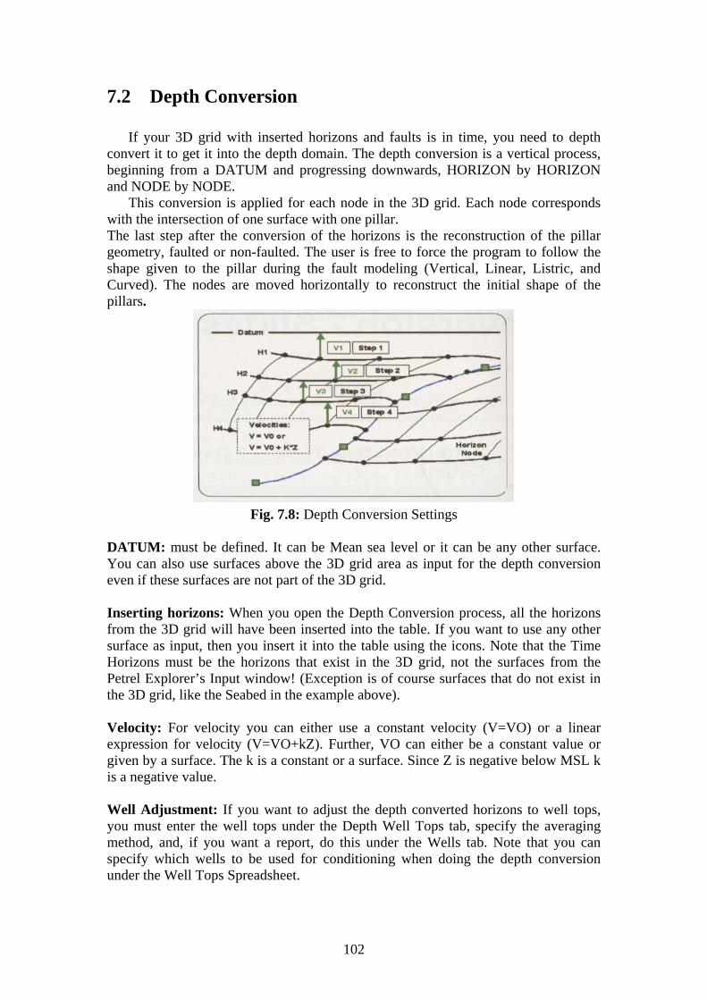
This conversion is applied for each node in the 3D grid. Each node corresponds with the intersection of one surface with one pillar. The last step after the conversion of the horizons is the reconstruction of the pillar geometry, faulted or non-faulted. The user is free to force the program to follow the shape given to the pillar during the fault modeling (Vertical, Linear, Listric, and Curved). The nodes are moved horizontally to reconstruct the initial shape of the pillars.

Fig. 7.8: Depth Conversion Settings DATUM: must be defined. It can be Mean sea level or it can be any other surface. You can also use surfaces above the 3D grid area as input for the depth conversion even if these surfaces are not part of the 3D grid. Inserting horizons: When you open the Depth Conversion process, all the horizons from the 3D grid will have been inserted into the table. If you want to use any other surface as input, then you insert it into the table using the icons. Note that the Time Horizons must be the horizons that exist in the 3D grid, not the surfaces from the Petrel Explorer’s Input window! (Exception is of course surfaces that do not exist in the 3D grid, like the Seabed in the example above). Velocity: For velocity you can either use a constant velocity (V=VO) or a linear expression for velocity (V=VO+kZ). Further, VO can either be a constant value or given by a surface. The k is a constant or a surface. Since Z is negative below MSL k is a negative value. Well Adjustment: If you want to adjust the depth converted horizons to well tops, you must enter the well tops under the Depth Well Tops tab, specify the averaging method, and, if you want a report, do this under the Wells tab. Note that you can specify which wells to be used for conditioning when doing the depth conversion under the Well Tops Spreadsheet.

102

7.3 Make Zones

The Make Zones process is the next step in defining the vertical resolution of the 3D grid. The process creates zones between each horizon. Zones can be added to the model by introducing thickness data in the form of isochores, constant thickness and percentages. Well points can also be used to tie top structures to the well picks. This process step may be skipped when no zonation is given.

To create zones follow the steps:

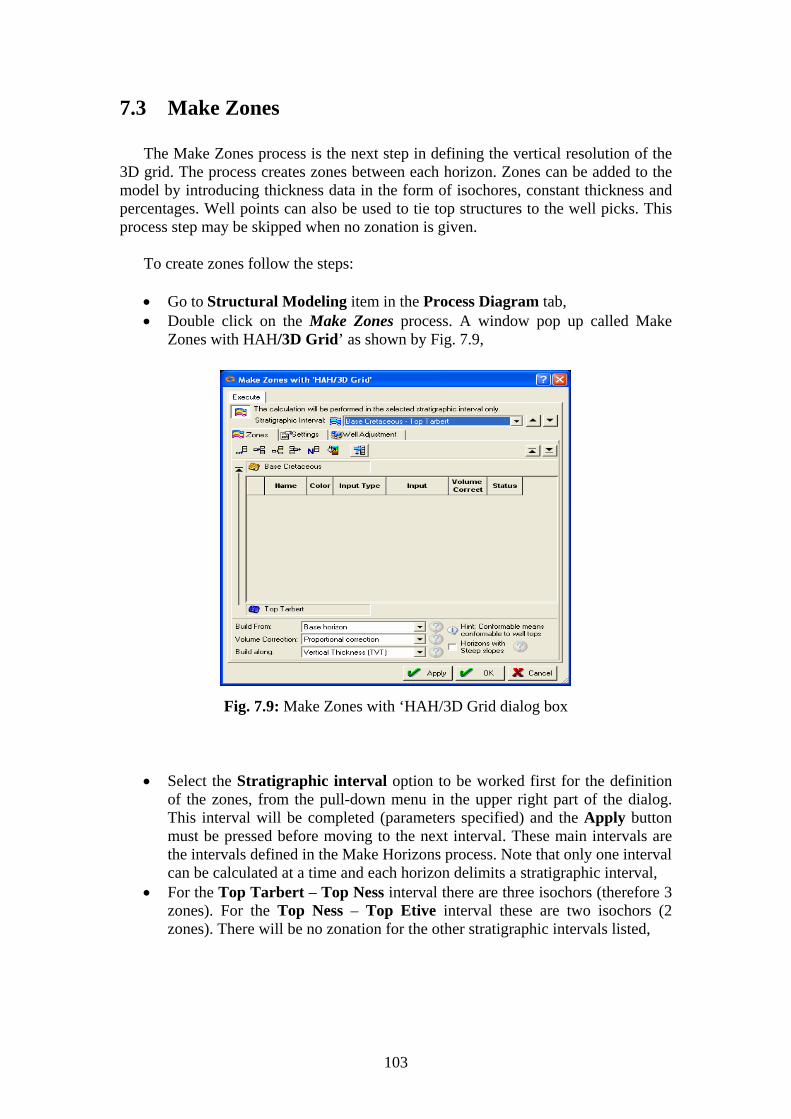
• Go to Structural Modeling item in the Process Diagram tab, • Double click on the Make Zones process. A window pop up called Make

Zones with HAH/3D Grid’ as shown by Fig. 7.9,

Fig. 7.9: Make Zones with ‘HAH/3D Grid dialog box

• Select the Stratigraphic interval option to be worked first for the definition of the zones, from the pull-down menu in the upper right part of the dialog. This interval will be completed (parameters specified) and the Apply button must be pressed before moving to the next interval. These main intervals are the intervals defined in the Make Horizons process. Note that only one interval can be calculated at a time and each horizon delimits a stratigraphic interval,

• For the Top Tarbert – Top Ness interval there are three isochors (therefore 3 zones). For the Top Ness – Top Etive interval these are two isochors (2 zones). There will be no zonation for the other stratigraphic intervals listed,

103

• Click on the Set number of items in table button and specify how many

zones you want in the current stratigraphic interval, or you can click on Append item in the table icon, as shown by Fig. 7.10,

• in this case insert 6 zones note that one click inserts three rows with two zone icons and one horizon icon (if the chosen stratigraphic interval are either Top – Mid or Mid – Base). The zone icons represent the isochores used for calculating the new intermediate horizon,

Fig. 7 hile Append item in the table and Set

number of items in the table appears .10: Make Zones with HAH/3D Grid w

• Insert the Isochores from the Isochores folder and the subfolder that

• ut field called

corresponds with the stratigraphic interval you are working on, Insert isochores by clicking on the blue arrow next to the inpInput, as shown by Fig. 7.11,

104

Fig. 7.11: Isochores placed in input

• Insert well tops between the isochores by going to Well Tops> Sorted on Type

and select the Well Tops that correspond with the Stratigraphic interval you working on,

• Select Build from base horizon and distribute the volume correction Proportionally among the various sub intervals,

• Select Build along Vertical Thickness (TVT), • Don't forget to repeat procedure for the other Stratigraphic interval, • Go to Setting tab and de-select the option that says:’ According to the setting

in the “Making Horizons” process as shown by Fig. 7.12,

Fig. 7.12: Make Zones with HAH/3D Grid dialog box

105

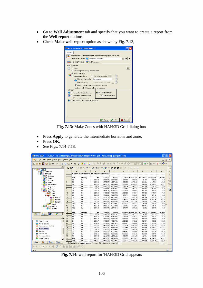
• Go to Well Adjustment tab and specify that you want to create a report from

the Well report options, • Check Make well report option as shown by Fig. 7.13,

Fig. 7.13: Make Zones with HAH/3D Grid dialog box

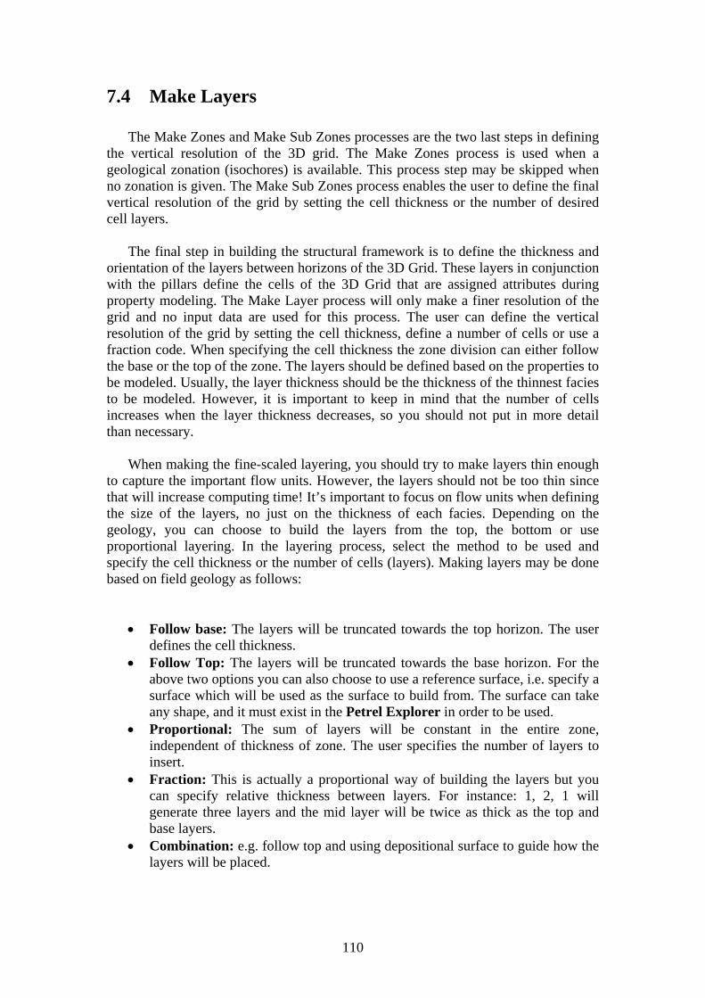
• Press Apply to generate the intermediate horizons and zone, • Press OK, • See Figs. 7.14-7.18.

Fig. 7.14: well report for 'HAH/3D Grid' appears

106

Fig. 7.15: Zones created in a 3D window while Pillar Gridding appears

Fig. 7.16: Zones created in 3D window along with their wells and faults

107

Fig. 7.17: Zones displayed while zones under Zones Filter created

Fig. 7.18: Zones displayed in a 3D window while Intersections are displayed

108

Noti

The colors of the zones can be changed from the Setting menu for each zone, found under the Zones filter in the bottom of the 3D Grid (DC).

7.3.1 Quality Control (QC) Using Intersection Planes

In order to move an intersection it must first be active (bold) in the Petrel Explorer. All intersections can be displayed in the Display window at the same time but only one can be moved at a time. More intersections in either direction can be inserted from the pull-down menu of the Intersection folder or from the Function bar. Playing trough the intersections in the main directions, I- and J-direction, are a good method to QC the 3D grid. The intersections will show how the pillars in the grid are situated next to each other. The 3D grid will get a vertical layering and definition when horizons are inserted in the next process step, but since the vertical definition will not change the pillars in the grid, a QC with intersections can also be done after this step. When quality controlling the 3D grid, it is important to look for neighboring pillars that have very different angles. This can introduce errors when inserting horizons and zones to the grid. Intersections in the I- or J-direction are created when generating the grid. They can be viewed in the Display window by opening the Intersection folder and selecting one or both of them. A new set of icons will be visible on the Status bar in the bottom of the Petrel window. For details on how to use the intersections, see How to use the I and J intersections.

ce:

109

7.4 Make Layers

eological zonation (isochores) is available. This process step may be skipped when o zonation is given. The Make Sub Zones process enables the user to define the final ertical resolution of the grid by setting the cell thickness or the number of desired ell layers.

The final step in building the structural framework is to define the thickness and rientation of the layers between horizons of the 3D Grid. These layers in conjunction ith the pillars define the cells of the 3D Grid that are assigned attributes during

odeling. The Make Layer process will only make a finer resolution of the rid and no input da a are used for this process. The user can define the vertical solution of the grid by setting the cell thickness, define a number of cells or use a action code. When specifying the cell thickness the zone division can either follow e base or the top of the zone. The layers should be defined based on the properties to

e modeled. Usually, the layer thickness should be the thickness of the thinnest facies be modeled. However, it is important to keep in mind that the number of cells creases when the layer thickness decreases, so you should not put in more detail an necessary.

layers thin enough c

es the number of layers to insert.

• Fraction: This is actually a proportional way of building the layers but you can specify relative thickness between layers. For instance: 1, 2, 1 will generate three layers and the mid layer will be twice as thick as the top and base layers.

• Combination: e.g. follow top and using depositional surface to guide how the layers will be placed.

The Make Zones and Make Sub Zones processes are the two last steps in defining

e vertical resolution of the 3D grid. The Make Zones process is used when a thgnvc

owproperty mg trefrthbtointh

When making the fine-scaled layering, you should try to make to apture the important flow units. However, the layers should not be too thin since that will increase computing time! It’s important to focus on flow units when defining the size of the layers, no just on the thickness of each facies. Depending on the geology, you can choose to build the layers from the top, the bottom or use proportional layering. In the layering process, select the method to be used and specify the cell thickness or the number of cells (layers). Making layers may be done based on field geology as follows:

• Follow base: The layers will be truncated towards the top horizon. The user defines the cell thickness.

• Follow Top: The layers will be truncated towards the base horizon. For the above two options you can also choose to use a reference surface, i.e. specify a surface which will be used as the surface to build from. The surface can take any shape, and it must exist in the Petrel Explorer in order to be used.

• Proportional: The sum of layers will be constant in the entire zone, independent of thickness of zone. The user specifi

110

To create layers follow t

he steps:

• Make sure you have one or both of the I and J intersections displayed in the

• g of the zones by clicking OK, and observe the

• •

ns,

• Go to Structural Modeling item in the Process Diagram tab, • Double click on the Layering process. A window pop up called Layering

with ‘HAH/3D Grid’ as shown by Fig. 7.19, this dialog has only one tab. In principle it works the same way as the Make Horizon and Make Zones dialogs - a spreadsheet with the zones as rows and the specific zone settings as columns,

Fig 7.19: Layering with ‘HAH/3D Grid dialog box

• The dialog lists the zones generated in the Make Horizons and Make Zones processes. For each zone select the desired resolution and layering layout.

graphics. Zoom in to see the full vertical interval. Create the internal layerinresults, Change the option under the Zone Division as shown in Fig. 7.20, The Horizons, Zones and Layering can be removed by clicking with the right mouse button on the 3D grid icon and selecting one of the Remove optio

• See Fig. 7.21, 7.22.

111

Fig. 7.20: Changing the setting on Layering with HAH/3D Grid’ dialog box

Fig. 7.21: Layers created in a 3D window while Layering with’HAH/3D Grid' appears

112

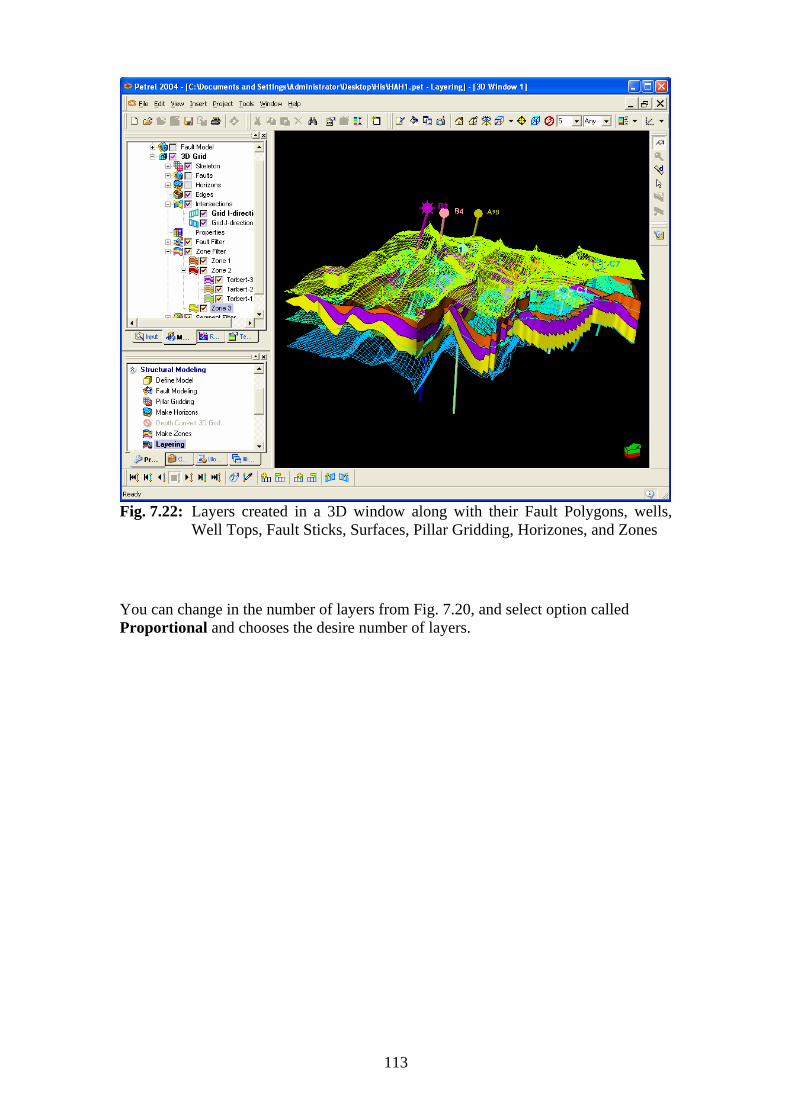
Fig. 7.22: Layers created in a 3D window along with their Fault Polygons, wells, Well Tops, Fault Sticks, Surfaces, Pillar Gridding, Horizones, and Zones

You can change in the number of layers from Fig. 7.20, and select option called Proportional and chooses the desire number of layers.

113