6 HANDWRITTEN CHARACTER RECOGNITION USING … CHARACT… · handwriting recognition systems ......
21
International Journal of Computer Engineering and Technology (IJCET), ISSN 0976-6367(Print), ISSN 0976 - 6375(Online), Volume 6, Issue 2, February (2015), pp. 54-74 © IAEME 54 HANDWRITTEN CHARACTER RECOGNITION USING FEED-FORWARD NEURAL NETWORK MODELS Nilay Karade 1 , Dr. Manu Pratap Singh 2 , Dr. Pradeep K. Butey 3 1 A-304, Shivpriya Towers, Jaitala, Nagpur-440039, Maharshatra, India 2 Department of Computer Science, Dr. B.R.Ambedkar University, Khandari, Agra - 282002, Uttar Pradesh, India 3 HOD (Computer Science), Kamala Nehru Mahavidyalaya, Nagpur, India ABSTRACT Handwritten character recognition has been vigorous and tough task in the field of pattern recognition. Considering its application to various fields, a lot of work is done and is being continuing to improve the results through various methods. In this paper we have proposed a system for individual handwritten character recognition using multilayer feed-forward neural networks. For the experimental purpose we have taken 15 samples of lower & upper case handwritten English alphabets in scanned image format i.e. 780 different handwritten character samples. There are two methods of feature extraction are used to construct the pattern vectors for training set. This training set is presented to the six different feed-forward neural networks namely newff, newfit, newpr, newgrnn, newrb and newrbe. The test pattern set is used to evaluate the performance of these neural networks models. The results are compared to find the accuracy in recognition of the respective models. The number of hidden layer, number of neurons in hidden layer, validation checks and gradient factors of the neural networks models are taken into consideration during the training. Keywords: Character Recognition, multilayer feed-forward Artificial Neural Network, Backpropagation, Handwriting recognition, Pattern Classification 1. INTRODUCTION These days computer have been penetrated in every field and the work is being done at a higher speed with greater accuracy. Pattern recognition through computer is a challenging task and this task becomes more critical if the pattern is in the form of handwritten curve script. Pattern INTERNATIONAL JOURNAL OF COMPUTER ENGINEERING & TECHNOLOGY (IJCET) ISSN 0976 – 6367(Print) ISSN 0976 – 6375(Online) Volume 6, Issue 2, February (2015), pp. 54-74 © IAEME: www.iaeme.com/IJCET.asp Journal Impact Factor (2015): 8.9958 (Calculated by GISI) www.jifactor.com IJCET © I A E M E
Transcript of 6 HANDWRITTEN CHARACTER RECOGNITION USING … CHARACT… · handwriting recognition systems ......
International Journal of Computer Engineering and Technology (IJCET), ISSN 0976-6367(Print),
ISSN 0976 - 6375(Online), Volume 6, Issue 2, February (2015), pp. 54-74 © IAEME
54
HANDWRITTEN CHARACTER RECOGNITION USING
FEED-FORWARD NEURAL NETWORK MODELS
Nilay Karade1, Dr. Manu Pratap Singh
2, Dr. Pradeep K. Butey
3
1A-304, Shivpriya Towers, Jaitala, Nagpur-440039, Maharshatra, India
2Department of Computer Science, Dr. B.R.Ambedkar University, Khandari,
Agra - 282002, Uttar Pradesh, India
3HOD (Computer Science), Kamala Nehru Mahavidyalaya, Nagpur, India
ABSTRACT
Handwritten character recognition has been vigorous and tough task in the field of pattern
recognition. Considering its application to various fields, a lot of work is done and is being
continuing to improve the results through various methods. In this paper we have proposed a system
for individual handwritten character recognition using multilayer feed-forward neural networks. For
the experimental purpose we have taken 15 samples of lower & upper case handwritten English
alphabets in scanned image format i.e. 780 different handwritten character samples. There are two
methods of feature extraction are used to construct the pattern vectors for training set. This training
set is presented to the six different feed-forward neural networks namely newff, newfit, newpr,
newgrnn, newrb and newrbe. The test pattern set is used to evaluate the performance of these neural
networks models. The results are compared to find the accuracy in recognition of the respective
models. The number of hidden layer, number of neurons in hidden layer, validation checks and
gradient factors of the neural networks models are taken into consideration during the training.
Keywords: Character Recognition, multilayer feed-forward Artificial Neural Network,
Backpropagation, Handwriting recognition, Pattern Classification
1. INTRODUCTION
These days computer have been penetrated in every field and the work is being done at a
higher speed with greater accuracy. Pattern recognition through computer is a challenging task and
this task becomes more critical if the pattern is in the form of handwritten curve script. Pattern
INTERNATIONAL JOURNAL OF COMPUTER ENGINEERING &
TECHNOLOGY (IJCET)
ISSN 0976 – 6367(Print)
ISSN 0976 – 6375(Online)
Volume 6, Issue 2, February (2015), pp. 54-74
© IAEME: www.iaeme.com/IJCET.asp
Journal Impact Factor (2015): 8.9958 (Calculated by GISI)
www.jifactor.com
IJCET
© I A E M E
International Journal of Computer Engineering and Technology (IJCET), ISSN 0976-6367(Print),
ISSN 0976 - 6375(Online), Volume 6, Issue 2, February (2015), pp. 54-74 © IAEME
55
recognition, as a subject, spans a number of scientific disciplines, uniting them in search for a
solution to the common problem of recognizing the pattern of a given class and assigning the name
of identified class. Pattern recognition is the categorization of input data into identifiable classes
through the extraction of significant attributes of the data from irrelevant background detail. A
pattern class is a category determined by some common attributes. It is true that the older
handwritten documents are digitized but the 100% automation of work cannot be achieved. The
handwriting recognition has helped a lot to the advancement of automation process [1]. The
handwriting recognition systems are broadly classified into two types, namely online and offline
handwritten recognition. In online approach, the two dimensional coordinates of the consecutive
points are symbolize as a function of time. Also the sequence of the strokes made by the writer is on
hand. Whereas in the case of off-line handwriting recognition approach the written script is captured
with the help of devices like scanner and the whole script is available as an image [2]. When both
these approaches are compared, it has been found that due the temporal information available with
the online approach, it is superior to that of off line approach [3]. On the other hand in the off-line
systems, the neural networks have been productively used for capitulate comparably high recognition
accuracy levels [1]. A number of applications such as document analysis, mailing address
interpretation, bank processing etc. require offline handwriting recognition system [1, 4]. Thus, the
off-line handwriting recognition enjoys the first choice by many researchers in order to investigate
and discover the novel methods that would get better recognition correctness. It is widely used in
image processing, pattern recognition, and artificial intelligence.
During the last few years the researchers have proposed many mathematical approaches to
solve the pattern recognition problems. Recognition strategies heavily depend on the nature of the
data to be recognized. In the cursive case, the problem is made complex by the fact that the writing is
fundamentally ambiguous as the letters in the word are generally linked together, poorly written and
may even be missing. On the contrary, hand printed word recognition is more related to printed word
recognition, the individual letters composing the word being usually much easier to isolate and to
identify. As a consequence of this, methods working on a letter basis (i.e., based on character
segmentation and recognition) are well suited to hand printed word recognition while cursive scripts
require more specific and/or sophisticated techniques. Inherent ambiguity must then be compensated
by the use of contextual information.
Neural network computing has been expected to play a significant role in a computer-based
system of recognizing handwritten characters. This is because a neural network can be trained quite
readily to recognize several instances of a written letter or word, and can then be generalized to
recognize other different instances of that same letter or word. This capability is vital to the
realization of robust recognition of handwritten characters or scripts, since characters are rarely
written twice in exactly the same form. There have been reports of successful use of neural networks
for the recognition of handwritten characters [11, 12], but we are not aware of any general
investigation which might shed light on the systematic approach of a complete neural network
system for the automatic recognition of cursive character. The techniques of artificial neural
networks are widely used for pattern recognition task over the conventional approaches to handle
such type of problem due to the following reasons:
1. The same alphabet character written by the same person can vary in shape, size and style.
2. It is not only the case with same person but also the shape, size and style of the same character
can vary from person to person.
3. Character image scanned in offline method might have poor quality due to noise present within
it.
4. As there are no pre defined rules about the look of the visual character, the rules should be
heuristically deduced form the set of sample data. The human brain by its very nature does the
same thing using the features discussed in the following two points.
International Journal of Computer Engineering and Technology (IJCET), ISSN 0976-6367(Print),
ISSN 0976 - 6375(Online), Volume 6, Issue 2, February (2015), pp. 54-74 © IAEME
56
5. The human brain can read handwritings of various people having different fashion of writing
because it is adaptive to slight variations and errors in pattern.
6. It can take hold of new styles present in the character due to its ability of learning from
experiences with no time.
J. Praddep, E.Srinivasan,and S.Himavathi [1] have proposed a handwritten character
recognition system using neural network by means of diagonal based feature extraction method.
They have stated with the binarization of the image which results in binary image, which further
undergoes the edge detection and dilation and then segmentation. In the process of segmentation a
series of characters is decomposed into sub image of each individual character, each of which is
converted into 90x60 pixels for classification and recognition process. Each character image
obtained in such a way that it is divided into 54 equal zones, each of size 10 x10 pixels and
then features are extracted from each zone pixels by moving along its diagonals. They have
ended up with 54 features for each of the character. Another feature extraction method gives them 69
features by averaging the values placed in zones row wise and column wise. A feed forward back
propagation neural network having two hidden layers with architecture of 54-100-100-38 is used to
perform the classification with both the features with vertical, horizontal and diagonal orientation
and have found 92.69, 93.68 , 97.80 percent accuracy and 92.69, 94.73, 98.54 percent accuracy,
respectively.
Kauleshwar Prasad, Devvrat C. Nigam, Ashmika Lakhotiya and Dheeren Umre [3] have
converted the character image into a binary image, and then apply character extraction algorithm in
which it has empty traverse list initially. A row is scan pixel by pixel and on getting black pixel, it is
checked if it is already in the traverse list. It is checked that if it is already there then it is ignored,
otherwise added to the traverse list using edge detection algorithm. They have claimed to have good
results by using feed-forward Backpropagation neural network and also stated that poorly chosen
feature extraction method gives poor results.
Ankit Sharma and Dipti R Chaudhary [4] have achieved the accuracy of 85%, using feed
forward neural network. The special form of Reduction is used which includes the noise removal and
edge detection for the feature extraction of grayscale images.
Chirag I Patel, Ripal Patel, Palak Patel [5] have achieved the accuracy of 91%, 889%, 91%,
91%, 94%, 94% using different models of Backpropagation neural networks. After character
extraction and edge detection from the document, it goes under the process of normalization where
the images having various sizes are normalized to a uniform size. The resultant image is applied with
‘Line Fitting’, a skew detection technique to correct this skewedness, in which it is rotated by an
angle θ. The constructed pattern from this method is further used for the training by Backpropagation
algorithm of feed-forward multilayer neural networks.
Anita Pal and Dayashankar [7] have used a multilayer perceptron with one hidden layer to
recognize Handwritten English Character. Boundary tracing along with Fourier Descriptor is used to
extract the feature from the handwritten character. By analyzing its shape and judge against its
features, a character is identified. Test result was found to have fine recognition accuracy of 94%
for handwritten English characters with less training time.
The genetic algorithm is used with feed forward neural network architecture as the hybrid
evolutionary algorithm [27] for the recognition of handwritten English alphabets. In this paper each
character is considered as the gray level image and divided into sixteen parts. The mean of each part
is considered as one feature of the pattern. Thus, there are sixteen features in real numbers are used
as the pattern vector for each image. The trained network performed well for the pattern
classification for test patterns.
In this paper we consider the two approaches of feature extraction from the images of
handwritten capital and small letters of English alphabets. The first method of feature extraction uses
the row wise mean value of the pixels for a processed image of size n x n. The second method
International Journal of Computer Engineering and Technology (IJCET), ISSN 0976-6367(Print),
ISSN 0976 - 6375(Online), Volume 6, Issue 2, February (2015), pp. 54-74 © IAEME
57
consider the each pixel value of the dilated image of size n x n. These features are used to construct
the pattern vectors. The two training sets are formed from these samples examples of pattern vectors.
There are six different feed forward neural networks models are used with six different learning
methods. The performances of these neural networks with different learning rules are analyzed. The
rate of recognition for patterns from the test pattern set is also evaluated. The performance evaluation
indicates that the Radial bias function (RBF) neural network architecture performs better than other
neural network models for both the methods of feature extraction. The rate of recognition for test
pattern set in RBF is found better with respect to other neural network models.
Rest of the paper is containing 6 sections. Section 2 of the paper describes the feature
extraction methods for handwritten English characters. The section 3 discusses about feed forward
neural networks and Backpropagation learning and Radial basis function. The section 4 describes the
experiment and simulation design. The Section 5 presents the simulated results and discussion.
Section 6 describes the conclusion followed by the references.
2. FEATURE EXTRACTION
Feature extraction and selection can be defined as extracting the most representative
information from the raw data, which minimizes within class. The pattern variability while
enhancing between class pattern variability so that, a set of feature are extracted from each class that
helps to distinguish it from other classes, while remaining invariant to characteristic differences
within the class. Here we are considering the feature extraction from the input stimuli with two
methods namely the row wise mean of pixel from a scanned image and each pixel value of the
image. In our approaches we have considered the input data in the form of fifteen different set of
each hand written capital and small English characters by five different peoples. It is quite natural
that the five different people considered the different hand writing and different writing style for
every character. So, in this way we have total 780 samples. Among these 780 samples we used 520
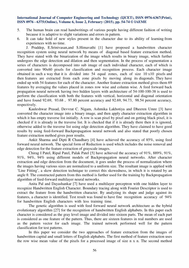
samples for training and the remaining 260 samples were used in test pattern set. Now to prepare our
training set of input output pattern pairs, we consider each scanned hand written character as a color
bit map image. This color bitmap image of a character is now changed into gray level image and then
into binary image as shown in figure 1.
Fig 1 (a) gray level image Fig 1 (b) Binary Image
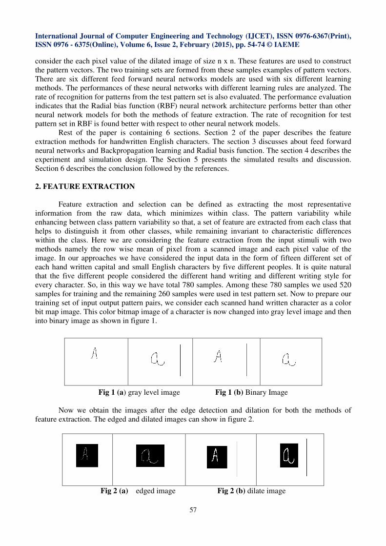
Now we obtain the images after the edge detection and dilation for both the methods of
feature extraction. The edged and dilated images can show in figure 2.
Fig 2 (a) edged image Fig 2 (b) dilate image
International Journal of Computer Engineering and Technology (IJCET), ISSN 0976-6367(Print),
ISSN 0976 - 6375(Online), Volume 6, Issue 2, February (2015), pp. 54-74 © IAEME
58
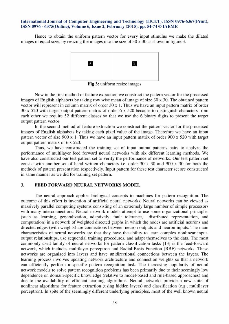
Hence to obtain the uniform pattern vector for every input stimulus we make the dilated
images of equal sizes by resizing the images into the size of 30 x 30 as shown in figure 3.
Fig 3: uniform resize images
Now in the first method of feature extraction we construct the pattern vector for the processed
images of English alphabets by taking row wise mean of image of size 30 x 30. The obtained pattern
vector will represent in column matrix of order 30 x 1. Thus we have an input pattern matrix of order
30 x 520 with target output pattern matrix of order 6 x 520 because to distinguish characters from
each other we require 52 different classes so that we use the 6 binary digits to present the target
output pattern vector.
In the second method of feature extraction we construct the pattern vector for the processed
images of English alphabets by taking each pixel value of the image. Therefore we have an input
pattern vector of size 900 x 1. Thus we have an input pattern matrix of order 900 x 520 with target
output pattern matrix of 6 x 520.
Thus, we have constructed the training set of input output patterns pairs to analyze the
performance of multilayer feed forward neural networks with six different learning methods. We
have also constructed our test pattern set to verify the performance of networks. Our test pattern set
consist with another set of hand written characters i.e. order 30 x 30 and 900 x 30 for both the
methods of pattern presentation respectively. Input pattern for these test character set are constructed
in same manner as we did for training set pattern.
3. FEED FORWARD NEURAL NETWORKS MODEL
The neural approach applies biological concepts to machines for pattern recognition. The
outcome of this effort is invention of artificial neural networks. Neural networks can be viewed as
massively parallel computing systems consisting of an extremely large number of simple processors
with many interconnections. Neural network models attempt to use some organizational principles
(such as learning, generalization, adaptively, fault tolerance, distributed representation, and
computation) in a network of weighted directed graphs in which the nodes are artificial neurons and
directed edges (with weights) are connections between neuron outputs and neuron inputs. The main
characteristics of neural networks are that they have the ability to learn complex nonlinear input-
output relationships, use sequential training procedures, and adapt themselves to the data. The most
commonly used family of neural networks for pattern classification tasks [13] is the feed-forward
network, which includes multilayer perceptron and Radial-Basis Function (RBF) networks. These
networks are organized into layers and have unidirectional connections between the layers. The
learning process involves updating network architecture and connection weights so that a network
can efficiently perform a specific pattern recognition task. The increasing popularity of neural
network models to solve pattern recognition problems has been primarily due to their seemingly low
dependence on domain-specific knowledge (relative to model-based and rule-based approaches) and
due to the availability of efficient learning algorithms. Neural networks provide a new suite of
nonlinear algorithms for feature extraction (using hidden layers) and classification (e.g., multilayer
perceptron). In spite of the seemingly different underlying principles, most of the well known neural
International Journal of Computer Engineering and Technology (IJCET), ISSN 0976-6367(Print),
ISSN 0976 - 6375(Online), Volume 6, Issue 2, February (2015), pp. 54-74 © IAEME
59
network models are implicitly equivalent or similar to classical statistical pattern recognition
methods. Ripley [14] and Anderson et al. [15] also discuss the relationship between neural networks
and statistical pattern recognition. Despite these similarities, neural networks do offer several
advantages such as, unified approaches for feature extraction & classification and flexible procedures
for finding good, moderately nonlinear solutions. The advantages of neural networks are their
adaptive-learning, self-organization and fault-tolerance capabilities. For these outstanding
capabilities, neural networks are used for pattern recognition applications. The goal in pattern
recognition is to use a set of example solutions to some problem to infer an underlying regularity
which can subsequently be used to solve new instances of the problem. In the case of feed-forward
networks, the set of example solutions (called a training set), comprises sets of input values together
with corresponding sets of desired output values. The training set is used to determine an error
function in terms of the discrepancy between the predictions of the network, for given inputs, and the
desired values of the outputs given by the training set. A common example of an error function
would be the squared difference between desired and actual output, summed over all outputs and
summed over all patterns in the training set. The learning process then involves adjusting the values
of the parameters to minimize the value of the error function. This kind of error Backpropagation
would be used to reconstruct the input patterns and make them free from error which increases the
performance of the neural networks. However, effective learning algorithms were only known for the
case of networks in which at most one of the layers comprised adaptive interconnections. Such
networks were known variously as perceptron [16] and Adaline [17], and were seriously limited in
their capabilities [18].
The feed forward neural network consists of an input layer of units, one or more hidden
layers, and an output layer. Each node in the layer has one corresponding node in the next layer,
thus creating the stacking effect. The input layer’s nodes have output functions that deliver data to
the first hidden layer nodes. The hidden layer(s) are the processing layer, where all of the actual
computation takes place. Each node in hidden layer computes a sum based on its input from the
previous layer (either the input layer or another hidden layer). The sum is then “compacted” by a
sigmoid function (a logistic transfer function), which changes the sum to a limited and manageable
range. The output sum from the hidden layers is passed on to the output layer, which produces the
final network. The feed-forward networks may contain any number of hidden layers, network with
a single hidden layer can learn any set of training data that a network with multiple layers can
learn, depends upon the complexity of the problem [19]. In feed forward neural network an input
may be either a raw/preprocessed signal or image. Alternatively, some specific features can also be
used. If specific features are used as input, there number and selection is crucial and application
dependent. Weights are connected between an input and a summing node and affect to the
summing operation. The Bias or threshold value is considered as a weight with constant input 1 i.e.
x0=1 and w0=θ, usually the weight are randomized in the beginning [20, 21].
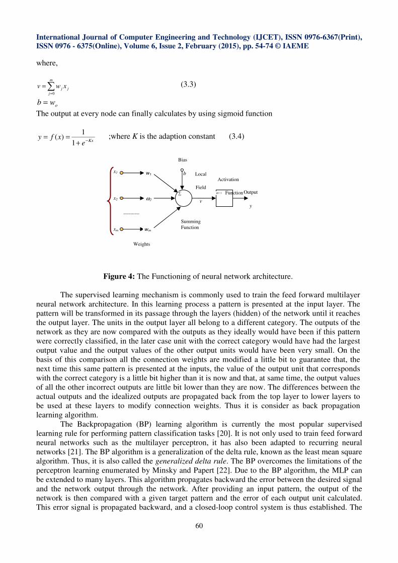
The neuron is the basic information processing unit of a neural network. It consists of: A set of
links, describing the neuron inputs, with weights, w1,w2,w3….wn , An adder function (linear
combiner) for computing the weighted sum as:
j
m
j
j xwv ∑=
=1
(3.1)
And activation function (squashing function) for limiting the amplitude of the neuron output as
shown in figure 3.1
)( bvy += ϕ (3.2)
International Journal of Computer Engineering and Technology (IJCET), ISSN 0976-6367(Print),
ISSN 0976 - 6375(Online), Volume 6, Issue 2, February (2015), pp. 54-74 © IAEME
60
where,
j
m
j
j xwv ∑=
=0
(3.3)
owb =
The output at every node can finally calculates by using sigmoid function
Kxexfy
−+==
1
1)( ;where K is the adaption constant (3.4)
Figure 4: The Functioning of neural network architecture.
The supervised learning mechanism is commonly used to train the feed forward multilayer
neural network architecture. In this learning process a pattern is presented at the input layer. The
pattern will be transformed in its passage through the layers (hidden) of the network until it reaches
the output layer. The units in the output layer all belong to a different category. The outputs of the
network as they are now compared with the outputs as they ideally would have been if this pattern
were correctly classified, in the later case unit with the correct category would have had the largest
output value and the output values of the other output units would have been very small. On the
basis of this comparison all the connection weights are modified a little bit to guarantee that, the
next time this same pattern is presented at the inputs, the value of the output unit that corresponds
with the correct category is a little bit higher than it is now and that, at same time, the output values
of all the other incorrect outputs are little bit lower than they are now. The differences between the
actual outputs and the idealized outputs are propagated back from the top layer to lower layers to
be used at these layers to modify connection weights. Thus it is consider as back propagation
learning algorithm.
The Backpropagation (BP) learning algorithm is currently the most popular supervised
learning rule for performing pattern classification tasks [20]. It is not only used to train feed forward
neural networks such as the multilayer perceptron, it has also been adapted to recurring neural
networks [21]. The BP algorithm is a generalization of the delta rule, known as the least mean square
algorithm. Thus, it is also called the generalized delta rule. The BP overcomes the limitations of the
perceptron learning enumerated by Minsky and Papert [22]. Due to the BP algorithm, the MLP can
be extended to many layers. This algorithm propagates backward the error between the desired signal
and the network output through the network. After providing an input pattern, the output of the
network is then compared with a given target pattern and the error of each output unit calculated.
This error signal is propagated backward, and a closed-loop control system is thus established. The
Weights
Summing
Function
Bias
b
Activation
Function
Local
Field
v
Output
y
x1
x2
xm
ω2
wm
w1
∑ )(−ϕ
………….
International Journal of Computer Engineering and Technology (IJCET), ISSN 0976-6367(Print),
ISSN 0976 - 6375(Online), Volume 6, Issue 2, February (2015), pp. 54-74 © IAEME
61
weights can be adjusted by a gradient-descent approach. In order to implement the BP algorithm, a
continuous, nonlinear, monotonically increasing, differentiable activation function is required as
Logistic Sigmoid function or hyperbolic tangent function.
So that, to provide the training for multi-layer feed forward network to approximate an
unknown function, based on some training data consisting of pairs ( ) Szx ∈, , the input pattern vector
x represents a pattern of input to the network, with desired output pattern vector z from the training
set S. The objective function for optimization or minimization is defined in the sum of
instantaneously squared error as:
∑=
−=J
j
jj
P STE1
2)(2
1 (3.5)
where 2
)( jj ST − is the squared difference between the actual output of the network on the output
layer for the presented input pattern P and the target output pattern vector for the pattern P. All the
network parameters ( )1−mW and mθ , m = 2 ・ ・ ・M, can be combined and represented by the matrix
[ ]ijwW = . So that, the error function E can be minimized by applying the gradient-descent procedure
as:
W
EW
∂
∂−=∆ η (3.6)
where η is a learning rate or step size, provided that it is a sufficiently small positive number.
Applying the chain rule the equation (3.6) can express as
( ) ( )
( )
( )mij
mj
mj
mij w
u
u
E
w
E
∂
∂
∂
∂=
∂
∂ +
+
1
1 (3.7)
while ( )
( ) ( )( ) ( ) ( )( ) ( )m
im
jmm
jmij
mij
mj
oowww
u=+
∂
∂=
∂
∂∑
+
+
1
1
θ (3.8)
and ( ) ( )
( )
( ) ( )( ) ( )( )11
1
1
11
++
++
+
++ ∂
∂=
∂
∂
∂
∂=
∂
∂m
j
m
jm
j
im
j
m
j
m
j
m
j
uo
E
u
o
o
E
u
Eφ (3.9)
For the output unit m=M-1
( ) jmj
eo
E=
∂
∂+1
(3.10)
For the hidden units, m = 1,2,3………,M − 2,
( )
1
221
2
+
=++ ∑
+
∂
∂=
∂
∂ mj
j
mmj
m
u
E
o
Eω
ω ω
ω (3.11)
Define the delta function by
( )( )mp
mj
u
E
∂
∂=δ (3.12)
International Journal of Computer Engineering and Technology (IJCET), ISSN 0976-6367(Print),
ISSN 0976 - 6375(Online), Volume 6, Issue 2, February (2015), pp. 54-74 © IAEME
62
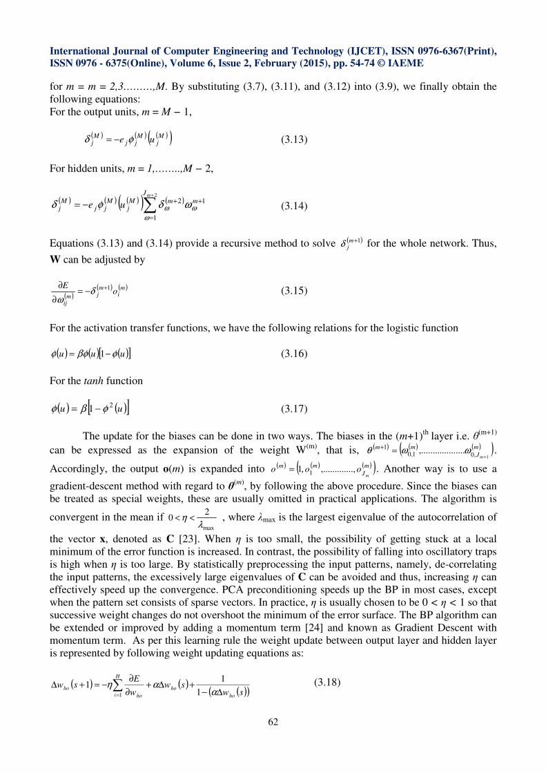
for m = m = 2,3………,M. By substituting (3.7), (3.11), and (3.12) into (3.9), we finally obtain the
following equations:
For the output units, m = M − 1,
( ) ( ) ( )( )M
jM
jjM
j ue φδ −= (3.13)
For hidden units, m = 1,……..,M − 2,
( ) ( ) ( )( ) ( ) 1
1
22
+
=
+∑
+
−= m
J
mMj
Mjj
Mj
m
ue ω
ω
ω ωδφδ (3.14)
Equations (3.13) and (3.14) provide a recursive method to solve ( )1+mjδ for the whole network. Thus,
W can be adjusted by
( )( ) ( )m
im
jmij
oE 1+−=
∂
∂δ
ω (3.15)
For the activation transfer functions, we have the following relations for the logistic function
( ) ( ) ( )[ ]uuu φβφφ −= 1 (3.16)
For the tanh function
( ) ( )[ ]uu21 φβφ −= (3.17)
The update for the biases can be done in two ways. The biases in the (m+1)th
layer i.e. θ(m+1)
can be expressed as the expansion of the weight W(m)
, that is, ( ) ( ) ( )( )m
J
mm
m 1,01,01 ..........,.........
+=+ ωωθ .
Accordingly, the output o(m) is expanded into ( ) ( ) ( )( )m
J
mm
mooo ....,,.........,1 1= . Another way is to use a
gradient-descent method with regard to θ(m)
, by following the above procedure. Since the biases can
be treated as special weights, these are usually omitted in practical applications. The algorithm is
convergent in the mean if max
20
λη << , where λmax is the largest eigenvalue of the autocorrelation of
the vector x, denoted as C [23]. When η is too small, the possibility of getting stuck at a local
minimum of the error function is increased. In contrast, the possibility of falling into oscillatory traps
is high when η is too large. By statistically preprocessing the input patterns, namely, de-correlating
the input patterns, the excessively large eigenvalues of C can be avoided and thus, increasing η can
effectively speed up the convergence. PCA preconditioning speeds up the BP in most cases, except
when the pattern set consists of sparse vectors. In practice, η is usually chosen to be 0 < η < 1 so that
successive weight changes do not overshoot the minimum of the error surface. The BP algorithm can
be extended or improved by adding a momentum term [24] and known as Gradient Descent with
momentum term. As per this learning rule the weight update between output layer and hidden layer
is represented by following weight updating equations as:
( ) ( )( )( )sw
sww
Esw
ho
H
i
ho
ho
ho∆−
+∆+∂
∂−=+∆ ∑
= ααη
1
11
1
(3.18)
International Journal of Computer Engineering and Technology (IJCET), ISSN 0976-6367(Print),
ISSN 0976 - 6375(Online), Volume 6, Issue 2, February (2015), pp. 54-74 © IAEME
63
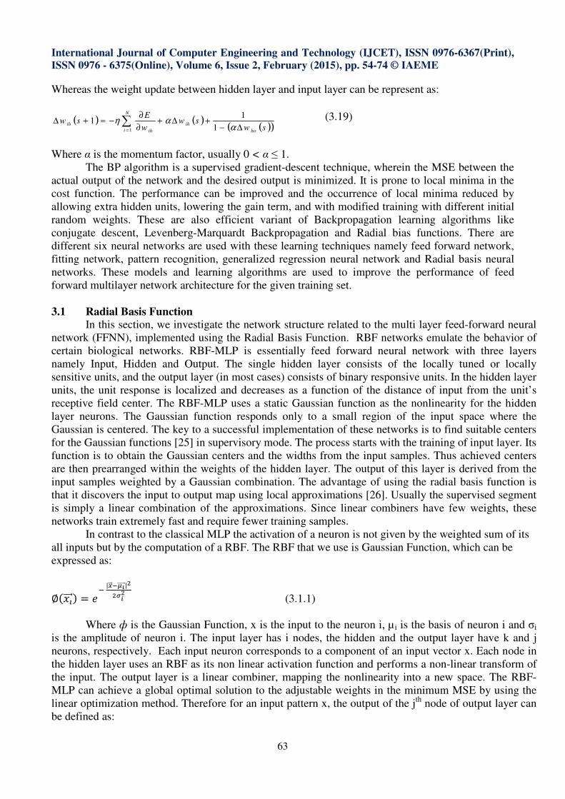
Whereas the weight update between hidden layer and input layer can be represent as:
( ) ( )( )( )sw
sww
Esw
ho
N
i
ih
ih
ih∆−
+∆+∂
∂−=+∆ ∑
= ααη
1
11
1
(3.19)
Where α is the momentum factor, usually 0 < α ≤ 1.
The BP algorithm is a supervised gradient-descent technique, wherein the MSE between the
actual output of the network and the desired output is minimized. It is prone to local minima in the
cost function. The performance can be improved and the occurrence of local minima reduced by
allowing extra hidden units, lowering the gain term, and with modified training with different initial
random weights. These are also efficient variant of Backpropagation learning algorithms like
conjugate descent, Levenberg-Marquardt Backpropagation and Radial bias functions. There are
different six neural networks are used with these learning techniques namely feed forward network,
fitting network, pattern recognition, generalized regression neural network and Radial basis neural
networks. These models and learning algorithms are used to improve the performance of feed
forward multilayer network architecture for the given training set.
3.1 Radial Basis Function
In this section, we investigate the network structure related to the multi layer feed-forward neural
network (FFNN), implemented using the Radial Basis Function. RBF networks emulate the behavior of
certain biological networks. RBF-MLP is essentially feed forward neural network with three layers
namely Input, Hidden and Output. The single hidden layer consists of the locally tuned or locally
sensitive units, and the output layer (in most cases) consists of binary responsive units. In the hidden layer
units, the unit response is localized and decreases as a function of the distance of input from the unit’s
receptive field center. The RBF-MLP uses a static Gaussian function as the nonlinearity for the hidden
layer neurons. The Gaussian function responds only to a small region of the input space where the
Gaussian is centered. The key to a successful implementation of these networks is to find suitable centers
for the Gaussian functions [25] in supervisory mode. The process starts with the training of input layer. Its
function is to obtain the Gaussian centers and the widths from the input samples. Thus achieved centers
are then prearranged within the weights of the hidden layer. The output of this layer is derived from the
input samples weighted by a Gaussian combination. The advantage of using the radial basis function is
that it discovers the input to output map using local approximations [26]. Usually the supervised segment
is simply a linear combination of the approximations. Since linear combiners have few weights, these
networks train extremely fast and require fewer training samples.
In contrast to the classical MLP the activation of a neuron is not given by the weighted sum of its
all inputs but by the computation of a RBF. The RBF that we use is Gaussian Function, which can be
expressed as:
∅�������� =
| �����������|�
����
(3.1.1)
Where ф is the Gaussian Function, x is the input to the neuron i, µ i is the basis of neuron i and σi
is the amplitude of neuron i. The input layer has i nodes, the hidden and the output layer have k and j
neurons, respectively. Each input neuron corresponds to a component of an input vector x. Each node in
the hidden layer uses an RBF as its non linear activation function and performs a non-linear transform of
the input. The output layer is a linear combiner, mapping the nonlinearity into a new space. The RBF-
MLP can achieve a global optimal solution to the adjustable weights in the minimum MSE by using the
linear optimization method. Therefore for an input pattern x, the output of the jth
node of output layer can
be defined as:
International Journal of Computer Engineering and Technology (IJCET), ISSN 0976-6367(Print),
ISSN 0976 - 6375(Online), Volume 6, Issue 2, February (2015), pp. 54-74 © IAEME
64
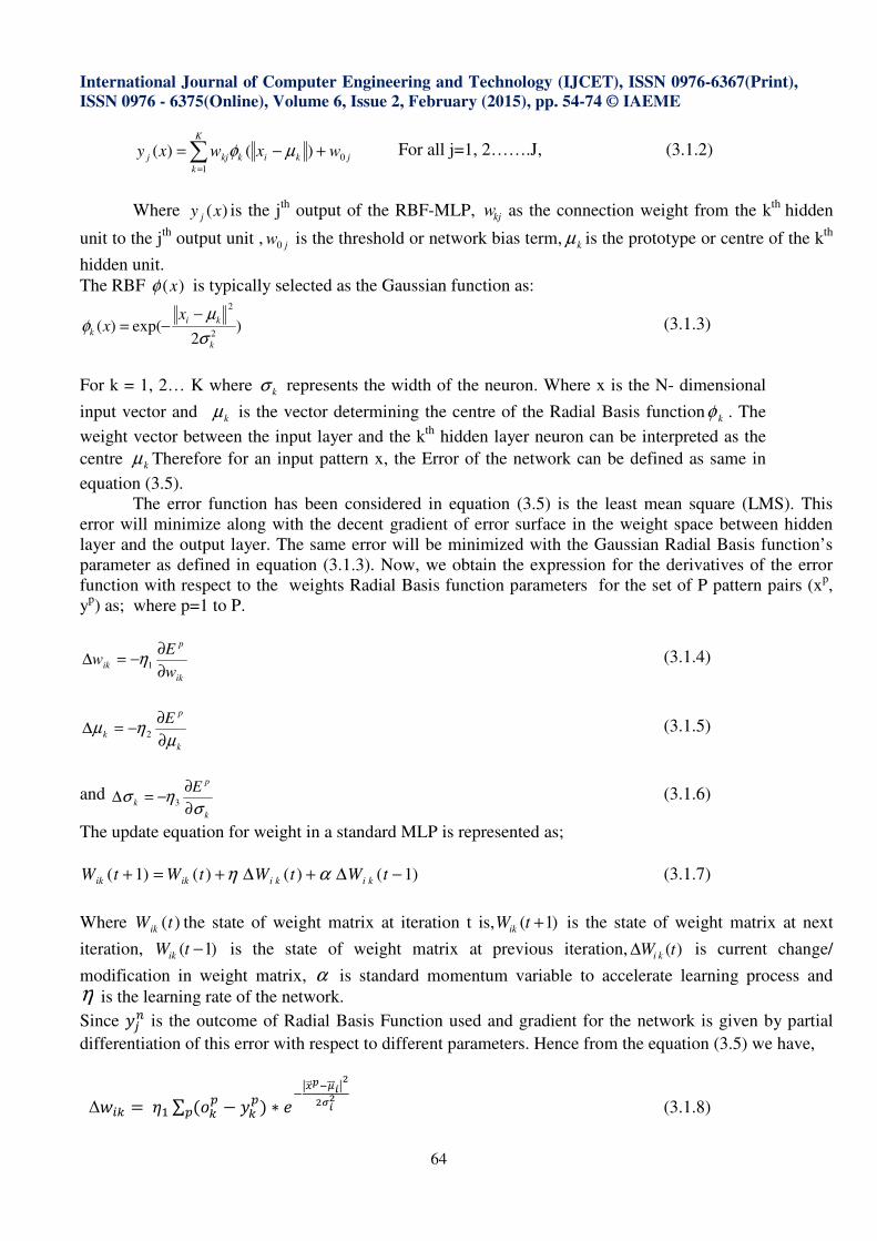
j
K
k
kikkjj wxwxy 0
1
)()( +−=∑=
µφ For all j=1, 2…….J, (3.1.2)
Where )(xy j is the jth
output of the RBF-MLP, kjw as the connection weight from the kth
hidden
unit to the jth
output unit , jw0 is the threshold or network bias term, kµ is the prototype or centre of the kth
hidden unit.
The RBF )(xφ is typically selected as the Gaussian function as:
)2
exp()(2
2
k
ki
k
xx
σ
µφ
−−= (3.1.3)
For k = 1, 2… K where kσ represents the width of the neuron. Where x is the N- dimensional
input vector and kµ is the vector determining the centre of the Radial Basis function kφ . The
weight vector between the input layer and the kth
hidden layer neuron can be interpreted as the
centre kµ Therefore for an input pattern x, the Error of the network can be defined as same in
equation (3.5).
The error function has been considered in equation (3.5) is the least mean square (LMS). This
error will minimize along with the decent gradient of error surface in the weight space between hidden
layer and the output layer. The same error will be minimized with the Gaussian Radial Basis function’s
parameter as defined in equation (3.1.3). Now, we obtain the expression for the derivatives of the error
function with respect to the weights Radial Basis function parameters for the set of P pattern pairs (xp,
yp) as; where p=1 to P.
ik
p
ikw
Ew
∂
∂−=∆ 1η (3.1.4)
k
p
k
E
µηµ
∂
∂−=∆ 2
(3.1.5)
and k
p
k
E
σησ
∂
∂−=∆ 3
(3.1.6)
The update equation for weight in a standard MLP is represented as;
)1()()()1( −∆+∆+=+ tWtWtWtW kikiikik αη (3.1.7)
Where )(tWik the state of weight matrix at iteration t is, )1( +tWik is the state of weight matrix at next
iteration, )1( −tWik is the state of weight matrix at previous iteration, )(tW ki∆ is current change/
modification in weight matrix, α is standard momentum variable to accelerate learning process and η is the learning rate of the network.
Since ��� is the outcome of Radial Basis Function used and gradient for the network is given by partial
differentiation of this error with respect to different parameters. Hence from the equation (3.5) we have,
∆��� =�� ∑ ���� − ��
��� ∗ ! ���"������!
�
����
(3.1.8)
International Journal of Computer Engineering and Technology (IJCET), ISSN 0976-6367(Print),
ISSN 0976 - 6375(Online), Volume 6, Issue 2, February (2015), pp. 54-74 © IAEME
65
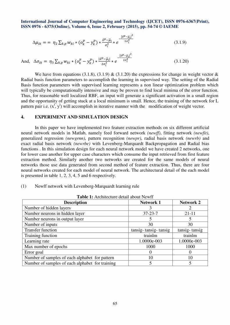
∆#�� == �$ ∑ ��� ∗ ���� − ��
���,� ∗ &�"'����(�� ∗
! ���"������!
�
����
(3.1.9)
And, ∆)�� =�* ∑ ��� ∗ ���� − ��
���,� ∗|&�"'����|
$(�+ ∗
! ���"������!
�
����
(3.1.20)
We have from equations (3.1.8), (3.1.9) & (3.1.20) the expressions for change in weight vector &
Radial basis function parameters to accomplish the learning in supervised way. The setting of the Radial
Basis function parameters with supervised learning represents a non linear optimization problem which
will typically be computationally intensive and may be proven to find local minima of the error function.
Thus, for reasonable well localized RBF, an input will generate a significant activation in a small region
and the opportunity of getting stuck at a local minimum is small. Hence, the training of the network for L
pattern pair i.e. (xl, y
l) will accomplish in iterative manner with the modification of weight vector.
4. EXPERIMENT AND SIMULATION DESIGN
In this paper we have implemented two feature extraction methods on six different artificial
neural network models in Matlab, namely feed forward network (newff), fitting network (newfit),
generalized regression (newgrnn), pattern recognition (newpr), radial basis network (newrb) and
exact radial basis network (newrbe) with Levenberg-Marquardt Backpropagation and Radial bias
functions . In this simulation design for each neural network model we have created 2 networks, one
for lower case another for upper case characters which consume the input retrieved from first feature
extraction method. Similarly another two networks are created for the same models of neural
networks those use data generated from second method of feature extraction. Thus, there are four
neural networks created for each model of neural network. The architectural detail of the each model
is presented in table 1, 2, 3, 4, 5 and 6 respectively.
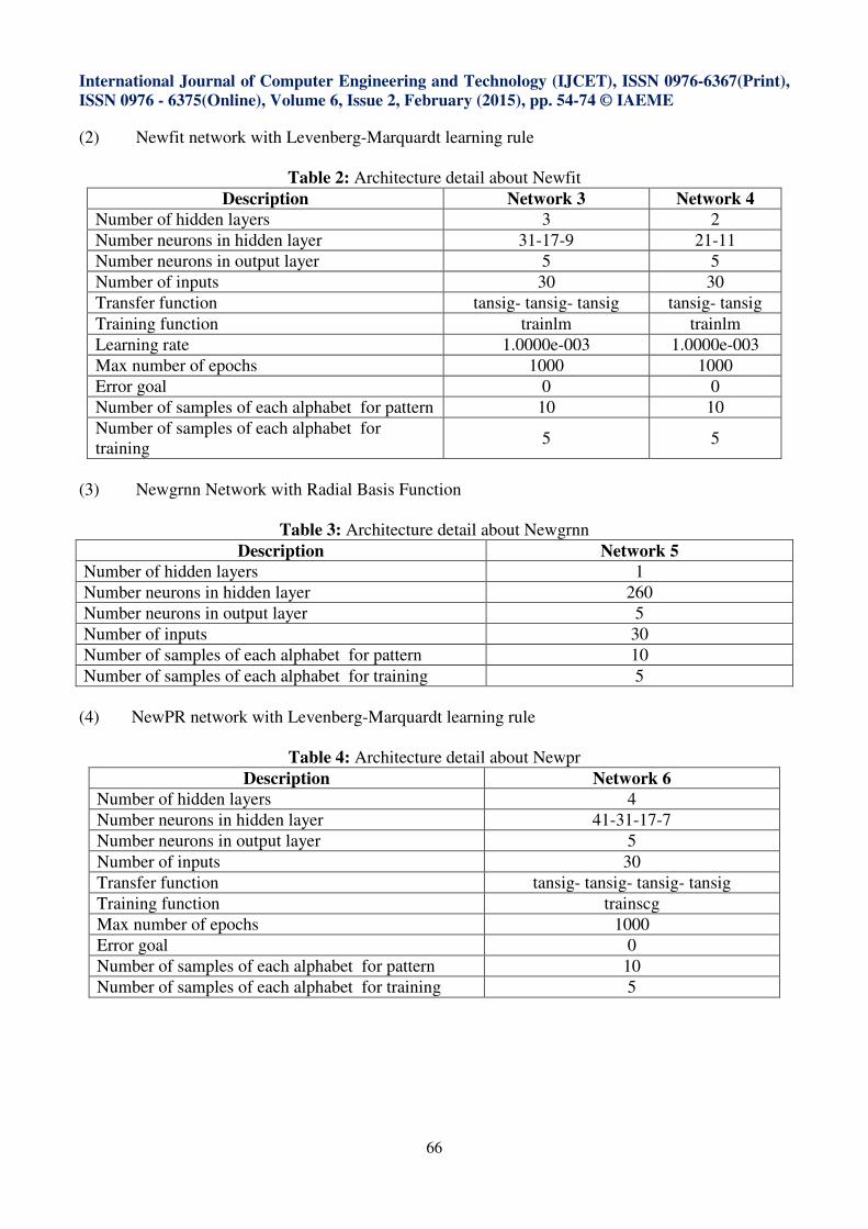
(1) Newff network with Levenberg-Marquardt learning rule
Table 1: Architecture detail about Newff
Description Network 1 Network 2
Number of hidden layers 3 2
Number neurons in hidden layer 37-23-7 21-11
Number neurons in output layer 5 5
Number of inputs 30 30
Transfer function tansig- tansig- tansig tansig- tansig
Training function trainlm trainlm
Learning rate 1.0000e-003 1.0000e-003
Max number of epochs 1000 1000
Error goal 0 0
Number of samples of each alphabet for pattern 10 10
Number of samples of each alphabet for training 5 5
International Journal of Computer Engineering and Technology (IJCET), ISSN 0976-6367(Print),
ISSN 0976 - 6375(Online), Volume 6, Issue 2, February (2015), pp. 54-74 © IAEME
66
(2) Newfit network with Levenberg-Marquardt learning rule
Table 2: Architecture detail about Newfit
Description Network 3 Network 4
Number of hidden layers 3 2
Number neurons in hidden layer 31-17-9 21-11
Number neurons in output layer 5 5
Number of inputs 30 30
Transfer function tansig- tansig- tansig tansig- tansig
Training function trainlm trainlm
Learning rate 1.0000e-003 1.0000e-003
Max number of epochs 1000 1000
Error goal 0 0
Number of samples of each alphabet for pattern 10 10
Number of samples of each alphabet for
training 5 5
(3) Newgrnn Network with Radial Basis Function
Table 3: Architecture detail about Newgrnn
Description Network 5
Number of hidden layers 1
Number neurons in hidden layer 260
Number neurons in output layer 5
Number of inputs 30
Number of samples of each alphabet for pattern 10
Number of samples of each alphabet for training 5
(4) NewPR network with Levenberg-Marquardt learning rule
Table 4: Architecture detail about Newpr
Description Network 6
Number of hidden layers 4
Number neurons in hidden layer 41-31-17-7
Number neurons in output layer 5
Number of inputs 30
Transfer function tansig- tansig- tansig- tansig
Training function trainscg
Max number of epochs 1000
Error goal 0
Number of samples of each alphabet for pattern 10
Number of samples of each alphabet for training 5
International Journal of Computer Engineering and Technology (IJCET), ISSN 0976-6367(Print),
ISSN 0976 - 6375(Online), Volume 6, Issue 2, February (2015), pp. 54-74 © IAEME
67
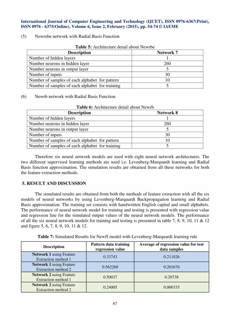
(5) Newrebe network with Radial Basis Function
Table 5: Architecture detail about Newrbe
Description Network 7
Number of hidden layers 1
Number neurons in hidden layer 260
Number neurons in output layer 5
Number of inputs 30
Number of samples of each alphabet for pattern 10
Number of samples of each alphabet for training 5
(6) Newrb network with Radial Basis Function
Table 6: Architecture detail about Newrb
Description Network 8
Number of hidden layers 1
Number neurons in hidden layer 260
Number neurons in output layer 5
Number of inputs 30
Number of samples of each alphabet for pattern 10
Number of samples of each alphabet for training 5
Therefore six neural network models are used with eight neural network architectures. The
two different supervised learning methods are used i.e. Levenberg-Marquardt learning and Radial
Basis function approximation. The simulation results are obtained from all these networks for both
the feature extraction methods.
5. RESULT AND DISCUSSION
The simulated results are obtained from both the methods of feature extraction with all the six
models of neural networks by using Levenberg-Marquardt Backpropagation learning and Radial
Basis approximation. The training set consists with handwritten English capital and small alphabets.
The performance of neural network model for training and testing is presented with regression value
and regression line for the simulated output values of the neural network models. The performance
of all the six neural network models for training and testing is presented in table 7, 8, 9, 10, 11 & 12
and figure 5, 6, 7, 8, 9, 10, 11 & 12.
Table 7: Simulated Results for Newff model with Levenberg-Marquardt learning rule
Description Pattern data training
regression value
Average of regression value for test
data samples
Network 1 using Feature
Extraction method 1 0.33743 0.211826
Network 1 using Feature
Extraction method 2 0.562268 0.201676
Network 2 using Feature
Extraction method 1 0.50037 0.20738
Network 2 using Feature
Extraction method 2 0.24005 0.000335
International Journal of Computer Engineering and Technology (IJCET), ISSN 0976-6367(Print),
ISSN 0976 - 6375(Online), Volume 6, Issue 2, February (2015), pp. 54-74 © IAEME
68
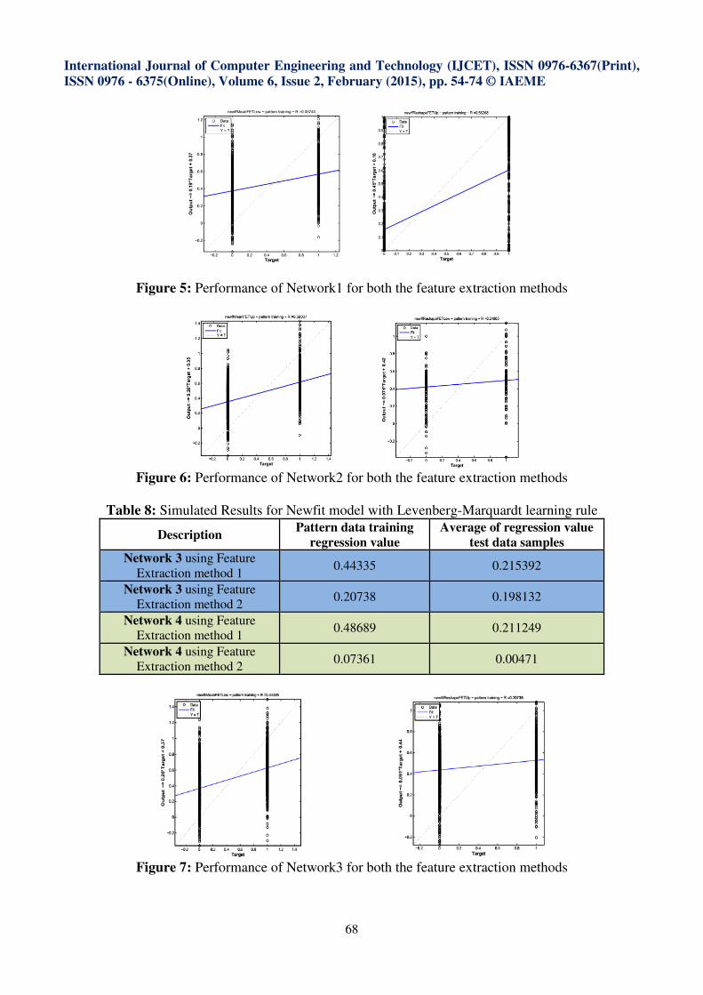
Figure 5: Performance of Network1 for both the feature extraction methods
Figure 6: Performance of Network2 for both the feature extraction methods
Table 8: Simulated Results for Newfit model with Levenberg-Marquardt learning rule
Description Pattern data training
regression value
Average of regression value
test data samples
Network 3 using Feature
Extraction method 1 0.44335 0.215392
Network 3 using Feature
Extraction method 2 0.20738 0.198132
Network 4 using Feature
Extraction method 1 0.48689 0.211249
Network 4 using Feature
Extraction method 2 0.07361 0.00471
Figure 7: Performance of Network3 for both the feature extraction methods
International Journal of Computer Engineering and Technology (IJCET), ISSN 0976-6367(Print),
ISSN 0976 - 6375(Online), Volume 6, Issue 2, February (2015), pp. 54-74 © IAEME
69
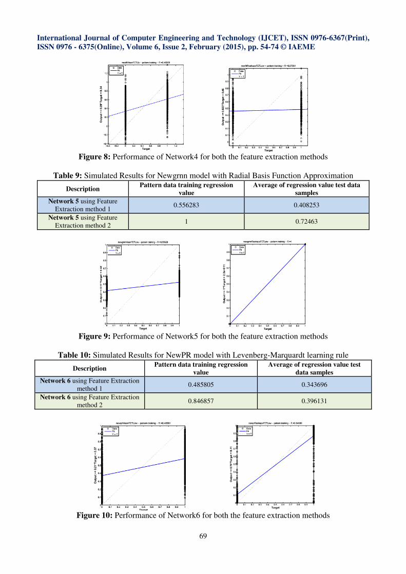
Figure 8: Performance of Network4 for both the feature extraction methods
Table 9: Simulated Results for Newgrnn model with Radial Basis Function Approximation
Description Pattern data training regression
value
Average of regression value test data
samples
Network 5 using Feature
Extraction method 1 0.556283 0.408253
Network 5 using Feature
Extraction method 2 1 0.72463
Figure 9: Performance of Network5 for both the feature extraction methods
Table 10: Simulated Results for NewPR model with Levenberg-Marquardt learning rule
Description Pattern data training regression
value
Average of regression value test
data samples
Network 6 using Feature Extraction
method 1 0.485805 0.343696
Network 6 using Feature Extraction
method 2 0.846857 0.396131
Figure 10: Performance of Network6 for both the feature extraction methods

International Journal of Computer Engineering and Technology (IJCET), ISSN 0976-6367(Print),
ISSN 0976 - 6375(Online), Volume 6, Issue 2, February (2015), pp. 54-74 © IAEME
70
Table 11: Simulated Results for Newrbe model with Radial Basis Function Approximation
Description Pattern data training
regression value
Average of regression value test
data samples
Network 7 using Feature Extraction
method 1 1 0.403733
Network 7 using Feature Extraction
method 2 1 0.112004
Figure 11: Performance of Network7 for both the feature extraction methods
Table 12: Simulated Results for Newrb model with Radial Basis Function Approximation
Description Pattern data training
regression value
Average of regression
value test data samples
Network 8 using Feature Extraction
method 1 1 0.303037
Network 8 using Feature Extraction
method 2 1 0.112487
Figure 12: Performance of Network 8 for both the feature extraction methods
The simulation results of training are indicating that the performance of network models with
Radial Basis function approximation is better than network models with Levenberg-Marquardt
International Journal of Computer Engineering and Technology (IJCET), ISSN 0976-6367(Print),
ISSN 0976 - 6375(Online), Volume 6, Issue 2, February (2015), pp. 54-74 © IAEME
71
Backpropagation learning technique for the second feature extraction method i.e. each pixel value of
the resize and processed image. Now we evaluate the performance of these trained neural network
models for reorganization of handwritten English capital and small alphabets, those did not present
during the training. The performances of these networks are presented in table 13 and table 14. The
table 13 is presenting the performance of all the six neural network models for the prototype input
patterns processed with first method of feature extraction whereas the table 14 is presenting the
performance of all he six neural network models for the same input patterns processed with second
method of feature extraction. The first row of both the tables is representing the rate of correct
recognition for the presented input patterns. The second row of both the tables is presenting the
correct number of recognized pattern among the presented arbitrary patterns.
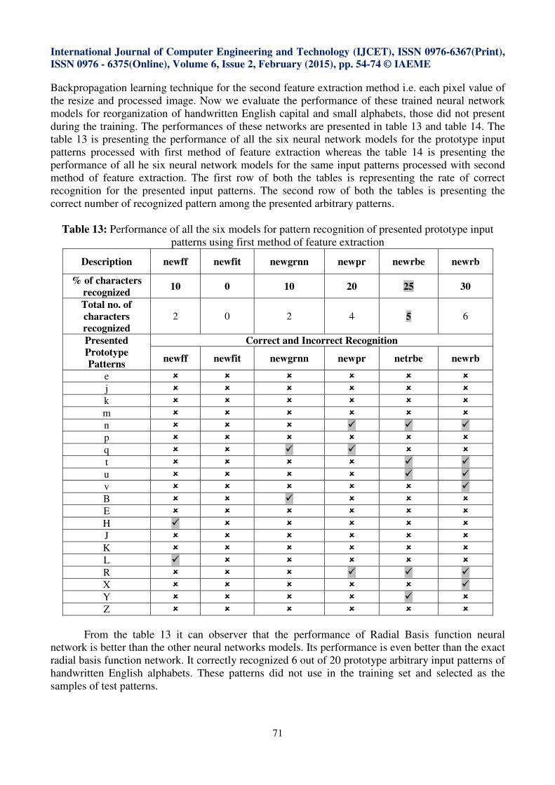
Table 13: Performance of all the six models for pattern recognition of presented prototype input
patterns using first method of feature extraction
Description newff newfit newgrnn newpr newrbe newrb
% of characters
recognized 10 0 10 20 25 30
Total no. of
characters
recognized
2 0 2 4 5 6
Presented
Prototype
Patterns
Correct and Incorrect Recognition
newff newfit newgrnn newpr netrbe newrb
e � � � � � �
j � � � � � �
k � � � � � �
m � � � � � �
n � � � � � �
p � � � � � �
q � � � � � �
t � � � � � �
u � � � � � �
v � � � � � �
B � � � � � �
E � � � � � �
H � � � � � �
J � � � � � �
K � � � � � �
L � � � � � �
R � � � � � �
X � � � � � �
Y � � � � � �
Z � � � � � �
From the table 13 it can observer that the performance of Radial Basis function neural
network is better than the other neural networks models. Its performance is even better than the exact
radial basis function network. It correctly recognized 6 out of 20 prototype arbitrary input patterns of
handwritten English alphabets. These patterns did not use in the training set and selected as the
samples of test patterns.
International Journal of Computer Engineering and Technology (IJCET), ISSN 0976-6367(Print),
ISSN 0976 - 6375(Online), Volume 6, Issue 2, February (2015), pp. 54-74 © IAEME
72
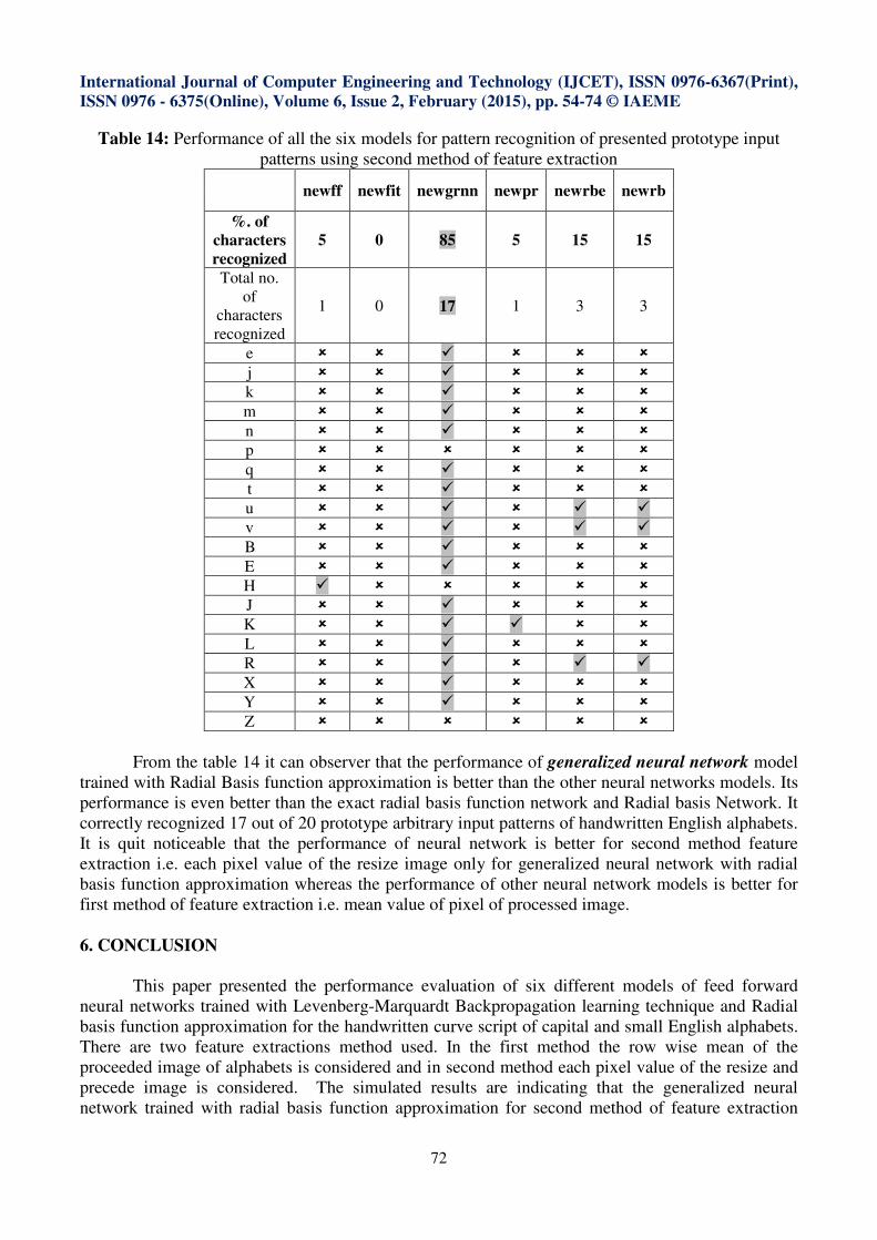
Table 14: Performance of all the six models for pattern recognition of presented prototype input
patterns using second method of feature extraction
newff newfit newgrnn newpr newrbe newrb
%. of
characters
recognized
5 0 85 5 15 15
Total no.
of
characters
recognized
1 0 17 1 3 3
e � � � � � �
j � � � � � �
k � � � � � �
m � � � � � �
n � � � � � �
p � � � � � �
q � � � � � �
t � � � � � �
u � � � � � �
v � � � � � �
B � � � � � �
E � � � � � �
H � � � � � �
J � � � � � �
K � � � � � �
L � � � � � �
R � � � � � �
X � � � � � �
Y � � � � � �
Z � � � � � �
From the table 14 it can observer that the performance of generalized neural network model
trained with Radial Basis function approximation is better than the other neural networks models. Its
performance is even better than the exact radial basis function network and Radial basis Network. It
correctly recognized 17 out of 20 prototype arbitrary input patterns of handwritten English alphabets.
It is quit noticeable that the performance of neural network is better for second method feature
extraction i.e. each pixel value of the resize image only for generalized neural network with radial
basis function approximation whereas the performance of other neural network models is better for
first method of feature extraction i.e. mean value of pixel of processed image.
6. CONCLUSION
This paper presented the performance evaluation of six different models of feed forward
neural networks trained with Levenberg-Marquardt Backpropagation learning technique and Radial
basis function approximation for the handwritten curve script of capital and small English alphabets.
There are two feature extractions method used. In the first method the row wise mean of the
proceeded image of alphabets is considered and in second method each pixel value of the resize and
precede image is considered. The simulated results are indicating that the generalized neural
network trained with radial basis function approximation for second method of feature extraction
International Journal of Computer Engineering and Technology (IJCET), ISSN 0976-6367(Print),
ISSN 0976 - 6375(Online), Volume 6, Issue 2, February (2015), pp. 54-74 © IAEME
73
yields the highest rate of recognition i.e. 85% for randomly chosen 10 lower case and 10 uppercase
characters. The remaining models of neural networks are showing poor performance irrespective of
the feature extraction method. The following observations are considered from the simulation of
performance evaluation:
1. First method of feature extraction uses 30 features for each character whereas second method
of feature extraction uses 100 features for the each character. Thus, it seems that more the
number of features more is the accuracy level as far as generalized neural network model is
concern.
2. In the training process the regression value for Radial basis network is found perfect but during
the validation for the test pattern the performance degrades rapidly. Thus the network is well
tuned for the training set but not able to generalize the behavior. It is working as good
approximation and bad generalization.
3. The second method of feature extraction is providing more feature values in the pattern
information with respect to the first method of feature extraction. Therefore, the performance
of each neural network model is found better for the second feature extraction method.
7. REFERENCES
1. J. Pradeep, E. Srinivasan and S. Himavathi, “Diagonal based feature extraction for
handwritten alphabets recognition system using neural network”, International Journal of
Computer Science & Information Technology (IJCSIT), 3 (1) 27-38 (2011)
2. R. Plamondon and S. N. Srihari, “On-Line and Off-Line handwriting recognition recognition
– A complete survey”, IEEE Transaction on pattern Recognition and Machine Intelligence,
22 (1) 63-84 (2000)
3. Kauleshwar Prasad, D. C. Nigam, Ashmika Lakhotiya and Dheeren Umre, “Character
Recognition Using Matlab’s Neural Network Toolbox”, International Journal of u- and e-
Service, Science and Technology, 6 (1) 13-20 (2013)
4. Ankit Sharma and Dipti R Chaudhary, “Character Recognition Using Neural Network”,
International Journal of Engineering Trends and Technology (IJETT), 4 (4) 662-667 (2013)
5. Chirag I. Patel, Ripal Patel and Palak Patel, “Handwritten Character Recognition using
Neural Network”, International Journal of Scientific & Engineering Research, 2 (5) 1-6
(2011)
6. Manish Mangal and Manu Pratap Singh, “Handwritten English vowels recognition using
hybrid evolutionary Feed-forward neural network”, Malaysian Journal of Computer Science,
19 (2) 169-187 (2006).
7. Anita pal and Dayashankar Singh, “Handwritten english character recognition using neural
network”, International Journal of Computer Science & Communication, 1 (2) 141-144
(2010).
8. K. Y. Rajput and Sangeeta Mishra, “Recognition and editing of Devnagri handwriting using
neural network”, Proc33dings of SPIT-IEEE Colloquium and International Conference,
Mumbai, India, 1 66-70 (2008)
9. Meenakshi Sharma and Kavita Khanna, “Offline signature verification using supervised and
unsupervised neural networks”, International Journal of Computer Science and Mobile
Computing, 3 (7) 425-436 (2014).
10. Priyanka Sharma and Manavjeet Kaur, “Classification in Pattern Recognition: A Review“,
International Journal of Advanced Research in Computer Science and Software Engineering,
3 (4) 298-306 (2013)
11. K. Fukushima and N. Wake, "Handwritten alphanumeric character recognition by the
neocognitron.", IEEE Trans. on Neural Networks, 2 (3) 355-365 (1991).
International Journal of Computer Engineering and Technology (IJCET), ISSN 0976-6367(Print),
ISSN 0976 - 6375(Online), Volume 6, Issue 2, February (2015), pp. 54-74 © IAEME
74
12. Y. L. Cun, B. Boser, J. S. Denker, D. Henderson, R. E. Howard, W. Hubbad and L. D. Jackel,
"Handwritten digit recognition with a Backpropagation network", Neural Information
Processing Systems, Touretzky editor, Morgan Kaufmann Publishers, (2) 396-404 (1990).
13. A. K. Jain, J. Mao and K. M. Mohiuddin, “Artificial Neural Networks: A Tutorial.”,
Computer, 31-44, (1996).
14. B. Ripley, “Statistical Aspects of Neural Networks.”, Networks on Chaos: Statistical and
Probabilistic Aspects. U. Bornndorff-Nielsen, J. Jensen, and W. Kendal, eds., Chapman and
Hall, (1993).
15. J. Anderson, A. Pellionisz and E. Rosenfeld, “Neuro-computing 2: Directions for Research”,
Cambridge Mass.: MIT Press, (1990).
16. F. Rosenblatt, “Principles of Neurodynamics: Perceptron and the Theory of Brain
Mechanisms”, Spartan Books, Washington, D.C., (1962).
17. B. Widrow and M. A. Lehr, “30 years of adaptive neural networks: perceptron, Madeline, and
Backpropagation.”, Proceedings of the IEEE 78 (9) 1415-1442 (1990).
18. M. L. Minsky and S. A. Papert, “Perceptron.”, Cambridge, MA: MIT Press. Expanded
Edition, (1990).
19. S. B. Cho, “Fusion of neural networks with fuzzy logic and genetic algorithm”, IOS Press,
363–372 (2002).
20. B. Widrow and M. E. Hoff, ”Adaptive switching circuits” IRE Eastern Electronic Show &
Convention (WESCON1960), Convention Record, (4) 96–104 (1960).
21. P. J. Werbos, “Beyond regressions: New tools for prediction and analysis in the behavioral
sciences”, PhD Thesis, Harvard University, Cambridge, MA, (1974).
22. F. J. Pineda, “Generalization of back-propagation to recurrent neural networks”, Physical Rev
Letter, (59) 2229–2232 (1987).
23. R. Battiti, and F. Masulli, “BFGS optimization for faster automated supervised learning”, In:
Proc. Int. Neural Network Conf. France, (2) 757-760 (1990)
24. D. E. Rumelhart, G. E. Hinton and R. J. Williams, “Learning internal representations by error
propagation”, MIT Press, Cambridge, (1) 318–362 (1986).
25. P. Muneesawang and L. Guan, "Image retrieval with embedded sub-class information using
Gaussian mixture models", Proceedings of International Conference on Multimedia and
Expo, (2003).
26. S. Lee. “Off-Line Recognition of Totally Unconstrained Handwritten Numerals Using
Multilayer Cluster Neural Network”, IEEE Trans. Pattern Anal. Mach. Intell. 18 (6) 648-652
(1996).
27. S. Shrivastava, S. and Manu Paratp Singh, “Performance evaluation of feed-forward
neural network with soft computing techniques for hand written English alphabets”,
Journal of Applied Soft Computing, Elsevier, (11) 1156-1182 (2011).
28. V. Subba Ramaiah and R. Rajeswara Rao, “Automatic Text-Independent Speaker Tracking
System Using Feed-Forward Neural Networks (FFNN)” International journal of Computer
Engineering & Technology (IJCET), Volume 5, Issue 1, 2014, pp. 11 - 20, ISSN Print: 0976
– 6367, ISSN Online: 0976 – 6375.
29. M. M. Kodabagi, S. A. Angadi and Chetana. R. Shivanagi, “Character Recognition of
Kannada Text In Scene Images Using Neural Network” International Journal Of Graphics
And Multimedia (IJGM), Volume 4, Issue 1, 2014, pp. 9 - 19, ISSN Print: 0976 – 6448, ISSN
Online: 0976 –6456.
30. Ms. Aruna J. Chamatkar and Dr. P.K. Butey, “Performance Analysis of Data Mining
Algorithms with Neural Network” International journal of Computer Engineering &
Technology (IJCET), Volume 6, Issue 1, 2015, pp. 1 - 11, ISSN Print: 0976 – 6367, ISSN
Online: 0976 – 6375.