5.2 Variable-Amplitude Loading Baseline fatigue data are derived under constant-amplitude loading conditions, but aircraft components are subjected to variable amplitude loading. If there were not interaction effects of high and low loads in the sequence, it would be relatively easy to establish a crack-growth curve by means of a cycle-by-cycle integration. However, interaction effects of high and low loads largely complicate crack-growth under variable-amplitude cycling.

In the following sections these interaction effects will be briefly discussed. Crack growth-prediction procedures that take interaction effects into account will be presented in Section 5.2.3.

5.2.1 Retardation A high load occurring in a sequence of low-amplitude cycles significantly reduces the rate of crack-growth during the cycles applied subsequent to the overload. This phenomenon is called retardation. Figure 5.2.1 shows a baseline crack-growth curve obtained in a constant-amplitude test [Schijve & Broek, 1962]. In other experiments, the same constant-amplitude loading was interspersed with overload cycles. After each application of the overload, the crack virtually stopped growing during many cycles, after which the original crack-growth behavior was gradually restored.

Figure 5.2.1. Retardation Due to Positive Overloads, and Due to Positive-Negative Overload

Cycles [Schijve & Broek, 1962]

5.2.1

Retardation results from the plastic deformations that occur as the crack propagates. During loading, the material at the crack tip is plastically deformed and a tensile plastic zone is formed. Upon load release, the surrounding material is elastically unloaded and a part of the plastic zone experiences compressive stresses. The larger the load, the larger the zone of compressive stresses. If the load is repeated in a constant amplitude sense, there is no observable direct effect of the residual stresses on the crack-growth behavior; in essence, the process of growth is steady state. Measurements have indicated, however, that the plastic deformations occurring at the crack tip remain as the crack propagates so that the crack surfaces open and close at non zero (positive) load levels. These observations have given rise to constant amplitude crack-growth models referred to as closure models [Elber, 1971] after the concept that the crack may be closed during part of the load cycle.

When the load history contains a mix of constant amplitude loads and discretely applied higher level loads, the patterns of residual stress and plastic deformation are perturbed. As the crack propagates through this perturbed zone under the constant amplitude loading cycles, it grows slower (the crack is retarded) than it would have if the perturbation had not occurred. After the crack has propagated through the perturbed zone, the crack growth rate returns to its typical steady state level.

Two basic models have been proposed to describe the phenomenon of crack retardation. The first model is based on the concept of the compressive residual stress perturbation and the second on the concept of plastic deformation with enhanced crack wedging and more closure.

If the tensile overload is followed by a compressive overload, the material at the crack tip may undergo reverse plastic deformation and this reduces the residual stresses. Thus, a negative overload in whole or in part annihilates the beneficial effect of tensile overloads, as is also shown by curve C in Figure 5.2.1.

Retardation depends upon the ratio between the magnitude of the overload and subsequent cycles. This is illustrated in Figure 5.2.2. Sufficiently large overloads may cause total crack arrest. Hold periods at zero stress can partly alleviate residual stresses and thus reduce the retardation effect [Shih & Wei, 1974; Wei & Shih, 1974], while hold periods at load increase retardation. Multiple overloads significantly enhance the retardation. This is shown in Figure 5.2.3.

5.2.2

Figure 5.2.2. Effect of Magnitude of Overload on Retardation [Shih & Wei, 1974]

Figure 5.2.3. Retardation in Ti-6V-4Al; Effect of Hold Periods and Multiple Overloads [Wei &

Shih, 1974]

5.2.3

5.2.1.1 Retardation Under Spectrum Loading

An actual service load history contains high- and low- stress amplitudes and positive and negative “overloads” in random order. Retardation and annihilation of retardation becomes complex, but qualitatively the loading produces behavior that is similar to a constant-amplitude history with incidental overloads. The higher the maximum stresses in the service load history, the larger the retardation effect during the low-amplitude cycles. Negative stress excursions reduce the retardation effect and tend to enhance crack-growth. These effects have been documented in various sources [Schijve, 1972; Schijve, 1970; Wood et al., 1971; Porter, 1972; Potter, et al., 1974; Gallagher et al., 1974; Wood, et al., 1971]; a few examples are now presented.

When the magnitude of the higher loads are reduced (or clipped) without eliminating the cycle, i.e., higher loads are reset to a defined lower level, the cracking rates are observed to speed up as shown in Figure 5.2.4 [Schijve, 1972; Schijve, 1970]. Figure 5.2.4 describes the crack growth life results for a study in which a (random) flight-by-flight stress history was systematically modified by “clipping” the highest load excursions to the three levels shown.

Figure 5.2.4. Effect of Clipping of Higher Loads in Random Flight-by-Flight Loading on Crack

Propagation In 2024-T3 Al Alloy [Schijve, 1972; Schijve, 1970]

In Schijve [1970; 1972], it was also observed that negative stress excursions reduce the retardation effect and omission of the ground-air-ground (G-A-G) cycles (negative loads) in the tests with the highest clipping level resulted in a longer crack growth life for the same amount of crack growth.

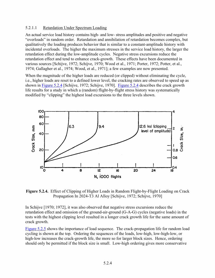
Figure 5.2.5 shows the importance of load sequence. The crack-propagation life for random load cycling is shown at the top. Ordering the sequences of the loads, low-high, low-high-low, or high-low increases the crack-growth life, the more so for larger block sizes. Hence, ordering should only be permitted if the block size is small. Low-high ordering gives more conservative

5.2.4

results than high-low ordering. In the latter case, the retardation effect caused by the highest load is effective during all subsequent cycles.

Figure 5.2.5. Effect of Block Programming and Block Size On Crack Growth Life All Histories

Have Same Cycle Content; Alloy: 2024-T3 Aluminum [Shih & Wei, 1974]

5.2.1.2 Retardation Models

Some mathematical models have been developed to account for retardation in crack-growth-integration procedures. All models are based on simple assumptions, but within certain limitations and when used with experience, each model will produce results that can be used with reasonable confidence. The two yield zone models by Wheeler [1972] and by Willenborg, et al., [1971], and a crack-closure model by Bell & Creager [1975] will be briefly discussed. Detailed information and applications of closure models can be found in Bell & Creager [1975], Rice & Paris [1976], Chang & Hudson [1981], and Wei & Stephens [1976].

Wheeler Model Wheeler defines a crack-growth reduction factor, Cp:

)K(fCdNda

pr

∆=

(5.2.1)

5.2.5

where f(∆K) is the usual crack-growth function, and (da/dN) is the retarded crack-growth rate. The retardation factor, Cp is given as

m

ipoLoL

pip ara

rC

−+= (5.2.2)

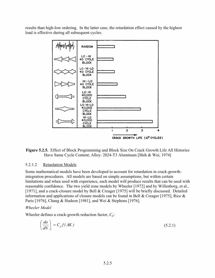
where (see Figure 5.2.6):

aOL

ai Rpi

rpOL

Overload

Plastic Zone

Current

Plastic Zone

Current Crack Position

Crack Position when Overload Applied

rpi – current plastic zone size in the ith cycle under consideration ai – current crack size rpoL – plastic size generated by a previous higher load excursion aoL – crack size at which the higher load excursion occurred m – empirical constant

Figure 5.2.6. Yield Zone Due to Overload (rpoL), Current Crack Size (ai), and Current Yield

Zone (rpi)

There is retardation as long as the current plastic zone (rpi) is contained within a previously generated plastic zone (rpoL) ; this is the fundamental assumption of yield zone models.

Some examples of crack-growth predictions made by means of the Wheeler model are shown in Figure 5.2.7. Selection of the proper value for the exponent m will yield adequate crack-growth predictions. In fact, one of the earlier advantages of the Wheeler model was that exponent m could be tailored to allow for reasonably accurate life predictions of spectrum test results. Through the course of time, it has become recognized, however, that the exponent m was dependent on material, crack size, and stress-intensity factor level as well as spectrum. The reader is cautioned against using the Wheeler model for service life predictions based on limited amounts of supporting test data and more specifically against estimating the service life of structures with spectra radically different from those for which the exponent m was derived. Estimates made without the supporting data required to tailor the exponent m can lead to inaccurate and unconservative results.

5.2.6

Figure 5.2.7. Crack Growth Predictions by Wheeler Model Using Different Retardation

Exponents [Wood, et al. 1971]

Willenborg Model The Willenborg model also relates the magnitude and extent of the retardation factor to the overload plastic zone. The extent of the retardation is handled exactly the same as that of the Wheeler model. The magnitude of the retardation factor is established through the use of an effective stress-intensity factor that senses the differences in compressive residual stress state caused by differences in load levels. The effective stress-intensity factor (Keff

i) is equal to the typical remote stress-intensity factor (Ki) for the ith cycle minus the residual stress-intensity factor (KR):

Rieff

i KKK −= (5.2.3)

where in the original formulation [Willenborg, et al., 1971; Gallagher, 1974; Gallagher & Hughes, 1974; Wood, 1974]

imax,poL

oLioLmax

WRR K

raaKKK −

−−== 1 (5.2.4)

in which (see Figure 5.2.6):

ai – current crack size

aoL –- crack size at the occurrence of the overload

rpoL – yield zone produced by the overload

KoLmax – maximum stress intensity of the overload

Kmax,i – maximum stress intensity for the current cycle.

5.2.7

The equations show that retardation will occur until the crack has generated a plastic zone size that reaches the boundary of the overload yield zone. At that time, ai-aoL= rpoL and the reduction becomes zero.

Equation 5.2.3 indicates that the complete stress-intensity factor cycle, and therefore, its maximum and minimum levels (Kmax, i and Kmin, i), are reduced by the same amount (KR). Thus, the retardation effect is sensed by the change in the effective stress ratio calculated by

Rimax,

Rimin,eff

imax,

effimin,

eff KKKK

KK

R−−

== (5.2.5)

since the range in stress-intensity factor is unchanged by the uniform reduction. Thus, for the ith load cycle, the crack growth increment (∆ai) is:

( )effi RKfdNdaa ,∆==∆ (5.2.6)

For many of the early calculations with the Willenborg model, it was assumed that Reff was never less than zero and that when Reff

iKK max,=∆ eff was calculated to be less than zero. Recent evidence, however, supports the calculations of Reff as given by Equation 5.2.5 and the use of a negative stress ratio cut-off in the crack growth rate calculation (Equation 5.2.6) for more accurate modeling of crack growth behavior.

Another problem that was identified with the original Willenborg model was that it was always assigned the same level of residual stress effect independent of the type of loading. In particular, it can be noted (through the use of Equation 5.2.3 and 5.2.4) that the model predicts that

, and therefore crack arrest, immediately after overload if . That is, if the overload is twice as large as (or larger than) the following loads, the crack arrests. To account for the observations of continuing crack propagation after overloads larger than a factor of two or more, Gallagher & Hughes [1974] introduced an empirical (spectra/material) constant into the calculations. Specifically, they suggested that

0max, =effiK imax,

oLmax K K 2=

WRR KK φ= (5.2.7)

where φ is given by

1

1max,

max,

−

−= oL

i

th

SKK

φ (5.2.7a)

There are two empirical constants in Equation 5.2.7a: Kmax, th is the threshold stress-intensity factor level associated with zero fatigue crack growth rates (see Section 5.1.2), and S

oL is the overload (shut-off) ratio required to cause crack arrest for the given material. The type of underload/overload cycle, as well as the frequency of overload cycle occurrence, affects this ratio. Results of some life predictions made using what has become to be called the “Generalized” Willenborg model are presented in Figure 5.2.8 [Engle & Rudd, 1974]. Compressive stress levels were ignored in this analysis.

5.2.8

Figure 5.2.8. Predictions of Crack Growth Lives with the Generalized Willenborg Model

Compared to Test Data [Engle & Rudd, 1974]

Closure Models One of the earliest crack-closure models developed for aircraft structural applications is attributed to Bell & Creager [1975]. The closure model makes use of a crack-growth-rate equation based on an effective stress-intensity range ∆Keff. The effective stress intensity is the difference between the applied stress intensity and the stress intensity for crack closure. Some examples of predictions made with the model are presented in Figure 5.2.9. The final equations contain many experimental constants, which reduces the versatility of the model and make it difficult to apply. Recent work by Dill & Saff [1977] shows that the closure model can be simplified to the point of practicality while retaining a high level of accuracy in life prediction.

5.2.9

Figure 5.2.9. Predictions by Crack Growth Closure Model as Compared with Data Resulting

From Constant-Amplitude Tests with Overload Cycles [Bell & Creager, 1975]

Crack-growth calculations are the most useful for comparative studies, where variations of only a few parameters are considered (i.e., trade-off studies to determine design details, design stress levels, material selection, etc.). The predictions must be verified by experiments. (See Analysis Substantiation Tests in Section 7.3). Example calculations of crack-growth curves will be given in Section 5.5.

Other factors contributing to uncertainties in crack-growth predictions are:

• Scatter in baseline da/dN data,

• Unknowns in the effects of service environment,

• Necessary assumptions on flaw shape development,

• Deficiencies in K calculation,

• Assumptions on interaction of cracks,

• Assumptions on service stress history.

In view of these additional shortcomings of crack-growth predictions, the shortcomings of a retardation model become less pronounced; therefore, no particular retardation model has preference over the others. From a practical point of view, the Generalized Willenborg model is easier to use since it contains a minimum number of empirical constants.

5.2.10

5.2.2 Integration Routines The determination of a crack growth increment due to any particular stress history depends upon an integration of the growth rate relation such as given by equations 5.1.2 - 5.1.4. Four general methods are available for this purpose.

The first approach is based on extensive spectrum crack growth data. Tests that incorporate the important stress levels, part geometry, crack shape details and loading sequences are run to determine the effect of the particular variables of interest on the component life.

A second approach, and one used extensively, is the cycle-by-cycle crack growth analysis where crack rates are integrated over the crack length of interest as a function of stress and crack length [Gallagher, 1976; Brussat, 1971].

A third approach is based on the statistical stress-parameter-characterization. The actual service stress histories are replaced with equivalent constant amplitude stress histories for the analytical prediction of component life [Smith, et al., 1968].

A fourth approach, recently developed, utilizes a crack-incrementation scheme to analytically generate “mini-block” crack growth rate behavior prior to predicting life. It combines some features of the first three methods [Gallagher, 1976; Brussat, 1971; Gallagher & Stalwaker, 1975].

The application of the second through fourth approaches requires methods for integrating the crack growth rate relations requires the knowledge of the following items:

• An initial flaw distribution

• The aircraft loading spectrum

• Constant amplitude crack growth rate material properties

• Crack tip stress-intensity factor analysis

• A damage integrator model relating crack growth to applied stress and which accounts for load-history interactions

• The criteria which establishes the life-limiting end point of the calculation

These items are described in detail in Section 1.5 of this handbook. The basic damage integrating equation is also presented as equation 1.5.1 but is repeated here:

j

t

ljocr aaa

f

∆∑=

+= (1.5.1R)

where ∆aj is the growth increment associated with the jth time increment, ao is the initial crack length, acr is the critical crack length and tf is the life of the structure. The determination of tf is the objective of this equation.

Of the integration methods described above, the second and third are most frequently used. The generation of the data required for the first method is very expensive and is only recommended for extremely critical parts.

5.2.11

Cycle-by-cycle method The second method, the cycle-by-cycle integration method, uses a type of integrating relation whereby the effect of each cycle is considered separately. This is generally the least efficient method, but if the spectrum under consideration cannot be considered as statistically repetitive, it may be the most accurate of the analytical methods. This method is covered in detail in subsection 5.2.3.

Statistical Stress-Parameter Characterization The third method, using a statistical characterization of a crack growth parameter is based on the similarity of certain variable amplitude crack growth behavior to the constant amplitude function relationship:

( )pKC

dFda

= (5.2.8)

where (da/dF) is the flight-by-flight crack growth behavior and K is a stress-intensity factor parameter that is derived using the product of a statistically characterizing stress parameter σ( ) and the stress-intensity factor coefficient (K/σ), i.e.,

)/( σσ KK ⋅= (5.2.9)

The statistically characterizing parameters that have been employed in the past to some success are derived using a root mean square (RMS) or similar type analysis of the stress range or stress maximum. The crack growth behavior of both fighter and transport aircraft stress histories have been described using various forms of equation 5.2.8.

One might imply from equations 5.2.8 and 5.2.9 that the use of a single stress characterizing parameter for stress histories would allow one to utilize equivalent constant amplitude histories to derive the same crack growth rate behavior. Unfortunately, relating constant amplitude behavior to variable amplitude behavior has not been that successful.

The damage integration Equation (1.5.1R) is now expressed for the flight as

j

N

jok aaa

f

∆+= ∑=1

(5.2.10)

where Nf is the number of flights corresponding to crack length ak, and ∆aj is computed from Equation 5.2.8 evaluated for the given conditions. The parameters C and p of Equation 5.2.8 are determined by a least squares curve fit to previously determined data. The value that comes from employing the third method comes from the fact that a somewhat limited variable amplitude data base might be extended to cover other crack lengths, structural geometry, or stress level differences.

Crack-Incrementation Scheme The fourth approach provides an analytical extension of the cycle-by-cycle analysis to predict flight-by-flight crack growth rates. In essence, this approach combined some of the best features of the other three methods. The basic element in this analysis is what is referred to as a mini-block which is taken to be a flight (includes takeoff, landing and all intermediate stress events) or

5.2.12

a group of flights. The approach hinges on the identification of the statistically repeating stress group that approximates the loading and sequence effects for the complete spectrum.

The basic damage integration equation can be written in the mini-block form to compute the crack increment (∆a) due to application of NG flights:

( )i

N

i

N

jok aaaa

jG

∆=−=∆ ∑∑== 11

(5.2.11)

where there are Nj stress cycles in the jth flight. The most direct method for applying the equation is called the simple crack-incrementation-mini-block approach. Successive crack increments are obtained at successively larger initial-crack-lengths. Figure 5.2.10 illustrates this method. The resulting values of ∆a/∆F and the corresponding Kmax values are fit with a curve of the desired type, usually similar to Equation 5.2.8, which can now be used to compute life.

Figure 5.2.10. Simple Crack-Incrementation Scheme Used to Determine Crack Growth Rate

Behavior [Gallagher, 1976]

An alternate method, called the statistical crack-incrementation-mini-block approach, is illustrated in Figure 5.2.11. This method allows evaluation of the effect of mini-block group-to-group variation in the crack growth rate behavior. A number of different mini-block groups are used at each initial crack length. A curve can be fit through the mean ∆a/∆F vs. maxK values and the variation of ∆a/∆F at each Kmax can be observed. Confidence limits can be determined for each set of data.

5.2.13

Figure 5.2.11. Statistical Crack-Incrementation Scheme Used to Determine Spectrum Induced

Variations in Crack Growth-Rate Behavior [Gallagher, 1976]

The fourth approach provides a more efficient integration scheme than the cycle-by-cycle analysis. However, its use is determined by the type of stress history that has to be integrated.

Summary In summary, there are a number of integration schemes available. These schemes all employ modeling approaches based on either limited or extensive variable amplitude databases so that the analyst might properly account for loading and sequence effects in the most direct and most accurate manner.

5.2.3 Cycle-by-Cycle Analysis Several computer programs are available for general uses that include one or more of the retardation models in a crack-growth-integration scheme. These are discussed in Section 1.7. The user has the option of using any of the retardation models discussed in the previous section. Most airframe companies, however, have their own in-house computer program for performing variable-amplitude fatigue life calculations.

In general, the crack-growth-damage-integration procedure consists of the following steps, schematically outlined in Figure 5.2.12.

5.2.14

Figure 5.2.12. Steps Required for Crack Growth Integration

Step 1. The initial crack size follows from the damage tolerance assumptions as a1. The stress range in the first cycle is ∆σ1. Then determine 111 aK πσ∆β∆ = by using the appropriate β for the given structural geometry and crack geometry. Computer programs generally have a library of stress-intensity factors or schemes for tabular data input for determining the appropriate β.

Step 2. Determine (da/dN)1, at ∆K1 from the da/dN -∆K baseline information, taking into account the appropriate R value. The da/dN - ∆K baseline information may use one of the crack growth equations discussed in Section 5.1.2. The computer program may contain options for any of these equations, or it may use data in tabular form and interpolate between data points. The crack extension ∆a1 in cycle 1 is

⋅×

= 1

dNdaa

11∆

The new crack size will be a2 = a1 + ∆a1

5.2.15

Step 3. The extent of the yield zone in Cycle 1 is determined as

Y pLoL ra +=2

where a = 1aoL

2

1max,

21

=

yspL

Kσπ

r for plane stress

or 2

1max,

241

yspL

Kσπ

=r for plane strain.

Step 4. The crack size is now a2. The stress range in the next cycle is ∆σ2. Calculate ∆K with

222 aK πσ∆β=∆ .

Step 5. Calculate the extent of the yield zone Y22 = a2 + rp2 .

Step 6. If Y22 < Y2:

When using the Wheeler model, calculate Cp according to Equation 5.2.2.

When using the Generalized Willenborg model, calculate or and R effmaxK eff

minK eff according to Equations 5.2.3, and 5.2.5.

Go to Step 9, skipping steps 7 and 8.

Step 7. If Y22 > Y2, determine (da/dN)2 from ∆K2. Determine the new crack size a3

.dNdaaaa 1

22223 ×

+=+= ∆a

Step 8. Replace Y2 by Y22 , which is now called Y2. Replace aoL =a1 with aoL =a2. Go to Step 10, skipping Step 9.

Step 9. When using the Wheeler model, determine the amount of crack growth on the basis of ∆K2 from the da/dN - ∆K data. Find the new crack size from

.dNdaCaa p 1

2223 ×

++= ∆a

When using the Generalized Willenborg model, determine the amount of crack growth using the ∆K and Reff value determine in Step 6 from the da/dN - ∆K data. Determine the new crack size as

12

2223 ×

+=+=

dNdaaaa ∆a

Step 10. Repeat Steps 4 through 9 for every following cycle, while for the ith cycle replacing a2 by ai and a3 by ai+1.

5.2.16

This routine of cycle-by-cycle integration is not always necessary. The integration is faster if the crack size is increased stepwise in the following way.

• At a certain crack size, the available information is ai, aoL, Y2.

• Calculate ∆ai for the ith cycle in the same way as in Steps 4 through 9.

• Calculate ∆aj+1, . . . , ∆aj, . . . , ∆an for the following cycles but let the current crack size remain ai constant. This eliminates recalculation of β every cycle.

• Calculate Y2k for every cycle. If Y2k > Y2, then replace Y2 by Y2k and call it Y2. Then replace aoL by ai and call it aoL.

• Sum the crack-growth increments to give:

⋅∆=∆ ∑=

k

j

ikaa

• Continue increasing j until ∆a exceeds a previously determined size or until j = n and the cycles are exhausted. Then increment the crack size by

a= ai + ∆a,

and repeat the procedure.

A reasonable size for the crack-growth increment is ∆a = 1/20 ai; this choice of increment typically keeps the change in K small. It can also be based on the extent of the yield zone, e.g., ∆a = 1/10 (Y2 - ai). The advantage of the incremental crack-growth procedure is especially obvious if series of constant-amplitude cycles occur. Since the crack size (ai) is fixed, the stress intensity does not change. Hence, each cycle produces the same amount of growth. This means that all n constant-amplitude cycles can be treated as one cycle to give

dNdana =∆

The integration scheme is a matter of individual judgment, but may be dictated by available computer facilities.

5.2.17