5. Statistical Inference: Estimation

Goal: Use sample data to estimate values of population parameters

Point estimate: A single statistic value that is the “best guess” for the parameter value

Interval estimate: An interval of numbers around the point estimate, that has a fixed “confidence level” of containing the parameter value. Called a confidence interval.

Point Estimators – Most common to use sample values

• Sample mean estimates population mean

• Sample std. dev. estimates population std. dev.

• Sample proportion estimates population proportion

Properties of good estimators

• Unbiased: Sampling dist of estimator centers around parameter value

• Efficient: Smallest possible standard error, compared to other estimators

Confidence Intervals

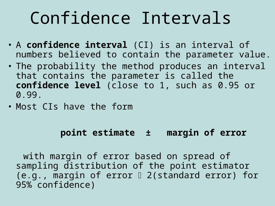
• A confidence interval (CI) is an interval of numbers believed to contain the parameter value.

• The probability the method produces an interval that contains the parameter is called the confidence level (close to 1, such as 0.95 or 0.99.

• Most CIs have the form

point estimate ± margin of error

with margin of error based on spread of sampling distribution of the point estimator (e.g., margin of error 2(standard error) for 95% confidence)

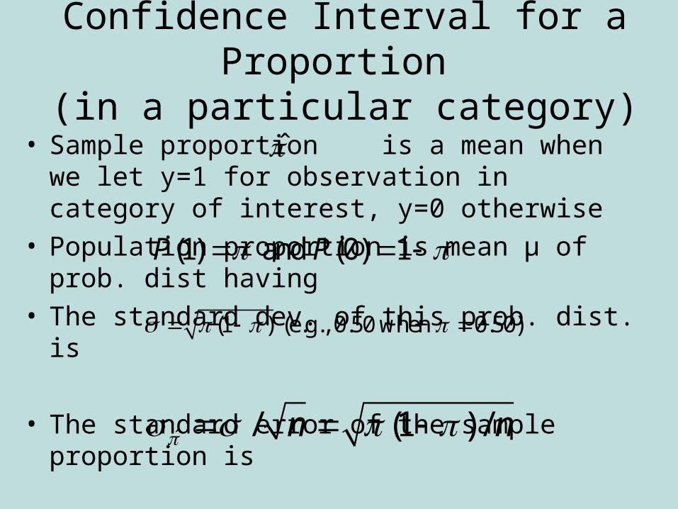
Confidence Interval for a Proportion

(in a particular category)• Sample proportion is a mean when we let y=1 for

observation in category of interest, y=0 otherwise• Population proportion is mean µ of prob. dist

having• The standard dev. of this prob. dist. is

• The standard error of the sample proportion is

(1) and (0) 1P P

(1 ) (e.g., 0.50 when 0.50)

ˆ / (1 ) /n n

• Sampling distribution of sample proportion for large random samples is approximately normal (CLT)

• So, with probability 0.95, sample proportion falls within 1.96 standard errors of population proportion

• 0.95 probability that

• Once sample selected, we’re 95% confident

ˆ ˆˆ falls between 1.96 and 1.96

ˆ ˆˆ ˆ1.96 to 1.96 contains

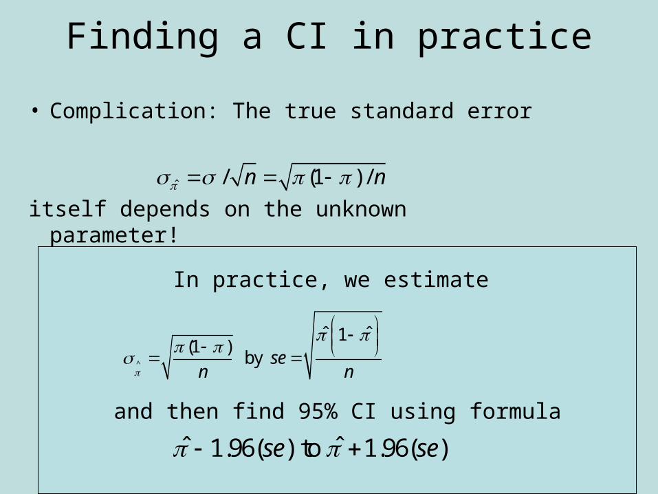
Finding a CI in practice

• Complication: The true standard error

itself depends on the unknown parameter!

ˆ / (1 ) /n n

In practice, we estimate

and then find 95% CI using formula

^

ˆ ˆ1(1 )

by sen n

ˆ ˆ1.96( ) to 1.96( )se se

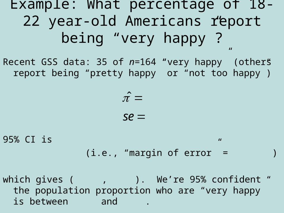
Example: What percentage of 18-22 year-old Americans report being “very happy”?

Recent GSS data: 35 of n=164 “very happy” (others report being “pretty happy” or “not too happy”)

95% CI is

(i.e., “margin of error” = )

which gives ( , ). We’re 95% confident the population proportion who are “very happy” is between and .

ˆ

se

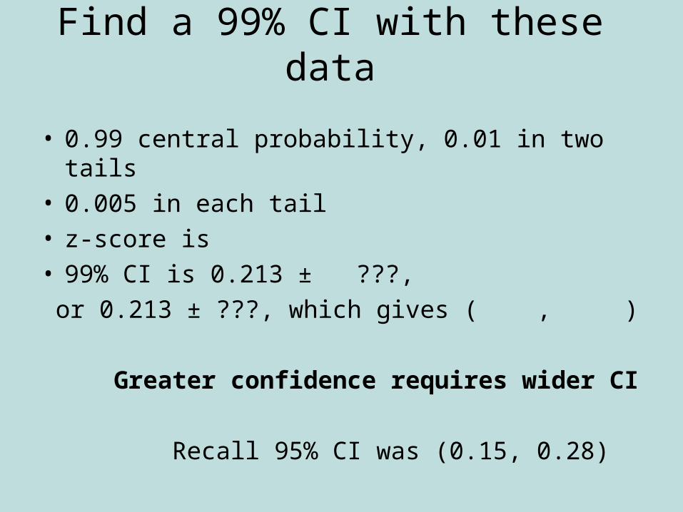
Find a 99% CI with these data

• 0.99 central probability, 0.01 in two tails• 0.005 in each tail• z-score is • 99% CI is 0.213 ± ???,

or 0.213 ± ???, which gives ( , )

Greater confidence requires wider CI

Recall 95% CI was (0.15, 0.28)

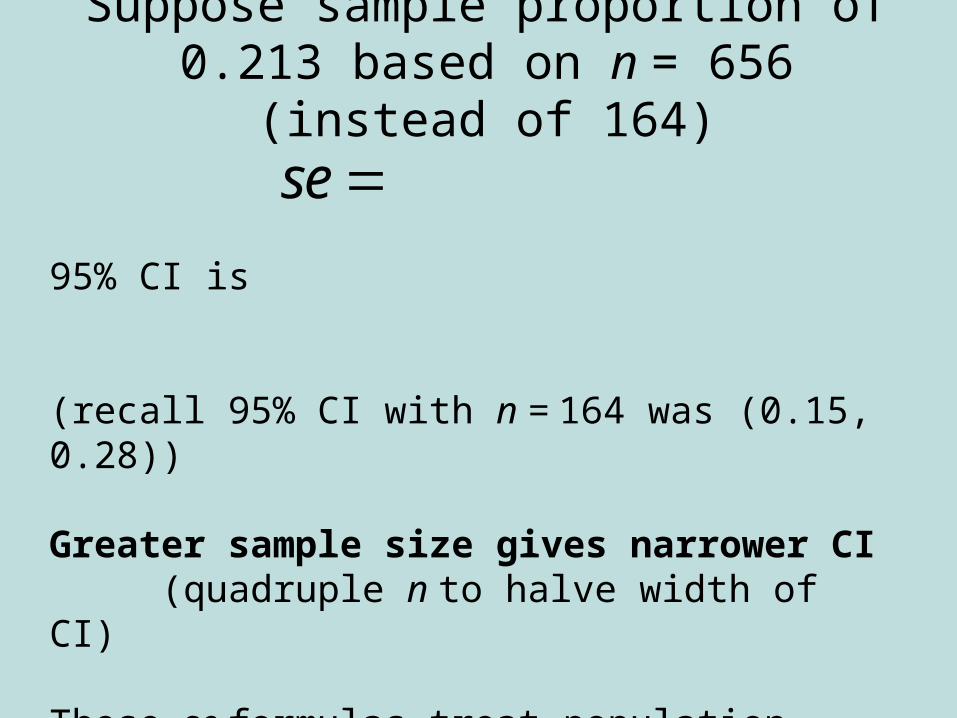
Suppose sample proportion of 0.213 based on n = 656 (instead of 164)

se

95% CI is

(recall 95% CI with n = 164 was (0.15, 0.28))

Greater sample size gives narrower CI (quadruple n to halve width of CI)

These se formulas treat population size as infinite (see Exercise 4.57 for finite population correction)

Some comments about CIs• Effects of n, confidence coefficient true for CIs for

other parameters also• If we repeatedly took random samples of some

fixed size n and each time calculated a 95% CI, in the long run about 95% of the CI’s would contain the population proportion .

(CI applet at www.prenhall.com/agresti)• The probability that the CI does not contain is

called the error probability, and is denoted by . = 1 – confidence coefficient

(1-)100% /2 z/2

90% .10 .050 1.64595% .05 .025 1.9699% .01 .005 2.58

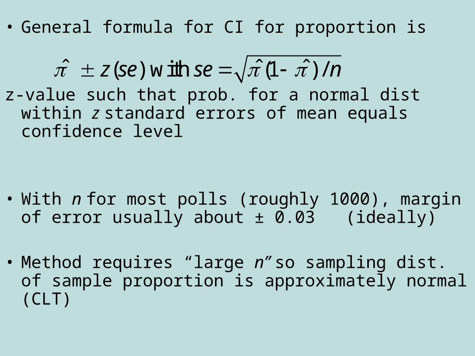
• General formula for CI for proportion is

z-value such that prob. for a normal dist within z standard errors of mean equals confidence level

• With n for most polls (roughly 1000), margin of error usually about ± 0.03 (ideally)

• Method requires “large n” so sampling dist. of sample proportion is approximately normal (CLT)

ˆ ˆ ˆ ( ) with (1 ) /z se se n

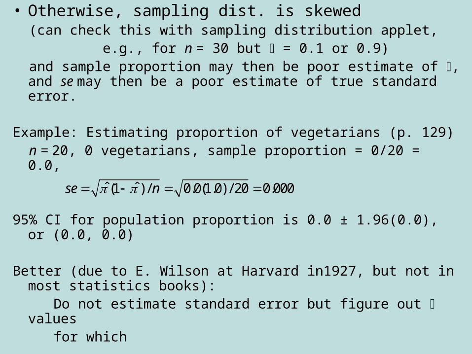
• Otherwise, sampling dist. is skewed (can check this with sampling distribution applet, e.g., for n = 30 but = 0.1 or 0.9) and sample proportion may then be poor estimate of , and se

may then be a poor estimate of true standard error.

Example: Estimating proportion of vegetarians (p. 129) n = 20, 0 vegetarians, sample proportion = 0/20 = 0.0, 95% CI for population proportion is 0.0 ± 1.96(0.0), or (0.0, 0.0)

Better (due to E. Wilson at Harvard in1927, but not in most statistics books):

Do not estimate standard error but figure out values for which

ˆ ˆ(1 ) / 0.0(1.0) / 20 0.000se n

Example: for n = 20 with

solving the quadratic equation this gives for provides solutions 0 and 0.16, so 95% CI is (0, 0.16)

• Agresti and Coull (1998) suggested using ordinary CI (estimate ± z(se)) after adding 2 observations of each type, as a simpler approach that works well even for very small n (95% CI has same midpoint as Wilson CI);

Example: 0 vegetarians, 20 non-veg; change to 2 veg, 22 non-veg, and then we find

95% CI is 0.08 ± 1.96(0.056) = 0.08 ± 0.11, gives (0.0, 0.19).

ˆ| | 1.96 (1 ) / n

ˆ 0,

ˆ 2 / 24 0.083, (0.083)(0.917) / 24 0.056se

Confidence Interval for the Mean

• In large random samples, the sample mean has approx. a normal sampling distribution with mean and standard error

• Thus,

y n

( 1.96 1.96 ) .95y y

P y

• We can be 95% confident that the sample mean lies within 1.96 standard errors of the (unknown) population mean

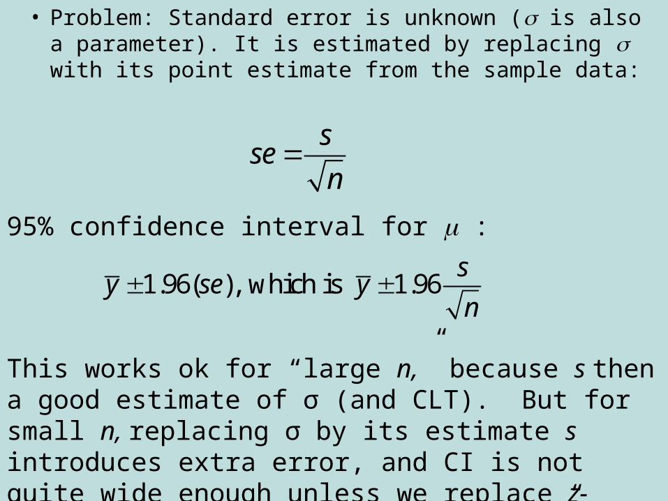
• Problem: Standard error is unknown ( is also a parameter). It is estimated by replacing with its point estimate from the sample data:

sse

n

95% confidence interval for :

This works ok for “large n,” because s then a good estimate of σ (and CLT). But for small n, replacing σ by its estimate s introduces extra error, and CI is not quite wide enough unless we replace z-score by a slightly larger “t-score.”

1.96( ), which is 1.96s

y se yn

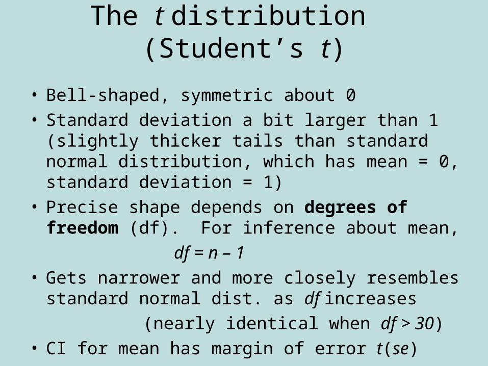
The t distribution (Student’s t)

• Bell-shaped, symmetric about 0• Standard deviation a bit larger than 1 (slightly

thicker tails than standard normal distribution, which has mean = 0, standard deviation = 1)

• Precise shape depends on degrees of freedom (df). For inference about mean,

df = n – 1 • Gets narrower and more closely resembles

standard normal dist. as df increases

(nearly identical when df > 30)• CI for mean has margin of error t(se)

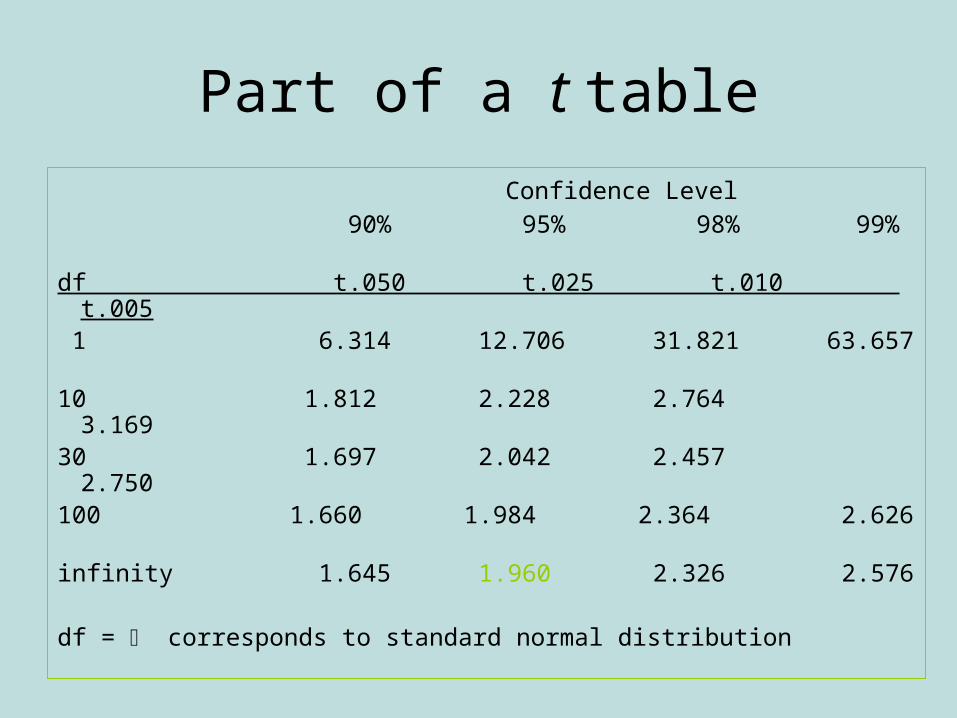
Part of a t table

Confidence Level 90% 95% 98% 99% df t.050 t.025 t.010 t.005 1 6.314 12.706 31.821 63.657 10 1.812 2.228 2.764 3.169 30 1.697 2.042 2.457 2.750 100 1.660 1.984 2.364 2.626 infinity 1.645 1.960 2.326 2.576

df = corresponds to standard normal distribution

CI for a population mean

• For a random sample from a normal population distribution, a 95% CI for µ is

where df = n-1 for the t-score

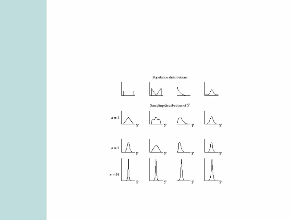
• Normal population assumption ensures sampling distribution has bell shape for any n (Recall figure on p. 93 of text and next page). More about this assumption later.

.025 ( ), with /y t se se s n

Example: Anorexia study (p.120)

• Weight measured before and after period of treatment

• y = weight at end – weight at beginning• Example on p.120 shows results for “cognitive

behavioral” therapy. For n=17 girls receiving “family therapy” (p. 396),

y = 11.4, 11.0, 5.5, 9.4, 13.6, -2.9, -0.1, 7.4, 21.5, -5.3, -3.8, 13.4, 13.1, 9.0, 3.9, 5.7, 10.7

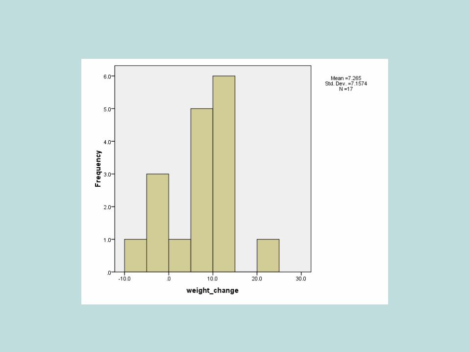
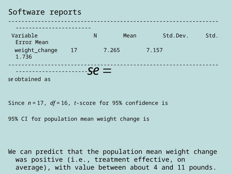
Software reports---------------------------------------------------------------------------------------

Variable N Mean Std.Dev. Std. Error Mean

weight_change 17 7.265 7.157 1.736

----------------------------------------------------------------------------------------

se obtained as

Since n = 17, df = 16, t-score for 95% confidence is

95% CI for population mean weight change is

We can predict that the population mean weight change was positive (i.e., treatment effective, on average), with value between about 4 and 11 pounds.

se

Comments about CI for population mean µ

• Greater confidence requires wider CI• Greater n produces narrower CI• The method is robust to violations of the

assumption of a normal population dist.

(But, be careful if sample data dist is very highly skewed, or if severe outliers. Look at the data.)

• t methods developed by W.S. Gosset (“Student”) of Guinness Breweries, Dublin (1908)

t distribution and standard normal as sampling distributions (normal popul.)

• The standard normal distribution is the sampling distribution of

• The t distribution is the sampling distribution of

( ) ( )

/

y y

se s n

( ) ( )

/y

y y

n

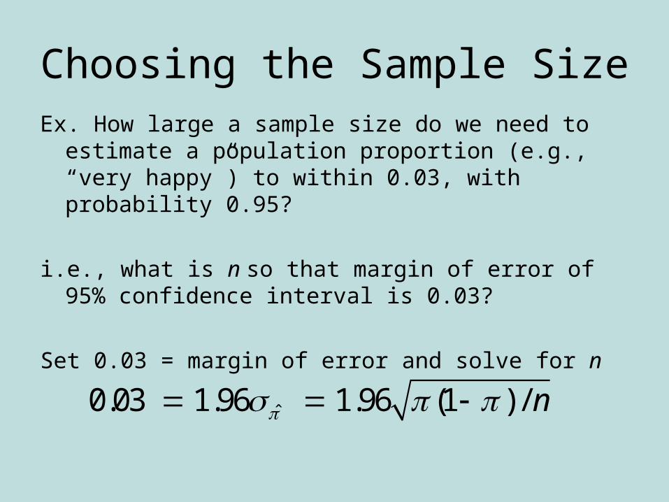
Choosing the Sample SizeEx. How large a sample size do we need to estimate a

population proportion (e.g., “very happy”) to within 0.03, with probability 0.95?

i.e., what is n so that margin of error of 95% confidence interval is 0.03?

Set 0.03 = margin of error and solve for n

ˆ0.03 1.96 1.96 (1 ) / n

Solution

Largest n value occurs for = ???, so we’ll be “safe” by selecting n = .

If only need margin of error 0.06, require

(To double precision, need to quadruple n)

2(1 )(1.96 / 0.03) 4268 (1 )n

2(1 )(1.96 / 0.06) 1067 (1 )n

What if we can make an educated “guess” about proportion value?

• If previous study suggests popul. proportion roughly about 0.20, then to get margin of error 0.03 for 95% CI,

• It’s “easier” to estimate a population proportion as the value gets closer to 0 or 1 (close election difficult)

• Better to use approx value for rather than 0.50 unless you have no idea about its value

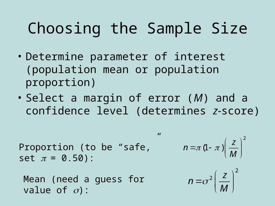
Choosing the Sample Size

• Determine parameter of interest (population mean or population proportion)

• Select a margin of error (M) and a confidence level (determines z-score)

Proportion (to be “safe,” set = 0.50):2

(1 )z

nM

Mean (need a guess for value of ): 2

2 zn

M

Example: n for estimating mean

Future anorexia study: We want n to estimate population mean weight change to within 2 pounds, with probability 0.95.

• Based on past study, guess σ = 7

Note: Don’t worry about memorizing formulas such as for sample size. Formula sheet given on exams.

n

Some comments about CIs and sample size

• We’ve seen that n depends on confidence level (higher confidence requires larger n) and the population variability (more variability requires larger n)

• In practice, determining n not so easy, because (1) many parameters to estimate, (2) resources may be limited and we may need to compromise

• CI’s can be formed for any parameter.

(e.g., see pp. 130-131 for CI for median)

• Confidence interval methods were developed in the 1930s by Jerzy Neyman (U. California, Berkeley) and E. S. Pearson (University College, London)

• The point estimation method mainly used today, developed by Ronald Fisher (UK) in the 1920s, is maximum likelihood. The estimate is the value of the parameter for which the observed data would have had greater chance of occurring than if the parameter equaled any other number.

(picture)

• The bootstrap is a modern method (Brad Efron) for generating CIs without using mathematical methods to derive a sampling distribution that assumes a particular population distribution. It is based on repeatedly taking samples of size n (with replacement) from the sample data distribution.