5 SCIENTIFIC HIGHLIGHT OF THE MONTH

First-principles calculations of the Berry curvature of Bloch

states for charge and spin transport of electrons

M. Gradhand1, D.V. Fedorov2, F. Pientka2,3, P. Zahn2, I. Mertig2,1, and B.L. Gyorffy4

1 - Max-Planck-Institut fur Mikrostrukturphysik, Weinberg 2, D-06120 Halle, Germany

2 - Institut fur Physik, Martin-Luther-Universitat Halle-Wittenberg, D-06099 Halle, Germany

3 - Dahlem Center for Complex Quantum Systems and Fachbereich Physik, Freie Universitat

Berlin, 14195 Berlin, Germany

4 - H.H.Wills Physics Laboratory, University of Bristol, Bristol BS8 1TH, United Kingdom

Abstract

Recent progress in wave packet dynamics based on the insight of M. V. Berry pertaining

to adiabatic evolution of quantum systems has led to the need that a new property of a Bloch

state, the Berry curvature, has to be calculated from first principles. We report here on the

response to this challenge by the ab initio community during the past decade. First we give a

tutorial introduction of the conceptual developments we mentioned above. Then we describe

four methodologies which have been developed for first-principles calculations of the Berry

curvature. Finally, in Section 3, to illustrate the significance of the new developments, we

report some results of calculations of interesting physical properties like anomalous and spin

Hall conductivity.

1 Introduction: Semiclassical electronic transport in solids and

wave packet dynamics with the Berry curvature

Some recent, remarkable advances in the semiclassical description of charge and spin transport

by electrons in solids motivate a revival of interest in a detailed k-point by k-point study of

their band structure. A good summary of the conceptual developments and the experiments

they have stimulated has been given by Di Xiao, Ming-Che Chang and Qian Niu [1]. Here we

wish to review only the role and prospects of first-principles electronic structure calculations in

this rapidly moving field.

1.1 New features of the Boltzmann equation

Classically, particle transport is considered to take place in phase space whose points are la-

beled by the position vector r and the momentum p and described by the distribution function

32

Figure 1: a) The anomalous Hall effect and b) the spin Hall effect.

f(r,p, t) which satisfies the Boltzmann equation. Electrons in solids fit into this framework if

we view the particles as wave packets constructed from the Bloch waves, Ψnk (r) = eik·run(r,k),

eigenfunctions of the crystal Hamiltonian H. If such a wave packet is strongly centered at kc

in the Brillouin zone it predominantly includes Bloch states with quantum numbers k close to

kc and the particle can be said to have a momentum ~ kc. Then, if we call its spatial center rc

its position, the transport of electrons can be described by an ensemble of such quasiparticles.

One of these is described with the distribution function fn(rc,kc, t). For simplicity the band

index n is dropped in the following. As f(rc,kc, t) evolves in phase space the usual form of the

Boltzmann equation, which preserves the total probability, is given by

∂tf +·rc · ∇rcf +

·

kc · ∇kcf =

(δf

δt

)

scatt

. (1)

Here the first term on the left hand side is the derivative with respect to the explicit time

dependence of f , the next two terms account for the time dependence of rc and kc, and the term

on the right hand side is due to scattering of electron states, by defects and other perturbations

in and out of the considered phase space volume centered at rc and kc. The time evolution of

rc (t) and kc (t) is given by semiclassical equations of motion which in the presence of external

electric E and magnetic B fields take conventionally the following form

·rc =

1

~

∂Enk

∂k

∣∣∣∣k=kc

= vn(kc) , (2)

~·

kc = −eE − e·rc × B . (3)

Here, the group velocity vn(kc) involves the unperturbed band structure. In the presence of

a constant electric E = (Ex, 0, 0) and magnetic B = (0, 0, Bz) field the solution of the above

equations yields the Hall resistivity ρxy ∝ Bz. However, for a ferromagnet with magnetization

M = (0, 0,Mz) the above theory can not account for the experimentally observed (additional)

anomalous contribution ρxy ∝ Mz. For a necessary correction of the theory, one needs to

construct a wave packet

Wkc,rc(r,t) =

∑

k

ak(kc, t)Ψnk(r) (4)

carefully taking into account the phase of the weighting function ak(kc, t). Requiring the wave

packet to be centered at rc = 〈Wkc,rc|r|Wkc,rc

〉, it follows that ak(kc, t) = |ak(kc, t)| ei(k−kc)·An(kc),

where

An (kc) = i

∫

u.c.

d3r u∗n(r,kc)∇kun(r,kc) (5)

33

is the Berry connection as will be discussed in detail in the next Section. Note that the integral

is restricted to only one unit cell (u.c.).

Now, using the wave packet of Eq. (4), one can construct the Lagrangian

L(t) = 〈W | i~∂t − H |W 〉 , (6)

and minimize the action functional S[rc(t),kc(t)] =t∫dt′L(t′) with respect to arbitrary variations

in rc(t) and kc(t). This manoeuvre replaces the quantum mechanical expectation values with

respect to Wkc,rc(r,t) by the classical equations of motion for rc(t) and kc(t). From the Euler-

Lagrange equations

∂t∂L

∂·

kc

− ∂L

∂kc= 0 and ∂t

∂L

∂·rc

− ∂L

∂rc= 0 , (7)

one gets

·rc =

1

~

∂Enk

∂k

∣∣∣∣k=kc

−·

kc × Ωn (kc) , (8)

~·

kc = −eE − e·rc × B . (9)

Here Ωn(kc) is the so-called Berry curvature, defined as

Ωn(kc) = ∇k × An(k)|k=kc, (10)

the main subject of this Highlight.

In comparison to Eq. (2), the new equation of motion for rc(t) given by Eq. (8) has an additional

term proportional to the electric field called the anomalous velocity

van(kc) =

e

~E × Ωn (kc) . (11)

The presence of this velocity provides the anomalous contribution to the Hall current jHy =

jH,↑y + jH,↓

y , where the spin-resolved currents may be written as

jH,↑y = −e

∫

BZ

d3kc

(2π)3·ry

c↑(kc)f↑ (kc) = σ↑yx (Mz)Ex . (12)

jH,↓y = −e

∫

BZ

d3kc

(2π)3·ry

c↓(kc)f↓ (kc) = σ↓yx (Mz)Ex . (13)

In that notation f↑ (kc) and f↓ (kc) are the spin-resolved distribution functions which are solu-

tions of Eq. (1). In the limit of no scattering they reduce to the equilibrium distribution functions

and only the intrinsic mechanism governed by the anomalous velocity of Eq. (11) contributes to

the Hall component. In general, jH,↑y and jH,↓

y have opposite sign because of·rc(kc). However,

the resulting charge current is non-vanishing (see Fig. 1 (a)) due to the fact, that the number of

spin-up and spin-down electrons differs in ferromagnets with a finite magnetization M 6= 0. In

contrast to the AHE in ferromagnets, the absence of the magnetization in normal metals leads

to the presence of time inversion symmetry and, as a consequence, jH,↑y = −jH,↓

y . This provides

a vanishing charge current, i.e. Hall voltage, but the existence of a pure spin current as depicted

in Fig. 1 (b), which is known as the spin Hall effect (SHE).

34

1.2 Berry phase, connection and curvature of Bloch electrons

Here we introduce shortly the concept of such relatively novel quantities as the Berry phase,

connection, and curvature which arise in case of an adiabatic evolution of a system.

1.2.1 Adiabatic evolution of eigenstates

Let us consider an eigenvalue problem of the following form

H(r, λ1, λ2, λ3)Φn(r;λ1, λ2, λ3) = En(λ1, λ2, λ3)Φn(r;λ1, λ2, λ3) , (14)

where H is a differential operator, Φn and En are the nth eigenfunction and eigenvalue, re-

spectively, the vector r is a variable, and λ1, λ2, λ3 are parameters restricted for simplic-

ity to the number of three. A mathematical problem of general interest is the way such

eigenfunctions change if the set λ = (λ1, λ2, λ3) changes slowly with time. If it is assumed

that the process is adiabatic, that is to say there is no transition from one to another state,

then for long it was argued that a state Φn(t = 0) evolves in time as Φn(t) = Φn(t = 0)

exp

(− i

~

t∫

0

dt′En(λ1(t′), λ2(t

′), λ3(t′)) + iγn(t)

), where the phase γn(t) is meaningless as it can be

’gauged’ away. In 1984 M. V. Berry [2] has discovered that while this is true for an arbitrary open

path in the parameter space, for a path that returns to the starting values λ1(0), λ2(0), and λ3(0)

the accumulated phase is ’gauge’ invariant and is therefore a meaningful and measurable quan-

tity. In particular, he showed that for a closed path, labeled C in Fig. 2, the phase γn can be

Figure 2: A closed path in the parameter space.

described by a line integral as

γn =

∮

C

dλ ·An(λ) , (15)

where the connection An(λ) is given by

An(λ) = i

∫d3r Φ∗

n(r,λ)∇λΦn(r,λ) . (16)

35

The surprise is that although the connection is not ’gauge’ invariant, γn and even more inter-

estingly the curvature

Ωn(λ) = ∇λ × An(λ) (17)

are. As will be shown presently, these ideas are directly relevant for the dynamics of wave

packets in the transport theory discussed above.

1.2.2 Berry connection and curvature for Bloch states

Somewhat surprisingly the above discussion has a number of interesting things to say about the

wave packets in the semiclassical approach for spin and charge transport of electrons in crystals.

Its relevance becomes evident if we take the Schrodinger equation for the Bloch state

(− ~

2

2m∇

2r + V (r)

)Ψnk(r) = EnkΨnk(r) , (18)

and rewrite it for the periodic part of the Bloch function

(− ~

2

2m(∇r + ik)2 + V (r)

)un(r,k) = Enkun(r,k) . (19)

The point is that the differential equation for Ψnk(r), a simultaneous eigenfunction of the trans-

lation operator and the Hamiltonian, does not depend on the wave vector, since k only labels

the eigenvalues of the translation operator. However, in Eq. (19) k appears as a parameter and

hence the above discussion of the Berry phase, the corresponding connection, and curvature

applies directly. In short, for each band n there is a connection associated with every k given

by

An(k) = i

∫

u.c.

d3r u∗n(r,k)∇kun(r,k) . (20)

Furthermore, the curvature

Ωn(k) = ∇k × An(k) = i

∫

u.c.

d3r∇ku∗n(r,k) × ∇kun(r,k) (21)

is the quantity that appears in the semiclassical equation of motion for the wave packet in

Eq. (8). Thus, the curvature and the corresponding anomalous velocity in Eq. (11) associated

with the band n are properties of un(r,k). To emphasize this point, we note that the Bloch

functions Ψnk(r) are orthogonal to each other

〈Ψnk|Ψn′k′〉 =

∫

crystal

d3r Ψ∗nk(r)Ψn′k′(r) = δk,k′δn,n′ , (22)

and hence k is not a parameter. In contrast, un(r,k) is orthogonal to un′(r,k) but not to

un(r,k′) as this is an eigenfunction of a different Hamiltonian.

The observation that the above connection and curvature are properties of the periodic part

of the Bloch function prompts a further comment. Note, that for vanishing periodic potential

the Bloch functions would reduce to plane waves. Constructing the wave packet from plane

waves means un(r,k) = 1. Evidently, this means that Ωn(k) and An(k) are zero and this fact

is consistent with the general notion that the connection and the curvature arise from including

36

only one or in any case finite number of bands, in constructing the wave packet. The point is that

the neglected bands are the ’outside world’ referred to in the original article of M. V. Berry [2].

In contrast the expansion in terms of plane waves does not neglect any bands since there is just

one band. Thus, the physical origin of the connection and the curvature is due to the periodic

crystal potential breaking up the full spectrum of the parabolic free particle dispersion relation

into bands, usually separated by gaps, and we select states only from a limited number of such

bands to represent the wave packet.

1.3 Abelian and non-Abelian curvatures

So far we have introduced the Berry connection and curvature for a non-degenerate band. In case

of degenerate bands the conventional adiabatic theorem fails. In the semiclassical framework

a correct treatment incorporates a wave packet constructed from the degenerate bands [3, 4].

As a consequence, the Berry curvature must be extended to a tensor definition in analogy to

non-Abelian gauge theories. This extension is originally due to Wilczek and Zee [5].

Let us consider the eigenspace |ui(k〉) : i ∈ Σ of some N -fold degenerate eigenvalue. For

Bloch states the elements of the non-Abelian Berry connection ¯A(k) read

Aij(k) = i 〈ui(k) |∇kuj(k)〉 i, j ∈ Σ , (23)

where Σ = 1, ..., N contains all indices of the degenerate subspace. The definition of the

curvature tensor ¯Ω(k) in a non-Abelian gauge theory has to be extended by substituting the

curl with the covariant derivative as

¯Ω(k) = ∇k × ¯A(k) − i ¯A(k) × ¯A(k) , (24)

Ωij(k) = i

⟨∂ui(k)

∂k

∣∣∣∣×∣∣∣∣∂uj(k)

∂k

⟩+ i∑

l∈Σ

⟨ui(k)

∣∣∣∣∂ul(k)

∂k

⟩×⟨ul(k)

∣∣∣∣∂uj(k)

∂k

⟩.

The subspace of degenerate eigenstates is subject to a U(N) gauge freedom and observables

should be invariant with respect to a gauge transformation of the basis set

∑

i

Uij(k) |ui(k)〉 : i ∈ Σ

with ¯U(k) ∈ U(N). (25)

Consequently, the Berry connection and curvature are transformed according to

¯A′(k) = ¯U †(k) ¯A(k) ¯U(k) + i ¯U †(k)∇k¯U(k) , (26)

¯Ω′(k) = ¯U †(k) ¯Ω(k) ¯U(k). (27)

The curvature is now a covariant tensor and thus not directly observable. However, there are

gauge invariant quantities that may be derived from it. From gauge theories it is known that

the connection and the curvature must lie in the tangent space of the gauge group U(N), i.e.,

the Lie algebra u(N). The above definition of the Lie algebra differs by an unimportant factor

of i from the mathematical convention.

The most prominent example of a non-Abelian Berry curvature appears in materials with time-

reversal (T) and inversion (I) symmetry. For each k point there exist two orthogonal states

|Ψn↑k〉 and |Ψn↓k〉 = TI |Ψn↑k〉 with the same energy, the Kramers doublet. In general, a choice

37

for |Ψn↑k〉 determines the second basis state |Ψn↓k〉 only up to a phase. However, the symmetry

transformation fixes the phase relationship between both basis states. This reduces the gauge

freedom to SU(2) and, consequently, the Berry connection will be an su(2) matrix, which means

its trace vanishes. This is verified easily

〈un↓(k)|∇kun↓(k)〉 = 〈TIun↑(k)|∇kTIun↑(k)〉 = 〈TIun↑(k)|TI ∇kun↑(k)〉 (28)

= −〈un↑(k)|∇kun↑(k)〉 .

For the Kramers doublet the Berry curvature must always be an su(2) matrix because a gauge

transformation induces a unitary transformation of the curvature which does not alter the trace.

The symmetry analysis in the next Section has to be altered since time reversal also changes the

spin TIΩn↑↑(k) = −Ωn↑↑(k) = Ωn↓↓(k), which proves that the trace is indeed zero. Therefore,

in contrast to the spinless case, the Berry curvature may be nontrivial even in nonmagnetic

materials with inversion symmetry.

Despite the Berry curvature being gauge covariant we may derive several observables from it. As

we have seen the trace of the Berry curvature is gauge invariant. In the multiband formulation

of the semiclassical theory, the expectation value of the curvature matrix with respect to the

spinor amplitudes enters the equations of motion [3,4]. In the context of the spin Hall effect one

is interested in Tr( ¯Sj¯Ωi), where ¯Sj is the j-th component of the vector valued su(2) spin matrix.

1.4 Symmetry, Topology, Codimension and the Dirac monopole

It is expedient to exploit symmetries for the evaluation of the Berry curvature. From Eqs. (20)

and (21) we may easily determine the behavior of Ωn(k) under symmetry operations. In crystals

with a center of inversion, the corresponding symmetry operation leaves Enk invariant while r,

r, k, and k change sign, and hence Ωn(k) = Ωn(−k). On the other hand, when time-reversal

symmetry is present Enk, r, and k remain unchanged while r and k are inverted, which leads

to an antisymmetric Berry curvature Ωn(k) = −Ωn(−k). Thus, if time-reversal and inversion

symmetry are present simultaneously the Berry curvature vanishes identically. This is true

in spinless materials only. Taking into account spin we have to acknowledge the presence of

a twofold degeneracy of all bands throughout the Brillouin zone [6, 7], the Kramers doublet,

discussed in the previous Section.

As was mentioned already in Section 1.2.2, the Berry curvature of a band arises due to the

projection onto this band, e.g., in the semiclassical one band theory it keeps an information

about the influence of other adjacent bands. If a band is well separated from all other bands

by an energy scale large compared to one set by the time scale of the adiabatic evolution, the

influence of the other bands is negligible. In contrast, degeneracies of energy bands deserve

special attention, since the conventional adiabatic theorem fails there. Special attention has

been paid to pointlike degeneracies, where the intersection of two energy bands is shaped like a

double cone or a diabolo (Fig. 3, left). These degeneracies are called diabolical points [8].

According to M. V. Berry [2] we can linearize the Hamiltonian near such a point and rewrite it

as an effective two band Hamiltonian

H(r) =

(z x− iy

x+ iy −z

)

= riσi , (29)

38

Figure 3: Left: Conical intersection of energy surfaces. Right: Direction of the Monopole field.

where σi are the Pauli matrices and the r space is some suitable parametrization of the Brillouin

zone. The eigenvalues are ±|r|, hence the dispersion is shaped like a cone. The degeneracy lies

at the origin of the r parameter space and the curvature is given by

Ω±(r) = ±1

2

r

r3. (30)

This is precisely the form of the monopole of a magnetic field with a charge 1/2 (Fig. 3, right).

Diabolical points always have this charge, while nonlinear intersections may have higher charges

[10]. In general, the monopole charge is a topological invariant and quantized to integer multiples

of 1/2. This is a consequence of the quantization of the Dirac monopole [9].

In more general language, the Berry curvature flux through a closed two-dimensional manifold

∂M is the first Chern number Cn of that manifold and thus an integer. Since the (Abelian)

curvature is defined as the curl of the connection it must be divergence free except for the

monopoles. We can then exploit Gauss’ theorem

Cn =1

2π

∫

∂MdσΩnn =

1

2π

∫

Md3r ∇ · Ωn = m , m ∈ N . (31)

Here n is the normal vector of the surface element. If we assume that each monopole contributes a

Chern number of ±1 the above equation implies for the Berry curvature ∇·Ω = 4π∑

j gjδ(r−rj),

where gj = ±1/2. The solution of this differential equation yields the source term of the Berry

curvature

Ω(r) =∑

j

gjr − rj

|r − rj|3+ ∇ ×A(r) , (32)

which proves that there are monopoles with a charge quantized to 1/2 times an integer.

The mathematical interpretation of the Berry curvature in terms of the theory of fiber bundles

and Chern classes and the connection to the theory of the quantum Hall effect, where the Chern

number appears as the Thouless-Kohmoto-Nightingale-den Nijs (TKNN) integer [11] has been

first noticed by Simon [12].

However, monopoles are not only interesting in a mathematical sense but also for actual calcu-

lations of quantities such as the anomalous Hall conductivity. On the one hand, singularities

of the Berry curvature near the Fermi surface greatly influence the numerical stability of the

39

result. On the other hand, Haldane [13] has pointed out that the Chern number and thus the

anomalous Hall conductivity can be changed by creation and annihilation of Berry curvature

monopoles.

To identify monopoles in a parameter space one is interested in degeneracies that do not occur

on account of any symmetry and have thus been called accidental. For a single Hamiltonian

without symmetries the occurrence of degeneracies in the discrete spectrum is infinitely unlikely.

For Hamiltonians that depend on a set of parameters one can ask how many parameters are

needed in order to encounter a twofold degenerate eigenvalue. This number is called codimen-

sion. According to a theorem by von Neumann and Wigner [14], for a generic Hamiltonian the

answer is three. In other words, degeneracies are points in a three-dimensional parameter space

like the Brillouin zone. For this reason accidental degeneracies are diabolical points.

If the Hamiltonian is real, which is equivalent to being invariant with respect to time reversal,

the number of parameters we have to vary reduces to two [15]. However, we have seen that in

the case of nonmagnetic crystals with inversion symmetry each band is twofold degenerate. This

degeneracy arises due to a symmetry and is not accidental. The theorem of von Neumann and

Wigner does not apply. As a consequence, accidental degeneracies of two different bands would

have to be fourfold. In this case the codimension is five and the occurrence of an accidental

degeneracy is infinitely unlikely in the Brillouin zone.

This is the reason why we only observe avoided crossings for nonmagnetic crystals with inver-

sion symmetry, since and all accidental crossings are lifted by spin-orbit coupling. In order to

encounter accidental two-fold degeneracies of codimension two, we would, thus, need to consider

a nonmagnetic band structure without inversion symmetry of the lattice.

1.5 The spin polarization gauge

As was discussed in the previous Sections, in spinless crystals with time-reversal and inversion

symmetry the Berry curvature vanishes at every k point [16]. If spin degrees of freedom are

taken into account the band structure is twofold degenerate throughout the Brillouin zone due

to Kramers degeneracy plus inversion symmetry and consequently the Berry curvature is rep-

resented by an element of the Lie algebra su(2). In contrast to the scalar case, this matrix is

gauge covariant and hence not observable. In order to gain some insight to the Berry curvature

of nonmagnetic materials we would like to visualize it. To this end we must be able to compare

the Berry curvature at different points in k space, thus we have to choose a universal gauge.

Then we can plot the first diagonal element of the su(2) matrix which should be continuous in

such a gauge.

One natural choice of a gauge (let us call it gauge I) is to ensure that the spin polarization of

one Kramers state is always parallel to the z direction and positive [17] that is

〈Ψ↑k|σx|Ψ↑k〉 = 0

〈Ψ↑k|σy|Ψ↑k〉 = 0

〈Ψ↑k|σz|Ψ↑k〉 > 0

. (33)

This means for the second Kramers state

〈Ψ↓k|σz|Ψ↓k〉 = −〈Ψ↑k|σz|ψ↑k〉 < 0. (34)

40

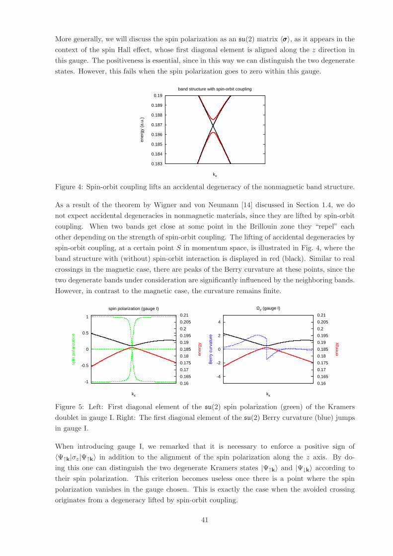
More generally, we will discuss the spin polarization as an su(2) matrix 〈σσσ〉, as it appears in the

context of the spin Hall effect, whose first diagonal element is aligned along the z direction in

this gauge. The positiveness is essential, since in this way we can distinguish the two degenerate

states. However, this fails when the spin polarization goes to zero within this gauge.

0.183

0.184

0.185

0.186

0.187

0.188

0.189

0.19

ener

gy (

a.u.

)

kx

band structure with spin-orbit coupling

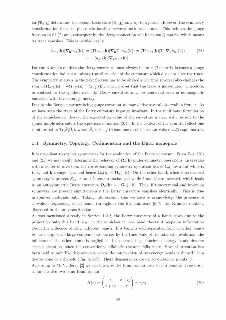
Figure 4: Spin-orbit coupling lifts an accidental degeneracy of the nonmagnetic band structure.

As a result of the theorem by Wigner and von Neumann [14] discussed in Section 1.4, we do

not expect accidental degeneracies in nonmagnetic materials, since they are lifted by spin-orbit

coupling. When two bands get close at some point in the Brillouin zone they “repel” each

other depending on the strength of spin-orbit coupling. The lifting of accidental degeneracies by

spin-orbit coupling, at a certain point S in momentum space, is illustrated in Fig. 4, where the

band structure with (without) spin-orbit interaction is displayed in red (black). Similar to real

crossings in the magnetic case, there are peaks of the Berry curvature at these points, since the

two degenerate bands under consideration are significantly influenced by the neighboring bands.

However, in contrast to the magnetic case, the curvature remains finite.

-1

-0.5

0

0.5

1

0.16

0.165

0.17

0.175

0.18

0.185

0.19

0.195

0.2

0.205

0.21

spin

pol

ariz

atio

n

ener

gy

kx

spin polarization (gauge I)

-4

-2

0

2

4

0.16

0.165

0.17

0.175

0.18

0.185

0.19

0.195

0.2

0.205

0.21

Ber

ry c

urva

ture

ener

gy

kx

Ωz (gauge I)

Figure 5: Left: First diagonal element of the su(2) spin polarization (green) of the Kramers

doublet in gauge I. Right: The first diagonal element of the su(2) Berry curvature (blue) jumps

in gauge I.

When introducing gauge I, we remarked that it is necessary to enforce a positive sign of

〈Ψ↑k|σz|Ψ↑k〉 in addition to the alignment of the spin polarization along the z axis. By do-

ing this one can distinguish the two degenerate Kramers states |Ψ↑k〉 and |Ψ↓k〉 according to

their spin polarization. This criterion becomes useless once there is a point where the spin

polarization vanishes in the gauge chosen. This is exactly the case when the avoided crossing

originates from a degeneracy lifted by spin-orbit coupling.

41

This situation is illustrated in Fig. 5, where the spin polarization for both Kramers states of the

lower doublet is shown. The spin polarization becomes zero at the avoided crossing. In fact,

the picture suggests that the spin polarizations of both states change sign, which means that

by enforcing gauge I we have changed from the first to the second Kramers state while crossing

point S. Indeed, this is verified by the graph of the first diagonal element of the Berry curvature

in this gauge presented in Fig. 5. Exactly at the point where the spin polarization vanishes, the

Berry curvature changes sign, jumping from one degenerate state to the other. This jumping

is unsatisfactory, since it does not allow us to plot the Berry curvature consistently throughout

the BZ without adjustment by hand. A way out is provided by a different gauge [18,19].

This new gauge (let us call it gauge II) describes the nonmagnetic crystal as the limit of vanish-

ing exchange splitting in a magnetic crystal. The task is then to find the unitary transformation

that diagonalizes the perturbation operator Hxc in the degenerate subspace of the Kramers

doublet. This amounts to the condition

〈Ψ↑k|Hxc|Ψ↓k〉 ∼ 〈Ψ↑k|σz|Ψ↓k〉 = 0, (35)

where Ψ↑↓k denote the two Kramers states. The above equation accounts for the two free

parameters we have to fix. Furthermore, we choose the sign as

〈Ψ↑k|σz|Ψ↑k〉 > 0. (36)

In gauge II the diagonal elements of the nonmagnetic spin polarization represents the analytical

continuation of the magnetic spin polarizations with vanishing exchange splitting.

-1

-0.5

0

0.5

1

0.16

0.165

0.17

0.175

0.18

0.185

0.19

0.195

0.2

0.205

0.21

spin

pol

ariz

atio

n

ener

gy

kx

spin polarization (gauge II)

-30

-20

-10

0

10

20

30

0.16

0.165

0.17

0.175

0.18

0.185

0.19

0.195

0.2

0.205

0.21

Ber

ry c

urva

ture

ener

gy

kx

Ωz (gauge II)

Figure 6: Left: Nonmagnetic spin polarization (green) of the lower doublet in gauge II. Right:

The first diagonal element of the su(2) Berry curvature (blue) remaining continuous in gauge II.

In Fig. 6 the same avoided crossing as in Fig. 5 is shown while gauge II has been imposed.

The spin polarization now remains finite and the Berry curvature is continuous, thus we have

resolved the ambiguity.

42

2 First principle calculations of the Berry curvature for Bloch

Electrons

2.1 KKR method

In this Section we describe the most recent of four methods developed for calculating the Berry

curvature. This approach [20] is based on the screened version of the venerable KKR method [21]

and is motivated by the fact that in the multiple scattering theory the wave vector k enters the

problem only through the structure constants GsQQ′(E ;k), defined in Eq. (40). Those depend on

the geometrical arrangement of the scatterers but not on the scattering potentials at the lattice

sites. Hence the sort of k derivatives that occur in the definition of the connection in Eq. (20)

should involve only the derivative ∇kGsQQ′(E ;k) easy to calculate within the screened KKR

method. In what follows we demonstrate that such expectation can indeed be realized and an

efficient algorithm is readily constructed which takes full advantage of these features.

As it is clear from Eqs. (20) and (21), the connection An(k) and the curvature Ωn(k) are

the properties of the periodic component un(r,k) of the Bloch state Ψnk(r). However, as in

most band theory methods, in the KKR one calculates the Bloch wave. Thus, to facilitate the

calculation of An(k) and Ωn(k) from Ψnk(r) one must recast the problem. A useful way to

proceed with it is to rewrite

An(k) = i

∫

u.c.

d3r u†n(r,k)∇kun(r,k)

= i

∫

u.c.

d3r Ψ∗nk(r)∇kΨnk(r) +

∫

u.c.

d3r Ψ∗nk(r)rΨnk(r) , (37)

where the integrals are over the unit cell.

Since the most interesting physical consequences of the Berry curvature occur in spin-orbit

coupled systems, the theory is developed in terms of a fully relativistic multiple scattering

theory based on the Dirac equation. In short, the four component Dirac Bloch wave [22] is

expanded around one site in terms of the local scattering solutions ΦQ(E ; r) of the radial Dirac

equation as [20]

Ψnk(r) =∑QCn,Q(k)ΦQ(E ; r) . (38)

In such a representation the expansion coefficients Cn,Q(k) are solutions of the eigenvalue prob-

lem¯M(E ;k)Cn(k) = λnCn(k) with Cn(k) = Cn,Q(k) (39)

for the KKR matrix [20]

MQQ′(E ;k) = GsQQ′(E ;k)∆tsQ′(E) − δQQ′ , (40)

where GsQQ′(E ;k) are the relativistic screened structure constants, ∆tsQ′(E) is the ∆t matrix of

the reference system [21] and the eigenvalues λn (E ,k) vanish for E = Enk.

Note, that the eigenvalue problem Eq. (39) depends parametrically on k. Therefore, one can

formally deploy the original arguments of M. V. Berry [2] to derive an expression for the curvature

43

associated with this problem. Namely, one finds (here for the sake of simplicity we assume the

matrix ¯M to be Hermitian) [20]

ΩKKRn (k) = −Im ∑

m6=n

C†n∇k

¯MCm×C†m∇k

¯MCn

(λn−λm)2 . (41)

Evidently, this curvature is the property of the KKR matrix ¯M(E ;k). What is important about

this result is the fact that the k derivative operates only on ¯M(E ;k) and therefore it can be

expressed simply by

∂ ¯Gs(E ;k)/∂k = i∑R

ReikR ¯Gs(E ;R) , (42)

due to the feature of the screened structure constants. This formula can be easily evaluated since

the screened real space structure constants ¯Gs(E ;R) are short ranged. While this is reassuringly

consistent with the expectation at the beginning of this Section this is not the whole story. The

curvature of the KKR matrix is not that of the Hamiltonian

Hk(r) = e−ik·rH(r)eik·r (43)

whose eigenfunctions are the periodic components un(r,k). In fact, when we evaluate Eq. (37)

we find

An(k) = Akn(k) + Ar

n(k) = AKKRn (k) + Av

n(k) + Arn(k) . (44)

Here we have the KKR part

AKKRn (k) = iC†

n∇kCn = −ImC†n∇kCn , (45)

Avn(k) = ivnC

†n

¯∆Cn = −vnImC†n

¯∆Cn , (46)

with

( ¯∆)QQ′(E) = δQQ′

∫

u.c.d3r Φ†

Q(E ; r)∂ΦQ′ (E;r)

∂E , (47)

and the dipole part

Arn(k) = C†

n(k)¯rCn(k) , (48)

with the matrix elements of the position operator

(¯r)QQ′(E) =∫

u.c.d3r Φ†

Q(E ; r)rΦQ′(E ; r) . (49)

As will be shown, the contribution from the first term of r.h.s of Eq. (44) provides the curvature

associated with the KKR matrix in Eq. (41), while the velocity term Avn(k) and dipole term

Arn(k) lead to small corrections.

2.1.1 KKR formula for the Abelian Berry curvature

Starting from the Berry connection introduced above it is straightforward to extend the method

to the Berry curvature expressions. For the Abelian case the Berry curvature is given by three

contributions

Ωn(k) = ∇k × An(k) = Ωkn(k) + Ωr

n(k) = ΩKKRn (k) + Ωv

n(k) + Ωrn(k) , (50)

44

stemming from the analogue terms in Eq. (44). Here, the KKR part which is shown to be the

dominant contribution [20] takes the simple form

ΩKKRn (k) = i∇kC

†n × ∇kCn = −Im∇kC

†n × ∇kCn , (51)

where just the expansion coefficients are involved. Now, an important step is to shift the k

derivative towards the k-dependent KKR matrix. Actually, because of the chosen KKR-basis

set in Eq. (38), one has to deal with a non-Hermitian KKR matrix. However, in order to simplify

the further discussion and to have a clear insight into the presented approach, here the matrix ¯M

is assumed to be Hermitian. Then, introducing a complete set of eigenvectors of the KKR matrix

leads to Eq. (41) which is quite similar to one obtained in the original paper of M. V. Berry.

The difference is just that the k-dependent Hamiltonian is replaced by the k-dependent KKR

matrix of finite dimension. As was already discussed, the partial k derivative of the KKR matrix

can be calculated analytically within the screened KKR method. In a similar way the velocity

and the dipole terms can be treated. Both contributions are typically one order of magnitude

smaller than the KKR part [20]. Moreover, the velocity part of the Berry curvature is always

strictly perpendicular to the group velocity. This fact is a technically very important feature

since for a Fermi surface integral over the Berry curvature this contribution would identically

vanish.

2.1.2 KKR formula for non-Abelian Berry curvature

For a treatment of the non-Abelian Berry curvature not only the conventional connection has

to be taken into account, but also the commutator, which is provided by the requirement of the

gauge invariant theory, has to be considered. As a consequence, the Berry curvature is defined

as

Ωij(k) = i 〈∇kui (k) | × |∇kuj (k)〉 − i∑

l∈Σ

〈∇kui (k) |ul (k)〉 × 〈ul (k) |∇kuj (k)〉 . (52)

Here, as was discussed in section 1.3, Σ contains all indices of the degenerate subspace. Rewriting

it in terms of the Bloch states yields

Ωij(k) = i 〈∇kΨik| × |∇kΨjk〉 + 〈∇kΨik × r|Ψjk〉 − 〈Ψik|r× ∇kΨjk〉−

− ∑l∈Σ

i 〈∇kΨik|Ψlk〉 × 〈Ψlk|∇kΨjk〉− 〈Ψik|r|Ψlk〉 × 〈Ψlk|∇kΨjk〉+

+ 〈∇kΨik|Ψlk〉 × 〈Ψlk|r|Ψjk〉 + i 〈Ψik|r|Ψlk〉 × 〈Ψlk|r|Ψjk〉 ,

(53)

and a similar decomposition into the KKR, velocity and dipole parts

Ωij(k) = ΩKKRij (k) + Ωv

ij(k) + Ωrij(k) (54)

can be performed.

In Fig. 7 the absolute value of the diagonal component of the non-Abelian (vector-valued matrix)

Berry curvature over the Fermi surface of several metals is shown. An evident anisotropy of

the distribution with the values enhanced in z direction is caused by the choice of the gauge

45

Figure 7: The absolute value (in a.u.) of the diagonal component of the non-Abelian Berry cur-

vature |Ωzii(k)| for the Fermi surface of several metals. From left to right Al (3rd and 5th band),

Cu (11th band), Au (11th band) and Pt (9th and 11th band). For Al we used a logarithmic

scale to visualize the important regions [20].

transformation, namely the requirement for the off-diagonal matrix elements of the spin operator

Σz = βσz in the subspace of the two degenerate bands to be zero (see the discussion in Section

1.5). In addition, near degeneracies at the Fermi level lead to enhanced Berry curvatures as

can be seen for Al and Pt. Furthermore, the energy resolved Berry curvature (here S(E) is the

isosurface of constant energy E in the k space)

Ωz(E) =∑

n

∫

S(E)

d2k

|vn(k)|Ωz,+n (k) (55)

is shown in Fig. 8. It proves that the KKR part of Eq. 54 is the dominant contribution to the

Berry curvature. Clearly visible is the quite spiky structure of the curvature as a function of

the energy. As discussed in the literature, this makes the integration of the Berry curvature

computationally demanding, requiring a large number of k and energy points.

-10.0 -8.0 -6.0 -4.0 -2.0 0.0

-60

-40

-20

0

20

40

60

80

100

-3

-2

-1

0

1

2

3

4

5

z (

) a.

u.

E [eV]

KKR part dipole part

Figure 8: The energy resolved Berry curvature Ωz(E) for Au divided into the parts ΩKKR(E)

and Ωr(E) according to Eq. 54 and [20].

2.2 Tight-Binding Model

The tight-binding model provides a convenient framework for studying the geometric quantities

in band theory. We will briefly introduce the tight-binding method with spin-orbit coupling and

46

exchange interaction. The usefulness of this model is then illustrated by discussing interesting

features of the Berry curvature of a simple band structure.

The tight-binding model assumes that the electronic wave function at each lattice site is well

localized around the position of the atom. For this purpose one assumes the crystal potential

to consist of a sum of spherically symmetric, somewhat strongly attractive potentials located

at the core positions. The idea is to treat the overlap matrix elements as a perturbation and

consequently expand the wave function in a basis of atomic orbitals φα(r− Ri). The ansatz

Ψnk(r) =1√N

∑

Ri

eikRi

∑

α

Cnα(k)φα(r − Ri) (56)

ensures that Ψnk fulfills the Bloch theorem. The simplest case involves neglecting the overlap

matrix elements of the wave function

〈φβ(r − Rj) |φα(r − Ri)〉 ∼ δα,βδRi,Rj. (57)

The normalized eigenfunctions in on-site approximation are subject to the eigenvalue problem

〈Ψnk|H|Ψnk〉 = Enk. The solution to this problem in the tight-binding formulation of Eq. (56)

requires the diagonalization of the tight-binding matrix

Hαβ =∑

Ri,Rj

eik(Ri−Rj) 〈φα(r− Rj)|H|φβ(r − Ri)〉 . (58)

Then the coefficients Cnα are obtained as the components of the eigenvector of this matrix and

thus the eigenstates necessary for the evaluation of the Berry curvature are easily accessible.

The matrix elements in Eq. (58) can be parametrized by the method of Slater and Koster [23].

In order to observe a nontrivial Berry curvature we need to take into account spin degrees of

freedom. This doubles the number of bands compared to the spinless case. Within the scope of

the tight-binding model the spin-orbit interaction is treated as a perturbation

VSOC =~

4m2c2(∇rV (r) × p)S = VSOC =

2λ

~2LS (59)

to the Hamiltonian. Here a spherical symmetric potential is assumed and the parameter λ is

considered to be small with respect to the on-site and hopping energies. The matrix elements of

this operator have been listed elsewhere for basis states of p, d and f symmetry [24] in on-site

approximation, although the formalism presented here does not require this approximation.

Furthermore, one can use this model to describe a ferromagnetic material by incorporating an

exchange interaction term. The simplest formulation originates from the mean field theory.

Without taking into account any temperature dependence, a constant exchange field is assumed

and the z axis is chosen as the quantization direction

Hxc = −Vxcσσσ = −Vxcσz , (60)

where Vxc is a positive real number.

2.2.1 Berry Curvature in the Tight-Binding Model

As in the case of the KKR method discussed in the previous Section, solving the eigenproblem

of the tight-binding matrix gives the Bloch wave |Ψnk〉 instead of the periodic function |un(k)〉.

47

Hence, one also needs to consider the two parts, Ωk (k) and Ωr (k), of the Berry curvature

introduced by Eq. (50). Exploiting the on-site approximation of Eq. (57) and the normalization

condition for the coefficents, one gets the first term for the Abelian case in a well known form

Ωkn(k) = i 〈∇kΨnk | × |∇kΨnk〉u.c. = i∇kC

†n(k) × ∇kCn(k)

= −Im∑

m6=n

C†n(k)∇k

¯H(k)Cm(k) × C†m(k)∇k

¯H(k)Cn(k)

(En − Em)2. (61)

The second, dipole, term is given by

Ωrn(k) = ∇k × 〈Ψnk | r |Ψnk〉cell = ∇k ×

(C

†n(k)¯rCn(k)

)

=∑

m6=n

2Re

[C

†n(k)∇k

¯H(k)Cm(k)

En − Em×(C

†m(k)¯rCn(k)

)], (62)

where we have introduced the vector valued matrix ¯r with the components rαβ = 〈φβ(r) | r |φα(r)〉.Similar to the screened KKR method, the k derivative of ¯H(k) in the equations above may be

performed analytically and no numerical derivative is needed.

In the case of degenerate bands, the non-Abelian Berry curvature Ωij(k) = Ωkij(k) + Ωr

ij(k) is

expressed in the following terms (according to Section 1.3, Σ contains all indices of the degenerate

subspace)

Ωkij =i

∑

m/∈Σ

C†i (k)∇k

¯H(k)Cm(k) × C†m(k)∇k

¯H(k)Cj(k)

(Ei − Em) (Ej − Em), (63)

Ωrij =

∑

m/∈Σ

[

−(C

†i (k)¯rCm(k)

)× C

†m(k)∇k

¯H(k)Cj(k)

Ej − Em(64)

+C

†i (k)∇k

¯H(k)Cm(k)

Ei − Em×(C

†m(k)¯rCj(k)

)]

− i∑

l∈Σ

(C

†i (k)¯rC l(k)

)×(C

†l (k)¯rCj(k)

).

Here only the last term is not a direct generalization of the Abelian Berry curvature. Again it

is possible to circumvent the numerical derivative by a summation over all states that do not

belong to the degenerate subspace. The last term does not involve any derivative, therefore the

sum runs only over the degenerate bands.

2.2.2 Diabolical Points

To illustrate the behavior of the Berry curvature near degeneracies, we present calculations of

a simple band structure using the tight-binding method. We consider a ferromagnetic simple

cubic crystal with eight bands including one band with s symmetry and three bands with p

symmetry for each spin direction. Due to the exchange interaction there is no time-reversal

symmetry and the codimension of degeneracies is three.

Regions of the parameter space with a higher symmetry (e.g., high symmetry lines in the Bril-

louin zone) are more likely to support accidental degeneracies because the symmetry possibly

reduces the codimension only in this region. Level crossings on a high symmetry line in the

48

0.16

0.162

0.164

0.166

0.168

0.17

0.172

0.174

0.176

0.178

0.18

π/4π/8 0

ener

gy (

a.u.

)

kx

band structure in (001) direction

P

Figure 9: Left: The crossing of some p bands of a ferromagnetic simple cubic band structure

near the center of the Brillouin zone. Right: Conical intersection of energy surfaces. The z axis

represents the energy dispersion of two intersecting bands over an arbitrary plane in k space

through the diabolical point. The color scale denotes the spin polarization corresponding to

each band.

Brillouin zone do not necessarily occur on account of symmetry as long as the bands are not

degenerate at points nearby which have the same symmetry.

As an example, in Fig. 9 a few bands of the band structure near the Γ point along a high

symmetry line are plotted. There occur three crossings between different bands. On the right-

hand side, the energy dispersion in a plane through the degeneracy is displayed in order to show

the cone shape of the intersection. The color scale represents the spin polarization 〈Ψ|σz|Ψ〉 of

the corresponding band. Within one band the spin polarization rapidly changes in the vicinity

of the degeneracy. At the degeneracy itself it jumps due to the cusp of the corresponding band.

However, when passing the intersection along a straight line in k space and jumping from the

lower to the upper band apparently the spin polarization does not change at all. This is a clear

indication that the character of the two bands is exchanged at the intersection.

The behavior of the spin polarization near the diabolical point illustrates how observables are

influenced by other bands nearby. The Berry curvature can be viewed as a measure of this

coupling which becomes evident from Eqs. (61) and (62), where a sum over all other bands is

performed weighted by the inverse energy difference. M. V. Berry has called this in a more

general context the coupling to the “rest of the universe” [2]. Hence, the Berry curvature of a

single Bloch band generally arises due to a projection onto this band and it becomes large when

other bands are close. As we have seen before, a degeneracy produces a singularity of the Berry

curvature and the adiabatic single-band approximation fails.

In our case the origin of the Berry curvature is the spin-orbit coupling. Since degenerate or

almost degenerate points in the band structure produce large spin mixing of the involved bands,

a peak in the Berry curvature can also be understood from this point of view.

As discussed in Section 1.4, we would expect the curvature around the degeneracy to obey the

1/|k − k0|2-law of a Coulomb field. The asymptotic, spherically symmetric behavior becomes

evident when plotting 1/√

|Ω| in some plane the degeneracy lies in (see Fig. 10). We observe

an absolute value function |k − k0|, which proves that the Berry curvature really has the form

of the monopole field strength given by Eq. (30).

Besides the absolute value we can also examine the direction of the Berry curvature vector. In

49

Fig. 11, we recognize the characteristic monopole field. In the lower band the monopole is a

source, in the upper band a drain of the Berry curvature. This has been expected because a

monopole in one band has to be matched by a monopole of opposite charge in the other band

involved in the degeneracy.

In general, we may assign a “charge” g to the monopole as in Eq. (30). This charge is quantized

to be either integer or half integer. In order to determine the charge numerically one could

perform a fit of the numerical data with the monopole field strength. However there is no

reason to believe that all directions in k space must be equivalent. Some distortion in a certain

direction might result in ellipsoidal isosurfaces of |Ω| instead of spherical ones. A different

approach, independent from the coordinate system exploits Eq. (31)∫

Vd3k∇ ·Ω =

∫

∂Vdsn ·Ω = 2πm m ∈ Z, (65)

where n is a normal vector on the bounding surface ∂V of some arbritray volume V . Performing

the numerical surface integration causes no problem since the Berry curvature is analytical on

the surface unlike at the degeneracy.

So as to validate this formula, the total monopole charge in a sphere of radius r centered at a

generic point in the Brillouin zone near P (see Fig. 9) is evaluated. This flux divided by 2π as

a function of the sphere’s radius is plotted in Fig. 12.

The integral is observed to be quantized to integer multiples of 2π. When increasing the radius

of the sphere the surface crosses various diabolical points. Each time this happens the flux

jumps by ±2π depending on whether the charge of the Berry curvature monopole is positive

or negative. According to Eq. (65), this confirms that the charges of the monopoles created by

the point-like degeneracies are g = ±1/2. Altogether there are six jumps, which means there

are six diabolical points in the vicinity of the point P (see Fig. 9). Two of the monopoles in

the upper band have a negative, the other four a positive charge of 1/2. A generic point as the

center of the integration sphere is chosen to avoid crossing more than one diabolical point at the

time. The deviations from a perfect step function are due to the discretization of the integral,

which increases the error when the surface crosses a monopole. The step functions also verify

the statement that monopoles are the only possible sources of the Berry curvature.

F. D. M. Haldane [13] describes the dynamics of these degeneracies with respect to the variation

of some control parameter, including the creation of a pair of diabolical points and their re-

0 0.001 0.002 0.003 0.004 0.005 0.006 0.007 0.008 0.009 0.01

-0.005

0

0.005

0.01 0.617

0.622

0.627

0.632 0

0.002

0.004

0.006

0.008

0.01

1/| Ω| 2 for the upper band around P

kx kz

Figure 10: Left: Absolute value of the Berry curvature |Ω| plotted over a plane in k space.

Right: Inverse square root of the absolut value, i.e., 1/√

|Ω|.

50

0.615

0.62

0.625

0.63

0.635

-0.01 -0.005 0 0.005 0.01

k z

kx

Ω/| Ω| for the lower band

0.616

0.618

0.62

0.622

0.624

0.626

0.628

0.63

0.632

0.634

-0.008 -0.006 -0.004 -0.002 0 0.002 0.004 0.006 0.008 0.01

k z

kx

Ω/| Ω| for the upper band

Figure 11: Normalized Berry curvature vector around P (see Fig. 9).

-1.5

-1

-0.5

0

0.5

1

1.5

2

2.5

0 0.1 0.2 0.3 0.4 0.5 0.6

flux/

(2π)

radius

Berry curvature flux through spherical surface

Figure 12: The value of the integral Eq. (65) over a spherical surface for the upper band is

plotted against the radius of the sphere.

combination after relative displacement of a reciprocal lattice vector. In the considered case an

obvious choice for the control parameters would be λ or Vxc, regulating the strength of spin-orbit

coupling or exchange splitting, respectively.

Thus, the tight-binding code provides an excellent tool for an investigation of the effects con-

nected with the accidental degeneracy of bands (see for instance, Ref. [13]) since one may scan

through a whole range of parameters without consuming much computational resources and still

obtain qualitatively reliable results.

2.3 Wannier Interpolation scheme

The first method developed specifically for calculating the Berry curvature of Bloch electrons

using the full machinery of the Density Functional Theory (DFT) was based on the Wannier

interpolation code of Marzari, Souza and Vanderbilt [25]. As in the case of the KKR method

presented in Section 2.1 the essence of this approach by Wang et al. [19] is that it avoids taking

the derivative of the periodic part of the Bloch function un(r,k) with respect to k numerically by

finite differences. A second almost equally important feature is that it offers various opportunities

51

to interpolate between different k points in the Brillouin zone and hence reducing the number

of points at which full ab initio calculations need to be performed.

Note that the formulas, naturally arising in wave packet dynamics, for the Berry connection

and curvature, given by Eqs. (20) and (21), involve the real space integrals over a unit cell only.

Extending them to cover all space by using the Wannier functions defined as

|R,n〉 =Vu.c.

(2π)3

∫

BZ

d3k e−ik·R |Ψk,n〉 ,

the Bloch theorem and some care with the algebra one finds the following remarkably simple

results [19,26]

An(k) =∑

R

〈0n| r |R,n〉 eik·R and Ωn(k) = i∑

R

〈0n|R× r |R,n〉 eik·R , (66)

where the matrix elements with respect to the Wannier states, as usual, involve integrals over

all space. These formulas turn up and play a central role in the method of Wang et al. [19] and

make the Wannier interpolation approach looking different from that based on the KKR method

which makes use of expansions and integration within a single unit cell only. The lattice sums

in Eq. (66) do not have convenient convergence properties, as they depend on the tails of the

Wannier functions in real space. By the time an efficient procedure giving “maximally localized”

Wannier functions [25, 27] is developed to deal with this issue, where also matrix elements of

both ∇k and r, as in the KKR method discussed in Section (2.1), occur. In fact, reassuringly, it

is found in both approaches that an easy to evaluate matrix element of ∇k dominates over what

is frequently called the dipole contribution involving matrix elements of r. The Wannier orbitals

are localized, but unlike the orbitals in the tight-binding method, exact representations of the

band structure of a periodic solid within this method is possible only for a limited energy range.

For metals, its use in modern first-principle calculations is based on the unique “maximally

localized orbitals” and its power and achievements are well summarized in a previous Psi-k

Highlight [25]. Here we wish to recall only the bare outline of the new development occasioned

by the current interest in the geometrical and topological features of the electronic structure of

crystals.

The method of Wang et al., well described in Ref. [19], starts with a conventional DFT calculation

of Bloch states |Ψq,n〉 in a certain energy range and on a selected mesh of q points based on

plane wave expansion. Then the matrix elements of various operators may be constructed with

respect to a set of maximally localized Wannier states |R, n〉. Noting that the phase sum

|uWn (k)〉 =

∑

R

e−ik·(r−R) |R, n〉 (67)

of these states can be defined for an arbitrary k point, which may be at or in between the first

principles q-point mesh, and regarded as a “Wannier gauge” representation of the periodic part

52

of a Bloch state, one has to construct the following matrix elements

HWnm(k) =

∑

R

e+ik·R 〈0,n| H |R,m〉 , (68)

∇HWnm(k) =

∑

R

e+ik·RiR 〈0,n| H |R,m〉 ,

AWnm(k) =

∑

R

e+ik·R 〈0,n| r |R,m〉 ,

ΩWnm(k) = i

∑

R

e+ik·R 〈0,n|R×r |R,m〉 .

Actually, all of them are given in the same “Wannier gauge”. The indices n and m refer to the

full bundle, mainly the occupied, bands selected for the representation.

The next step is to find a unitary matrix ¯U(k) such that

¯U †(k) ¯HW (k) ¯U(k) = ¯HH(k) with HHnm(k) = Enkδnm , (69)

where the eigenvalue Enk should agree with the first-principles dispersion relation of the bands

chosen to be represented. The corresponding eigenfunctions

∣∣uHn (k)

⟩=∑

m

Unm(k)∣∣uW

m (k)⟩

(70)

should reproduce the periodic part of these states.

Thus, |uHn (k)〉 can be used to evaluate Eqs. (20) and (21) for the Berry connection and the

curvature in the standard way. However, such direct calculations are precisely not what one

would like to do. The point of Wang et al. is that the above preamble offers an alternative.

Namely, the unitary transformation ¯U(k) transforms all states and operators from the “Wannier

gauge” to another gauge which is called “Hamiltonian (H) gauge” and one can transform all the

easy to evaluate “Wannier gauge” operators in Eq. (68) into their “Hamiltonian gauge” form.

Of course, ΩHnm(k) is of particular interest. Unfortunately, due to the k dependence of Unm(k)

the form of Eqs. (20) and (21) is not covariant under such transformation. For instance

AH = U †AWU + U †∇U = A

H+ U †

∇U, (71)

where for clarity the momentum and band index dependences have been suppressed. A similar,

but more complicated formula can be derived for ΩH . Denoting AH

, and HH

the covariant

components, that is to say the part of the transformed operator which does not contain U †∇U,

of AH and HH , respectively and

DHnm =

(U †

∇U)

nm=

∇HHnm

Em − En(1 − δnm) , (72)

the final formula for the Berry curvature reads as follows (ΩH

= U †ΩWU)

Ω(k) =∑

n

fnΩHnn (k) +

∑

n,m

(fm − fn)DHnm × A

Hmn + ΩDD(k) , (73)

where the last term takes the following form

ΩDD(k) = i∑

nm

(fm − fn)∇H

Hnm(k) × ∇H

Hmn(k)

(Em − En)2. (74)

53

Here fn and fm are the distribution functions for band n and m, respectively. Interestingly, this

is the standard form of the Berry curvature for a Hamiltonian which depends parametrically on

k and it also shows up as one of the contributions in the KKR and the tight-binding approaches

discussed in Sections. 2.1 and 2.2 . Reassuringly, computations by all three methods find the

contribution from such terms to the total curvature dominant and almost exclusively responsible

for the surprisingly spiky features as functions of k. As noted in the introduction, these features

originate from band crossings or avoided crossings and have a variety of interesting physical

consequences.

For instance, the Berry curvature calculated by Wang et al. [19, 28], shown in Fig. 13, leads

directly to a good quantitative account of the intrinsic contribution to the anomalous Hall effect

in Fe. The left panel of Fig. 13 shows the decomposition of the Berry curvature in different

Figure 13: Left: Berry curvature Ωz(k) of Fe along symmetry lines with a decomposition in

three different contributions of Eq. (73) (note the logarithmic scale). Right: Fermi surface in

(010) plane (solid lines) and Berry curvature −Ωz(k) in atomic units (color map) [19].

contributions arising from the expansion of the states into a Wannier basis (see Eq. (73)).

Noting the logarithmic scale, it is evident that the dominant contribution stems from the Berry

curvature ΩDD(k) of the k-dependent Hamiltonian HH

(k) according to Eq. (74). The other

terms including matrix elements of the position operator r are negligible, which is similar to

what turned out to be the case within the KKR method. Further, applications of the considered

method to the cases of fcc Ni and hcp Co [28,29] are equally impressive.

2.4 Kubo formula

2.4.1 Anomalous Hall conductivity or charge Berry curvature

Most conventional approaches to the electronic transport in solids are based on the very general

linear response theory of Kubo [30]. Indeed, the first insight into the cause of the anomalous

Hall effect by Karplus and Luttinger [31] was gained by deploying the Kubo formula for a

simple model Hamiltonian of electrons with spin. In this Section we review briefly the first

principles implementation of the Kubo formula in aid of calculating the Berry curvature. The

simple observation which makes this possible is that both the semiclassical description and

the Kubo formula approach yield an expression for the intrinsic contribution to the anomalous

Hall conductivity (AHC). Hence by comparing the two a Kubo-like expression for the Berry

54

curvature can be extracted. Here we examine the formal connection between the two formulas

and demonstrate that they are equivalent as was mentioned already by Wang et al. [19]. The

starting point is the Berry curvature written in terms of the periodic part of the Bloch function

Ωn(k) = i 〈∇un(k)| × |∇un(k)〉 . (75)

Let us follow the route given by M. V. Berry [2] to rewrite this expression. Introducing the

completeness relation with respect to the N present bands, 1 =∑

n′ |un′〉 〈un′ |, excluding the

vanishing term with n′ = n and using the relation

〈∇un(k)|un′(k)〉 =〈un(k)|∇H(k) |un′(k)〉

En(k) − En′(k), (76)

which follows from 〈un(k)|H(k) |un′(k)〉 = En′(k) 〈un(k)|un′(k)〉 = 0, yields

Ωn(k) = i∑

n′ 6=n

〈un(k)|∇H(k) |un′(k)〉 × 〈un′(k)|∇H(k) |un(k)〉(En(k) − En′(k))2

. (77)

If we reformulate it with respect to the Bloch functions

Ωn(k) = i∑

n′ 6=n

〈Ψnk|eikr∇H(k)e−ikr|Ψn′k〉 × 〈Ψn′k|eikr

∇H(k)e−ikr|Ψnk〉(En(k) − En′(k))2

(78)

and use the relations

H(k) = e−ikrHeikr , (79)

∇H(k) = ie−ikr[Hr− rH

]eikr = ~ e−ikrveikr , (80)

we end up with a Kubo-like formula widely used in the literature [40,41]

Ωn(k) = i~2∑

n′ 6=n

〈Ψnk|v|Ψn′k〉 × 〈Ψn′k|v|Ψnk〉(En(k) − En′(k))2 . (81)

Here all occupied and unoccupied states have to be accounted in the sum. An important feature

of this form is that it is expressed in terms of the off-diagonal matrix elements of the velocity

operator with respect to the Bloch states. To deal with them a technique was adopted, which

served well for computing the optical conductivities [32, 33], where the same matrix elements

have been required.

The first ab initio calculation of the Berry curvature was actually performed for SrRuO3 by Fang

et al. [34] using Eq. (81) . The authors nicely illustrate the existence of a magnetic monopole in

the crystal momentum space, which is shown in Fig. 14. The origin of this sharp structure is the

near degeneracy of bands. It acts as a magnetic monopole. A similar effect was found for Fe by

Yao et al. [35]. They demonstrate that for k points near the spin-orbit driven avoided crossings

of the bands the Berry curvature is extremely enhanced, shown in Fig. 15. In addition, the

agreement between the right panels of Fig. 13 and Fig. 15 shows impressively the equivalence

between the two different methods.

2.4.2 Spin Hall conductivity or the so-called spin Berry curvature

Of course, the fact that the results of the semiclassical transport theory and the quantum

mechanical Kubo formula agree exactly, as was shown above for the AHC, is surprising. In

55

Figure 14: Calculated flux bz (corresponds to Berry curvature Ωz) distribution in k space for

t2g bands as a function of (kx, ky) with kz = 0 for SrRuO3 with cubic structure [34].

Figure 15: Left: Band structure of bulk Fe near Fermi energy (upper panel) and Berry curvature

Ωz(k) (lower panel) along symmetry lines. Right: Fermi surface in (010) plane (solid lines) and

Berry curvature −Ωz(k) in atomic units (color map) [35].

general, it cannot be expected for all transport coefficients. Indeed, as we shall now demonstrate,

the situation is quite different for the spin Hall conductivity.

Evidently, the Kubo approach is readily adopted to calculate the spin current response to an

external electric field E. Although there is still a controversy about an expression for the spin-

current operator to be taken [36–39], frequently the symmetrized tensor product of the spin

operator Σ and the velocity operator v is used. Namely, the spin current response is calculated

as the expectation value of the operator

JSpin =1

2

(βΣ⊗ v + v ⊗ βΣ

)(82)

Using the same argument as for the calculation of the charge Hall conductivity, one finds [37,

40,41]

σzxy =

e2

~

∑

k,n

σzyx;n(k) , (83)

56

where the k and band resolved conductivity σzyx;n(k) in the framework of the Kubo formula

(Ku) is given by

σzyx;n(k)Ku = i~2

∑

n′ 6=n

〈Ψnk| βΣz vy |Ψn′k〉 × 〈Ψn′k| vx |Ψnk〉(En(k) − En′(k))2

. (84)

In the literature, this quantity is sometimes even called spin Berry curvature [41] analogously

to the AHE. As will be shown now, this notation is misleading and should not be used.

Of course, one may tackle the same problem from the point of view of the semiclassical theory

(sc). This suggests that one should take the velocity in Eq. (82) to be the anomalous velocity

given by Eq. (11). This argument leads to [4, 36]

σzyx;n(k)sc = Tr

[¯Sn(k) ¯Ωz

n(k)]. (85)

Here Snij(k) = 〈i,k|βΣz|j,k〉 is the spin matrix for a Kramers pair and ¯Ωz

n(k) is the non-Abelian

Berry curvature [20] introduced in Section 1.3. The point we wish to make here is that this

formula is not equivalent to the Kubo form in Eq. (84) because band off-diagonal terms of the

spin matrix were neglected in the derivation from the wave packet dynamics of Eq. (85) [4].

Evidently, σzyx;n(k)Ku can not be written as a single band expression, in contrast to the case of

the AHC which turned out to be exactly the conventional Berry curvature (see Section 2.4.1).

The contributions of Eq. (84) which were neglected in Eq. (85) are of quantum-mechanical origin

and are not accounted for in the semiclassical derivation. Culcer et al. [36] tackled the problem

and identified the neglected contributions, without giving up the wave packet idea, as spin

and torque dipole terms. Nevertheless, it was shown [20] that under certain approximations a

semiclassical description may result in quantitatively comparable results to the Kubo approach.

This will be discussed in the next section.

3 Intrinsic contribution to the charge and spin conductivity in

metals

Here we discuss applications of the computational methods for the Berry curvature discussed in

the previous Section. We will focus on first principles calculations of the anomalous and spin

Hall conductivity.

The first ab initio studies of the AHE, based on the Kubo formula

σxy = −e2

~

∑

n

∫

BZ

d3k

(2π)3fn(EF ,k)Ωz

n(k) (86)

with Ωn(k) defined by Eq. (81), were reported in Refs. [34, 42]. As it is well known, the

conventional expression for the Hall resistivity

ρxy = R0B + 4πRsM (87)

(where B is the magnetic field, R0 and Rs are the normal and the anomalous Hall coefficient,

respectively) assumes a monotonic behavior of ρxy as well as σxy as a function of the magnetiza-

tion M . By means of first principles calculations based on the pseudopotential method (STATE

57

code), Z. Fang et al. [34] have shown that the unconventional nonmonotonic behavior of the

AHC measured in SrRuO3 (Fig. 16, left) is induced by the presence of a magnetic monopole

(MM) in momentum space (see Fig. 14 and the corresponding discussion). The existence of

Figure 16: Left: The Hall conductivity σxy of SrRuO3 as a function of the magnetization; Right:

σxy as a function of the Fermi-level position for the orthorhombic structure of SrRuO3. [34].

MMs causes the sharp and spiky structure of the AHC as a function of the Fermi-level position,

shown in the right panel of Fig. 16. At the self-consistently determined Fermi level the calcu-

lated value σxy = −60 (Ωcm)−1 is comparable with the experimentally observed conductivity

of about −100 (Ωcm)−1. Obviously, a small change in the Fermi level would cause dramatic

changes in the resulting AHC. Indeed, as it was shown in Ref. [42], the AHC of ferromagnetic

Gd2Mo2O7 and Nd2Mo2O7 is strongly changed by the choice of the Coulomb repulsion U varied

in the used mean-field Hartree-Fock approach.

A year later, results for the AHC in ferromagnetic bcc Fe, based on the full-potential linearized

augmented plane-wave method (WIEN2K code) were published [35]. The authors used the same

Kubo formula approach to describe the transversal transport. In particular, a close agreement

between theory, σxy = 751 (Ωcm)−1, and experiment, σxy = 1032 (Ωcm)−1, was found that

points to the dominance of the intrinsic contribution in Fe. A slow convergence of the calcu-

lated value for the AHC with respect to the number of k points was reported. The reason for

the convergence problems are small regions in momentum space around avoided crossings and

enhanced spin-orbit coupling. In the behavior of the Berry curvature these points cause strong

peaks which is shown in Fig. 15. If both related states of the avoided crossing are occupied their

combined contribution to the AHC is negligible since they compensate each other. However,

when the Fermi level lies in a spin-orbit induced gap then the occupied state, which acts now

as an isolated magnetic monopole, causes a peak in the AHC. Consequently, it was necessary to

use millions of k points in the first Brillouin zone to reach convergence.

To avoid such demanding computational efforts, the Wannier interpolation scheme, discussed

in Section 2.3, was suggested and applied for Fe in Ref. [19]. The authors started with the

relativistic electronic structure obtained by the pseudopotential method (PWSCF code) at a

relatively coarse k mesh. Using maximally localized Wannier functions, constructed from the

obtained Bloch states, all quantities of interest were expressed in the tight-binding like basis

and interpolated onto a dense k mesh. Then this new mesh was used to calculate the AHC. The

obtained value of 756 (Ωcm)−1 is in good agreement with the result of Ref. [35], (see above).

58

The same scheme was used further on to calculate the AHC applying Haldane’s formula [13]

which means integration not over the entire Fermi sea, as it is required by the Kubo formula,

but only over the Fermi surface. The results obtained for Fe, Co, and Ni [28] agreed very well

for both procedures and with previous theoretical studies [35]. Moreover, the work done by the

group of D. Vanderbilt [19] has stimulated further first-principles calculations as will be shown

below.

Figure 17: Left: (a) Relativistic band structure and (b) spin Hall conductivity of fcc Pt [43];

Right: (a) Relativistic band structure and (b) spin Hall conductivity of fcc Au [44]. The dashed

curves in the left panel represent the scalar-relativistic band structure.

The first ab initio calculations of the spin Hall conductivity (SHC) were performed for semicon-

ductors and metals [40, 41]. The description of the electronic structure in Ref. [41] was based

on the full-potential linearized augmented plane-wave method (WIEN2K code) and in Ref. [40]

on the all-electron linear muffin-tin orbital method, but both rely on the solution of the Kubo

formula given by Eq. (84) to describe the SHC. Later, in Ref. [43] the relatively large SHC

measured in Pt was explained by the contribution of the spin-orbit split d bands at the high-

symmetry points L and X near the Fermi level (Fig. 17, left). In contrast, Au [44] shows similar

contributions to the SHC, but at too low energies with respect to EF . Since the extra electron

of Au with respect to Pt causes full occupation of the d bands (Fig. 17, right).

The spin-orbit coupling is the origin of the AHE and SHE. In particular, the avoided crossings

significantly increase the effect. In addition, the spin-orbit coupling links the spin degree of

freedom to the crystal lattice, which is the source of the anisotropy with respect to the chosen

quantization axis. This was demonstrated first for the AHE in hcp Co [29] and later for the SHE

in several nonmagnetic hcp metals [45] (Fig. 18). Here, the pseudopotential method (PWSCF

code) and the full-potential linearized augmented-plane-wave method (FLEUR code) were used

for the AHE and SHE, respectively. To reduce the computational efforts, the Berry curvature

calculations were based on the Wannier interpolation scheme according to Ref. [19].

Finally, an approach for calculating the SHC based on the KKR method was proposed (Ref. [20],

Section 2.1). For the description of the transversal spin transport the authors applied an ap-

proach different from the widely used Kubo formula. Their calculations are based on the expres-

sion for the SHC in the non-Abelian case suggested in Ref. [4]. This expression was simplified

further by the approximation that the expectation value of the βΣz operator is assumed to be

59

+1 and −1 for the two spin degenerate states, arising in nonmagnetic crystals with inversion

symmetry. Thus, the semiclassical treatment was reduced to the two current model with the

final expression for the SHC in terms of the usual formula for the AHC

σzxy =

e2

~(2π)3

EF∫dE Ωz(E) , (88)

where Ωz (E) is defined by Eq. (55). The spin Hall conductivities σzxy(E), calculated for Pt and

Au in such an approach (Fig. 19), are quantitatively in good agreement to the ones obtained by

the Kubo-like formula (see Fig. 17).

Figure 18: Spin Hall conductivities σxyz and σz

xy for several hcp metals and for antiferromagnetic

Cr [45].

60

-10 -8 -6 -4 -2 0 2

-2000

-1000

0

1000

2000

3000

Pt

E [eV]

xyz[(

cm)-1

]

-10 -8 -6 -4 -2 0 2-3000

-2000

-1000

0

1000

2000 Au

E [eV]

xyz[(

cm)-1

]

Figure 19: The spin Hall conductivity for fcc Pt (left) and Au (right) [20].

4 Conclusion

In the presence of a periodic crystal potential the free electron spectrum Ek = ~2k2

2m breaks up

into bands with complex dispersion relation Enk. It turns out that consistent adiabatic dynamics

of wave packets constructed by superposition of states for all k but a limited number of bands

features a Berry connection An(k) and a corresponding curvature Ωn(k) which account for the

influence of the neglected bands [5, 16]. Moreover, these geometrical properties of the band

structure play an essential role in describing a number of important physical phenomena such

as spin and charge transport, electric polarization and orbital magnetization [1]. What makes

these remarkable developments particularly interesting from the point of view of first-principles

electronic structure calculations is the fact that the curvature Ωn(k) is a very rapidly varying

function of k and it depends on intricate details of the band structure. Consequently, devising

methods for computing Ωn(k) have recently become a very active field of research. In this

paper we sketched three approaches to the problem: one is based on Multiple Scattering Theory

(KKR, LMTO), another one on the Wannier function representation of first-principles bands

and the third one on direct evaluation of a Kubo like formula. We pointed out the differences

and highlighted the similarities in the way the derivatives with respect to the wave vector k

enter the problem. We stressed the importance of level crossings which give rise to curvatures

Ωn(k) whose k dependence is that of the Dirac monopole and the more exotic avoided crossings

of Kramers degenerate bands whose curvature is a non-Abelian gauge field. As illustrations of

results by the various methods, we presented calculations of the intrinsic contribution to the

anomalous and spin Hall conductivity as well as the Berry curvature for a variety of systems.

Hopefully, it has been demonstrated that more work is needed to make quantitative contact

with experiments on more complex materials and transport phenomena other then those we

had occasion to mention. From the computational point of view the spatial and temporal like

curvatures, will represent new challenges.

61

References

[1] D. Xiao, M.-C. Chang, and Q. Niu, Berry phase effects on electronic properties, Rev. Mod.

Phys. 82, 1959 (2010).

[2] M. V. Berry, Quantal phase factors accompanying adiabatic changes, Proc. Roy. Soc. A

(London) 392, 45 (1984).

[3] D. Culcer, Y. Yao and Q. Niu, Coherent wave-packet evolution in coupled bands, Phys. Rev.

B 72, 085110 (2005).

[4] R. Shindou and K.-I. Imura, Noncommutative geometry and non-Abelian Berry phase in the

wave-packet dynamics of Bloch electrons, Nuclear Phys. B 720, 399-435 (2005).

[5] F. Wilczek and A. Zee, Appearance of Gauge Structure in Simple Dynamical Systems, Phys.

Rev. Lett. 52, 2111 (1984).

[6] H. A. Kramers, General Theory of Paramagnetic Rotation in Crystals, Proc. R. Acad. Sci.

Amsterdam 33, 959 (1930).

[7] R. J. Elliott, Theory of the Effect of Spin-Orbit Coupling on Magnetic Resonance in Some

Semiconductors, Phys. Rev. 96, 266 (1954).

[8] M. V. Berry and M. Wilkinson, Diabolical Points in the Spectra of Triangles, Proc. Roy. Soc.

(Londond) 392, 15 (1984).

[9] P. A. M. Dirac, The Theory of Magnetic Poles, Phys. Rev., 74, 817 (1948).

[10] K. M. D. Hals, A. K. Nguyen, X. Waintal, and A. Brataas, Effective Magnetic Monopoles

and Universal Conductance Fluctuations, Phys. Rev. Lett. 105, 207204 (2010).

[11] D. J. Thouless, M. Kohmoto, M. P. Nightingale, and M. den Nijs, Quantized Hall Conduc-

tance in a Two-Dimensional Periodic Potential, Phys. Rev. Lett. 49, 405 (1982).

[12] B. Simon, Holonomy, the Quantum Adiabatic Theorem, and Berry’s Phase, Phys. Rev.

Lett. 51, 2167 (1983).

[13] F. D. M. Haldane, Berry Curvature on the Fermi Surface: Anomalous Hall Effect as a

Topological Fermi-Liquid Property, Phys. Rev. Lett. 93, 206602 (2004).

[14] J. von Neumann and E. Wigner, Uber das Verhalten von Eigenwerten bei adiabatischen

Prozessen, Phys. Z. 30, 467 (1929).

[15] A. Bohm, A. Mostafazadeh, H. Koizumi, Q. Niu, and J. Zwanziger, The Geometric Phase

in Quantum Systems, Springer-Verlag, Berlin (2003).

[16] G. Sundaram and Q. Niu, Wave-packet dynamics in slowly perturbed crystals: Gradient

corrections and Berry-phase effects, Phys. Rev. B 59, 14915 (1999).

[17] M. Gradhand, M. Czerner, D.V. Fedorov, P. Zahn, B. Yu. Yavorsky, L. Szunyogh, and

I. Mertig, Spin polarization on Fermi surfaces of metals by the KKR method, Phys. Rev. B

80, 224413 (2009).

62

[18] J. Fabian and S. Das Sarma, Spin Relaxation of Conduction Electrons in Polyvalent Metals:

Theory and a Realistic Calculation, Phys. Rev. Lett. 81, 5624 (1998).

[19] X. Wang, J. R. Yates, I. Souza, and D. Vanderbilt, Ab initio calculation of the anomalous

Hall conductivity by Wannier interpolation, Phys. Rev. B 74, 195118 (2006).

[20] M. Gradhand, D.V. Fedorov, F. Pientka, P. Zahn, I. Mertig, and B.L. Gyorffy, On calculat-

ing the Berry curvature of Bloch electrons using the KKR method, Phys. Rev. B, submitted

(2011) .

[21] R. Zeller, P. H. Dederichs, B. Ujfalussy, L. Szunyogh, P. Weinberger, Theory and conver-

gence properties of the screened Korringa-Kohn-Rostoker method, Phys. Rev. B 52, 8807

(1995).

[22] P. Strange, Relativistic Quantum Mechanics with applications in condensed Matter and

atomic physics, (Cambridge University Press, 1998).

[23] J. C. Slater and G. F. Koster, Simplified LCAO Method for the Periodic Potential Problem,

Phys. Rev. 94, 1498 (1954).

[24] M. D. Jones and R. C. Albers, Spin-orbit coupling in an f-electron tight-binding model:

Electronic properties of Th, U, and Pu, Phys. Rev. B 79, 045107 (2009).

[25] N. Marzari, I. Souza, and D. Vanderbilt, An Introduction to Maximally-Localized Wannier

Functions, Psi-k Newsletter 57, Scientific Highlight of the month (2003).

[26] F. Pientka, Geometrical Concepts in the Band Theory of Solids, Diploma thesis, University

Halle-Wittenberg (2010).

[27] N. Marzari and D. Vanderbilt, Maximally localized generalized Wannier functions for com-

posite energy bands, Phys. Rev. B 56, 12847 (1997).

[28] X. Wang, D. Vanderbilt, J. R. Yates, and I. Souza, Fermi-surface calculation of the anoma-

lous Hall conductivity, Phys. Rev. B 76, 195109 (2007).

[29] E. Roman, Y. Mokrousov, and I. Souza, Orientation Dependence of the Intrinsic Anomalous

Hall Effect in hcp Cobalt, Phys. Rev. Lett. 103, 097203 (2009).

[30] R. Kubo, Statistical-Mechanical Theory of Irreversible Processes, J. Phys. Soc. Japan 12,

570 (1957).

[31] R. Karplus and J. M. Luttinger, Hall Effect in Ferromagnetics, Phys. Rev. 95, 1154 (1954).

[32] C. S. Wang and J. Callaway, Band structure of nickel: Spin-orbit coupling, the Fermi

surface, and the optical conductivity, Phys. Rev. B 9, 4897 (1974).

[33] G. Y. Guo and H. Ebert, Band-theoretical investigation of the magneto-optical Kerr effect

in Fe and Co multilayers, Phys. Rev. B 51, 12633 (1995).

[34] Z. Fang, N. Nagaosa, K. S. Takahashi, A. Asamitsu, R. Mathieu, T. Ogasawara, H. Yamada,

M. Kawasaki, Y. Tokura, K. Terakura, The Anomalous Hall Effect and Magnetic Monopoles

in Momentum Space, Science 302, 92 (2003).

63

[35] Y. Yao, L. Kleinman, A.H. MacDonald, J. Sinova, T. Jungwirth, D. Wang, E. Wang, and

Q. Niu, First Principles Calculation of Anomalous Hall Conductivity in Ferromagnetic bcc

Fe, Phys. Rev. Lett. 92, 037204 (2004).

[36] D. Culcer, J. Sinova, N. A. Sinitsyn, T. Jungwirth, A. H. MacDonald, and Q. Niu, Semi-

classical Spin Transport in Spin-Orbit-Coupled Bands, Phys. Rev. Lett. 93, 046602 (2004).

[37] J. Sinova. D. Culcer, Q. Niu, N. A. Sinitsyn, T. Jungwirth, and A. H. MacDonald, Universal

Intrinsic Spin Hall Effect, Phys. Rev. Lett. 92, 126603 (2004).

[38] A. Vernes, B. L. Gyorffy, and P. Weinberger, Spin currents, spin-transfer torque, and spin-

Hall effects in relativistic quantum mechanics, Phys. Rev. B 76, 012408 (2007).

[39] S. Lowitzer, M. Gradhand, D. Kodderitzsch, D.V. Fedorov, I. Mertig, H. Ebert, Extrinsic

and Intrinsic Contributions to the Spin Hall Effect of Alloys, Phys. Rev. Lett. 106, 056601

(2011).

[40] G. Y. Guo, Y. Yao, and Q. Niu, Ab initio Calculation of the Intrinsic Spin Hall Effect in

Semiconductors, Phys. Rev. Lett. 94, 226601 (2005).

[41] Y. Yao and Z. Fang, Sign Changes of Intrinsic Spin Hall Effect in Semiconductors and

Simple Metals: First-Principles Calculations, Phys. Rev. Lett. 95, 156601 (2005).

[42] I. V. Solovyev, Effects of crystal structure and on-site Coulomb interactions on the electronic

and magnetic structure of A2Mo2O7 (A=Y, Gd, and Nd) pyrochlores, Phys. Rev. B 67,

174406 (2003)

[43] G.Y. Guo, S. Murakami, T.-W. Chen, and N. Nagaosa, Intrinsic Spin Hall Effect in Plat-

inum: First-Principles Calculations, Phys. Rev. Lett. 100, 096401 (2008).

[44] G. Y. Guo, Ab initio calculation of intrinsic spin Hall conductivity of Pd and Au, J. Appl.

Phys. 105, 07C701 (2009).

[45] F. Freimuth, S. Blugel, and Y. Mokrousov, Anisotropic Spin Hall Effect from First Princi-

ples, Phys. Rev. Lett. 105, 246602 (2010).

64