43rd AIAA Aerospace Sciences Meeting and Exhibit, January 10–13, 2005 Reno, Nevada

Time Spectral Method for Periodic Unsteady

Computations over Two- and Three- Dimensional

Bodies

Arathi K. Gopinath∗, and Antony Jameson†

Stanford University, Stanford, CA 94305-4035

The Time Spectral Algorithm is proposed for the fast and efficient computation of time-periodic turbulent Navier-Stokes calculations past two- and three-dimensional bodies. Theefficiency of the approach derives from these attributes: 1)time discretization based ona Fourier representation in time to take advantage of its periodic nature, 2)multigrid todrive a fully implicit time stepping scheme. The accuracy and efficiency of this technique isverified by Euler and Navier-Stokes calculations for a pitching airfoil and a pitching wing.Results verify the small number of time intervals per pitching cycle required to capturethe flow physics. Spectral convergence is demonstrated for pitching motion characterisedby many frequencies.

I. INTRODUCTION

Computational Fluid Dynamics has been gaining widespread acceptance across disciplines due to con-tinuous reduction in computational costs which stem from both improvements in computer hardware andfaster algorithms.

Time dependent calculations find a wide variety of applications including flutter analysis, analysis of flowaround helicopter blades in forward flight and rotor-stator combinations in turbomachinery. Typically, ex-plicit time-stepping schemes require the use of very small time steps to obtain reasonable accuracy, whereasimplicit schemes allow much larger time steps but are prohibitively expensive for three-dimensional calcu-lations. Unsteady flow calculations of realistic industrial applications continue to be very expensive. Onthe other hand a state-of-the-art two-dimensional steady inviscid calculation1 of flow past an airfoil takesvery small number of multigrid cycles to converge to reasonable accuracy. Modifying and incorporating suchefficient algorithms to suite unsteady computations may be rewarding. Time dependent calculations call forsuch break-throughs.

When time accurate solvers like the implicit second-order Backward Difference Formula(BDF) are usedto treat periodic flows, the governing equations are integrated in time until the periodic steady state isreached. This may require integrations over 5 or more cycles for a typical pitching motion.

This paper proposes the Time Spectral Method to solve time-periodic unsteady problems, following thedirection suggested by Hall et.al.2 Compared to the dual time stepping BDF, applicable for arbitrary timehistories, this algorithm promises significant reduction in CPU requirements for time periodic flows. AFourier representation is used for time discretization, leading to spectral accuracy. Moreover periodicity

∗Doctoral Candidate, AIAA Student Member.†Thomas V. Jones Professor of Engineering, Department of Aeronautics and Astronautics, AIAA MemberCopyright c© 2005 by the American Institute of Aeronautics and Astronautics, Inc. The U.S. Government has a royalty-free

license to exercise all rights under the copyright claimed herein for Governmental purposes. All other rights are reserved by thecopyright owner.

1 of 14

American Institute of Aeronautics and Astronautics Paper 2005-1220

is directly enforced and hence the solution does not have to evolve through transients to reach a periodicsteady-state. When the equations are transformed back to the physical domain, the time derivative appearsas a high-order central difference formula coupling all the time levels in the period. The solution is obtainedby marching towards a steady-state in an auxiliary pseudo-time variable, while a multigrid procedure isused to accelerate the convergence of the whole process. The method has been applied to both two- andthree-dimensional unsteady flows past moving bodies. Preliminary applications are to pitching airfoils andwings where there is ample ground for validating the algorithm with experimental and other establishednumerical results.

II. MATHEMATICAL FORMULATION

This section describes the mathematical formulation of the governing equations and the proposed TimeSpectral method for time-periodic unsteady calculations.

A. Governing Equations

The Navier-Stokes equations in integral form are given by∫

Ω

∂w

∂tdV +

∮

∂Ω

~F · ~N ds = 0.

In semi-discrete form, the unsteady equations in Cartesian coordinates can be written as

V∂w

∂t+ R(w) = 0, R(w) =

∂

∂xifi(w), (1)

where w is the vector of conserved variables,

w =

ρ

ρu1

ρu2

ρu3

ρE

and R(w) is the residual vector of spatial discretization representing contributions from both the physicalinviscid and viscous fluxes and numerical dissipation fluxes. If the mesh is moving with velocity componentsu1m, u2m and u3m at each mesh point, the fluxes fi are given by

fi = fci − fvi,

where the convective fluxes fci and viscous fluxes fvi are defined as

fci =

ρuir

ρuiru1 + pδi1

ρuiru2 + pδi2

ρuiru3 + pδi3

ρuirE + pui

, fvi =

0τi1

τi2

τi3

~u · ~τi − qi

. (2)

Here uir = ui − uim and δ is the Kronecker delta.

2 of 14

American Institute of Aeronautics and Astronautics Paper 2005-1220

Turbulent flow is modeled by the Reynolds-Averaged Navier-Stokes(RANS) equations with a turbulencemodel. ¯τ is the stress tensor and its components are given by,

τii = 2µui + λ(u1,x1 + u2,x2 + u3,x3),

τij = τji = µ(ui,xj + uj,xi).

Here λ = −23 µ(by assumption) and the heat flux vector q’s components are given by

qi = −κTi.

Ti are temperature gradients and

κ = γ(µlam

Prlam+

µturb

Prturb), µ = µlam + µturb.

µlam and µturb are the laminar and turbulent kinematic viscosities, Prlam and Prturb are the laminar andturbulent Prandtl numbers.The equation of state provides the closure. For an ideal gas,

p = (γ − 1)ρ(E − uiui

2 ), H = E + pρ . (3)

B. Implicit Schemes based on the Backward Difference Formula(BDF)

In order to time accurately solve the unsteady governing equations, the Backward Difference Formula dis-cretizes Eq.1 implicitly as

Dt(V n+1wn+1) + R(wn+1) = 0.

The operator Dt of kth order accuracy is of the form

Dt =1

∆t

k∑q=1

1q(∆−)q,

where∆−wn+1 = wn+1 − wn.

For example, the second-order A-stable BDF scheme is

3wn+1V n+1 − 4wnV n + wn−1V n−1

2∆t+ R(wn+1) = 0,

where ∆t is the physical time step. Since we have a rigidly-moving body-fitted mesh, V n+1 = V n = V n−1 =V . Then,

V3wn+1 − 4wn + wn−1

2∆t+ R(wn+1) = 0.

1. Dual Time Stepping BDF scheme

Jameson3 proposed the multigrid dual time stepping BDF that consists of the coupled non-linear equations,and solved them by inner iterations which advance in pseudo-time t∗ to steady-state. Hence the schemesolves

∂w

∂t∗+ R∗(w) = 0,

3 of 14

American Institute of Aeronautics and Astronautics Paper 2005-1220

where

R∗(w) = V3wn+1 − 4wn + wn−1

2∆t+ R(wn+1).

An explicit multistage Runge-Kutta time-marching scheme with variable local ∆t∗ along with multigridand residual averaging is implemented. If a large number of inner iterations is required at each physical timestep, then the method becomes very expensive and calls for a better algorithm for the inner iterations.

Second order accuracy is guaranteed with the BDF scheme if the inner iterations converge fully. Hsu et.al.4 have suggested a hybrid scheme that can yield sufficient accuracy without having to converge fully.

C. Time-Spectral Methods

Time periodic unsteady flows are typical in turbomachinery applications. Taking advantage of the periodicnature of the problem, a Fourier representation in time can make it possible to achieve spectral accuracy.Also, if engineering accuracy can be obtained with small number of time intervals, then dramatic reductionsin computational time can be achieved.

Recall the semi-discrete form of the governing equations (1),

V∂w

∂t+ R(w) = 0.

The discrete fourier transform of w, for a time period T, is given by

wk =1N

N−1∑n=0

wne−ik 2πT n∆t

and its inverse transform,

wn =

N2 −1∑

k=−N2

wkeikn 2πT ∆t, (4)

where the time period T is divided into N time intervals, ∆t = T/N .Discretize the governing equations as a pseudo-spectral scheme,

V Dtwn + R(wn) = 0. (5)

McMullen et.al.5,6solved the time accurate equations in Eq.(5) by transforming them into frequency domainand introducing a pseudo-time t∗, like in the case of the dual time stepping scheme,

V∂wk

∂t∗+ V

2π

Tikwk + Rk = 0.

Alternatively, the Time Spectral Algorithm proposes to solve the governing equations in the time-domain,considerably gaining on the computational cost required to transform back and forth to the frequency domain.The method is also easy to implement in an existing steady-state solver without having to deal with complexarithmetic. From Eq.(4), the time discretization operator Dt can be written as

Dtwn =

2π

T

N2 −1∑

k=−N2

ikwkeik 2πT n∆t.

This summation involving the fourier modes wk, can be rewritten in terms of the conservative variables win the time domain as,7

Dtwn =

N−1∑

j=0

djnwj

4 of 14

American Institute of Aeronautics and Astronautics Paper 2005-1220

where

djn =

2πT

12 (−1)n−jcot(π(n−j)

N ) : n 6= j

0 : n = j

This representation of the time derivative expresses the multiplication of a matrix with elements djn and the

vector wj . With a change of variables, let (n− j) = −m, the time derivative is further rewritten as

Dtwn =

N2 −1∑

m=−N2 +1

dmwn+m,

where

dm =

2πT

12 (−1)m+1cot(πm

N ) : m 6= 00 : m = 0

Note that d−m = −dm. Hence Dt takes the form of a central difference operator connecting all the time levels,yielding an integrated space-time formulation which requires the simultaneous solution of the equations forall time levels. A pseudo-time t∗ is introduced as in the dual-time stepping case, and the equations are timemarched to a periodic steady-state

V∂wn

∂t∗+ V Dtw

n + R(wn) = 0.

D. Stabilty

In this section, the stability of the time spectral method will be examined. For simplicity, consider a one-dimensional space.

V∂wn

∂t∗+ V

N2 −1∑

m=−N2 +1

dmwn+m + A∂wn

∂x= 0,

where A is the Jacobian of the spatial flux operator.A Von-Neuman analysis of these equations using a single spatial fourier mode and a single time fourier modegives

V∂w

∂t∗+ V

N2 −1∑m=1

Pmw +Q

∆xw = 0

where Pm = i2πT 2dmsin(km∆t) is the spectral matrix corresponding to the physical time discretization, and

with central differences for the spatial discretization, Q = iAsin(w∆x).Let λ denote the maximum eigenvalue of Q, and λr, λi its real and imaginary parts. Then,

V∂w

∂t∗≤ −[

λr

∆x+ (

λi

∆x+ V

2π

T

N2 −1∑m=1

2|dm|)i]w

Note that the source term due to the time-spectral term affects only the imaginary part of the eigenvalueassociated with the time averaged solution.

III. Results

This section provides an examination of the accuracy and efficiency of the proposed Time Spectralalgorithm. Validation of the algorithm is provided by a comparison with experimental data and othernumerical results.

5 of 14

American Institute of Aeronautics and Astronautics Paper 2005-1220

A. Implementation

The method is implemented using a conservative cell-centered semi-discrete finite volume scheme. A full W-cycle multigrid algorithm is used for accelerating convergence, in which a pseudo time step with a five-stageRunge-Kutta scheme is performed at each level. Blended first and third order numerical fluxes are introducedto suppress spurious modes and ensure stability. Eddy viscosity for the RANS equations is modeled usingan algebraic Baldwin-Lomax turbulence model, i.e. the turbulence is assumed to be steady.

The explicit nature of the time advancement scheme facilitates parallelization in space. Multiple blocksare distributed on different processors and the parallel implementation on the three-dimensional unsteadyviscous code(FLO107) is done using the Message Passing Interface(MPI).8

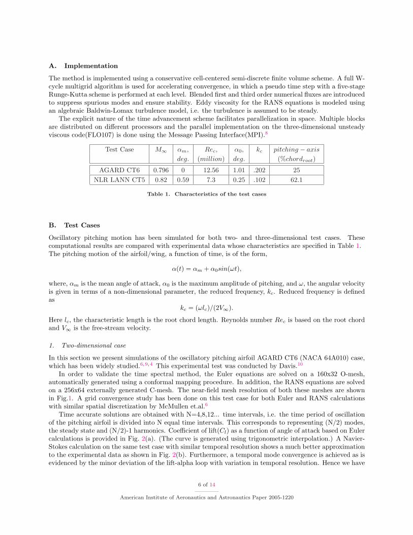
Test Case M∞ αm, Rec, α0, kc pitching − axis

deg. (million) deg. (%chordroot)

AGARD CT6 0.796 0 12.56 1.01 .202 25NLR LANN CT5 0.82 0.59 7.3 0.25 .102 62.1

Table 1. Characteristics of the test cases

B. Test Cases

Oscillatory pitching motion has been simulated for both two- and three-dimensional test cases. Thesecomputational results are compared with experimental data whose characteristics are specified in Table 1.The pitching motion of the airfoil/wing, a function of time, is of the form,

α(t) = αm + α0sin(ωt),

where, αm is the mean angle of attack, α0 is the maximum amplitude of pitching, and ω, the angular velocityis given in terms of a non-dimensional parameter, the reduced frequency, kc. Reduced frequency is definedas

kc = (ωlc)/(2V∞).

Here lc, the characteristic length is the root chord length. Reynolds number Rec is based on the root chordand V∞ is the free-stream velocity.

1. Two-dimensional case

In this section we present simulations of the oscillatory pitching airfoil AGARD CT6 (NACA 64A010) case,which has been widely studied.6,9,4 This experimental test was conducted by Davis.10

In order to validate the time spectral method, the Euler equations are solved on a 160x32 O-mesh,automatically generated using a conformal mapping procedure. In addition, the RANS equations are solvedon a 256x64 externally generated C-mesh. The near-field mesh resolution of both these meshes are shownin Fig.1. A grid convergence study has been done on this test case for both Euler and RANS calculationswith similar spatial discretization by McMullen et.al.6

Time accurate solutions are obtained with N=4,8,12... time intervals, i.e. the time period of oscillationof the pitching airfoil is divided into N equal time intervals. This corresponds to representing (N/2) modes,the steady state and (N/2)-1 harmonics. Coefficient of lift(Cl) as a function of angle of attack based on Eulercalculations is provided in Fig. 2(a). (The curve is generated using trigonometric interpolation.) A Navier-Stokes calculation on the same test case with similar temporal resolution shows a much better approximationto the experimental data as shown in Fig. 2(b). Furthermore, a temporal mode convergence is achieved as isevidenced by the minor deviation of the lift-alpha loop with variation in temporal resolution. Hence we have

6 of 14

American Institute of Aeronautics and Astronautics Paper 2005-1220

NACA 64A010 GRID 160 X 32

NACA CT6 AIRFOIL GRID 256 X 64

Figure 1. Near-field O- and C-mesh resolution

shown that 4 time intervals, or 1 harmonic is sufficient to obtain engineering accuracy for this oscillatorypitching airfoil.

Fig. 3(a) and 3(b) display the coefficient of moment (Cm) data as a function of angle of attack obtainedfrom Euler and RANS calculations. The Cm data differs significantly from the experimental results. Thisis not surprising considering that previous investigators9 using similar spatial discretizations have shownsimilar discrepancies between the experimental data and their time accurate computations.

Fig. 4 and Fig. 5 show the convergence histories of the Euler and RANS calculations for one of the timeinstances. With a 5-level W-cycle multigrid, the Euler calculation converges six orders of magnitude(RMSdensity residual) in 100 multigrid cycles and the RANS calculation converges five orders of magnitude inabout 700 multigrid cycles.

2. Three-Dimensional Case

In this section, we present three-dimensional unsteady results. This test case relates to a semi-span modelof a transport-type wing with a supercritical airfoil section, the LANN wing. Table (1) summarizes thecharacteristics of the central transonic test case CT5 of the experimental program conducted by R.J.Zwaanfrom NLR.11

Unsteady RANS calculations have been performed for flow over the oscillatory pitching LANN wing witha 256x64x48 internally generated C-H viscous mesh, based on a conformal mapping procedure. It should benoted that all computations have been carried out on the theoretical coordinates of the LANN wing, which

7 of 14

American Institute of Aeronautics and Astronautics Paper 2005-1220

−1 −0.8 −0.6 −0.4 −0.2 0 0.2 0.4 0.6 0.8 1

−0.1

−0.05

0

0.05

0.1

Angle of Attack (deg.)

Coe

ffici

ent o

f Lift

4 Time Intervals 8 Time Intervals12 Time Intervals16 Time Intervals24 Time IntervalsAGARD:702−Davis

(a) Euler Calculations

−1 −0.8 −0.6 −0.4 −0.2 0 0.2 0.4 0.6 0.8 1

−0.1

−0.05

0

0.05

0.1

alpha

Cl

4 time intervals8 time intervals12 time intervalsAGARD−702:Davis

(b) Navier-Stokes calculations

Figure 2. Comparison of Cl data with experimental results for the AGARD CT6 test case.

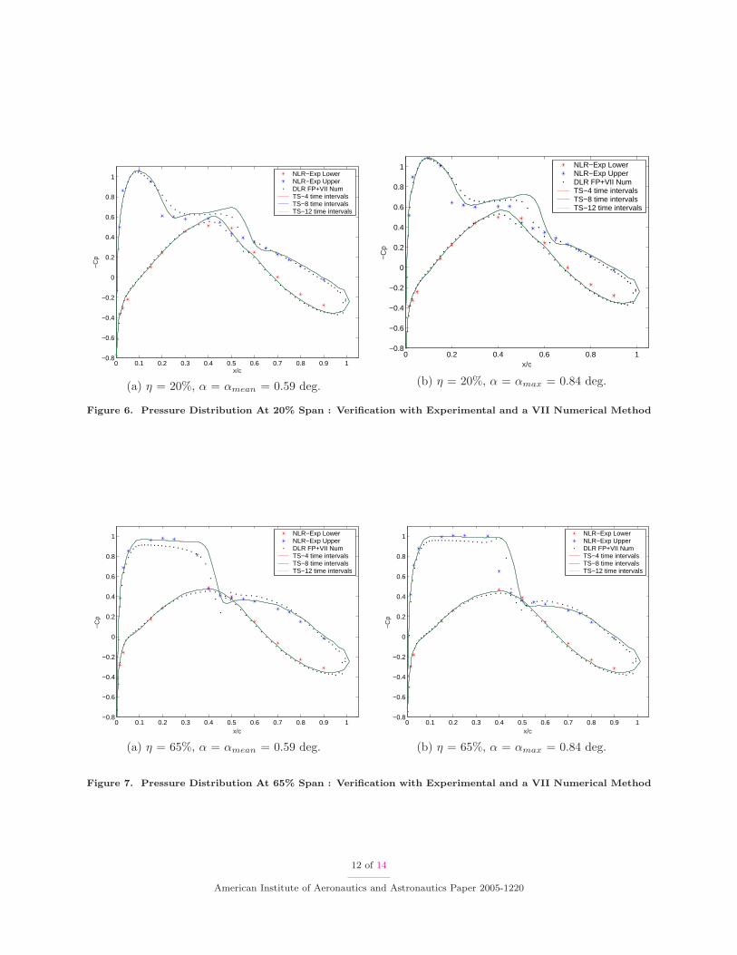
deviate from the measured coordinates. Fig. 6(a) and (b) display the pressure distribution at a 20% spansection at α = αmean and α = αmax respectively. Time spectral solutions with N=4,8 and 12 time intervalsare displayed. Also displayed are the results from another numerical test conducted by DLR WB-AE.12

They use a viscous-inviscid interaction(VII) method, which combines an inviscid(full potential method) anda boundary-layer method by an appropriate coupling approach.

The experiment shows a strong λ-type shock system which has been captured by the numerical results.The pressure peaks have been predicted well, but the location of the shock is not accurate. This couldbe attributed to the algebraic Baldwin-Lomax turbulence model. Note that the time spectral solution hasconverged in temporal resolution. Using 4 time intervals the flow physics has been captured to engineeringaccuracy. Fig. 7 (a) and (b) display a similar pressure distribution at 65% span location.

Fig. 8 shows the convergence history of the RANS calculation on the LANN pitching wing. With a 4-levelW-cycle multigrid, the parallel code converges 5 orders of magnitude in 800 multigrid cycles.

C. Spectral Accuracy

In the previous sections, the time spectral method has been tested and verified with experimental andnumerical results for simple pitching cases which are characterised by an amplitude and a phase. In thesecases it has been shown that 4 time intervals are sufficient to successfully capture the unsteady phenomena.In this section, we will explore a case with a more complicated pitching history, one characterised by manyfrequencies.

We haven chosen a pitching cycle of the form

α(t) =3

5− 4cos(t),

Fig. 9 shows the variation of angle of attack, α, as a function of time for one full period. The timeperiod is 2π. Euler calculations have been performed on the NACA64A010 160x32 O-mesh at free-streamM∞ = 0.796 and pitched about 25% chord.

8 of 14

American Institute of Aeronautics and Astronautics Paper 2005-1220

−1.5 −1 −0.5 0 0.5 1 1.5−0.015

−0.01

−0.005

0

0.005

0.01

0.015

alpha

Cm

4 time intervals8 time intervals12 time intervals16 time intervals24 time intervalsAGARD−702:Davis

(a) Euler Calculations

−1.5 −1 −0.5 0 0.5 1 1.5−0.015

−0.01

−0.005

0

0.005

0.01

0.015

alpha

Cm

4 time intervals8 time intervals12 time intervalsAGARD:702−Davis

(b) Navier-Stokes calculations

Figure 3. Comparison of Cm data with experimental results for the AGARD CT6 test case.

Fig. 10(a) shows the variation of Coefficient of Lift(Cl) as a function of α computed with N=4,8,12,16,20 and24 time intervals per pitching cycle. Note that at least 16 time intervals are required to obtain engineeringaccuracy. 4 time intervals are not sufficient, but increasing N shows an improvement in the solution anda convergence in the right direction. A similar trend is portrayed in Fig. 10(b) which displays the varia-tion of coefficient of moment about the quarter chord, Cm, as a function of α. With higher-order spatialdiscretization, one may obtain spectral convergence in time.

IV. Conclusions and Future Work

The numerical results and their validation confirm the accuracy and computational efficiency of the TimeSpectral Algorithm for unsteady periodic problems. The oscillatory pitching airfoil/wing case showed thatengineering accuracy can be obtained with just four time intervals per period or one harmonic. A goodprediction of the flow around a three-dimensional pitching wing has increased the range of problems thatcan be tackled with this method. Since periodicity is enforced, computational effort towards resolving thedecay of initial transients in minimal. The need for only a small number time intervals to obtain sufficientaccuracy for the globally integrated quantities together with the fact that spectral accuracy can be achievedwith higher order spatial discretization, provides a promising route to more efficient computation of complexperiodic unsteady problems.

The current implementation has an explicit treatment of the time derivative term. This works fine forsmall frequencies and small pitching amplitudes. An implicit treatment of the time derivative is underinvestigation for high frequency applications. A local time-stepping scheme based on the modified stabilityregion, due to the time spectral source term, is also a topic of interest. The current unsteady implementationis very memory intensive, since all the time instances are solved for at the same time and need to be allocatedsimultaneously. Hence, an extension to a large number of time intervals for complex problems might beprohibitive. Nevertheless, this approach can be used with a small number of intervals to provide an initialguess for the standard BDF without having to evolve through transients, and hence provide a much fasterperiodic solution.

Such an efficient method could bring about significant benefits in a wide variety of applications. Theseinclude rotor-stator combinations in turbomachinery, helicopter rotors, aeroelastic problems, flapping wing

9 of 14

American Institute of Aeronautics and Astronautics Paper 2005-1220

NACA 64A010

MACH 0.796 ALPHA 0.000

RESID1 0.368E+01 RESID2 0.627E-06

WORK 99.00 RATE 0.8543

GRID 160X 32

0.00 50.00 100.00 150.00 200.00 250.00 300.00

Work

-.1E

+02

-.1E

+02

-.8E

+01

-.6E

+01

-.4E

+01

-.2E

+01

0.0E

+00

0.2E

+01

0.4E

+01

Log

(Err

or)

-.2E

+00

0.0E

+00

0.2E

+00

0.4E

+00

0.6E

+00

0.8E

+00

0.1E

+01

0.1E

+01

0.1E

+01

Nsu

p

Figure 4. Convergence History - CT6 - Euler

flight, flow control by synthetic jets. The time spectral algorithm has already been implemented successfullyfor low RPM turbomachinery problems. This required a modification of the time spectral algorithm toconform to sector periodicity.13 The algorithm has also been used for research in Vertical-Axis Wind-Turbines14 to study the dynamic motion of a turbine blade spinning about an axis.

V. ACKNOWLEDGMENT

This work has benefited from the generous support of the Department of Energy under contract num-ber LLNL B341491 as part of the Accelerated Strategic Computing Initiative(ASCI) program at StanfordUniversity.

References

1A. Jameson and D.A. Caughey. How many steps are required to solve the euler equations of steady compressible flow:In search of a fast solution algorithm. AIAA paper 01-2673, 15th Computational Fluid Dynamics Conference, Anaheim, CA,June 2001.

2K.C. Hall, J.P. Thomas, and W.S. Clark. Computation of unsteady nonlinear flows in cascades using a harmonic balancetechnique. AIAA Journal, 40(5):879–886, May 2002.

3A. Jameson. Time dependent calculations using multigrid, with applications to unsteady flows past airfoils and wings.(91-1596), June 1998.

4J.M. Hsu and A. Jameson. An implicit-explicit hybrid scheme for calculating complex unsteady flows. AIAA paper 02-0714, AIAA 40th Aerospace Sciences Meeting and Exhibit, Reno, NV, January 2002.

5M. McMullen, A. Jameson, and J.J. Alonso. Acceleration of convergence to a periodic steady state in turbomachinery

10 of 14

American Institute of Aeronautics and Astronautics Paper 2005-1220

0 100 200 300 400 500 600 700 80010

−1

100

101

102

103

104

105

Number of Multigrid Cycles

Log(

Err

or)

Figure 5. Convergence History - CT6 - RANS

flows. AIAA paper 01-0152, AIAA 39th Aerospace Sciences Meeting, Reno, NV, January 2001.6M. McMullen, A. Jameson, and J.J. Alonso. Application of a non-linear frequency domain solver to the euler and

navier-stokes equations. AIAA paper 02-0120, AIAA 40th Aerospace Sciences Meeting and Exhibit, Reno, NV, January 2002.7A.Quarteroni C.Canuto, M.Y.Hussaini and T.A. Zang. Spectral Methods in Fluid Dynamics; Springer Series in Compu-

tational Physics. Springer Verlag, 1988.8Message Passing Interface Forum. MPI: A Message-Passing Interface Standard, March 1994.9N.A.Pierce and J.J. Alonso. Efficient computation of unsteady viscous flow by an implicit preconditioned multigrid

method. AIAA Journal, 36:401–408, 1998.10S.S. Davis. Naca 64a010 (nasa ames model) oscillatory pitching. AGARD Report 702, January 1982.11R.J. Zwaan. Data set 9, LANN Wing. Pitching Oscillation. Technical report, AGARD, 1985. Agard-R-702 Addendum

No.1.12W.Haase, E.Chaput, E.Elsholz, M.A.Leschziner, and U.R.Muller. ECARP: Validation of CFD Codes and Assessment

of Turbulence Models; Notes on Numerical Fluid Mechanics, Vol. 58. Vieweg, 1997.13A. Gopinath, E. Van der Weide, and A. Jameson. Turbomachinery applications with the time spectral method. AIAA

(pending) paper, 17th AIAA Computational Fluid Dynamics Conference, Toronto, Ontario, June 6-9 2005.14J.C.Vassberg, A.Gopinath, and A.Jameson. Revisiting the vertical-axis wind-turbine design using advanced computational

fluid dynamics. AIAA paper 05-1220, 43rd AIAA Aerospace Sciences Meeting and Exhibit, Reno, NV, January 10-13 2005.

11 of 14

American Institute of Aeronautics and Astronautics Paper 2005-1220

0 0.1 0.2 0.3 0.4 0.5 0.6 0.7 0.8 0.9 1−0.8

−0.6

−0.4

−0.2

0

0.2

0.4

0.6

0.8

1

x/c

−C

p

NLR−Exp LowerNLR−Exp UpperDLR FP+VII NumTS−4 time intervalsTS−8 time intervalsTS−12 time intervals

(a) η = 20%, α = αmean = 0.59 deg.

0 0.2 0.4 0.6 0.8 1−0.8

−0.6

−0.4

−0.2

0

0.2

0.4

0.6

0.8

1

x/c

−C

p

NLR−Exp LowerNLR−Exp UpperDLR FP+VII NumTS−4 time intervalsTS−8 time intervalsTS−12 time intervals

(b) η = 20%, α = αmax = 0.84 deg.

Figure 6. Pressure Distribution At 20% Span : Verification with Experimental and a VII Numerical Method

0 0.1 0.2 0.3 0.4 0.5 0.6 0.7 0.8 0.9 1−0.8

−0.6

−0.4

−0.2

0

0.2

0.4

0.6

0.8

1

x/c

−C

p

NLR−Exp LowerNLR−Exp UpperDLR FP+VII NumTS−4 time intervalsTS−8 time intervalsTS−12 time intervals

(a) η = 65%, α = αmean = 0.59 deg.

0 0.1 0.2 0.3 0.4 0.5 0.6 0.7 0.8 0.9 1−0.8

−0.6

−0.4

−0.2

0

0.2

0.4

0.6

0.8

1

x/c

−C

p

NLR−Exp LowerNLR−Exp UpperDLR FP+VII NumTS−4 time intervalsTS−8 time intervalsTS−12 time intervals

(b) η = 65%, α = αmax = 0.84 deg.

Figure 7. Pressure Distribution At 65% Span : Verification with Experimental and a VII Numerical Method

12 of 14

American Institute of Aeronautics and Astronautics Paper 2005-1220

NLR LANN WING UNSTEADY-TIME SPECTRAL

MACH 0.822 ALPHA 0.590

RESID1 0.905E+04 RESID2 0.332E-01

WORK 799.00 RATE 0.9845

GRID 256X64X48

0.00 200.00 400.00 600.00 800.00 1000.00 1200.00

Work

-.1E

+02

-.1E

+02

-.8E

+01

-.6E

+01

-.4E

+01

-.2E

+01

0.0E

+00

0.2E

+01

0.4E

+01

Log

(Err

or)

-.2E

+00

0.0E

+00

0.2E

+00

0.4E

+00

0.6E

+00

0.8E

+00

0.1E

+01

0.1E

+01

0.1E

+01

Nsu

p

Figure 8. Convergence History - LANN - RANS

0 0.2 0.4 0.6 0.8 1 1.2 1.4 1.6 1.8 20

0.5

1

1.5

2

2.5

3

t / pi

Alp

ha

Figure 9. α as a function of time for one period. α = 35−4cos(t)

13 of 14

American Institute of Aeronautics and Astronautics Paper 2005-1220

0 0.5 1 1.5 2 2.5 3

0.1

0.2

0.3

0.4

0.5

0.6

Alpha

Cl

4 time intervals8 time intervals12 time intervals16 time intervals20 time intervals24 time intervals

(a) Cl-α plot

0 0.5 1 1.5 2 2.5 3−0.25

−0.2

−0.15

−0.1

−0.05

0

0.05

0.1

0.15

Alpha

Cm

4 time intervals8 time intervals12 time intervals16 time intervals20 time intervals24 time intervals

(b) Cm-α plot

Figure 10. Validation : Cl-α and Cm-α plots showing spectral convergence

14 of 14

American Institute of Aeronautics and Astronautics Paper 2005-1220