1. Report No. 2. Government Actession No.

TX-95-2911-1

4. Trtle and Subtitle

DEVELOPMENT OF A BONDED CONCRETE OVERLAY COMPUTER-AIDED DESIGN SYSTEM

7. Author(s)

Robert Otto Rasmussen, B. Frank McCullough, and jose Weissmann

9. Performing Organization Name and Address

Center for Transportation Research The University of Texas at Austin 3208 Red River, Suite 200 Austin, Texas 78705-2650

Technical Report Documentation Page

3. Recipient's Catalog No.

5. Report Date january 1995

6. Performing Organization Code

8. Performing Organization Report No.

Research Report 2911-1

10. Work Unit No. (TRAIS)

11. Contract or Grant No.

Research Study 7-2911

t-----------------------------l 13. Type of Report and Period Covered 12. Sponsoring Agency Name and Address

Texas Department of Transportation Research and Technology Transfer Office P. 0. Box 5051 Austin, Texas 78763-5051

15. Supplementary Notes

Interim

14. Sponsoring Agency Code

Study conducted in cooperation with the Texas Department of Transportation. Research study title: "Full-Scale Bonded Concrete Overlay on IH-1 0, El Paso11

16. Abstract

Bonded concrete overlays are increasingly being used to rehabilitate concrete pavements. Among other benefits, bonded concrete overlays (BCO) can reduce life-cycle costs and can expedite construction (thus lowering user costs and delays). Until recently, the design of bonded concrete overlays has been a tedious process. Several design methods are available, including the 1993 Guide for Design of Pavement Structures and the Rigid Pavement Rehabilitation Design System (RPRDS). These design procedures have been automated into a user-friendly software package entitled Bonded Concrete Overlay Computer-Aided Design (BCOCAD). This report documents the development and implementation of the BCOCAD program.

17. KeyWords 18. Distribution Statement

Bonded concrete overlays, rehabilitation strategies, computer-aided design for pavement rehabilitation

No restrictions. This document is available to the public through the National Technical Information Service, Springfield, Virginia 22161.

19. Seturity Classif. {ofthis report)

Unclassified

Form DOT F 1700.7(8-721

20. Security Classif. (of this page)

Unclassified

Reprodudion of <:ompleted page authorized

21. No. of Pages

114

22. Price

DEVELOPMENT OF A BONDED CONCRETE OVERLAY

COMPUTER-AIDED DESIGN SYSTEM

Robert Otto Rasmussen

B. Frank McCullough

Jose Weissmann

Research Report Number 2911-1

Research Project 7-2911

Full-Scale Bonded Concrete Overlay on IH-10 El Paso

conducted for the

Texas Department of Transportation

by the

CENTER FOR TRANSPORTATION RESEARCH

Bureau of Engineering Research

THE UNIVERSITY OF TEXAS AT AUSTIN

January 1995

11

IMPLEMENTATION STATEMENT

The final product of this phase of the project is a comprehensive software package that can be used in the design of bonded concrete overlays (BCO). Because they can reduce life-cycle costs, BCOs have been increasingly used as a method for rehabilitating pavements. The software developed in this project can be used by the Texas Department of Transportation to improve the BCO design for IH-10 in El Paso, and for all similar, future projects.

Prepared in cooperation with the Texas Department of Transportation.

DISCLAIMERS

The contents of this report reflect the views of the authors, who are responsible for the facts and the accuracy of the data presented herein. The contents do not necessarily reflect the official views or policies of the Texas Department of Transportation. This report does not constitute a standard, specification, or regulation.

NOT INTENDED FOR CONSTRUCTION, BIDDING, OR PERMIT PURPOSES

B. F. McCullough, P.E. (Texas No. 19914)

Research Supervisor

iii

iv

TABLE OF CONTENTS

IMPLEMENTATION STATEMENT ............................................................................................ ii SlTMMARY .................................................................................................................................... v

CHAPTER 1. INTRODUCTION .................................................................................................. 1 1.1 Background .......................................................................................................................... 1 1.2 Previous Developments ........................................................................................................ 1 1.3 Objectives ............................................................................................................................. 2 1.4 Scope of Project. ................................................................................................................... 2 1.5 Pavement Rehabilitation Design Methodologies .................................................................. 3

CHAPTER 2. OVERVIEW OF THE BCOCAD SOFTW ARE .................................................. 5 2.1 Software Description and Requirements .............................................................................. 5 2.2 BCOCAD Structure and Installation ................................................................................. ?

CHAPTER 3. MATERIALS IDENTIFICATION AND ANALYSIS ....................................... 13 3.1 Determination of Elastic Moduli ........................................................................................ 13 3.2 Properties of Concrete Pavements ...................................................................................... 16 3.3 Subbase Properties ............................................................................................................. 16 3.4 Subgrade Properties ............................................................................................................ 17 3.5 MATID Module Development. .......................................................................................... 18

CHAPTER 4. TRAFFIC ANALYSIS ......................................................................................... 21 4.1 Analysis Period .................................................................................................................. 21 4.2 Traffic and ESAL Projections ........................................................................................... 21 4.3 TRAFID Module Development ......................................................................................... 22

CHAPTER 5. EXISTING PAVEMENT ANAL YSIS ............................................................... 25 5.1 Pavement Deflection Testing .............................................................................................. 25 5.2 Load Transfer .................................................................................................................... 26 5.3 Remaining Life of the Existing Pavement.. ........................................................................ 27 5.4 Roadway Geometry and Field Surveys .............................................................................. 28 5.5 EXISTID Module Development ....................................................................................... 29

CHAPTER 6. GEOGRAPHIC AND ENVIRONMENTAL INPUTS AND ANALYSIS ....... 35 6.1 Environmental Effects on Pavement Performance ............................................................. 35 6.2 Texas Climatological Database .......................................................................................... 36 6.3 GEOID Module Development ........................................................................................... 37

v

CHAPTER 7. PAVEMENT TEMPERATURE PREDICTION MODEL ............................... .41 7.1 Existing Model .................................................................................................................. 41 7.2 Model Calibration .............................................................................................................. 43 7.3 PA VETEMP Program Development ................................................................................ 43

CHAPTER 8. OVERLAY DESIGN MODULES ...................................................................... 47 8.1 OLDESIGN Program Parameters ..................................................................................... 47 8.2 1993 AASHTO Design Method ....................................................................................... .48 8.3 BCOPRDS Design Method ............................................................................................... 50 8.4 Design Results .................................................................................................................... 51

CHAPTER 9. IMPLEMENTATION ....................................... ., ................................................ 53 9.1 Guidelines ........................................................................................................................... 53 9.2 Pilot Applications .... , .......................................................................................................... 53

CHAPTER 10. CONCLUSIONS AND RECOMMENDATIONS ........................................... 63 10.1 Conclusions ...................................................................................................................... 63 10.2 Recommendations ............................................................................................................ 63

REFERENCES ............................................................................................................................ 65 APPENDIX A: Input File Formats .............................................................................................. 67 APPENDIX B: Sample Output Files ............................................................................................ 73

vi

SUMMARY

Bonded concrete overlays are increasingly being used to rehabilitate concrete pavements. Among other benefits, bonded concrete overlays (BCO) can reduce life-cycle costs and can expedite construction (thus lowering user costs and delays). Until recently, the design of bonded concrete overlays has been a tedious process. Several design methods are available, including the 1993 Guide for Design of Pavement Structures and the Rigid Pavement Rehabilitation Design System (RPRDS). These design procedures have been automated into a user-friendly software package entitled Bonded Concrete Overlay Computer-Aided Design (BCOCAD). This report documents the development and implementation of the BCOCAD program.

vii

viii

CHAPTER 1. INTRODUCTION

1.1 BACKGROUND

Bonded concrete overlays (BCO) have been used for several decades to rehabilitate deteriorating pavement structures. Among other benefits, this rehabilitation technique adds service life to the original pavement structure, thereby reducing the pavement's life-cycle costs. As a result of its increasing use among various state highway agencies and other local government agencies, pavement engineers have developed several BCO design methods. The fact that BCO is considered a viable economical and technical alternative to extending pavement service life has made imperative the development of quick and accurate BCO design options.

The determination of the final thickness to be used on a pavement is often a time­consuming and frustrating effort. In the past, the lack of computerized tools limited the number of alternatives that could be examined by the pavement designer; and the delays to the traveling public, caused by pavement rehabilitation procedures, was, usually, considered irrelevant. Recently, however, user costs have been recognized as an important input to be taken into account in the life-cycle cost analysis of pavement design and rehabilitation alternatives, highlighting the importance of computerized tools that allow the study of several different design alternatives. With the user costs associated with closing a major throughway exceeding tens of millions of dollars per day, minimizing construction delays must be accounted for in the selection of an optimum design.

The combination of a BCO and fast-tracking and construction expediting techniques is an excellent pavement rehabilitation option, especially in urban areas where user-costs are high and the need for a long-lasting pavement rehabilitation technique is fundamental.

One such project is located along a section of IH-10 in the El Paso District. The AADT for this six-lane section, termed the "depressed section," currently exceeds 170,000 vehicles per day for both directions. With the passage of the North American Free Trade Agreement (NAFTA) by the U.S., Canada, and Mexico, trade has increased significantly, along with a corresponding increase in commercial traffic. This is expected to put a further strain on many of the nation's highways. In particular, El Paso and its sister city Ciudad Juarez, because of their location, are expected to handle a greater share of the increased conunercial traffic.

1.2 PREVIOUS DEVELOPMENTS

Several BCO design methods are available today. Acceptance and use of the various methods vary from agency to agency. In Texas, two methods are used. The first is the method outlined in the AASHTO Guide for Design of Pavement Structures (Ref 1 ). The 1993 version of the AASHTO guide includes new guidelines for the calculation of BCO thicknesses. These guidelines, elaborated in a later chapter, use performance statistics from the AASHO Road Test and subsequent pavement monitoring efforts to calculate an appropriate thickness for the BCO based on design inputs.

1

2

Another method used in Texas is one developed by the Center for Transportation Research (CTR) as part of Research Project 249 (Ref 2); it is referred to in this report as the Rigid Pavement Rehabilitation Design System (RPRDS). RPRDS utilizes a more mechanistic approach to predict pavement performance and to design the appropriate cross-section thickness. This method will also be discussed in this report.

With the present widespread use of computers in pavement design, the use of software as a design tool has both increased productivity and optimized pavement design alternatives. Yet the 1993 AASHTO overlay design method has not, to the knowledge of the authors, been incorporated in any software package. RPRDS, however, was computerized in a program called RPRDS-1.

The use ofBCO as the optimum alternative was researched by CTR in Project 1957 (Ref 3). In that study, preliminary overlay thicknesses were developed using pavement deflection data, condition survey results, and pavement core test results. The two methods of pavement design, discussed previously, were used in Project 1957 to determine the optimum thickness of the BCO. It became evident, however, that an improved BCO design tool would improve the productivity and accuracy of the results.

1.3 OBJECTIVES

The purpose of this project was to develop a software tool that could be used not only by engineers working with the BCO project in El Paso, but also by any other Tx.DOT district to quickly and accurately determine BCO thicknesses required for almost any set of design conditions. In addition, the new design tool should provide the user with as much flexibility as possible in designing a BCO. Since the designer is sometimes provided with inadequate information for the design, the software should provide as much guidance as possible in producing an accurate design, given available information.

Future modifications in the software as improvements are made in the design methodology should be relatively easy. The software should be constructed in a manner such that a programmer having moderate expertise can add or revise the existing software.

1.4 SCOPE OF PROJECT

This report documents the development of a bonded concrete overlay computer-aided design system (BCOCAD); it also outlines the philosophy behind the development of BCOCAD; that is, the need to overcome the disadvantages of existing pavement design software by providing the user with a relatively simple, user-friendly, yet powerful tool for the design of BCOs.

BCOCAD includes a full range of user design inputs, allowing as much flexibility as possible in the design of BCOs. In addition, the software was designed so that any future developments, modifications, or additions could be made with relative ease. The details of this software are described in the bulk of this report, using the Interstate highway design in El Paso as an example to demonstrate the capabilities ofBCOCAD.

The following chapters will explain in detail each of the input modules in the BCOCAD software. BCO design, unlike a new construction design, requires additional inputs specific to the

3

existing pavement. These additional inputs, along with the other pavement design parameters, should be entered in a logical fashion in order to minimize error on the part of the designer. Because many existing design programs fail to provide a logical interface, they increase the potential for error.

1.5 PAVEMENT REHABILITATION DESIGN METHODOLOGIES

Several rigid pavement rehabilitation design methods have been developed since the AASHO Road Tests of the 1950s. Many of these design methods are based on data from the Road Test, either directly or indirectly. In addition, attempts have been made to develop a mechanistic design procedure based on a purely theoretical approach. But owing to the number, complexity, and uncertainty of the factors influencing pavement performance, a purely mechanistic model cannot currently be developed. However, some current design methods use a combination of the mechanistic approach and empirical data (to calibrate the model), eliminating some of the differences between the model and the real world.

The AASHO Road Test is the basis for many of the design procedures in use today. This full-scale test was performed from the late 1950s to the early 1960s in Ottawa, lllinois. While the purpose of the test was to quantitatively measure the effect of traffic on both concrete and asphalt pavements, this report will focus on only the rigid pavement design. Test sections of varying dimensions were constructed, with an effort made to ensure uniformity in the quality of the construction materials.

During the test a large volume of data was collected, including distress measurements and quantitative data on the stress conditions of the pavements. The concept of pavement serviceability was introduced at the road test. The serviceability is a measure of the user's satisfaction with the pavement. The results of the Road Test included an attempt to estimate serviceability as a function of the magnitude of the distresses.

AASHTO Design Method

The AASHTO design method was developed directly from the AASHO Road Test data. Regression analyses were performed using the data collected, and design equations were derived. The design equations determined the thicknesses required to sustain a specified level of serviceability over the design life. Although every effort was made to minimize variability in the farge amount of data collected, several deficiencies in this design method exist. These include the fact that the project was subjected to only one set of environmental conditions, including the climate as well as the sub grade type. In addition, only a limited number of material combinations were tried, and therefore other combinations not tested must be interpolated or extrapolated from the results.

The AASHTO method is, thus, empirical in nature. In order for the method to be used, empirical factors must be identified to classify the subgrade, climate, and drainage conditions. In 1986, the concept of reliability was included in the design method. The reliability concept utilized a standard deviation of the materials and traffic measurements, thus adding flexibility to the design. For example, if accurate information about the design inputs cannot be collected, a standard

4

deviation reflecting this inaccuracy can be applied. Conversely, if care was taken to collect this information, the design can be improved by applying a smaller standard deviation, which will result in a thinner cross section.

A reliability factor was also added to provide a statistical measure of the overall design. For example, if prevention of premature pavement failure is critical, a higher reliability can be assigned, resulting in a thicker cross section. This may be true for such facilities as Interstate highways in urban areas. However, if premature failure of the pavement is not a concern (i.e., it is a secondary route), a smaller reliability may be used, resulting in a thinner cross section.

RPRDS Design Method

The RPRDS design system was developed by the Center for Transportation Research to improve TxDOT' s existing pavement rehabilitation procedure. The existing procedure, called the Texas Rigid Pavement Overlay Procedure (RPOD), is a semi-mechanistic pavement design method. The method utilizes elastic layer theory, corrected for such boundary conditions as edges and joints, using regression equations developed through a finite element model. Fatigue relationships developed using the AASHO Road Test data are then used to predict failure. The incorporation of these fatigue relationships implies the empirical nature of this design method. Although the stress and strain predictions are mechanistic in nature, the determination of the failure criteria cannot be directly modeled.

CTR Project 249 improves upon the existing RPOD model by incorporating cost analyses (to determine the optimum design) and by upgrading the mechanistic theory. Currently, three fatigue relationships are built into the RPRDS modeL Two of the three are applicable to bonded concrete overlays: one is for the existing pavement, the other for the overlay. These models predict that a pavement will fail in any area where 50 feet of cracking occurs over 93 m2 (1 000 square feet) of pavement surface. This failure criteria contrasts with that of the AASHTO method, which simply defmes failure as some specified level of serviceability.

CHAPTER 2. OVERVIEW OF THE BCOCAD SOFTWARE

The BCOCAD software described in this report was developed to be used as a tool in the determination of BCO design thicknesses. Initially, the scope of the project was to develop a graphical user interface (GUI) to use as a front end for two well-known and accepted design methods: the 1993 AASHTO Guide for Design of Pavement Structures and the Rigid Pavement Rehabilitation Design System (RPRDS) (Refs 1, 2).

2.1 SOFTWARE DESCRIPTION AND REQUIREMENTS

BCOCAD was developed using Microsoft® Fortran Version 5.1 on an ffiM-PC® compatible 486DX2/50 personal computer with 8mb RAM. Designed for a DOS environment, it can be used on most modern personal computers equipped with the following minimum hardware:

• IBM-PC® Compatible system (386 or better processor recommended)

• Microsoft® compatible mouse (DOS driver loaded)

• VGA monitor and video card with 640 x 480 x 16 color ( 4bit) capability

• One high density 1.44mb (HD) 8.89 em (3 1/2 in.) floppy drive

• At least 2mb hard drive space free

• A "largest executable program size" of at least 300k (see the MEM command in MS­DOS®)

These files are required for BCOCAD execution:

• BCOCAD.EXE

• MATID.EXE

• GEOID.EXE

• TRAFID.EXE

• EXISTID.EXE

• PA VETEMP.EXE

• OLDESIGN.EXE

• AASHT093.EXE

• BCOPRDS.EXE

• BCOPRDS7.EXE

• RESULTS.EXE

• ROMAN.FON

BCOCAD Main Program

Materials Identification Module

Geographic Identification Module

Traffic Identification Module

Existing Pavement Identification Module

Pavement Temperature Prediction Model Program

Overlay Design Module

1993 AASHTO Guide Cross Section Design Program

PRDS (Pavement Rehabilitation Design System) program developed by CTR and modified for BCOCAD

PRDS program using the math coprocessor (80x87) if available

Design Results Module

Microsoft Roman Graphics Font

5

6

• TMSRB.FON

• COURB.FON

• UTSEAL.IMG

• CAR.IMG

• TEXAS.DAT

• PAVMATIN.DAT

Microsoft Times-Roman Graphics Font

Microsoft Courier Graphics Font

4-bit image ofUT Seal

4-bit image of an automobile (Ford Mustang)

Texas climatological database for GEOID

Input file for PA VETEMP.EXE

While not required, these fJ.les are recommended:

• INST ALL.EXE

• GZIP.EXE

• GZIP.DOC

• README.TXT

Installation Program

A Lempel-Ziv coding (J._.Z77) file compression/extraction program

The documentation file for GZIP.EXE

A text file describing the system requirements and installation instructions

These files are not required and need not be included:

• BCOCAD.FOR

• MATID.FOR

• GEOID.FOR

• TRAFID.FOR

• EXISTID.FOR

• PA VETEMP.FOR

• OLDESIGN.FOR

• AASHT093.FOR

• BCOPRDS.FOR

• RESUL TS.FOR

· • INST ALL.FOR

• EXTRLIBS.ZIP

Fortran code for BCOCAD.EXE

Fortran code for MATID.EXE

Fortran code for GEOID.EXE

Fortran code for TRAFID.EXE

Fortran code for EXISTID.EXE

Fortran code for PA VETEMP .EXE

Fortran code for OLDESIGN.EXE

Fortran code for AASHT093 .EXE

Fortran code for BCOPRDS[7].EXE

Fortran code for RESUL TS.EXE

Fortran code for INST ALL.EXE

A PK -Zip® file ( v .2.0+) of the external libraries used in the development ofBCOCAD. Full documentation for the libraries are also included, as requested by the creators of the libraries. Specific libraries used include LIBRY.LIB­LIBRY Fortran Callable Library v5.1 by Dudley J. Benton; ELMOP.LIB ~ ELMOP LIB Microsoft Fortran compatible routines by Michael A. Gerhard; and MOUSE.LIB -Microsoft® Mouse Programmer's Reference Library

These files, which may be created by the BCOCAD software, are not required:

• AASHT093.DAT

• AASHT093.0UT

• BCOINFO.DAT

• MATINFO.DAT

• TRAFINFO.DAT

• GEOJNFO.DAT

• EXISTINF.DAT

• PA VETEMP.OUT

• BCOAM.DAT

• BCOPRDS.DAT

• BCOPRDS.OUT

Input file for AASHT093.EXE

Output file from AASHT093.EXE

Data file from BCOCAD.EXE

Data file from MA TID.EXE

Data file from TRAFID.EXE

Data file from GEOID.EXE

Data file from EXISTID.EXE

Output file from PA VETEMP.EXE

File for BCOPRDS[7].EXE

Input file for BCOPRDS[7].EXE

Output file from BCOPRDS[7].EXE

7

In developing the BCOCAD software, we structured the source code to allow for future modification and additions. In addition, many of the subroutines have a common structure and variables that can be easily traced. The modular structure of the program also greatly improves the ability to perform modifications and additions. Possible additions to future versions of BCOCAD include:

• Extended On-Line Help

• Improved Pavement Temperature Modeling

• Finite Element Modeling of Pavement Stresses

• Early-Age Behavior Modeling

• User Cost Modeling

2.2 BCOCAD STRUCTURE AND INSTALLATION

A graphical user interface (GUI) was used in the development of BCOCAD. The use of a GUI improves the speed and accuracy of the program inputs, with the greatest benefit being user friendliness and acceptability.

Many of the existing design software packages use a command line interface (CLI), which is often difficult to use owing to hardware and software restrictions on cursor movement. The use of the mouse in conjunction with the keyboard, however, improves the communication between the user and the computer.

BCOCAD uses a GUI specially developed for the module-based organization of the software. The basic structure of BCOCAD is shown in Figure 2.1, where the base program, BCOCAD.EXE, calls the main module programs internally.

8

BCOC.ID

:MATID

GEOID

TR.'-\FID

E:\ISTID

PAVETEI\1P

OLDESIGN

AASHT093

BCOPRDS

RESTJLTS

Figure 2.llntemal structure of BCOCAD software

To begin using BCOCAD, users must first install the software on their computer system. An install program has been developed to perform this task automatically (because of the size of the BCOCAD software, most of these flies are compressed). The install program, as shown in Figure 2.2, will copy the required flies to the drive of choice, creating a subdirectory if desired. The install program will then uncompress the necessary flles before returning the user to DOS.

BCOCAD Version 1.8 Install

Install Fran Driue:

Install To Driue:

Install Path Nane:

Use the arrow keys to change values <ESC> Exit <EttTEH> Continue

~COCAD

Figure 2.2 BCOCAD installation program computer screen

II

9

To run the program, the user enters BCOCAD from the DOS prompt. Figure 2.3 is a screen capture of the introduction screen; at this point, pressing any key will continue execution, except for the Escape kill, which will get the user back to DOS.

The main menu ofBCOCAD, shown in Figure 2.4, is in the GUI format. Several features of BCOCAD have been standardized to assist in the execution. Table 2.1 shows the actions by the user, and the reactions of the BCOCAD software to those actions.

Wz!nen by Raben Otto Rosm""sen. E.l.T.

Center for Tran:sportation Researc::h The Universny ofTe""" at Austin

-·=-

Figure 2.3 BCOCAD introduction computer screen

M Materials lclent!fication Mod.ule

GEC•ID !Geographic lclent!ficat!cn Module

I 'TRAF:ID J.Tlraffic lden11fication Mociule

Exi:sting Condltions Identification Mociule

LOAD/SAVE

D~ignData

Pavement Temperature Predlc:itcn Model and Animation (OPTIONAl.)

LDESIGN Pavemern Overlay Oe:sigr> (mu::st Nn all input mociules f'ust)

RESULTS Pavemer.t Oe:sigr> ResultS Mod.ule

Main Menu + Bonded Concrete Overlo;r Computer Aided Oesig!\ Syruo ... - Vernon 1.0 llpll• #I ~-

&:Z::' ....

Figure 2.4 BCOCAD main menu computer screen

10

Table 2.1 Actions by the user and the reactions by the BCOCAD software

Action by User Reaction by BCOCAD Press <Esc> (Escape button) Falls back one level, from sub-module to

module, module to main menu, or to exit the program from the main menu

Mouse click on screen button Performs action described on screen (double-bordered box) button Mouse click on [CONTINUE] screen button Same reaction as pressing <Esc>

(falls back one level) Mouse click on check box a...Jn Selects item next to check box Press Arrow Keys or <Tab> Key within a Field pointer (»»»») is switched between sub-module or a screen requesting field input fields inputs Press <Enter> within a sub-module or a Item marked by a pointer (»»»») is screen requestina field inputs selected for editing Mouse click on [ +] or [-] screen buttons Either increments or decrements the

active field, as designated by the pointer (»»»»)

Mouse click on screen button with Selects button contents as active small red type (text converts to large green type)

The main menu consists of several user buttons to choose from. The [Math Coprocessor Present?] button to the right of the screen will default to the system hardware set up after testing the system's characteristics. If a math-coprocessor is detected internally, it will default to Yes (Y) and if no coprocessor is detected, the button will default to No (N). If for some reason the user would like to change the default setting, clicking the mouse on this button will toggle the setting. However, using the floating point processor or math coprocessor will significantly improve the performance of the design programs. If no coprocessor is present, and the setting is set to Yes, the results may be unpredictable.

The user button just below the co-processor labeled [LOAD/SAVE Design data] allows the user to import or export completed sets of design data. Complete sets must contain all the necessary inputs from all four of the input modules: MATID, GEOID, TRAFID, and EXISTID. This option allows the user to change values in a data set previously entered, without entering all the data from the beginning.

The top four buttons to the left of the screen are the design input modules; Chapters 3 through 6 will elaborate on the specifics of these modules and the sub-modules. If all of the sub­modules within a module have been edited, the module title will become hatched, meaning that the data entry has been completed. In order for the design program to run, all four of the input modules must be hatched, as shown in Figure 2.5.

The [P A VETEMP] button is optional and will run a pavement temperature prediction model and animation program. Additional information on this model is given in Chapter 7. The [OLDESIGN] button performs the design calculations using the design inputs. Further information on this subprogram is included in Chapter 8. The [RESULTS] button will display the results of the BCO design in several formats and is described in Chapter 8 as well.

Materials Identification Module

Geographic Identification Module

Identification Module

Existing Conditions Identification Module

y am::= N

LOAD/SAVE

Design Data

I LDESIGN Pavement Overlay Design (mu:st run all input modules first)

RESUL Pavement Design Results Module

Main Menu ~ Bonded Concrete Overlay Computet Aided Design system- Vernon 1.0 alpha #1 '-.-

..-,=..,""':-

Figure 2.5 BCOCAD main menu computer screen with module buttons hatched

11

12

CHAPTER 3. MATERIALS IDENTIFICATION AND ANALYSIS

Materials characteristics are among the most critical elements of pavement design. Unfortunately, these inputs are often the most difficult to determine accurately. In order to determine the optimum BCO thickness, information must be collected for the subgrade, subbase, existing pavement, and the new overlay pavement. The existing pavement layer materials can be tested in place, or testing records can be used from the original construction. The new pavement materials properties can often be estimated with some precision, based on other construction projects that make use of the same or similar materials.

3.1 DETERMINATION OF ELASTIC MODULI

One of the most convenient ways of characterizing the load-carrying capacity of a pavement stratum is by determining elastic moduli. The modulus of elasticity, a measure of the pavement's stiffness, is defmed as a ratio of the stress to strain. This relationship can be simple (such as characterized by the almost linear stress-strain relationship of steel in the elastic range of loading, where the modulus is simply the slope of the stress-strain line up to the yield point), or more complicated (as is the case for non-linear materials such as concrete).

A typical stress-strain curve for concrete is shown in Figure 3.1. Typical values for the modulus of concrete range from 14 GPa (2000 ksi) to 41 GPa (6000 ksi). Several empirical relationships have been developed to estimate the modulus from other concrete properties. The most common formulae are (Ref 9):

(3.1)

where the modulus, Ec, in psi, is a function of the compressive strength, t' c• in psi, or:

Ec = ( 40, ooo{T: + 1, 000,000 )( l:S) l.S (3.2)

where the modulus is a function of the compressive strength and the unit weight of the hardened concrete, w c• in pcf.

Because the stress-strain relationship for soils is often very complex, a direct definition of the modulus of elasticity is more difficult to ascertain. For a single load application, a soil may react as shown in Figure 3.2. The shape of the curve is highly dependent on many factors, including the density, y, water content, w, and the confining stress level, a3•

The modulus of the soil under a single load application is usually determined from a secant line drawn from the origin to a point on the curve (usually some fraction of the failure stress).

13

14

Figure 3.1 Generalized stress-strain curve for concrete (Ref 9)

Figure 3.2 Typical non-cyclic stress-strain relationship for a soil (Ref 12)

A peculiar property of some soils, however, is the ability to record their load history by changing their internal properties. This is can be illustrated by applying a cyclic load to a typical soil. After each successive load application, the residual strain increases at a decreasing rate. This is shown in Figure 3.3, where the modulus of the soil, determined using the secant method described previously, often increases as the number of loads applied increases.

15

Figure 3.3 Typical cyclic stress-strain relationship for a soil (Ref 12)

The soil modulus, after a given number of load applications, will begin to stabilize in value; this value is usually used to characterize these materials for design purposes.

Most of the pavement design programs use the static (non-cyclic) modulus of elasticity. This value is often easier to determine in laboratory tests, as standardized methods of determining this value have been established.

One of the most common methods of determining the moduli of soils beneath existing pavements is through the use of dynamic deflection data, such as that collected using a falling weight deflectometer (FWD). Chapter 5 explains the specifics of FWD testing.

By using elastic layer theory, moduli can be backcalculated using deflection data and by measuring or estimating other parameters of the pavement layers. RPEDDl and MODULUS are two computer programs that will perform the backcalculation procedure using FWD data. Since the backcalculation of moduli values from deflection data is numerically intensive, computer programs often save a significant amount of time in the data analysis process (Refs 10, 11 ).

Another method of determining moduli values is through materials testing. The modulus of paving concrete can be determined be testing cores taken from the existing pavement; the concrete to be used in the overlay can be tested by casting standard cylinders.

Subbase and subgrade moduli and other properties can also be determined from collection of samples from the field, though this option is often expensive and unnecessary if deflection data can be collected.

16

3.2 PROPERTIES OF CONCRETE PAVEMENTS

Besides the modulus of elasticity of the concrete, several other materials properties should be known prior to the pavement design. These include Poisson's ratio and the flexural strength of the concrete.

The concrete Poisson's ratio, though not a critical input in pavement design, is used in determining moduli values through deflection data backcalculation procedures. The Poisson's ratio value is often estimated to be 0.15 to 0.20, but can actually vary between 0.15 to 0.25; it is a function of the aggregate used, moisture content, concrete age, and compressive strength (Ref 9).

The flexural strength of concrete, or modulus of rupture, is often used to classify the quality of the paving concrete. In order to determine the flexural strength directly, beams are either cut from the existing pavement, or cast using the overlay concrete. If the flexural strength is not determined directly, it may be estimated from another concrete property, such as the compressive strength; this relationship, for normal-weight concrete, is (Ref 9):

(3.3)

where the modulus of rupture, S · c• is a function of the compressive strength, r' c·

Another method of calculating the flexural strength uses the modulus of elasticity, Ec, as shown in Equation 3.4 (Ref 9).

(3.4)

Typical values for the flexural strength of concrete range from 3.5 MPa (500 psi) to 8.3 MPa (1200 psi).

CTR Research Project 1244 has produced some alternative methods for determining the material properties of concrete. For example, a computer program was developed that can predict the concrete properties as a function of the coarse aggregate type used. The program, CHEM, uses oxide residue values from a mineralogical analysis of the aggregate. These values are used in a complex regression analysis that results in strength, modulus, and shrinkage values for the concrete mix using the particular aggregate (Ref 19).

3.3 SUBBASE PROPERTIES

Subbase materials can vary widely from project to project. In some cases, a subbase may not even exist. The subbase may range in quality from a medium-to-low-grade select material up to a high strength cement or asphalt-treated base. The design inputs for subbase include the modulus of elasticity and Poisson's ratio. Table 3.1 shows some common subbase materials and typical elastic modulus values and Poisson's ratios.

Table 3.1 Typical modulus of elasticity of various subbase materials (Ref 1)

Subbase Trpe Cement Treated

Bituminous Treated

Lime Treated

Granular

Fine Grained I Natura1 Subgrade

3.4 SUBGRADE PROPERTIES

Poisson's Ratio 0.20 to 0.30

0.25 to 0.35

0.35 to 0.45

0.30 to 0.50

0.40 to 0.50

Modulus of Elasticity 6.9 GPa (1,000 ksi) to 13.8 GPa (2,000 ksi) 2.4 GPa (350 ksi) to 6.9 GPa (1,000 ksi) 140 :MPa (20 ksi) to 480 MPa (70 ksi)

100 :MPa (15 ksi) to 310 :MPa (45 ksi) 21 :MPa (3 ksi) to 280 :MPa (40 ksi)

17

The subgrade reaction to loading can be classified using two different quantities. The first is the modulus of elasticity, or more commonly known as the Resilient Modulus when referring to subgrades. The second is a modulus of subgrade reaction.

The resilient modulus can be determined in the laboratory using a triaxial device and by applying a repeated axial deviator stress and measuring the recoverable axial strain (Ref 13). The resilient modulus, MR, is then calculated as:

(3.5)

where crd is the deviator stress and £a is the recoverable axial strain. The second value that can be used to classify the quality of the subgrade is the modulus of

subgrade reaction. This concept is shown in Figure 3.4.

Figure 3.4 Modulus of subgrade reaction, ks

18

The modulus of subgrade reaction can vary widely, but is often in the range of 27 MN/m3

(100 pci) to 270 MN/m3 (1000 pci). An empirical conversion from resilient modulus, MR, in psi, to modulus of subgrade reaction, k, in pci, is shown in Equation 3.6 (Ref 1).

k= MR 19.4

(3.6)

The Poisson's ratio for the subgrade can also vary widely depending on many factors, including the quality of the subgrade. Typical values range from 0.3 for high quality sub grades to 0.5 for poor quality.

3.5 MATID MODULE DEVELOPMENT

MATID (MATerial IDentification) is the BCOCAD Module that determines the characteristics of the pavement materials, both existing and for the overlay to be placed. This module is divided into five sub-modules:

• General Materials Information

• Overlay Materials Information

• Existing Pavement Materials Information

• Subbase Materials Information

• Subgrade Materials Information

An example of the MATID main menu is shown in Figure 3.5. The sub-modules are enclosed in user button boxes, which, after being completed, become hatched. As with the other modules, all sub-modules must be completed in order for the data entry to be completed.

The General Materials Information sub-module prompts for information not covered by the specific materials identification sub-modules. The computer screen for this sub-module is shown in Figure 3.6, where the overall standard deviation is the standard deviation defined in the AASHTO design procedure. The magnitude of this value quantifies the deviation from the norm in the material properties. Appendix EE of the 1986 AASHTO Guide describes in detail the procedure to accurately determine this value (Ref 14). If a detailed investigation is not warranted, Table 3.2 can be used to select an appropriate value for the standard deviation for rigid pavements (Ref 14).

Table 3.2 Standard deviation values for various conditions

Condition Range of values If variance of projected future traffic is being considered If variance of projected future traffic is not considered

Standard Deviation, So 0.30 to 0.40

0.39 0.34

19

The loss of support factor is an index factor to detennine the quality of the base support to the existing pavement (this factor is also included in the AASHTO design method). This factor can be detennined directly by using FWD readings taken at joint corners for JRCP and JCP pavements. If loss of support is detected, measures should be taken to eliminate it before the construction of the overlay. It is therefore recommended that a loss of support value of zero (0) be used for the overlay thickness design, unless desired otherwise.

The coefficient of drainage, also an AASHTO design parameter, describes the quality of the subdrainage for the existing pavement. During the condition survey of the existing pavement, drainage conditions should be carefully observed; if any localized problems exist, measures should be taken to eliminate or reduce their adverse effects on the pavement structure before construction of the overlay. Tell-tale signs, such as base pumping or localized cracking, often signify a possible drainage problem. If only a preliminary pavement design is being performed, or if no further information is available to the pavement engineer, Table 3.3 can be used in the selection of an appropriate value for the coefficient of drainage.

Table 3.3 Recommended values of drainage coefficient, Ccf,for rigid pavement design (Ref 1)

Quality of Drainage Excellent

Good Fair Poor

Very Poor

Percent of Time Pavement Structure is Exposed to Moisture Levels Approaching Saturation

Less Than 1%

1.25-1.20 1.20-1.15 1.15-1.10 1.10-1.00 1.00-0.90

1-5% 5-25%

1.20-1.15 1.15-1.10 1.10-1.00 1.00-0.90 0.90-0.80

1.15-1.10 1.10-1.00 1.00-0.90 0.90-0.80 0.80-0.70

Greater Than 25% 1.10 1.00 0.90 0.80 0.70

The computer screen for the second sub-module, Overlay Materials Information, is shown in Figure 3.7. The modulus of elasticity for the concrete to be used in the overlay can be entered either directly or by using an empirical relationship with either the flexural strength, compressive strength, or indirect tensile strength of the concrete. This value, as discussed in Section 3.1 and 3.2, is critical; care should thus be taken in its determination.

The Poisson's ratio is also entered here for the overlay concrete. The flexural strength can also be entered directly or estimated using the modulus of elasticity, compressive strength, or indirect tensile strength of the concrete. If either the modulus or the flexural strength is estimated using the compressive strength or the indirect tensile strength, the appropriate fields appear to the user for input. Equations 3.1, 3.3, 3.4, and 3.7 are used by the program to derive the empirical relationships between these various concrete parameters.

s·c = 210+ 1.02/T (3.7)

20

The flexural strength, S · c• in psi,. is a function of the indirect tensile strength, IT, in psi. The Existing Pavement Materials Identification sub-module, whose computer screen is

shown in Figure 3.8, includes the same inputs as the overlay materials identification sub-module, with two additional fields: the critical stress factor and the concrete stiffness after cracking.

The critical stress factor in the PRDS design model is used by the fatigue model to estimate the stress condition. This factor is defined as the ratio of the critical stress to the interior stress in the existing pavement. Table 3.4 contains recommended values for this parameter (Ref 2).

Table 3.4 Existing pavement critical stress factors (Ref 2)

Existing Pavement Type Existing PCC Range of Critical Shoulders Stress Factor

CRCP No 1.20- 1.25

Yes 1.05- 1.10

JCP No 1.25- 1.30

(with load transfer) Yes 1.10- 1.20

JCP No 1.50- 1.60

(without load transfer) Yes 1.40- 1.50

The concrete stiffness after cracking is a parameter that describes the condition of the pavement after loss of load-carrying capacity. For CRCP, a value of 5.5 GPa (800,000 psi) is recommended; for JCP, a value in the range of 2.1 GPa (300,000 psi) to 3.4 GPa (500,000 psi) is recommended. Unless the edge-to-interior-deflection ratio is high (greater than 1.5), or if major distress repairs are not completed prior to overlay, a higher value should be used (Ref 2).

Figure 3.9 depicts the computer screen for the Subbase Materials Identification sub­module. The two parameters required are the elastic modulus and the Poisson's ratio, which were explained in more detail in Sections 3.1 and 3.3.

The Subgrade Materials Identification sub-module computer screen is shown in Figure 3.1 0. The user button in the middle of the screen detennines the sub grade load reaction parameter to use. The resilient modulus, described in Sections 3.1 and 3.4, may be used; a corresponding k­value will be calculated, internally factoring in the subbase depth and modulus and the depth to bedrock, if applicable. If the modulus of subgrade reaction, k, is chosen as the subgrade parameter, it should be noted that the k value entered should be for the subgrade material only, and not an equivalent k factor for the slab support. Influences on the k factor from subbase and bedrock depth should be neglected. The Poisson's ratio for the subgrade is also entered, as discussed in Section 3.4.

CHAPTER 4. TRAFFIC ANALYSIS

4.1 ANALYSIS PERIOD

Rehabilitation projects require many of the same decisions required in new construction projects. One of the most important decisions associated with both is the establishment of a design life for the pavement. In recent years, more emphasis has been placed on the use of an analysis period that encompasses the design life of the original pavement, combined with one or more rehabilitation or reconstruction periods.

In the past, pavements for even moderate-to-heavy-use facilities were often designed for no more than 20 to 25 years of service - a short life by today' s standards. Over the past two decades, however, pavement engineers have increasingly incorporated user costs into a pavement's life-cycle cost analysis. Since construction on major urban thoroughfares can drive user costs to beyond $10 million per day, the economic implications of such delays called for longer design lives.

One way of minimizing the full system costs (agency and user costs) over an analysis period is to construct or reconstruct pavements using high quality materials; because such pavements require less maintenance, they minimize reconstruction delays and associated user costs. In many cases, however, the analysis period is set to be equal to the design life of a particular alternative. Therefore, other alternatives having shorter lives may be compared by factoring them into the longer analysis period. For example, a BCO having a design life of 30 years may be compared with a series of three ACP overlays, each with a design life of 10 years. The costs can then be compared using either net present values, or equivalent uniform annual costs; these methods are explained in more detail in the AASHTO Guide (Ref 1).

4.2 TRAFFIC AND ESAL PROJECTIONS

One of the most critical, yet difficult to determine, aspects of any pavement design is the estimation of future traffic and the associated loadings, which are often measured in equivalent 80-kN (18-k.ip) single axle loads (ESALs). Usually, in this procedure, traffic counts, expressed in annual average daily traffic (AADT), are determined in order to estimate the user delay and associated costs imposed by construction.

Pavement design is highly dependent on the number of ESALs that the pavement will experience during the analysis period. The calculation of this cumulative value involves two unknowns: the current level of traffic loadings and the growth rate of the loadings.

The current magnitude of the traffic loadings can be determined through several methods. The first one, which makes use of pure engineering common sense, considers the type of facility, location of the facility, and percentage of trucks, among other factors. This method is not acceptable for final analysis, unless low volume and/or light-duty use is expected on the facility.

Greater accuracy can be achieved through a quantitative study of the traffic. This type of study often requires vehicle counts (sub-divided into vehicle classification) over a short period. By

21

22

assuming the number of ESALs per vehicle in each category, one can determine traffic loadings. This method, though more accurate than the previous one, is nonetheless flawed in some respects. For example, the short duration of the traffic study can often lead to a biased result in the traffic flow results (i.e., the level of reliability is a function of the length of the study). In addition, assumptions need to be made as to the average traffic loading per vehicle in each category. This method of analysis is acceptable for all but the heavy-duty facilities.

The most accurate (and most expensive) method of determining traffic loadings is through the use of a weigh-in-motion (WIM) device. Many types of W1M devices are available with variable quality and accuracy (Ref 15). WIM data can provide a very accurate estimate of traffic loadings on the facility.

The current level of traffic loadings, however, is only one input in the forecasting of traffic loadings for pavement design. The second input required is an estimate of the growth rate for the traffic loadings. The models for forecasting growth of both traffic volumes and traffic loadings can assume many mathematical forms. The growth functions for traffic counts are usually easier to determine than those for traffic loadings, owing to the availability of past traffic counts from planning studies.

To determine the growth in traffic loadings, a relationship should be determined between the traffic counts and the traffic loadings (Ref 1 ). The traffic growth function can take many forms: For example, sometimes a linear trend is evident from the analysis of historical traffic data.

The second and most common model for traffic growth is an exponential model. Mathematically, this model assumes that the logarithm of the traffic is proportional to the time. This type of model is often used for areas that are experiencing moderate to rapid development.

Another model of traffic growth occurs when development of an area is light or possibly declining. This type of model demonstrates a slow decline in growth, and can be expressed mathematically as a quadratic function.

The combination of early rapid development, followed by a slow reduction in development, then followed by an equilibrium or steady-state condition, can be defined mathematically by a logistic model. This model is characterized by its distinctive S-shape.

The selection of the appropriate model to explain traffic growths is crucial. It should be noted again that, since the growth model is often defmed for traffic counts, care should be taken in relating this to a growth in traffic loadings. The steady increase in traffic loadings on national highways, together with the increased trade resulting from the North American Free Trade Agreement, will lead to a greater average load per vehicle; thus a higher growth rate for traffic loadings could be warranted.

4.3 TRAFID MODULE DEVELOPMENT

TRAFID (TRAFfic IDentification) is the BCOCAD module that defines the traffic characteristics and the analysis periods (or time constraints) for the pavement design. This module, shown in Figure 4.1, is divided into two sub-modules: time constraints and traffic

23

variables. The first sub-module, time constraints (see Figure 4.2), requests two values. The frrst is the analysis period, in years, which is explained in detail in Section 4.1. AASHTO has established guidelines for selecting the analysis period for the design of pavement structures, as shown in Table 4.1.

Table 4.1 Typical analysis periodsforvariousfacility types (Ref 1)

Highway Conditions

High-volume urban

High-volume rural

Low-volume

Analysis Period ( vears)

30-50

20-50

15-25

The second input in this sub-module is the maximum number of years of heavy maintenance after loss of structural load-carrying capacity. This input is used by the BCOPRDS program in determining the optimum overlay and overall maintenance costs. By increasing this factor, distresses- and therefore costs- will increase (Ref 2); the default value of 4 years may be used if no further information is available.

The second sub-module, traffic variables, contains six user fields and five user buttons. This sub-module, shown in Figure 4.3, prompts for all of the applicable traffic variables used in the pavement design; these include both traffic counts as well as traffic loadings.

The first field is for the Present AADT. This value must be for both directions, all lanes. Oftentimes this is the value provided to the user by the planning agency. The growth rate of the AADT is the second field, for which BCOCAD assumes an exponential growth model. While the AADT is not currently used by the design model, it is expected to be used in future versions of BCOCAD for the calculation of user delays and associated costs.

The next two user inputs are for traffic loadings. To provide the user with as much flexibility as possible in defining this parameter, five user buttons encompassing two categories have been provided. The frrst category allows the user to supply either a traffic loading value (in equivalent 80-k:N [18-kip] single axle loads, or ESALs) as a single year value or as a cumulative value. For the single-year option, the user may select the year the single ESAL value shall represent. For example, if it is determined that in the year 2000, the ESALs will be 15 million per year, and the project is to be constructed in 1995, a value of 15 million can be entered in the 80-k:N ( 18-kip) ESALs field. The top check box can then be marked, and then incremented to year 5 using the [ +] and [-] buttons. Year 5 would represent the difference between 1995 and the year 2000. This feature of the program can be observed in Figure 4.3.

A cumulative value for the ESALs may also be entered. This cumulative value must be over the analysis period defmed in the Time Constraints sub-module.

24

The second category of user buttons presented in Figure 4.3 defines which lane configuration the traffic loading represents. The first check box allows a value to be entered that encompasses all lanes in both directions. The second check box is for traffic in all lanes in a single direction; the final check box is for traffic in the design lane only.

The growth rate incorporated in the model for the 80-k:N (18-kip) ESALs is also assuming an exponential growth model. The user is, however, provided with an option for entering the cumulative value of ESALs over the analysis period. In doing this, an exponential growth curve is fit so that the sum of the ESALs over the analysis period is equal to the value entered. The BCOPRDS uses an exponential growth model internally to calculate the overlay thickness; therefore, an exponential growth curve must be fit to the conditions specified. By observing the charts provided by the computer screen of the traffic variables sub-module, a reasonable growth rate can be estimated that satisfies the cumulative ESALs and that produces reasonable yearly values.

The fifth user input for the traffic variables sub-module is the directional distribution. This input is often set at 50 percent, since the traffic over the long term is essentially equal in both directions. This may be higher, however, if unusual conditions warrant. For example, if the proposed project is near a major industrial facility, the traffic loadings may be higher for one of the directions. This is often the case for roads serving ports, shipyards, or major industrial facilities where trucks arrive loaded and leave the facility unloaded.

Lane distribution is the final input for this sub-module. This input is dependent on many factors, including the number of lanes on the facility and the use of the lanes by trucks. For example, in urban areas, the through trucks will often use the inside lanes of a road facility to avoid traffic weaving at ramps, providing a more even distribution of traffic loads and thus a lower lane distribution factor. In rural areas, however, the reverse is often true, with the lane distribution factor accordingly higher. AASHTO recommends lane distribution factors based on the number of lanes on the facility. These factors, presented in Table 4.2 , should be used with caution, since they are also dependent, as discussed previously, on other factors.

Table 4.2 Typical lane distribution factors determined by number of lanes in each direction

(Ref 1)

Number of Lanes in Each Direction

1

2

3

4

Percent of 80-kN (18-kip) ESAL in Design Lane

100

80-100

60-80

50-75

CHAPTER 5. EXISTING PAVEMENT ANALYSIS

The condition and geometry of the existing pavement are crucial factors in the determination of an appropriate overlay thickness. Most design procedures, including both the 1993 AASHTO procedure and the PRDS procedure, require these inputs to some degree.

Two methods of data collection are often used in combination to obtain the necessary inputs for the pavement design. The first, pavement deflection testing, is a quantitative measure of the response of the pavement system to a dynamic load. Measuring the deflections at fixed intervals from an applied dynamic load, and valuable information can be extracted from this type of test. The second type of data collection procedure often used is a visual condition survey. Although this type of analysis is more qualitative in nature, the results benefit the pavement design procedure significantly and therefore provide a better design.

5.1 PAVEMENT DEFLECTION TESTING

Deflection tests are often among the first performed on a pavement rehabilitation candidate. While network deflection testing is performed on many highways statewide for pavement management purposes, the data obtained are usually inadequate for overlay design. In order to accurately assess the condition of the existing pavement, deflection testing should be performed in shorter intervals within the proposed project boundaries.

Depending on the length of the project, pavement type, project importance, and available monies, the deflection testing interval could range from every 10 meters (30 feet) to every 150 meters (500 feet). Measurements should be taken along continuous spans of pavement (with no intermediate cracks between the deflection sensors) to accurately determine elastic layer moduli. Measurements are also taken across cracks, with the results used to calculate the load transfer at the cracks or joints.

Currently, two different devices are available for measuring dynamic deflections. The first, the Dynaflect, is a light-load (225 N [1000 lb]) vibratory deflection device that is not recommended (owing to its load constraints) but nonetheless often used for testing concrete pavements. On concrete pavements, a load of 4 kN ( 18,000 lb) is recommended to ensure the accuracy of the backcalculated elastic moduli (Ref 4). The falling weight deflectometer (FWD) is usually the device of choice (TxDOT currently has several FWDs in inventory). Figure 5.1 shows a schematic of a Dynatest FWD. With this device, the load is applied once by dropping a fixed weight from a given vertical distance from the pavement. The pavement response is measured as deflections by geophones at fixed distances from the load along the pavement.

25

26

Figure 5.1 Schematic diagram ofDynatest Model8000 FWD (Ref5)

5.2 LOAD TRANSFER

Among other important data, pavement deflections can reveal average load transfer efficiency for the pavement joints and/or cracks. Load transfer is often measured as load transfer efficiency (L TE), which is defined as the percent deflection that is measured on the loaded side of the crack or joint versus the unloaded side; this relationship is calculated by Equation 5.1

(5.1)

where d.Lm and dUm are the deflections measured on the loaded and unloaded slab at the joint or crack, and d.Lj and dUj are the corresponding deflections at a mid-span (non-cracked). The use of the FWD in determining load transfer efficiency is illustrated in Figure 5.2.

Figure 5.2 FWD load plate and deflection sensor locations for joint load transfer efficiency evaluation (Ref 5)

27

Instead of a load transfer efficiency, AASHTO utilizes a J-factor that is an empirical factor. Table 5.1 outlines the recommendations in the 1993 AASHTO Guide to convert from percent load transfer to a load transfer coefficient, also known as a J-factor (Ref 1).

Table 5.1 Conversion from pavement type and percent load transfer to J-factor

Pavement Type CRCP

JPCP (CPCD) or JRCP

Percent Load Transfer NIA > 70

50-70 <50

J·Factor 2.2 to 2.6

3.2 3.5 4.0

A research project undertaken by CTR developed equations to predict the AASHTO load transfer coefficient (J-value) based on field measurements made on rigid pavements using the FWD (Ref20).

5.3 REMAINING LIFE OF THE EXISTING PAVEMENT

Remaining life is one of the most important factors considered in the development of the overlay thickness design. The general AASHTO equation for overlay thickness is shown in equation 5.2

(5.2)

where the overlay thickness, D0~o is equal to the thickness required for the pavement if it were constructed new, De. minus a condition factor, CF, multiplied times the existing pavement thickness, D. The condition factor is directly related to the remaining life of the pavement, as shown in Figure 5.3. From the AASHTO equation, it is evident that an accurate determination of the remaining life is crucial for the development of the overlay design.

iL g

0.9

0 0.8 0 {t

"' 0 = 0.7 '0

8 0.6

0.5

-r--1--1--' ..............

""' ...........

" 1\ \

100 90 80 70 60 so 40 30 20 10 0

% Remaining Ufe (%RL:

Figure 5.3 Relationship between condition factor and remaining life (Ref 1)

28

Remaining life can be determined using many different methods. The least precise method uses a visual condition survey in combination with empirical equations to determine distress indices. The results of the condition survey, combined with the age of the pavement and the cumulative traffic estimates, can be used to predict remaining life factors (Ref 7). Because this type of analysis relies on both partially qualitative measurements and empirical equations, it is often not very reliable.

Another commonly used method utilizes a mechanistic fatigue model, where the general equation for the remaining life model is (Ref 8):

( n18 '\

RL= 1--jx100 N18

(5.3)

In this equation, n18 is the accumulated past traffic in 80-kN (18-kip) ESAL, and N18 is the design fatigue life of the existing pavement in 80-kN ( 18-kip) ESAL.

While the remaining life calculated from this model is more realistic, it still may not be valid, because of the assumption that N18 is the number of ESALs required to carry the pavement to failure, where pavement failure is defmed by the minimum acceptable Pavement Serviceability Index (PSI).

CTR has recently developed a model to predict remaining life of a pavement based on existing databases for rigid pavements in Texas. The current model can predict the remaining life of continuously reinforced concrete (CRC) pavements based on condition survey data of transverse crack spacings (Ref 22). Transverse crack spacings have been found to be the critical factor in determining the failure rate of a CRC pavement (Ref 21). Therefore, it can be directly related to the expected future performance of the pavement and thus, the remaining life.

While other methods exist, they are outside the scope of this study (Ref 1). It is important, however, that care be taken in determining these values, since the fmal overlay design thickness is dependent on these values.

5.4 ROADWAY GEOMETRY AND FIELD SURVEYS

The geometry of the proposed project must also be determined as accurately as possible. The length of the project should be surveyed, and cores should be taken at various intervals to determine the in-situ layer thicknesses. Often, the as-built plans for the project are inaccurate, requiring that additional measures be taken to ensure reliable design parameters. In addition to determining layer thicknesses, cores can also be used in the laboratory to determine the materials properties of the existing layers, as discussed in Chapter 3.

During the field survey of the proposed project, the surrounding area should be noted. Drainage conditions, heaving, pumping, lane-lane or lane-shoulder drop-off, median and shoulder conditions - all should be noted, since they may influence overlay thickness decisions.

29

5.5 EXISTID MODULE DEVELOP:MENT

EXISTID (EXISTing pavement IDentification) is the BCOCAD module that detennines the condition of the existing pavement. This module is subdivided into four sub-modules that defme the following:

• Project Description

• Roadway Geometry

• Roadway Condition

• Roadway Cross Section

The computer screen for the EXISTID main menu is shown in Figure 5.4.

; ¥ #

Roadv:ay Geometrj.' ' .. ' ,~ ' ~ ' ' .- ' '

Figure 5.4 EXISTID main menu computer screen

30

Figure 5.5 Project description sub-module computer screen

The Project Description sub-module, as shown in Figure 5.5, prompts the user for a three­line project description. Within this range, information such as the project title or identification number, dates, or names of personnel involved may be entered. This input will not affect the fmal design; it will serve only as a way to refer to the design. The Project Location may include the highway number, station numbers, centerline offsets, and direction, if appropriate; this field also does not affect the outcome.

Roadway Geometry is input in the second sub-module, as shown in Figure 5.6. The number of lanes in a single direction, project length, lane width, and shoulder width are input in this sub-module. The shoulder width required is for the inside shoulder only. As the modifications are made to the shoulder and lane widths (including number of lanes), the picture of the roadway on the computer screen changes dynamically. All of the plan dimensions are shown on the picture.

Figure 5.7 shows the Roadway Condition sub-module. The number of existing defects per mile is the main variable handled by this sub-module. The defects to be considered are those that will require repair prior to the placement of the BCO. These defects include, but are not limited to, punchouts, severe spalling, blow-ups, and severe localized cracking. The average cost of repairing a defect is also entered, but is not used in determining the overlay thickness (though it can be used to perform a life-cycle cost analysis of the alternatives). The user is also prompted for the rate of defect development; again, the plot of defects per mile changes on the screen dynamically as the

31

inputs are changed. The 1 0-year projection allows the user to envision the magnitude of the number of defects at some future date.

Figure 5.6 Roadway geometry sub-module computer screen

Figure 5. 7 Roadway condition sub-module computer screen

32

The final prompts for the Roadway Condition sub-module, shown in Figure 5.7, are used to calculate the effective depth of the existing pavement. As determined by the status of the user button at the middle of the screen, either a percent remaining life or the 1993 AASHfO adjustment factors may be entered (the remaining life concept was briefly discussed in Section 5.3). The adjustment factors can be determined using the 1993 AASHfO Guide as a reference. The three adjustment factors are defmed in the AASHfO Guide as follows (Ref 1 ):

• Fjc - Joints and cracks adjustment factor- adjusts for the extra loss in PSI caused by deteriorated reflection cracks in the overlay that will result from any unrepaired deteriorated joints, cracks, or other discontinuities in the existing slab prior to overlay.

• Fdur- Durability adjustment factor- adjusts for the extra loss in PSI of the overlay when the existing slab has such durability problems as "D" cracking or reactive aggregate distress.

• Frat - Fatigue damage adjustment factor- adjusts for past fatigue damage that may exist in the slab (e.g., cracking).

Each factor ranges from 0 to 1, its actual value depending on specific criteria outlined in the AASHfO Guide. Since the AASHTO design method uses the adjustment factors and the PRDS methodology uses the remaining life concept, the corresponding values are calculated internally by BCOCAD.

The final sub-module, whose computer screen is shown in Figure 5.8, describes the Roadway Cross Section. The four user buttons at the mid-screen are:

• Pavement Type: CRCP, JRCP, or CPCD (JPCP/JCP)

• Shoulder Type: ACP or PCCP

• Load Transfer from the Lane to the Shoulder: Yes or No

• Load Transfer Variable to use: J-Factor or Percent Load Transfer

The Load Transfer Variable button determines the first input to this sub-module. Either a J-Factor or a Percent Load Transfer may be entered. The value not entered will be calculated internally, since the different design methods use the different input types. The layer thicknesses are also input in this screen, with both the existing pavement and subbase thicknesses input in inches, while the subgrade thickness, if applicable, is input in feet. The subgrade may be assumed to be semi-infinite by entering 99 feet, which will appear as an infinity symbol both on the input line as well as in the diagram. The diagram to the right of the mid-screen will dynamically change as the inputs are changed; this screen prevents erroneous inputs by providing the user with a visual representation of the existing pavement.

33

Figure 5.8 Roadway cross-section sub-module computer screen

34

CHAPTER 6. GEOGRAPHIC AND ENVIRONMENTAL INPUTS AND ANALYSIS

BCOCAD was designed to facilitate future additions and improvements. The geographic and environmental input module, GEOID, was developed to serve as a platform for proposed additions to BCOCAD. Currently, GEOID does not affect pavement design results. It does, however, serve to provide inputs for the pavement temperature prediction model, PA VETEMP, which is explained in Chapter 7. We propose that future versions of BCOCAD include a construction guidelines module capable of modelling ideal environmental conditions for BCO construction; such a module would minimize thermal and/or shrinkage associated distresses (e.g., premature delamination or uncontrolled cracking).

6.1 ENVIRONMENTAL EFFECTS ON PAVEMENT PERFORMANCE

The interaction between the pavement structure and the environment is very complex. For example, the environment can generate simultaneously several stress conditions in the pavement, including (but not limited to) solar absorption, convection, irradiation, and conduction with the underlying strata and the air. Figure 6.1 graphically represents some of these interactions.

Various models developed to represent each of these interactions are discussed in the literature (Ref 16). Attempts have also been made to model the combination of these influences simultaneously rather than individually. Chapter 7 describes a particular model that serves as the basis for the P A VETEMP computer program.

Figure 6.1 Interaction between the pavement and the environment

The pavement temperature gradient (VT), which is the temperature variation with respect to the depth from the surface of the pavement, is one of the primary inputs for stress models that incorporate the effects of environmental loading. Influencing pavement temperature gradients the most are four factors: average air temperature, average air temperature range, solar radiation, and wind speed. Average air temperature is determined by calculating the mean of the hourly

35

36

temperatures over a day, week, or month. In many models, which try to explain the temperature variation of the pavement with respect to time, this value serves as the baseline value, where the actual air temperature fluctuates above and below this average value.

The average air temperature range is possibly a factor more critical than the average air temperature. This is owing to the fact that large changes in ambient temperature in a relatively short time can lead to large thermal gradients in the pavement and, thus, large pavement stress development. This is especially critical during the construction of the pavement, when concrete strength may not yet be adequate to support these relatively large thermal stresses.

Solar radiation may also have a significant effect on pavement temperature. Holding all other factors constant, the effect of solar radiation from full exposure versus a shaded area can translate into doubling the pavement surface temperature. Because of the variability of solar radiation, this is often the most difficult input to determine from a practical standpoint. Latitude, time of the year, and the weather conditions (sunny or overcast) can all significantly change this value. Thus, use of this variable requires careful consideration.

Windspeed also interacts with the pavement through convection of heat, such that the greater the speed, the greater the rate of heat loss that can occur. This factor also plays an important role in the prediction of shrinkage.

In a concrete pavement, a uniform temperature change across the cross section would result in a uniform expansion or contraction of the pavement. The result of such a volume change is stress development (or alleviation) at the cracks and joints. If the temperature change is uniform across the cross section vertically, there will be no vertical stresses experienced. However, actual

\

pavement temperature changes are rarely uniform. Often it is a differential temperature across the depth of the pavement, resulting in a non-zero temperature gradient (VT:;z: 0).

The result of a non-zero gradient is a curling of the pavement. For example, if the top of the pavement is warmer than the bottom, the surface will expand more than the bottom, resulting in a downward (concave) curl. The weight of the pavement, together with the restraining action caused by the adjacent slabs and the foundation soils, will restrain this movement, resulting in stress development. These stress developments, which can be quite significant, may be critical during the construction of the pavement (i.e., when the pavement is no yet at full strength).

6.2 TEXAS CLIMATOLOGICAL DATABASE

Many distinct climates are evident throughout Texas. The gulf-coast regions are characterized by their high precipitation and relatively constant temperatures. The Panhandle, on the other hand, has relatively large yearly fluctuations in temperature, while West Texas often experiences low precipitation and relatively hot temperatures. Pavement engineers in Texas have access to detailed climatological data through many sources, including the National Weather Service. Oftentimes, however, the engineer may simply find a preliminary or crude design acceptable.

To account for these wide climatological variations, a climatological database was developed and incorporated into the BCOCAD software. As mentioned in the previous section,

37

since many of these climatological factors can vary widely, care must be taken in the acceptance of any results using the database inputs.

The Texas climatological database (TCD) was compiled for many large urban areas throughout Texas, where the possibility of the use of a BCO is the greatest. These areas include Amarillo, Austin, Corpus Christi, Dallas/Ft. Worth, El Paso, Houston, Lubbock, Odessa/Midland, and San Antonio. The TCD includes information on longitude, latitude, elevation, and the four inputs discussed in Section 6.1.

6.3 GEOID MODULE DEVELOPMENT

GEOID, or GEOgraphic IDentificaton, as mentioned previously, has no direct bearing on the pavement design in this version of BCOCAD. It does, however, create one of the input files necessary for the PA VETE:MP model described in Chapter 7.

The interface format of GEOID differs slightly from the other input modules. When the user first opens GEOID, they are presented with a graphic of the state of Texas, prompting for the location for the BCO design; Figure 6.2 shows the initial screen for GEOID. After selecting a city, the user will be prompted to verify the selection.

Select the l.oea1ion foT 1he Design

I Click HeTe or <ESC> to quit I GEOID

Bonded Conctete Overl~ Computer Aided DesJ:n System- Version !.D alpha#!

You hAVe selected:

El Paso

Figure 6.2 GEOID initial computer screen

After the user verifies the selection of the location, a screen showing the plots of each of the four critical environmental inputs is shown, along with the other information stored in the TCD. If

38

the GEOID module is being executed for the first time (i.e., it was not hatched in the BCOCAD Main Menu), all of the inputs are defaulted to the TCD. Figure 6.3 shows the computer screen for this level.

JASON' I> ~r-~~~~~~~~~~ ~~~~~~~+-~~~ ~~~~~~~._~

30 . ···-z~~~~~~~~ %()~~~~---.._

lS~~~~---~ 10 ........,,__..__...__...__._

s ~'---'--''---'---'-1 F M A M J J A S 0 N Il

800

700 f-+--'i7"­'oo f--'~--f--1--+ soo b-f-+--+--+--+­<100 r-r--~~~+-300 ,__,__...._..__"---"-

1 F M A M 1

10

i

1ASONil

' ' 1\! 8i .., .E:Z: 3= ...

i :.~ t > <

EnVi.l'onmental Conditions for El Paso Longttucie = 106.24'

Latitucie • 31· 48'

Elevation"' 3918'

To edit specific values, select the plot by clicking once on it

Change Locatio

Figure 6.3 Climatological plots and menu computer screen

At this point, if users wish to alter any of the climatological values, they can point and click on the particular plot, which will result in a screen similar to that shown in Figure 6.4. At this point, the user may change any of the values, or exit back to the second level of GEOID by clicking on the "Continue" user button or by pressing the <Esc> key. As the user exits GEOID normally, a data file is created which is used by the PA VETEMP simulation program, and which may be used in the future by additional BCOCAD modules.

~~~~JANUARY FEBRUARY MARCH APRIL MAY JUNE JULY AUGUST SEPTEtiiiER ocroBER I'IOVEI1BIR DECEtiiiER

: 44.8 : 48.8 : 55.8 : 64.8 : 72.8 : 81.8 : 83.8 : 88.8 : 74.8 : 64.8

51.8 : 44.8

Edit Ualues for: Average Air Tenperature c•F)

Use the Mouse. <Tab>. or Arrow Keys to Select Data Field <ENTER> = Change Ualue <ESC> = End Data Input

Figure 6.4 Average air temperature field editor computer screen

39

40

CHAPTER 7. PAVEMENT TEMPERATURE PREDICTION MODEL

In the previous chapter, the importance of accurately determining the pavement temperature gradient was discussed. Four critical environmental inputs were identified, including average air temperature, average air temperature range, solar radiation, and wind speed. To date, many models have been developed to predict the temperature distribution in solid bodies exposed to the environment. Some of these models have been adapted to model temperature distributions in pavements.

7.1 EXISTING MODEL

A model developed by Shahin and McCullough (Ref 16) predicts in a single dimension (vertically) the temperature gradient. For this model, the general differential equation for heat flow in a homogeneous, isotropic solid in a single direction is:

dT d2T -=e-­dt dx2

(7.1)

By solving this equation for a 24-hour cycle and by assuming a semi-infinite mass in contact with an air temperature ofT M +Tv sin 0.262t, we arrive at the following equation:

where:

T = temperature of mass, <>p,

T M = mean effective air temperature, <>p,

Tv = maximum variation in temperature from the effective mean, 0F.

t = time from the beginning of cycle (one cycle= 24 hours), hours,

x = depth below surface, feet,

H = h/k.

h = surface coefficient, BTU per square foot per hour, <>p,

k = conductivity, BTU per square foot per hour, <>p per foot,

c = diffusivity, square foot per hour= klsw.

s = specific heat, BTU per pound, <>p,

w = density, pounds per cubic foot, and

41

(7.2)

42

Making the following additional assumptions and definitions we find that:

h = 1.3 + 0.62V0.15 (7.3)

where the surface coefficient, h, is a function of the wind velocity, V, in miles per hour;

R = 2 X b X ( 3. 69 X L) X_!_ 3 24 h

(7.4)

where the average contribution of the solar radiation to the effective air temperature, R, is a function of the surface absorbtivity to the solar radiation, b, the solar radiation, L, in langleys per day, and the surface coefficient, h;

for maximum temperatures, where:

and

T M = mean effective air temperature, <>p,

TA = mean air temperature, <>p,

Tv = the half-amplitude of the effective air temperature, <>p, and

T R = daily air temperature range, <>p_

(7.5)

(7.6)

(7.7)

(7.8)

for minimum temperatures, where B is determined to be a constant of 0.5, found by trial and error. To further increase the accuracy of this model, weighted coefficients are used for each

factor in Equation 7 .2.

43

7.2 MODEL CALffiRATION

It can be observed that, in addition to the environmental inputs provided by the GEOID module, some material properties inputs are required in order to accurately model the pavement temperature distribution. Because these inputs are critical to the model, care should be taken to verify them if the analysis requires a critical determination of the thermal gradient, such as in an early-age pavement modeling. The material inputs that the model requires include the following:

• Density, in pounds per cubic foot

• Specific Heat, BTU per pound, op • Conductivity, BTU per square foot per hour, °F per foot

• Absorptivity, fraction

While this model was originally developed for asphaltic concrete pavements, it can be used successfully with concrete pavements (Ref 16). Table 7.1 contains typical materials properties for this model for concrete.

Table 7.1 Average values of the thennal properties ofPCC (Ref 17)

Thermal Property

Thennal Conductivity

Density

Specific Heat

Absorptivity

Value

0.98 BTU/hr.ft.<T

145 pcf

0.19 BTU/lb.<T

0.60

7.3 PAVETEMP PROGRAM DEVELOPl\tiENT

Using the model described in Section 7.1, Shahin and McCullough developed a computer program, TEMPRD, which expedites the calculations involved with predicting the pavement temperature gradient (Ref 16). Although simple, TEMPRD provides the user with pavement temperatures at any depth requested.

PA VETEMP was developed by the author in the fall of 1993 to provide a user-friendly interface to the TEMPRD program. In addition, several features were improved and added, including:

• The addition of a graphics interface

• Plots of the temperature gradient and different times in an output file

• Animation routine that dynamically changes the gradient, represented by a curve, with respect to time

44

The P A VETEMP introduction screen is shown in Figure 7 .1. Following this screen, in Table 7 .2, is a listing of the model inputs as defined by both the GEOID inputs and the contents of the PA VETEMP materials input file, PAVMATIN.DAT. This file contains the parameters shown in Table 7.1, as well as other key inputs. Table 7.2 shows the format of this data file. It should be noted that, as the BCOCAD software is improved in the future, these inputs will be made more user-accessible.

Table 7.2 lnputformatfor PAVMATIN.DATinputfile

Line Number Position Name Format

1 1-50 Title A50

2 1-2 Month 12

2 3-4 Day 12

2 5-8 Year 14

3 1-10 Density F10.3

3 11-20 Specific Heat Fl0.3

3 21-30 Conductivity F10.3

3 31-40 Absorptivity F10.3

3 41-50 Thickness F10.3

3 51-60 Depth Increment F10.3

3 61-62 Number of plots per day 12

Following the input verification screen, the user is shown the animation of the pavement temperature gradient as it progresses through each hour. Figure 7.2 shows the computer screen of the animation for a single hour. As mentioned previously, many improvements are currently being discussed for both PAVETEMP and BCOCAD. The purpose of the inclusion of P A VETEMP is to serve as an informational tool to the designer, as well as a front end for proposed design modules to be included in future BCOCAD versions.

45

Figure 7.1 PAVETEMP introduction computer screen

Figure 7.2 Pavement temperature gradient curve computer screen

46

CHAPTER 8. OVERLAY DESIGN MODULES

8.1 OLDESIGN PROGRAM PARAMETERS

The primary purpose of this version of the BCOCAD software is to provide the user with a tool to produce reliable and expeditious overlay design cross sections. The OLDESIGN module is the main module of the BCOCAD software. In addition to the input files created by the four input modules (discussed in the previous chapters), OLDESIGN will prompt the user for some additional general design parameters. Then, using two different methods of pavement design, it will calculate cross sections that the user can use as the basis for the final overlay thickness selection.

The first screen in the OLDESIGN module, shown in Figure 8.1, prompts for these additional design parameters. The parameters on this screen are used exclusively for the AASHTO design procedure.

Figure 8.1 OWESIGN menu computer screen

The first input, Reliability, is a measure of the probability that the overlay design calculated will, if constructed, provide adequate service for the design life. Table 8.1 provides the

47

48

recommendations by AASHTO for the reliability as a function of the type of facility. Since a small change in reliability can often produce large differences in the results, care should be taken in selecting this input. The AASHTO Guide (Ref 1) also outlines methods for accurately selecting this value.

Table 8.1 Suggested levels of reliability for various functional classifications (Ref 1)

Recommended Level of Reliabili!,l:

Functional Classification Urban Rural

Interstate and Other Freeways 85-99.9 80-99.9

Principal Arterials 80-99 75-95

Collectors 80-95 75-95

Local 50-80 50-80

The serviceability concept was developed during the AASHO Road Test of the 1950s. The serviceability of a pavement is an attempt to quantitatively measure the condition of a pavement as perceived by the user. The Present Serviceability Rating, PSR, is a qualitative measure of pavement quality based on user surveys and standardized questionnaires. Using the PSR results for controlled pavement sections, and by measuring the extent of various distresses, the AASHO Road Test developed the Present Serviceability Index (PSI). The PSI can be measured on any pavement of any type by following established procedures. The PSI value consists of a rating from 0 to 5, with 5 representing a perfect pavement and 0 representing a pavement that fails to exhibit acceptable riding conditions.

In the AASHTO overlay design procedure, the initial serviceability is determined to be the value just after construction of the overlay. This value, depending on the quality of the construction, often falls between 4.0 to 5.0. The terminal serviceability, however, is that value at which rehabilitation, resurfacing, or reconstruction of the pavement will be required. This value is recommended by AASHTO to be 2.5 or higher for major highways, and 2.0 for highways with lower volume (Ref 1).

8.2 1993 AASHTO DESIGN METHOD

The 1993 version of the AASHTO Guide for Design of Pavement Structures introduced a new procedure for the calculation of overlay cross section thicknesses (Ref 1). Chapter 5 of Section m of the manual describes in detail the procedures used to determine the optimum overlay thickness for given inputs. The principal equation for this calculation is:

(8.1)

49

where the required thickness of the BCO, D01, is equal to the difference between the slab thickness design for the future conditions, Dr, and the effective thickness of the existing slab, Deff·

In the slab thickness, design for the future conditions is where the majority of the design inputs are utilized. This value is described as the thickness of the slab that would be required if new construction were to be used. The following input requirements are necessary to determine this value:

• Effective static k-value calculated from either: (1) dynamic deflection data (e.g. FWD); (2) plate load tests per ASTM D 1196; or (3) engineering estimate using knowledge of the soil and thicknesses

• Design PSI loss (PSI after overlay construction minus PSI at next rehabilitation)

• Load transfer coefficient, J-factor, after any necessary improvements

• PCC Modulus of Rupture of existing concrete pavement

• Modulus of Elasticity of existing concrete pavement

• Loss of support of existing slab, after any necessary improvements

• Reliability of overlay design

• Overall Standard deviation of rigid pavement

• Coefficient of Drainage, after any necessary improvements

Using the design inputs, the standard AASHTO rigid pavement design equation is used to calculate the thickness of the slab:

(8.2)

The effective thickness of the existing slab is the second value that must be calculated. Section 5.3 describes the procedure used in determining this value. The general equation for the effective thickness is:

Deff =CFxD (8.3)

where the effective thickness, Deff• is the product of the thickness of the existing slab, D, and a condition factor, CF.

50

The condition factor can be a function of the remaining life, as shown in Figure 5.3, or may result from the three AASHTO adjustment factors defined in Section 5.5.

8.3 BCOPRDS DESIGN METHOD

CTR Project 249 (Ref 2) developed a rigid pavement rehabilitation design system. A computer program entitled RPRDS-1 was developed to expedite the design process. This design system was developed using a systems approach, incorporating many factors, and using a fatigue analysis model as the core of the design process.

BCOPRDS was developed under CTR Project 2911 to modify the original PRDS code in the direction of bonded concrete overlays. The software was originally developed to allow many types of overlays, including ACP, JRCP, and CRCP. Since BCO only involves the same type of pavement as the existing pavement, BCOPRDS disables the ACP option. BCOPRDS also optimizes the original code, thus expediting the design process. The two fatigue equations used by BCOPRDS are:

- .1_ ( J3.2

N18 - 43,000 (Jc (8.4)

for a good moisture environment, and

( J3.0

N18 = 46,000 ~ (8.5)

for a poor moisture environment. In both equations, the number of 80-k:N (18-kip) equivalent single axle loads to failure,

N 18, is a function of the concrete flexural strength, f, and the critical stress in the concrete, O'c·

These equations were originally developed by Taute using the conditions of CRCP in Texas as a basis (Ref 18). "Failure," as used in the equation definition above, is defined as 15.2 m (50 feet) of cracking per 93 m2

( 1000 ft2) of pavement.

Unlike the AASHT093 computer design program, which provides an output of the overlay thickness directly, the BCOPRDS program must be provided with possible overlay thicknesses, which are then processed for determination of feasibility. Because of this approach, several trials, each of increasing cross section thicknesses may be needed.

In trial number 1, for example, eight overlay cross section thicknesses are tried: 1.3, 2.5, 3.8, ... 8.9, 10.1 em (0.5, 1.0, 1.5, ... 3.5, 4.0 in.). If none of these overlay thicknesses is determined to be feasible, the next trial will include thicker sections including 11.4, 12.7, ... 19.0, 20.3 em (4.5, 5.0, ... 7.5, 8.0 in.). This continues until a maximum overlay section of 40.6 em ( 16.0 in.) is attempted. If the last set of trial thicknesses is rejected, an error will occur, and the

51

inputs should be inspected for possible errors. The design overlay thickness that is selected is simply the thinnest cross section that is feasible for the particular set of design inputs.

8.4 DESIGN RESULTS

The final module that will be run by the user is the RESULTS module. Figure 8.2 shows the computer screen for the main menu of this module, where the user has three options for presenting the results. The first option displays the results on the console, or screen. This option will display the input values on ten separate screens, followed by a single screen containing the overlay design results using the two design methods. To move to the next screen, simply press <Enter> or use the mouse to select the [CONTINUE] user button.

Figure 8.2 RESULTS main menu computer screen

The second option will output the results to a printer (if one is connected to a parallel port) or re-route the output using the PRN: device handle. The input modules will be separated by form-feeds, and the last page will contain the cross section results.

The final option is to save the results to a file. This option will separate each input module's results by a blank space. This output file can then be easily inserted into any text document (e.g., a report or design summary).

52

The results of the overlay design using each method may differ, possible significantly. This can be explained by the different approaches that each design method uses in determining the optimum cross section thickness. In many trials, the results using the AASHTO methods tended to be lower than those using the BCOPRDS method. It is then the responsibility of the design engineer to select the appropriate thickness based on criteria not included in the BCOCAD software. BCOCAD should be used only to establish design guidelines; that is, it is intended to serve as a design tool, not as a decision maker.

CHAPTER 9. IMPLEMENTATION

9.1 GUIDELINES

BCOCAD was developed for use by the Texas Department of Transportation. In its present form, however, it may also be used for BCO design outside of Texas. The only module that is Texas-specific is GEOID, which does not affect the overlay design results, as discussed previously in Chapter 6.

BCOCAD serves as a design aid, providing results both quickly and easily. Future versions of BCOCAD will be designed using both feedback from the user of this version, as well as new research developed at CTR. One research project currently underway, described briefly in Chapter 1, is a BCO project in El Paso. CTR will provide both a design and construction specifications for this particular rehabilitation project. CTR will also measure the long-term pavement performance (LTPP) after construction, measuring temperature, strains, and other pertinent information about the overlay. Using the knowledge base built from this project (and a similar project underway in Fort Worth), BCOCAD will be improved, making it more versatile and, therefore, more valuable to pavement designers.

9.2 PILOT APPLICATIONS

The El Paso project will be used as a design example, one that will demonstrate the flexibility of BCOCAD. The following data were collected from the El Paso district: dynamic deflection (FWD) data (two sets taken at different times of the year); visual condition survey; traffic data; pavement cores; and samples of proposed overlay materials (aggregates and cement).

The deflection data were used initially to divide the proposed 2.90-km (1.8-mile) section into ten analysis units (five eastbound and five westbound). After the analysis units were delineated (using the AASHTO procedure described in Chapter 3 of Section ill of the Guide), each unit could then be designed individually. The analysis units are tabulated in Table 9.1.

Table 9.1 Unit delineation results of El Paso project

Analysis Unit Boundaries (miles)

Eastbound 1 Begin to 0.340

Eastbound 2 0.340 to 0.540

Eastbound 3 0.540 to 0. 795

Eastbound 4 0. 795 to 1.360

Eastbound 5 1.360to End

Westbound 1 Begin to 0.160

Westbound 2 0.160 to 0.568

Westbound 3 0.568 to 0.925

Westbound 4 0.925 to 1.174

Westbound 5 1.174 to End

53

54

The remaining life of each analysis unit could then be calculated using the general mechanistic fatigue equation:

RL=(l- ~8 )xlOO NI8

(9.1)

where the remaining life, RL, is a function of the accumulated past traffic in 80-kN (18-kip) ESALs, n18, and the original fatigue life of the existing pavement, N18•

The past traffic can be estimated using the present traffic data and by computing a reasonable growth factor from past data or similar projects. The original fatigue life can be calculated using the following equation:

( )

3.0

N18 =46,000x ~ (9.2)

where f is the concrete flexural strength determined from either the cores or by estimating it from the concrete modulus value backcalculated from the FWD data, and O'c is the critical stress in the pavement (Ref 2). The remaining lives for each unit are shown in Table 9.2.

Using the deflection data, we calculated load transfer efficiencies and modulus values for the existing pavement. Using both RPEDD and MODULUS elastic layer backcalculation programs (Refs 10,15), as well as the laboratory data from the pavement cores, we determined modulus values for the existing pavement, subbase, and subgrade; these values are shown in Table 9.3

Table 9.2 Remaining life of analysis units

Analysis Unit Remaining Life

El 80 E2 41 E3 54 E4 64 E5 59 Wl 72 W2 69 W3 52 W4 60 W5 70

55

Table 9.3 Modulus values detenninedfrom FWD data and core test results

Analysis Unit PCCP Modulus Subbase Modulus Subgrade Modulus

E1 24.1 GPa (3,500 ksi) 520 MPa (75 ksi) 140 MPa (20 ksi)

E2 34.5 GPa (5,000 ksi) 690 MPa (100 ksi) 140 MPa (20 ksi)

E3 27.6 GPa ( 4,000 ksi) 690 MPa (100 ksi) 140 MPa (20 ksi)

E4 24.1 GPa (3,500 ksi) 690 MPa (100 ksi) 140 MPa (20 ksi)

E5 20.7 GPa (3,000 ksi) 690 MPa (100 ksi) 140 MPa (20 ksi)

Wl 20.7 GPa (3,000 ksi) 690 MPa (100 ksi) 140 MPa (20 ksi)

W2 24.1 GPa (3,500 ksi) 690 MPa (100 ksi) 140 MPa (20 ksi)

W3 20.7 GPa (3,000 ksi) 1.0 GPa (150 ksi) 140 MPa (20 ksi)

W4 20.7 GPa (3,000 ksi) 520 MPa (75 ksi) 140 MPa (20 ksi)

W5 20.7 GPa (3,000 ksi) 520 MPa (75 ksi) 140 MPa (20 ksi)

The traffic was compiled and an annual growth rate of 3 percent was selected. The initial AADT was found to be 170,000 VPD for all lanes in both directions. This translated into approximately 15.9 million 80-kN (18-kip) equivalent single axle loads per year for all lanes in both directions.

BCOCAD was then used to calculate the optimum overlay cross sections for each of the analysis units. The BCOCAD results file for the Eastbound 1 analysis unit, which includes the input parameters, is as follows:

************************************************************************

* *

BONDED CONCRETE OVERLAY COMPUTER AIDED DESIGN

VERSION 1.0 alpha #2 * *

*======================================================================*

* WRITTEN BY *

* ROBERT OTTO RASMUSSEN, E.I.T. *

* FOR *

* THE CENTER FOR TRANSPORTATION RESEARCH *

* UNIVERSITY OF TEXAS AT AUSTIN *

* AUSTIN, TEXAS *

* PROJECT NUMBER 2911 *

*======================================================================*

56

************************************************************************

* PLEASE BE ADVISED THAT NO WARRANTY IS MADE BY TEXAS DEPARTMENT OF *

* TRANSPORTATION, CENTER FOR TR~SPORTATION RESEARCH, OR THE AUTHOR(S) * * AS TO THE ACCURACY, COMPLETENESS, RELIABILITY, USABILITY, OR * * SUITABILITY OF THE COMPUTER PROGRAM, ITS DATA, AND DOCUMENTATION. NO * * RESPONSIBILITY IS ASSUMED BY THE ABOVE PARTIES FOR INCORRECT RESULTS * * OR DAMAGES RESULTING FROM THE USE OF THE PROGRAM. * ************************************************************************

*********************

MATERIALS INFORMATION

*********************

General Materials Information -

Standard Deviation: .39

Loss of Subbase Support: .00

Coefficient of Drainage: 1.000

Overlay Materials Information -

Modulus of Elasticity (Eol) (psi): 5000000.

Entered Directly

Poisson's Ratio: .15

Flexural Strength (S'c) (psi): 850.

Entered Directly

Existing Pavement Materials Information -

Modulus of Elasticity (Epv) (psi): 3500000.

Entered Directly

Poisson's Ratio: .15

Flexural Strength (S'c) (psi): 854.

Entered Directly

Critical Stress Factor: 1.05

Concrete Stiffness after Cracking (psi): 800000.

Subbase Materials Information -

Modulus of Elasticity (Esb) (psi):

Poisson's Ratio: .30

75000.

Subgrade Materials Information -

Resilient Modulus (Mr) used to determine subgrade quality

Resilient Modulus (Mr) (psi): 20000.

Poisson's Ratio: .40

*******************

TRAFFIC INFORMATION *******************

Traffic Specific Information -

Initial AADT: 160000.

Annual Growth in AADT (%): 3.000

18kip ESALs: 15900000. (for year # 1)

In Both Directions, All Lanes

Year 1 ESALs in Both Directions = 15900000.

Cumulative ESALs over Design Life for Design Lane = Annual Growth in 18kip ESALs {%): 3.000

Directional Split (%): 50.0

Lane Distribution Factor {%): 70.0

Time Specific Information -

Analysis Period (yrs): 30.0

Maximum Allowable Years of Heavy Maintenance After

Loss of Structural Load-Carrying Capacity: 4.0

*****************************

EXISTING PAVEMENT INFORMATION *****************************

General Design Information -

Project Description:

BONDED CONCRETE OVERLAY PROJECT 2911 (1957)

Project Location:

IH-10 EAST-1

Roadway Geometry -

Number of Lanes: 3.

264757200.

57

58

Project Length (miles): .34

Lane Width (feet): 12.00

Shoulder Width (feet): 8.00

Roadway Condition -

Number of Existing Defects per Mile: 13.

Cost of Repair per Defect ($): 2000.00

Rate of Defect Development (#/mile/yr): 2.

Remaining Life Factor Used to Determine Pavement Condition

Remaining Life (%): 80.00

Roadway Cross Section

Thickness of Existing Pavement (inches): 8.00

Thickness of Subbase (inches): 6.00

Depth of Subgrade (feet): Semi-Infinite

J-Factor Used to Determine Load Transfer

Load Transfer Coefficient (J): 2.400

Pavement Type: CRCP

Shoulder Type: PCCP

Shoulder Load Transfer: Yes

************************

OTHER DESIGN INFORMATION

************************

Reliability (%): 95.000

Initial Serviceability (Po): 4.50

Terminal Serviceability (Pt): 2.50

**********************

GEOGRAPHIC INFORMATION

**********************

City Name: El Paso

Average Temperatures -

January 44.0

February 48.0

59

March 55.0

April 64.0

May 72.0

June 81.0

July 83.0

August 80.0

September: 74.0

October 64.0

November 51.0

December 44.0

Average Temperature Range -

January 28.00

February 29.00

March 29.00

April 30.00

May 30.00

June 30.00

July 25.00

August 25.00

September: 27.00

October 30.00

November 29.00

December 27.00

Solar Radiation -

January 440.

February 516.

March 638.

,April 784.

May 897.

June 964.

July 979.

August 946.

September: 860.

October 734.

November 587.

December 474.

60

Wind Speed -

January 8.80

February 9.70

March 11.60

April 11.60

May 10.90

June 9.90

July 8.70

August 8.20

September: 8.00

October 7.90

November 8.20

December 8.30

Latitude (degrees): 31.800

Longitude (degrees): 106.400

Elevation (feet): 3918

************************

THICKNESS DESIGN RESULTS

************************

1993 AASHTO Design Thickness (inches): 4.1

BCOPRDS Design Thickness (inches): 6.0

The output files for the other analysis units are shown in Appendix B. As described in Chapter 8, the majority of the results file is a description of all of the design inputs; only the last section gives the fmal overlay cross-section calculation results.

It can be seen in the last two lines of the Eastbound 1 file that the design thickness differs between the AASHTO method and the BCOPRDS method. This difference, as mentioned in Chapter 8, is due to the methodology used by each of the design systems. It is then the decision of the user or the engineer to determine - using engineering judgment - the actual cross section to be used for the overlay. Table 9.4 and Figure 9.1 show the results for the El Paso design using the BCOCAD software.

10

9 -Cf) 8 Q,) .r::. 0 7 c:

;;:::..

>- 6 .s.g ~ 5 0 4 0 .r::. 3 a ~ 2

0

61

Table 9.4 Final thickness design for El Paso using BCOCAD

Unit Section AASHT093 design BCOPRDS design

thickness thickness

E1 10.4 em (4.1 in) 15.2 em (6.0 in)

E2 14.2 em (5.6 in) 25.4 em (10.0 in)

E3 14.0 em (5.5 in) 21.6 em (8.5 in)

E4 10.9 em (4.3 in) 16.5 em (6.5 in)

E5 10.7 em (4.2 in) 16.5 em (6.5 in)

W1 9.7 em (3.8 in) 14.0 em (5.5 in)

W2 10.7 em (4.2 in) 16.5 em (6.5 in)

W3 11.9 em (4.7 in) 17.8 em (7.0 in)

W4 10.7 em (4.2 in) 16.5 em (6.5 in)

W5 9.1 em (3.6 in) 14.0 em (5.5 in)

9AASHT093 I

.BCOPRDS D

E1 E2 E3 E4 E5 W1 W2 W3 W4

Figure 9.1 Final overlay thicknesses for El Paso

We thus decided to use an overlay thickness of 16.5 em (6.5 in.) for the project length, using both BCOCAD results and sound engineering judgment.

62

CHAPTER 10. CONCLUSIONS AND RECOMMENDATIONS

10.1 CONCLUSIONS

BCOCAD was designed to serve the needs of the Texas Department of Transportation for generating alternative overlay designs for bonded concrete overlays. Providing greater flexibility and a more effective user interface were the driving forces behind the development of this software. The BCOCAD software allows the user to produce reliable results in minimal time.

BCOCAD uses two different design methodologies to provide the user with more information for selecting an appropriate overlay thickness. The 1993 AASHTO method has its roots in the AASHTO rigid pavement design procedure, which is well-accepted throughout the world. The BCOPRDS method developed at CTR is based on mechanistic fatigue failure criteria, and uses a more refmed design approach (as against the purely empirical nature of the AASHTO method).

10.2 RECOMMENDATIONS

Because of BCOCAD' s modular nature, it is expected that future developments in BCO research will be used to improve the existing software and to provide even more capabilities and accuracy in the modeling of BCO design procedures. Possible future developments include:

• Extended On-Line Help

• Improved Pavement Temperature Modeling

• Finite Element Modeling of Pavement Stresses

• Early-Age Behavior Modeling

• User Cost Modeling

Improvements can be made to the software based on user responses. As additional modules are added, improvements will ultimately be made to the software, ensuring additional accuracy in the results.

63

64

REFERENCES

1. AASHTO Guide for Design of Pavement Structures, American Association of State Highway and Transportation Officials, 1993.

2. Seeds, Stephen B., B. F. McCullough, and W. R. Hudson, "A Design System for Rigid Pavement Rehabilitation," Research Report 249-2, Center for Transportation Research, The University of Texas at Austin, January 1982.

3. Allison, Brent T., B. F. McCullough, and David W. Fowler, "Feasibility Study for a Full-Scale Bonded Concrete Overlay on IH-10 in El Paso, Texas," Research Report 1957-1F, Center for Transportation Research, The University of Texas at Austin, January 1993.

4. Ricci, Eduardo A., A. H. Meyer, W. R. Hudson, and K. H. Stokoe II, "The Falling Weight Deflectometer for Nondestructive Evaluation of Rigid Pavements," Research Report 387-3F, Center for Transportation Research, The University of Texas at Austin, November 1985.

5. Haas, Ralph, W. Ronald Hudson, and John Zaniewski, Modern Pavement Management, Malabar, Florida: Krieger Publishing Co., 1994.

6. Owusu-Antwi, Emmanuel B., Alvin H. Meyer, and W. Ronald Hudson, "Assessing Load Transfer Across Joints and Cracks in Rigid Pavements Using the Falling Weight Deflectometer," Research Report 460-2, Center for Transportation Research, The University of Texas at Austin, May 1990.

7. Gutierrez de Velasco, Manuel, and B. F. McCullough, "Rigid Pavement Network Rehabilitation Scheduling Using Distress Quantities," Research Report 249-5, Center for Transportation Research, The University of Texas at Austin, August 1983.

8. van Metzinger, Willem A., B. F. McCullough, and David W. Fowler, "An Empirical-Mechanistic Design Method Using Bonded Concrete Overlays for the Rehabilitation of Pavements," Research Report 1205-1, Center for Transportation Research, The University of Texas at Austin, January 1991.

9. Design and Control of Concrete Mixtures, Portland Cement Association, 1988.

10. Uddin, Waheed, A. H. Meyer, W. Ronald Hudson, and K. H. Stokoe IT, "A Structural Evaluation Methodology for Pavements Based on Dynamic Deflections," Research Report 387-1, Center for Transportation Research, The University of Texas at Austin, August 1985.

11. Scullion, Tom, and Chester Michalak, "Modulus 4.0: User's Manual," Research Report 1123-4F, Texas Transportation Institute, Texas A&M University, January 1990.

12. Bowles, Joseph E., Foundation Analysis and Design, New York: McGraw-Hill, Inc., 1988.

13. Yoder, E. J., and M. W. Witczak, Principles of Pavement Design, New York: John Wiley & Sons, Inc., 1975.

65

66

14. AASHTO Guide for Design of Pavement Structures, Volume 2, American Association of State Highway and Transportation Officials, 1986.

15. Gamer, Joseph E., Clyde E. Lee, and Liren Huang, "Infrared Sensors for Counting, Classifying, and Weighing Vehicles," Research Report 1162-1F, Center for Transportation Research, The University of Texas at Austin, December 1990.

16. Shahin, Mohamed Y., and B. F. McCullough, "Prediction of Low-Temperature and Thermal-Fatigue Cracking in Flexible Pavements," Research Report 123-14, Center for Transportation Research, The University of Texas at Austin, August 1972.

17. "Fast Track Paving: Concrete Temperature Control and Traffic Opening Criteria for Bonded Concrete Overlays," Transtec, Inc., July 1994.

18. Taute, Arthur, B. F. McCullough, and W. R. Hudson, "Improvements to the Materials Characterization and Fatigue Life Prediction Methods of the Texas Rigid Pavement Overlay Design Procedure," Research Report 249-1, Center for Transportation Research, The University of Texas at Austin, November 1981.

19. Dossey, Terry, and B. F. McCullough, "Characterization of Concrete Properties with Age," Research Report 1244-2, Center for Transportation Research, The University of Texas at Austin, March 1992.

20. Wei, Chao, B. F. McCullough, W. R. Hudson, and Ken Hankins, "Development of Load Transfer Coefficients for Use with the AASHTO Guide for Design of Rigid Pavements Based on Field Measurements," Research Report 1169-3, Center for Transportation Research, The University of Texas at Austin, February 1992.

21. Suh, Young-Chan, Ken Hankins, and B. F. McCullough, "Early-Age Behavior of Continuously Reinforced Concrete Pavement and Calibration of the Failure Prediction Model in the CRCP-7 Program," Research Report 1244-3, Center for Transportation Research, The University of Texas at Austin, March 1992.

22. Easley, Steve, and Terry Dossey, "A Method for Estimating the Remaining Life of Continuously Reinforced Concrete Pavements," Research Report 1244-12, Center for Transportation Research, The University of Texas at Austin, November 1994.

APPENDIX A:

INPUT FILE FORMATS

67

68

69

Table A.l MATINFO.DAT File Format

Description Line Column Format

Std. Dev. 1-15 F15.3

Loss of SB SuJ:!E2rt 17-31 F15.3

Coeff. of Draina~e 33-47 F15.3

E {o/Q 2 1-15 Fl5.3

v ~on2 2 17-31 F15.3

s', (onl 2 33-47 F15.3

f' (on) 2 49-63 F15.3

IT (on) 2 65-79 F15.3

E Index {oil) * 1 3 I1

, *2 s c Index (on) 3 3 II

E (exist2 4 1-15 F15.3

v ~existl 4 17-31 Fl5.3

s's: (exist) 4 33-47 F15.3 ,

f c ~exist) 4 49-63 F15.3

IT (exist) 4 65-79 F15.3

Crit 0' Factor 4 81-95 F15.3

E (cracked) 4 96-110 F15.3

E Index {exisQ *I 5 11 • *2

S c Index iexist2 5 3 11

E (sb) 6 1-15 Fl5.3

v (sb) 6 17-31 F15.3

ME (SB:! 7 1-15 F15.3

k (SS) 7 17-31 F15.3

v ~s~) 7 33-47 F15.3

ME or k Index *3 8 11 Notes: *1 ' ' l=Use actual value 2=Use S c relationship 3=Use f C• 4=Use IT *2 ,

l::Use actual value 2::Use E relationship 3=Use f C• 4=Use IT

*3 l=Use MR 2=Use k

70

Table A.2 TRAFINFO.DAT File Format

Description Line Column Format

AADT0 1-15 F15.3

AADT% Growth 17-31 F15.3

(W 18)o 3347 Fl5.3

W18 %Growth 49-63 F15.3

% Direct. Dist. 65-79 F15.3

%Lane Dist 81-95 Fl5.3

Analysis Period 2 1-15 F15.3

Max. Yrs. ofH.M. 2 17-31 F15.3

Direction Index* 1 3 Il

ESAL Index *2 3 3 11

ESAL Index Year 3 5-6 I2 Notes:

*1 1=Both Dir. 2=Sing. DirJAlllanes 3=Design lane

*2 1=ESALs for Single Yr., 2=Cumulative ESALs

71

Table A.3 EXISTINF.DAT File Format

Description Line Column Format

Project Desc. (1) 1-75 A75

Project Desc. (2) 2 1-75 A75

Project Desc. (3) 3 1-75 A75

Project Location 4 1-75 A75

#Lanes 5 1-15 F15.3

Proj. Length 5 17-31 F15.3

Lane Width 5 33-47 Fl5.3

Shldr. Width 5 49-63 F15.3

# Defects/mile 6 1-15 F153

$/Defect 6 17-31 F15.3

# DefJrnile/yr. 6 33-47 Fl5.3

Remaining Life % 6 49-63 F15.3

Fjc 6 65-79 F15.3

Fdur 6 81-95 F15.3

Fiat 6 96-110 F15.3

RL or Adj. Factors Index* 1 7 11

J 8 1-15 Fl5.3

% Load Transfer 8 17-31 FI5.3

D (peep) 8 33-47 FI5.3

D (sb) 8 49-63 F15.3

D (sg) 8 65-79 Fl5.3

Pavt. Type Index *2 9 II

Sh!dr. Type Index *3 9 3 11

Load Xfer Index *4 9 5 II

J or LTE Index *S 9 7 I1 Notes: *1 1=Use RL 2=Use Adj. Factors *2 l=CRCP 2=JRCP 3=CPCD (JCP) *3 I=ACP 2=PCCP *4 !=Yes 2=No •s !=Use J 2=Use LTE

72

Table A.4 GEOINFO.DAT File Format

Description Line Column Format

City Name 1-16 Al6

Average Temp. 2 1-192 12F16.6

Avg. Temp. Range 3 1-192 12Fl6.6

Solar Radiation 4 1-192 12F16.6

Wind Speed 5 1-192 12F16.6

Latitude 6 1-16 F16.6

Longitude 6 17-32 F16.6

Elevation 6 33-37 I5

APPENDIX B:

SAMPLE OUTPUT FILES

73

74

************************************************************************ * *

BONDED CONCRETE OVERLAY COMPUTER AIDED DESIGN VERSION 1.0 alpha #2

* *

*======================================================================* * WRITTEN BY * * ROBERT OTTO RASMUSSEN, E.I.T. * * FOR * * THE CENTER FOR TRANSPORTATION RESEARCH * * UNIVERSITY OF TEXAS AT AUSTIN * * AUSTIN, TEXAS * * PROJECT NUMBER 2911 *

*======================================================================* ************************************************************************ * PLEASE BE ADVISED THAT NO WARRANTY IS MADE BY TEXAS DEPARTMENT OF * * TRANSPORTATION, CENTER FOR TRANSPORTATION RESEARCH, OR THE AUTHOR(S) * * AS TO THE ACCURACY, COMPLETENESS, RELIABILITY, USABILITY, OR * * SUITABILITY OF THE COMPUTER PROGRAM, ITS DATA, AND DOCUMENTATION. NO * * RESPONSIBILITY IS ASSUMED BY THE ABOVE PARTIES FOR INCORRECT RESULTS * * OR DAMAGES RESULTING FROM THE USE OF THE PROGRAM. * ************************************************************************

********************* MATERIALS INFORMATION *********************

General Materials Information Standard Deviation: .39 Loss of Subbase Support: .00 Coefficient of Drainage: 1.000

Overlay Materials Information -Modulus of Elasticity (Eol) (psi): 5000000.

Entered Directly Poisson's Ratio: .15 Flexural Strength (S'c) (psi): 850.

Entered Directly

Existing Pavement Materials Information -Modulus of Elasticity (Epv) (psi): 5000000.

Entered Directly Poisson's Ratio: .15 Flexural Strength (S'c) (psi): 854.

Entered Directly Critical Stress Factor: 1.05 Concrete Stiffness after Cracking (psi): 800000.

Subbase Materials Information -Modulus of Elasticity (Esb) (psi): 100000. Poisson's Ratio: .30

Subgrade Materials Information -Resilient Modulus (Mr) used to determine subgrade quality Resilient Modulus (Mr) (psi): 20000. Poisson's Ratio: .40

75

76

******************* TRAFFIC INFORMATION *******************

Traffic Specific Information -Initial AADT: 160000. Annual Growth in AADT (%): 3.000 18kip ESALs: 15900000. (for year # 1)

In Both Directions, All Lanes Year 1 ESALs in Both Directions = 15900000. Cumulative ESALs over Design Life for Design Lane 264757200.

Annual Growth in 18kip ESALs (%): 3.000 Directional Split (%): 50.0 Lane Distribution Factor (%): 70.0

Time Specific Information -Analysis Period (yrs): 30.0 Maximum Allowable Years of Heavy Maintenance After

Loss of Structural Load-Carrying Capacity: 4.0

***************************** EXISTING PAVEMENT INFORMATION *****************************

General Design Information -Project Description:

BONDED CONCRETE OVERLAY PROJECT 2911 (1957)

Project Location: IH-10 EAST-2

Roadway Geometry -Number of Lanes: 3. Project Length (miles): .20 Lane Width (feet): 12.00 Shoulder Width (feet): 8.00

Roadway Condition -Number of Existing Defects per Mile: 7. Cost of Repair per Defect ($): 2000.00 Rate of Defect Development (#/mile/yr): 2. Remaining Life Factor Used to Determine Pavement Condition Remaining Life (%): 41.00

Roadway Cross Section -Thickness of Existing Pavement (inches): 7.50 Thickness of Subbase (inches): 6.00 Depth of Subgrade (feet): Semi-Infinite J-Factor Used to Determine Load Transfer Load Transfer Coefficient (J): 2.400 Pavement Type: CRCP Shoulder Type: PCCP

Shoulder Load Transfer: Yes

************************ OTHER DESIGN INFORMATION ************************

Reliability {%): 95.000 Initial Serviceability {Po): 4.50 Terminal Serviceability (Pt): 2.50

********************** GEOGRAPHIC INFORMATION **********************

City Name: El Paso

Average Temperatures -January 44.0 February 48.0 March 55.0 April 64.0 May 72.0 June 81.0 July 83.0 August 80.0 September: 74.0 October 64.0 November 51.0 December 44.0

Average Temperature Range -January 28.00 February 29.00 March 29.00 April 30.00 May 30.00 June 30.00 July 25.00 August 25.00 September: 27.00 October 30.00 November 29.00 December 27.00

Solar Radiation -January 440. February 516. March 638. April 784. May 897. June 964. July 979. August 946. September: 860. October 734.

77

78

November December

Wind Speed -

587. 474.

January 8.80 February 9.70 March 11.60 April 11.60 May 10.90 June 9.90 July 8. 70 August 8.20 September: 8.00 October 7.90 November 8.20 December 8.30

Latitude (degrees): 31.800 Longitude (degrees): 106.400 Elevation (feet): 3918

************************ THICKNESS DESIGN RESULTS ************************

1993 AASHTO Design Thickness (inches): 5.6 BCOPRDS Design Thickness (inches): 10.0

************************************************************************

* *

BONDED CONCRETE OVERLAY COMPUTER AIDED DESIGN VERSION 1.0 alpha #2

* *

*======================================================================* * WRITTEN BY * * ROBERT OTTO RASMUSSEN, E.I.T. * * FOR * * THE CENTER FOR TRANSPORTATION RESEARCH * * UNIVERSITY OF TEXAS AT AUSTIN * * AUSTIN, TEXAS * * PROJECT NUMBER 2911 *

*======================================================================* ************************************************************************ * PLEASE BE ADVISED THAT NO WARRANTY IS MADE BY TEXAS DEPARTMENT OF * * TRANSPORTATION, CENTER FOR TRANSPORTATION RESEARCH, OR THE AUTHOR(S) * * AS TO THE ACCURACY, COMPLETENESS, RELIABILITY, USABILITY, OR * * SUITABILITY OF THE COMPUTER PROGRAM, ITS DATA, AND DOCUMENTATION. NO * * RESPONSIBILITY IS ASSUMED BY THE ABOVE PARTIES FOR INCORRECT RESULTS * * OR DAMAGES RESULTING FROM THE USE OF THE PROGRAM. * ************************************************************************

********************* MATERIALS INFORMATION *********************

General Materials Information -

Standard Deviation: .39 Loss of Subbase Support: .00 Coefficient of Drainage: 1.000

Overlay Materials Information -Modulus of Elasticity (Eol) {psi): 5000000.

Entered Directly Poisson's Ratio: .15 Flexural Strength (S'c) (psi): 850.

Entered Directly

Existing Pavement Materials Information -Modulus of Elasticity (Epv) (psi): 4000000.

Entered Directly Poisson's Ratio: .15 Flexural Strength (S'c) {psi): 854.

Entered Directly Critical Stress Factor: 1.05 Concrete Stiffness after Cracking (psi): 800000.

Subbase Materials Information -Modulus of Elasticity (Esb) (psi): 100000. Poisson's Ratio: .30

Subgrade Materials Information -Resilient Modulus {Mr) used to determine subgrade quality Resilient Modulus (Mrl (psi): 20000. Poisson's Ratio: .40

******************* TRAFFIC INFORMATION *******************

Traffic Specific Information -Initial AADT: 160000. Annual Growth in AADT (%): 3.000 18kip ESALs: 15900000. (for year # 1)

In Both Directions, All Lanes Year 1 ESALs in Both Directions = 15900000. Cumulative ESALs over Design Life for Design Lane =

Annual Growth in 18kip ESALs (%): 3.000 Directional Split (%): 50.0 Lane Distribution Factor (%): 70.0

Time Specific Information -Analysis Period (yrs): 30.0 Maximum Allowable Years of Heavy Maintenance After

Loss of Structural Load-Carrying Capacity: 4.0

***************************** EXISTING PAVEMENT INFORMATION *****************************

General Design Information -Project Description:

264757200.

79

80

BONDED CONCRETE OVERLAY PROJECT 2911 (1957)

Project Location: IH-10 EAST-3

Roadway Geometry -Number of Lanes: 3. Project Length (miles): .25 Lane Width (feet): 12.00 Shoulder Width (feet): 8.00

Roadway Condition -Number of Existing Defects per Mile: 6. Cost of Repair per Defect ($): 2000.00 Rate of Defect Development (#/mile/yr): 2. Remaining Life Factor Used to Determine Pavement Condition Remaining Life (%): 54.00

Roadway Cross Section -Thickness of Existing Pavement (inches): 7.00 Thickness of Subbase (inches): 6.00 Depth of Subgrade (feet): Semi-Infinite J-Factor Used to Determine Load Transfer Load Transfer Coefficient (J): 2.400 Pavement Type: CRCP Shoulder Type: PCCP Shoulder Load Transfer: Yes

************************ OTHER DESIGN INFORMATION ************************

Reliability (%): 95.000 Initial Serviceability (Po): 4.50 Terminal Serviceability (Pt): 2.50

********************** GEOGRAPHIC INFORMATION **********************

City Name: El Paso

Average Temperatures -January 44.0 February 48.0 March 55.0 April 64.0 May 72.0 June 81.0 July 83.0 August 80.0 September: 74.0 October 64.0

November 51. 0 December 44.0

Average Temperature Range -January February March April May June July August September: October November December

28.00 29.00 29.00 30.00 30.00 30.00 25.00 25.00 27.00 30.00 29.00 27.00

Solar Radiation -January 440. February 516. March 638. April 784. May 897. June 964. July 979. August 946. September: 860. October 734. November 587. December 474.

Wind Speed -January 8. 80 February 9.70 March 11.60 April 11.60 May 10.90 June 9.90 July 8.70 August 8.20 September: 8. 0 0 October 7.90 November 8.20 December 8.30

Latitude (degrees): 31.800 Longitude (degrees): 106.400 Elevation (feet): 3918

************************ THICKNESS DESIGN RESULTS ************************

1993 AASHTO Design Thickness (inches): 5.5 BCOPRDS Design Thickness (inches): 8.5

81

82

************************************************************************

* *

BONDED CONCRETE OVERLAY COMPUTER AIDED DESIGN VERSION 1.0 alpha #2

* *

*======================================================================* * WRITTEN BY * * ROBERT OTTO RASMUSSEN, E.I.T. * * FOR * * THE CENTER FOR TRANSPORTATION RESEARCH * * UNIVERSITY OF TEXAS AT AUSTIN * * AUSTIN, TEXAS * * PROJECT NUMBER 2911 *

*======================================================================* ************************************************************************ * PLEASE BE ADVISED THAT NO WARRANTY IS MADE BY TEXAS DEPARTMENT OF * * TRANSPORTATION, CENTER FOR T~~SPORTATION RESEARCH, OR THE AUTHOR{S) * * AS TO THE ACCURACY, COMPLETENESS, RELIABILITY, USABILITY, OR * * SUITABILITY OF THE COMPUTER PROGRAM, ITS DATA, AND DOCUMENTATION. NO * * RESPONSIBILITY IS ASSUMED BY THE ABOVE PARTIES FOR INCORRECT RESULTS * * OR DAMAGES RESULTING FROM THE USE OF THE PROGRAM. * ************************************************************************

********************* MATERIALS INFORMATION *********************

General Materials Information -Standard Deviation: .39 Loss of Subbase Support: .00 Coefficient of Drainage: 1.000

Overlay Materials Information -Modulus of Elasticity {Eo1) (psi): 5000000.

Entered Directly Poisson's Ratio: .15 Flexural Strength (S'c) (psi): 850.

Entered Directly

Existing Pavement Materials Information -Modulus of Elasticity (Epv) (psi}: 3500000.

Entered Directly Poisson's Ratio: .15 Flexural Strength (S'c) (psi): 854.

Entered Directly Critical Stress Factor: 1.05 Concrete Stiffness after Cracking (psi): 800000.

Subbase Materials Information -Modulus of Elasticity (Esb) (psi): 100000. Poisson's Ratio: .30

Subgrade Materials Information -Resilient Modulus (Mr) used to determine subgrade quality

Resilient Modulus (Mr) (psi): 20000. Poisson's Ratio: .40

******************* TRAFFIC INFORMATION *******************

Traffic Specific Information -Initial AADT: 160000. Annual Growth in AADT (%): 3.000 18kip ESALs: 15900000. (for year# 1)

In Both Directions, All Lanes Year 1 ESALs in Both Directions = 15900000. Cumulative ESALs over Design Life for Design Lane

Annual Growth in 18kip ESALs (%): 3.000 Directional Split (%): 50.0 Lane Distribution Factor (%): 70.0

Time Specific Information Analysis Period (yrs): 30.0 Maximum Allowable Years of Heavy Maintenance After

Loss of Structural Load-Carrying Capacity: 4.0

***************************** EXISTING PAVEMENT INFORMATION *****************************

General Design Information -Project Description:

BONDED CONCRETE OVERLAY PROJECT 2911 (1957)

Project Location: IH-10 EAST-4

Roadway Geometry -Number of Lanes: 3. Project Length (miles): .56 Lane Width (feet): 12.00 Shoulder Width (feet): 8.00

Roadway Condition -Number of Existing Defects per Mile: 25. Cost of Repair per Defect ($): 2000.00 Rate of Defect Development (#/mile/yr): 2.

264757200.

Remaining Life Factor Used to Determine Pavement Condition Remaining Life (%): 64.00

Roadway Cross Section -Thickness of Existing Pavement (inches): 8.00 Thickness of Subbase (inches): 6.00 Depth of Subgrade (feet): Semi-Infinite J-Factor Used to Determine Load Transfer Load Transfer Coefficient (J): 2.400

83

84

Pavement Type: CRCP Shoulder Type: PCCP Shoulder Load Transfer: Yes

************************ OTHER DESIGN INFORMATION ************************

Reliability (%): 95.000 Initial Serviceability (Po): 4.50 Terminal Serviceability (Pt}: 2.50

********************** GEOGRAPHIC INFORMATION **********************

City Name: El Paso

Average Temperatures -January 44.0 February 48.0 March 55.0 April 64.0 May 72.0 June 81.0 July 83.0 August 80.0 September: 74.0 October 64.0 November 51.0 December 44.0

Average Temperature Range -January 28.00 February 29.00 March 29.00 April 30.00 May 30.00 June 30.00 July 25.00 August 25.00 September: 27.00 October 30.00 November 29.00 December 27.00

Solar Radiation January 440. February 516. March 638. April 784. May 897. June 964. July 979. August 946.

September: October November December

Wind Speed January February March April May June July August September: October November December

860. 734. 587. 474.

8.80 9.70

11.60 11.60 10.90 9.90 8.70 8.20 8.00 7.90 8.20 8.30

Latitude (degrees): 31.800 Longitude (degrees): 106.400 Elevation (feet): 3918

************************ THICKNESS DESIGN RESULTS ************************

1993 AASHTO Design Thickness (inches): 4.3 BCOPRDS Design Thickness (inches): 6.5

************************************************************************ * *

BONDED CONCRETE OVERLAY COMPUTER AIDED DESIGN VERSION 1.0 alpha #2

* *

*======================================================================* * WRITTEN BY * * ROBERT OTTO RASMUSSEN, E.I.T. * * FOR * * THE CENTER FOR TRANSPORTATION RESEARCH * * UNIVERSITY OF TEXAS AT AUSTIN * * AUSTIN, TEXAS * * PROJECT NUMBER 2911 * *======================================================================* ************************************************************************ * PLEASE BE ADVISED THAT NO WARRANTY IS MADE BY TEXAS DEPARTMENT OF * * TRANSPORTATION, CENTER FOR TRANSPORTATION RESEARCH, OR THE AUTHOR(S) * * AS TO THE ACCURACY, COMPLETENESS, RELIABILITY, USABILITY, OR * * SUITABILITY OF THE COMPUTER PROGRAM, ITS DATA, AND DOCUMENTATION. NO * * RESPONSIBILITY IS ASSUMED BY THE ABOVE PARTIES FOR INCORRECT RESULTS * * OR DAMAGES RESULTING FROM THE USE OF THE PROGRAM. * ************************************************************************

********************* MATERIALS INFORMATION *********************

85

86

General Materials Information -Standard Deviation: .39 Loss of Subbase Support: .00 Coefficient of Drainage: 1.000

Overlay Materials Information -Modulus of Elasticity (Eol) (psi): 5000000.

Entered Directly Poisson's Ratio: .15 Flexural Strength (S'c) (psi): 850.

Entered Directly

Existing Pavement.Materials Information­Modulus of Elasticity (Epv) {psi}: 3000000.

Entered Directly Poisson's Ratio: .15 Flexural Strength (S'c) (psi): 854.

Entered Directly Critical Stress Factor: 1.05 Concrete Stiffness after Cracking (psi): 800000.

Subbase Materials Information -Modulus of Elasticity (Esb) (psi}: 100000. Poisson's Ratio: .30

Subgrade Materials Information -Resilient Modulus (Mr} used to determine subgrade quality Resilient Modulus (Mr} (psi): 20000. Poisson's Ratio: .40

******************* TRAFFIC INFORMATION *******************

Traffic Specific Information -Initial AADT: 160000. Annual Growth in AADT (%): 3.000 18kip ESALs: 15900000. (for year # 1)

In Both Directions, All Lanes Year 1 ESALs in Both Directions = 15900000. Cumulative ESALs over Design Life for Design Lane = 264757200.

Annual Growth in 18kip ESALs (%): 3.000 Directional Split (%}: 50.0 Lane Distribution Factor (%): 70.0

Time Specific Information -Analysis Period (yrs): 30.0 Maximum Allowable Years of Heavy Maintenance After

Loss of Structural Load-Carrying Capacity: 4.0

***************************** EXISTING PAVEMENT INFORMATION *****************************

General Design Information -Project Description:

BONDED CONCRETE OVERLAY PROJECT 2911 {1957)

Project Location: IH-10 EAST-5

Roadway Geometry -Number of Lanes: 3. Project Length {miles): .15 Lane Width {feet): 12.00 Shoulder Width {feet): 8.00

Roadway Condition -Number of Existing Defects per Mile: 2. Cost of Repair per Defect {$): 2000.00 Rate of Defect Development {#/mile/yr): 2. Remaining Life Factor Used to Determine Pavement Condition Remaining Life {%): 59.00

Roadway Cross Section -Thickness of Existing Pavement {inches): 8.00 Thickness of Subbase {inches): 6.00 Depth of Subgrade {feet): Semi-Infinite J-Factor Used to Determine Load Transfer Load Transfer Coefficient {J): 2.400 Pavement Type: CRCP Shoulder Type: PCCP Shoulder Load Transfer: Yes

************************ OTHER DESIGN INFORYATION ************************

Reliability {%): 95.000 Initial Serviceability (Po): 4.50 Terminal Serviceability (Pt): 2.50

********************** GEOGRAPHIC INFORYATION **********************

City Name: El Paso

Average Temperatures -January 44.0 February 48.0 March 55.0 April 64.0 May 72.0 June 81.0 July 83.0 August 80.0

87

88

September: 74.0 October 64.0 November 51.0 December 44.0

Average Temperature Range -January 28.00 February 29.00 March 29.00 April 30.00 May 30.00 June 30.00 July 25.00 August 25.00 September: 27.00 October 30.00 November 29.00 December 27.00

Solar Radiation -January 440. February 516. March 638. April 784. May 897. June 964. July 979. August 946. September: 860. October 734. November 587. December 474.

Wind Speed January February March April May June July August September: October November December

8.80 9.70

11.60 11.60 10.90

9.90 8.70 8.20 8.00 7.90 8.20 8.30

Latitude (degrees): 31.800 Longitude (degrees): 106.400 Elevation (feet): 3918

************************ THICKNESS DESIGN RESULTS ************************

1993 AASHTO Design Thickness (inches): 4.2 BCOPRDS Design Thickness (inches): 6.5

************************************************************************ * *

BONDED CONCRETE OVERLAY COMPUTER AIDED DESIGN VERSION 1.0 alpha #2

* *

*======================================================================* * WRITTEN BY * * ROBERT OTTO RASMUSSEN, E.I.T. * * FOR * * THE CENTER FOR TRANSPORTATION RESEARCH * * UNIVERSITY OF TEXAS AT AUSTIN * * AUSTIN, TEXAS * * PROJECT NUMBER 2911 *

*=====;================================================================* ************************************************************************ * PLEASE BE ADVISED THAT NO WA.~RANTY IS MADE BY TEXAS DEPARTMENT OF * * TRANSPORTATION, CENTER FOR TRANSPORTATION RESEARCH, OR THE AUTHOR(S) * * AS TO THE ACCURACY, COMPLETENESS, RELIABILITY, USABILITY, OR * * SUITABILITY OF THE COMPUTER PROGRAM, ITS DATA, AND DOCUMENTATION. NO * * RESPONSIBILITY IS ASSUMED BY THE ABOVE PARTIES FOR INCORRECT RESULTS * * OR DAMAGES RESULTING FROM THE USE OF THE PROGRAM. * ************************************************************************

********************* MATERIALS INFORMATION *********************

General Materials Information -Standard Deviation: .39 Loss of Subbase Support: .00 Coefficient of Drainage: 1.000

Overlay Materials Information -Modulus of Elasticity (Eoll (psi): 5000000.

Entered Directly Poisson's Ratio: .15 Flexural Strength (S'c) (psi): 850.

Entered Directly

Existing Pavement Materials Information -Modulus of Elasticity (Epv) (psi): 3000000.

Entered Directly Poisson's Ratio: .15 Flexural Strength (S'c) (psi): 854.

Entered Directly Critical Stress Factor: 1.05 Concrete Stiffness after Cracking (psi): 800000.

Subbase Materials Information -Modulus of Elasticity (Esbl (psi): 100000. Poisson's Ratio: .30

89

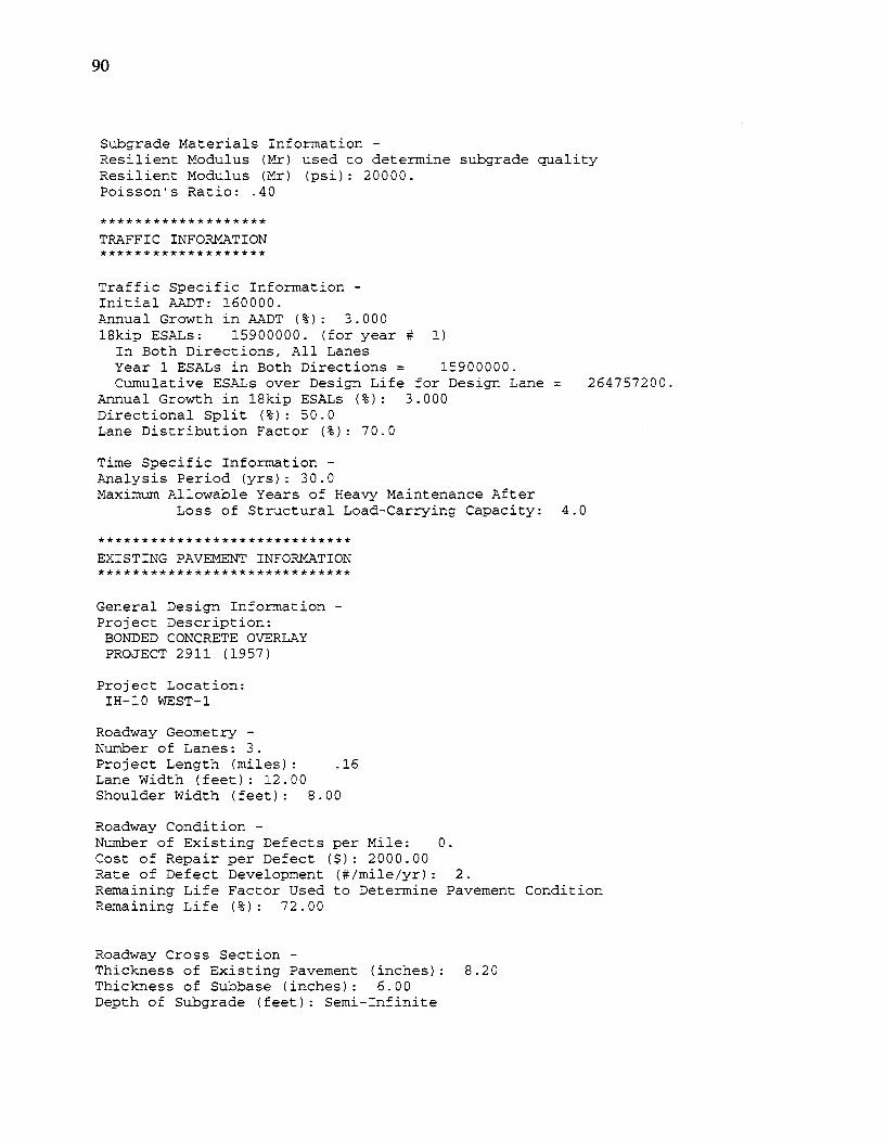
90

Subgrade Materials Information -Resilient Modulus (Mr) used to determine subgrade quality Resilient Modulus (Mr) (psi): 20000. Poisson's Ratio: .40

******************* TRAFFIC INFORMATION *******************

Traffic Specific Information -Initial AADT: 160000. Annual Growth in AADT (%): 3.000 18kip ESALs: 15900000. (for year # 1)

In Both Directions, All Lanes Year 1 ESALs in Both Directions = 15900000. Cumulative ESALs over Design Life for Design Lane = 264757200.

Annual Growth in 18kip ESALs (%): 3.000 Directional Split (%): 50.0 Lane Distribution Factor (%): 70.0

Time Specific Information -Analysis Period (yrs): 30.0 Maximum Allowable Years of Heavy Maintenance After

Loss of Structural Load-Carrying Capacity: 4.0

***************************** EXISTING PAVEMENT INFORMATION *****************************

General Design Information -Project Description:

BONDED CONCRETE OVERLAY PROJECT 2911 (1957)

Project Location: IH-10 WEST-1

Roadway Geometry -Number of Lanes: 3. Project Length (miles): .16 Lane Width (feet): 12.00 Shoulder Width (feet): 8.00

Roadway Condition -Number of Existing Defects per Mile: 0. Cost of Repair per Defect ($): 2000.00 Rate of Defect Development (#/mile/yr): 2. Remaining Life Factor Used to Determine Pavement Condition R~~aining Life (%): 72.00

Roadway Cross Section -Thickness of Existing Pavement (inches): 8.20 Thickness of Subbase (inches): 6.00 Depth of Subgrade (feet): Semi-Infinite

J-Factor Used to Determine Load Transfer Load Transfer Coefficient (J): 2.400 Pavement Type: CRCP Shoulder Type: PCCP Shoulder Load Transfer: Yes

************************ OTHER DESIGN INFORMATION ************************

Reliability (%): 95.000 Initial Serviceability (Po): 4.50 Terminal Serviceability (Pt): 2.50

********************** GEOGRAPHIC INFORMATION **********************

City Name: El Paso

Average Temperatures -January 44.0 February 48.0 March 55.0 April 64.0 May 72.0 June 81.0 July 83.0 August 80.0 September: 74.0 October 64.0 November 51.0 December 44.0

Average Temperature Range -January 28.00 February 29.00 March 29.00 April 30.00 May 30.00 June 30.00 July 25.00 August 25.00 September: 27.00 October 30.00 November 29.00 December 27.00

Solar Radiation -January 440. February 516. March 638. April 784. May 897. June 964.

91

92

July August September: October November December

979. 946. 860. 734. 587. 474.

Wind Speed -January 8. 80 February 9 . 7 0 March April May June July August September: October November December

11.60 11.60 10.90

9.90 8.70 8.20 8.00 7.90 8.20 8.30

Latitude (degrees): 31.800 Longitude (degrees): 106.400 Elevation (feet): 3918

************************ THICKNESS DESIGN RESULTS ************************

1993 AASHTO Design Thickness (inches): 3.8 BCOPRDS Design Thickness {inches): 5.5

************************************************************************ * *

BONDED CONCRETE OVERLAY COMPUTER AIDED DESIGN VERSION 1.0 alpha #2

* *

*======================================================================* * WRITTEN BY * * ROBERT OTTO RASMUSSEN, E.I.T. * * FOR * * THE CENTER FOR TRANSPORTATION RESEARCH * * UNIVERSITY OF TEXAS AT AUSTIN * * AUSTIN, TEXAS * * PROJECT NUMBER 2911 * *======================================================================* ************************************************************************ * PLEASE BE ADVISED THAT NO WARRANTY IS MADE BY TEXAS DEPARTMENT OF * * TRANSPORTATION, CENTER FOR TRANSPORTATION RESEARCH, OR THE AUTHOR(S) * * AS TO THE ACCURACY, COMPLETENESS, RELIABILITY, USABILITY, OR * * SUITABILITY OF THE COMPUTER PROGRAM, ITS DATA, AND DOCUMENTATION. NO * * RESPONSIBILITY IS ASSUMED BY THE ABOVE PARTIES FOR INCORRECT RESULTS * * OR DAMAGES RESULTING FROM THE USE OF THE PROGRAM. * ************************************************************************

********************* MATERIALS INFORMATION *********************

General Materials Information -Standard Deviation: .39 Loss of Subbase Support: .00 Coefficient of Drainage: 1.000

Overlay Materials Information -Modulus of Elasticity (Eol) (psi l : 5000000.

Entered Directly Poisson's Ratio: .15 Flexural Strength (S'c) (psi): 850.

Entered Directly

Existing Pavement Materials Information -Modulus of Elasticity (Epv) (psi): 3500000.

Entered Directly Poisson's Ratio: .15 Flexural Strength (S'c) (psi): 854.

Entered Directly Critical Stress Factor: 1.05 Concrete Stiffness after Cracking (psi): 800000.

Subbase Materials Information -Modulus of Elasticity (Esb) (psi): 100000. Poisson's Ratio: .30

Subgrade Materials Information -Resilient Modulus (MrJ used to determine subgrade quality Resilient Modulus (MrJ (psi): 20000. Poisson's Ratio: .40

******************* TRAFFIC INFORMATION *******************

Traffic Specific Information -Initial AADT: 160000. Annual Growth in AADT (%): 3.000 18kip ESALs: 15900000. (for year # 1)

In Both Directions, All Lanes Year 1 ESALs in Both Directions 15900000. Cumulative ESALs over Design Life for Design Lane 264757200.

Annual Growth in 18kip ESALs (%): 3.000 Directional Split (%): 50.0 Lane Distribution Factor (%): 70.0

Time Specific Information -Analysis Period (yrs): 30.0 Maximum Allowable Years of Heavy Maintenance After

Loss of Structural Load-Carrying Capacity: 4.0

93

94

***************************** EXISTING PAVEMENT INFORMATION *****************************

General Design Information -Project Description:

BONDED CONCRETE OVERLAY PROJECT 2911 (1957)

Project Location: IH-10 WEST-2

Roadway Geometry Number of Lanes: 3. Project Length (miles): .41 Lane Width (feet): 12.00 Shoulder Width (feet): 8.00

Roadway Condition -Number of Existing Defects per Mile: 11. Cost of Repair per Defect ($): 2000.00 Rate of Defect Development (#/mile/yr): 2. Remaining Life Factor Used to Determine Pavement Condition Remaining Life (%): 69.00

Roadway Cross Section -Thickness of Existing Pavement (inches): 8.00 Thickness of Subbase (inches): 6.00 Depth of Subgrade (feet): Semi-Infinite J-Factor Used to Determine Load Transfer Load Transfer Coefficient (J): 2.400 Pavement Type: CRCP Shoulder Type: PCCP Shoulder Load Transfer: Yes

************************ OTHER DESIGN INFORMATION ************************

Reliability (%): 95.000 Initial Serviceability (Po): 4.50 Terminal Serviceability (Pt): 2.50

********************** GEOGRAPHIC INFORMATION **********************

City Name: El Paso

Average Temperatures -January 44.0 February 48.0 March 55.0

April 64.0 May 72.0 June 81.0 July 83.0 August 80.0 September: 7 4 . 0 October 64.0 November 51.0 December 44.0

Average Temperature Range -January 28.00 February 29.00 March 29.00 April 30.00 May 30.00 June 30.00 July 25.00 August 25.00 September: 27.00 October 30.00 November 29.00 December 27.00

Solar Radiation -January 440. February 516. March 638. April 784. May 897. June 964. July 979. August 946. September: 860. October 734. November 587. December 474.

Wind Speed -January 8.80 February 9.70 March 11.60 April 11.60 May 10.90 June 9.90 July 8.70 August 8.20 September: 8.00 October 7.90 November 8.20 December 8.30

Latitude (degrees): 31.800 Longitude (degrees): 106.400 Elevation (feet): 3918

95

96

************************ THICKNESS DESIGN RESULTS ************************

1993 AASHTO Design Thickness (inches): 4.2 BCOPRDS Design Thickness (inches): 6.5

************************************************************************

* *

BONDED CONCRETE OVERLAY COMPUTER AIDED DESIGN VERSION 1.0 alpha #2

* *

*======================================================================* * WRITTEN BY * * ROBERT OTTO RASMUSSEN, E.I.T. * * FOR * * THE CENTER FOR TRANSPORTATION RESEARCH * * UNIVERSITY OF TEXAS AT AUSTIN * * AUSTIN, TEXAS * * PROJECT NUMBER 2911 *

*======================================================================* ************************************************************************ * PLEASE BE ADVISED THAT NO WARRANTY IS MADE BY TEXAS DEPARTMENT OF * * TRANSPORTATION, CENTER FOR TRANSPORTATION RESEARCH, OR THE AUTHOR(Sl * * AS TO THE ACCURACY, COMPLETENESS, RELIABILITY, USABILITY, OR * * SUITABILITY OF THE COMPUTER PROGRAM, ITS DATA, AND DOCUMENTATION. NO * * RESPONSIBILITY IS ASSUMED BY THE ABOVE PARTIES FOR INCORRECT RESULTS * * OR DAMAGES RESULTING FROM THE USE OF THE PROGRAM. * ************************************************************************

********************* MATERIALS INFORMATION *********************

General Materials Information -Standard Deviation: .39 Loss of Subbase Support: .00 Coefficient of Drainage: 1.000

Overlay Materials Information -Modulus of Elasticity (Eol) (psi): 5000000.

Entered Directly Poisson's Ratio: .15 Flexural Strength {S'c) {psi): 850.

Entered Directly

Existing Pavement Materials Information -Modulus of Elasticity (Epv) (psi): 3000000.

Entered Directly Poisson's Ratio: .15 Flexural Strength (S'c) (psi): 854.

Entered Directly Critical Stress Factor: 1.05 Concrete Stiffness after Cracking (psi): 800000.

Subbase Materials Information -Modulus of Elasticity (Esb) (psi): 150000. Poisson's Ratio: .30

Subgrade Materials Information -Resilient Modulus (Mr) used to determine subgrade quality Resilient Modulus (Mr) (psi): 20000. Poisson's Ratio: .40

******************* TRAFFIC INFORMATION *******************

Traffic Specific Information -Initial AADT: 160000. Annual Growth in AADT (%): 3.000 18kip ESALs: 15900000. (for year # 1)

In Both Directions, All Lanes Year 1 ESALs in Both Directions = 15900000. Cumulative ESALs over Design Life for Design Lane

Annual Growth in 18kip ESALs (%): 3.000 Directional Split (%): 50.0 Lane Distribution Factor (%): 70.0

Time Specific Information Analysis Period (yrs): 30.0 Maximum Allowable Years of Heavy Maintenance After

Loss of Structural Load-Carrying Capacity: 4.0

***************************** EXISTING PAVEMENT INFORMATION *****************************

General Design Information -Project Description:

BONDED CONCRETE OVERLAY PROJECT 2911 (1957)

Project Location: IH-10 WEST-3

Roadway Geometry -Number of Lanes: 3. Project Length (miles): .36 Lane Width (feet): 12.00 Shoulder Width (feet): 8.00

Roadway Condition -Number of Existing Defects per Mile: 7. Cost of Repair per Defect ($): 2000.00 Rate of Defect Development (#/mile/yr): 2.

264757200.

Remaining Life Factor Used to Determine Pavement Condition Remaining Life (%): 52.00

97

98

Roadway Cross Section -Thickness of Existing Pavement (inches): 7.50 Thickness of Subbase (inches): 6.00 Depth of Subgrade (feet): Semi-Infinite J-Factor Used to Determine Load Transfer Load Transfer Coefficient (J): 2.400 Pavement Type: CRCP Shoulder Type: PCCP Shoulder Load Transfer: Yes

************************ OTHER DESIGN INFORMATION ************************

Reliability (%): 95.000 Initial Serviceability {Po): 4.50 Terminal Serviceability {Pt): 2.50

********************** GEOGRAPHIC INFORMATION **********************

City Name: El Paso

Average Temperatures -January 44.0 February 48. 0 March 55.0 April 64.0 May 72.0 June 81.0 July 83.0 August 80.0 September: 74.0 October 64.0 November 51.0 December 44.0

Average Temperature Range -January 28.00 February 29.00 March 29.00 April 30.00 May 30.00 June 30.00 July 25.00 August 25.00 September: 27.00 October 30.00 November 29.00 December 27.00

Solar Radiation -January 440.

February March April May June July August September: October November December

Wind Speed -

516. 638. 784. 897. 964. 979. 946. 860. 734. 587. 474.

January 8.80 February 9.70 March 11.60 April 11.60 May 10.90 June 9.90 July 8.70 August 8.20 September: 8.00 October 7.90 November 8.20 December 8.30

Latitude (degrees): 31.800 Longitude (degrees): 106.400 Elevation (feet): 3918

************************ THICKNESS DESIGN RESULTS ************************

1993 AASHTO Design Thickness (inches): 4.7 BCOPRDS Design Thickness (inches): 7.0

************************************************************************ * *

BONDED CONCRETE OVERLAY COMPUTER AIDED DESIGN VERSION 1.0 alpha #2

* *

*======================================================================* * WRITTEN BY * * ROBERT OTTO RASMUSSEN, E.I.T. * * FOR * * THE CENTER FOR TRANSPORTATION RESEARCH * * UNIVERSITY OF TEXAS AT AUSTIN * * AUSTIN, TEXAS * * PROJECT NUMBER 2911 * *======================================================================*

************************************************************************ * PLEASE BE ADVISED THAT NO WARRANTY IS MADE BY TEXAS DEPARTMENT OF * * TRANSPORTATION, CENTER FOR TRANSPORTATION RESEARCH, OR THE AUTHOR(S) * *AS TO THE ACCURACY, COMPLETENESS, RELIABILITY, USABILITY, OR *

99

100

* SUITABILITY OF THE COMPUTER PROGRAM, ITS DATA, AND DOCUMENTATION. NO * * RESPONSIBILITY IS ASSUMED BY THE ABOVE PARTIES FOR INCORRECT RESULTS * * OR DAMAGES RESULTING FROM THE USE OF THE PROGRAM. * ************************************************************************

********************* MATERIALS INFORMATION *********************

General Materials Information -Standard Deviation: .39 Loss of Subbase Support: .00 Coefficient of Drainage: 1.000

Overlay Materials Information -Modulus of Elasticity {Eel) {psi): 5000000.

Entered Directly Poisson's Ratio: .15 Flexural Strength (S'c) (psi): 850.

Entered Directly

Existing Pavement Materials Information -Modulus of Elasticity (Epv) (psi): 3000000.

Entered Directly Poisson's Ratio: .15 Flexural Strength (S'c) (psi): 854.

Entered Directly Critical Stress Factor: 1.05 Concrete Stiffness after Cracking (psi): 800000.

Subbase Materials Information -Modulus of Elasticity (Esb) (psi) : Poisson's Ratio: .30

Subgrade Materials Information -

75000.

Resilient Modulus (Mr) used to determine subgrade quality Resilient Modulus (Mr) (psi): 20000. Poisson's Ratio: .40

******************* TRAFFIC INFORMATION *******************

Traffic Specific Information -Initial AADT: 160000. Annual Growth in AADT (%): 3.000 18kip ESALs: 15900000. (for year # 1)

In Both Directions, All Lanes Year 1 ESALs in Both Directions = 15900000. Cumulative ESALs over Design Life for Design Lane =

Annual Growth in 18kip ESALs (%): 3.000 Directional Split (%): 50.0 Lane Distribution Factor (%): 70.0

Time Specific Information -

264757200.

Analysis Period (yrs): 30.0 Maximum Allowable Years of Heavy Maintenance After

Loss of Structural Load-Carrying Capacity: 4.0

***************************** EXISTING PAVEMENT INFORMATION *****************************

General Design Information -Project Description:

BONDED CONCRETE OVERLAY PROJECT 2911 (1957)

Project Location: IH-10 WEST-4

Roadway Geometry Number of Lanes: 3. Project Length (miles): .25 Lane Width (feet): 12.00 Shoulder Width (feet): 8.00

Roadway Condition -Number of Existing Defects per Mile: 4. Cost of Repair per Defect ($): 2000.00 Rate of Defect Development (#/mile/yr): 2. Remaining Life Factor Used to Determine Pavement Condition Remaining Life (%): 60.00

Roadway Cross Section -Thic~~ess of Existing Pavement (inches): 8.00 Thickness of Subbase (inches): 6.00 Depth of Subgrade (feet): Semi-Infinite J-Factor Used to Determine Load Transfer Load Transfer Coefficient (J): 2.400 Pavement Type: CRCP Shoulder Type: PCCP Shoulder Load Transfer: Yes

************************ OTHER DESIGN INFORMATION ************************

Reliability (%): 95.000 Initial Serviceability (Po): 4.50 Terminal Serviceability (Ptl: 2.50

********************** GEOGRAPHIC INFORMATION **********************

City Name: El Paso

Average Temperatures -

101

102

January February March April May June July August September: October November December

44.0 48.0 55.0 64.0 72.0 81.0 83.0 80.0 74.0 64.0 51.0 44.0

Average Temperature Range -January 28.00 February 29.00 March 29.00 April 30.00 May 30.00 June 30.00 July 25.00 August 25.00 September: 27.00 October 30.00 November 29.00 December 27.00

Solar Radiation -January 440. February 516. March 638. April 784. May 897. June 964. July 979. August 946. September: 860. October 734. November 587. December 474.

Wind Speed -January 8.80 February 9.70 March 11.60 April 11.60 May 10.90 June 9.90 July 8. 70 August 8.20 September: 8.00 October 7.90 November 8.20 December 8 . 3 0

Latitude (degrees): 31.800 Longitude (degrees): 106.400 Elevation (feet): 3918

************************ THICKNESS DESIGN RESULTS ************************

1993 AASHTO Design Thickness (inches): 4.2 BCOPRDS Design Thic~>ess (inches): 6.5

************************************************************************ * *

BONDED CONCRETE OVERLAY COMPUTER AIDED DESIGN VERSION 1.0 alpha #2

* *

*==========~===========================================================* * WRITTEN BY * * ROBERT OTTO RASMUSSEN, E.I.T. * * FOR * * THE CENTER FOR TRANSPORTATION RESEARCH * * UNIVERSITY OF TEXAS AT AUSTIN * * AUSTIN, TEXAS * * PROJECT NUMBER 2911 *

*======================================================================* ************************************************************************ * PLEASE BE ADVISED THAT NO WARRANTY IS MADE BY TEXAS DEPARTMENT OF * * TRANSPORTATION, CENTER FOR TRANSPORTATION RESEARCH, OR THE AUTHOR(S) * * AS TO THE ACCURACY, COMPLETENESS, RELIABILITY, USABILITY, OR * * SUITABILITY OF THE COMPUTER PROGRAM, ITS DATA, AND DOCUMENTATION. NO * * RESPONSIBILITY IS ASSUMED BY THE ABOVE PARTIES FOR INCORRECT RESULTS * * OR DAMAGES RESULTING FROM THE USE OF THE PROGRAM. * ************************************************************************

********************* MATERIALS INFORMATION *********************

General Materials Information -Standard Deviation: .39 Loss of Subbase Support: .00 ~oefficient of Drainage: 1.000

Overlay Materials Information -Modulus of Elasticity (Eol) (psi): 5000000.

Entered Directly Poisson's Ratio: .15 Flexural Strength (S'c} (psi}: 850.

Entered Directly

Existing Pavement Materials Information -Modulus of Elasticity (Epvl (psi): 3000000.

Entered Directly Poisson's Ratio: .15 Flexural Strength (S'c) (psi): 854.

103

104

Entered Directly Critical Stress Factor: 1.05 Concrete Stiffness after Cracking (psi): 800000.

Subbase Materials Information -Modulus of Elasticity (Esb) (psi): Poisson's Ratio: .30

Subgrade Materials Information -

75000.

Resilient Modulus (Mrl used to determine subgrade quality Resilient Modulus (Mr) (psi): 20000. Poisson's Ratio: .40

******************* TRAFFIC INFORMATION *******************

Traffic Specific Information -Initial AADT: 160000. Annual Growth in AADT (%): 3.000 18kip ESALs: 15900000. (for year # 1)

In Both Directions, All Lanes Year 1 ESALs in Both Directions = 15900000. Cumulative ESALs over Design Life for Design Lane = 264757200.

Annual Growth in 18kip ESALs (%): 3.000 Directional Split (%): 50.0 Lane Distribution Factor (%): 70.0

Time Specific Information -Analysis Period (yrs}: 30.0 Maximum Allowable Years of Heavy Maintenance After

Loss of Structural Load-Carrying Capacity: 4.0

***************************** EXISTING PAVEMENT INFORMATION *****************************

General Design Information -Project Description:

BONDED CONCRETE OVERLAY PROJECT 2911 (1957}

Project Location: IH-10 WEST-5

Roadway Geometry -Number of Lanes: 3. Project Length (miles): .34 Lane Width (feet): 12.00 Shoulder Width (feet): 8.00

Roadway Condition -Number of Existing Defects per Mile: 7. Cost of Repair per Defect ($): 2000.00 Rate of Defect Development (#/mile/yr}: 2.

Remaining Life Factor Used to Determine Pavement Condition Remaining Life (%}: 70.00

Roadway Cross Section -Thickness of Existing Pavement (inches}: 8.50 Thickness of Subbase (inches): 6.00 Depth of Subgrade (feet): Semi-Infinite J-Factor Used to Determine Load Transfer Load Transfer Coefficient (J): 2.400 Pavement Type: CRCP Shoulder Type: PCCP Shoulder Load Transfer: Yes

************************ OTHER DESIGN INFORMATION ************************

Reliability (%): 95.000 Initial Serviceability (Po}: 4.50 Terminal Serviceability (Pt): 2.50

********************** GEOGRAPHIC INFORMATION **********************

City Name: El Paso

Average Temperatures January 44.0 February 48.0 March 55.0 April 64.0 May 72.0 June 81.0 July 83.0 August 80.0 September: 74.0 October 64.0 November 51.0 December 44.0

Average Temperature Range January 28.00 February 29.00 March 29.00 April 30.00 May 30.00 June 30.00 July 25.00 August 25.00 September: 27.00 October 30.00 November 29.00 December 27.00

105

106

Solar Radiation -January 440. February 516. March 638. April 784. May 897. June 964. July 979. August 946. September: 860. October 734. November 587. December 474.

Wind Speed -January 8.80 February 9. 7 0 March 11.60 April 11.60 May 10.90 June 9.90 July 8.70 August 8.20 September: 8.00 October 7.90 November 8.20 December 8.30

Latitude (degrees): 31.800 Longitude (degrees): 106.400 Elevation (feet}: 3918

************************ THICKNESS DESIGN RESULTS ************************

1993 AASHTO Design Thickness (inches): 3.6 BCOPRDS Design Thickness (inches): 5.5