170

CHAPTER – 4

STANDARDIZATION OF THE TEACHING

APTITUDE TEST

4.1 Introduction

4.2 Teaching Aptitude Test

4.2.1 Pre-Pilot Test

4.2.1.1 Administration of Pre-Pilot Test

4.2.1.2 Sample

4.2.1.3 Time Limit

4.2.1.4 Method of Scoring

4.2.1.5 Item Analysis

4.2.1.6 Discriminative power

4.2.1.7 Difficulty Index

4.2.2 Pilot Test

4.2.2.1 Selection of Test Items

4.2.2.2 Sample

4.2.2.3 Administration of Pilot Test

4.2.2.4 Element of Time

4.2.2.5 Scoring Scheme

4.2.2.6 Analysis and Interpretation

4.2.3 Final Test

4.2.3.1 Construction of Final Test

171

4.2.3.2 Final Test and Answer sheet

4.2.3.3 Sample for the Final Test

4.2.3.4 Administration of the Final Test

4.2.3.5 Time Limit

4.2.3.6 Scoring the Test

4.3 Establishment of Norms

4.3.1 Difference between the Mean Teaching

Aptitude Scores of Male and Female B.Ed.

Students

4.3.2 Deciding the Nature of the Distribution of

Test Scores

4.3.3 Standard Score and T scores

4.3.4 Percentile Rank

4.4 Reliability of the Test

4.5 Validity of the Test

4.6 Conclusion

172

CHAPTER – 4

STANDARDIZATIONOF THE TEACHING

APTITUDE TEST

4.1 Introduction :

In this chapter the researcher has discussed in detail about the

process of standardization of the tool –Teaching Aptitude Test. The focal

point of this chapter is the reliability and validity of the tool standardized.

The fundamental purpose of standardizing, a psychological test is to

establish its reliability and its validity at as high a level as possible. The

techniques of establishing reliability and validity are discussed in this

chapter. The Norms establishment was the second most important part of

this chapter. To standardize the test the researcher had administered the

tool following the three steps – Pre-Pilot, Pilot, and Final test. The

administration and results of Pre-Pilot Test, Pilot Test and Final Test of

Teaching Aptitude Test are discussed in the beginning of the chapter.

4.2 Teaching Aptitude Test

As discussed in the previous chapter-3: ‘Planning and Procedure of

the Study’, the first two steps to construct the teaching aptitude test was –

Job Analysis and Tentative Selection or Construction of Tests, the rest

of three steps as suggested by Garret1, have been discussed in this

chapter. The steps are as follows:

o EXPERIMENTAL TRYOUT OF THE TEST

o SETTING-UP DIRECTIONS FOR ADMINISTRSTION AND

SCORING; THE ESTABLISHMENT OF NORMS

173

o FOLLOW-UP STUDIES TO DETERMINE THE PREDICTIVE

VALUE OF THE TEST BATTERY IN SELECTION AND IN

VOCATIONAL GUIDANCE

o EXPERIMENTAL TRYOUT OF THE TEST

4.2.1 Pre-Pilot Test

Pre-Pilot Test is considered to be a very important step in the

standardization of a test. Pre-Pilot From of a test has certain basic

objectives, such as

o To identify weak or defective items from a lot.

o To indicate the need of improvement.

o To find out ambiguity from an item and either improve it or

remove it from the test to make it self-explanatory.

o To find out efficiency of the distracters.

o To determine the discriminative power of each item in order so that

all items selected may contribute to central purpose of finished test

and together constitute an efficient measuring instrument.

o To determine difficulty index of each item in order to arrange them

in sequence.

o To find out appropriate time limit for the final form of the test.

o To study efficiency of instructions to examiners and examinee.

The try-out test was planned with a view to these objectives.

4.2.1.1 Administration of Pre-Pilot Test

Pre-Pilot Test was prepared on the basis of teacher’s traits

selected with the help of five point scale. Since this was the first

step in the process of this research, the researcher had administered

174

personally in Four B. Ed. Colleges in Gujarat State. With the help

of this step the researcher could detect ambiguity and otherwise in

the instructions for the test. The researcher had also tried to have an

eye on the time required by average respondents in taking the test

in order to see that the test did not become too lengthy. The

administration of the test personally also helped in knowing if the

test items were ambiguous, too difficult or otherwise since the

proctor had established enough rapport to obtain free reactions

from the respondents.

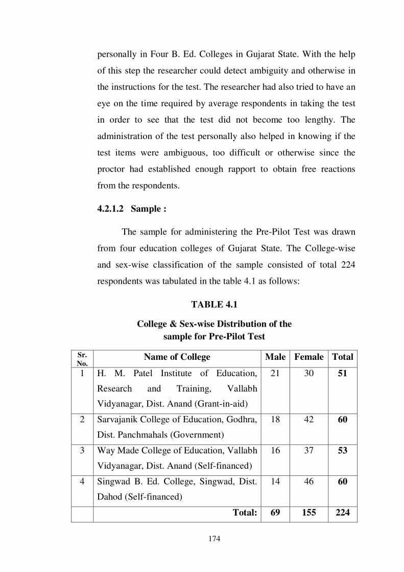
4.2.1.2 Sample :

The sample for administering the Pre-Pilot Test was drawn

from four education colleges of Gujarat State. The College-wise

and sex-wise classification of the sample consisted of total 224

respondents was tabulated in the table 4.1 as follows:

TABLE 4.1

College & Sex-wise Distribution of the

sample for Pre-Pilot Test

Sr.

No. Name of College Male Female Total

1 H. M. Patel Institute of Education,

Research and Training, Vallabh

Vidyanagar, Dist. Anand (Grant-in-aid)

21 30 51

2 Sarvajanik College of Education, Godhra,

Dist. Panchmahals (Government)

18 42 60

3 Way Made College of Education, Vallabh

Vidyanagar, Dist. Anand (Self-financed)

16 37 53

4 Singwad B. Ed. College, Singwad, Dist.

Dahod (Self-financed)

14 46 60

Total: 69 155 224

175

From the table 4.1 it can be seen that on an average 50 to 60

students were selected from each four colleges. The Pre-Pilot Test

was administered in the first term i.e. in the month of August of the

academic year 2010-2011.

4.2.1.3 Time Limit

This test was a power test. Anastasi2 defines power test in the

following words :

“A pure power test has a time limit long enough to permit

everyone to attempt all items.”

According to Gilford3;

“A power test is often defined as one in which every

examinee has a chance to attempt every item.”

Keeping these definitions in mind, no time limit was fixed

for the Pre-Pilot Test. Respondents were informed that they would

have as much time as they needed for the completion of this test.

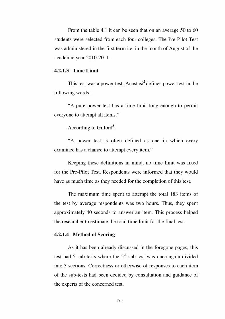
The maximum time spent to attempt the total 183 items of

the test by average respondents was two hours. Thus, they spent

approximately 40 seconds to answer an item. This process helped

the researcher to estimate the total time limit for the final test.

4.2.1.4 Method of Scoring

As it has been already discussed in the foregone pages, this

test had 5 sub-tests where the 5th

sub-test was once again divided

into 3 sections. Correctness or otherwise of responses to each item

of the sub-tests had been decided by consultation and guidance of

the experts of the concerned test.

176

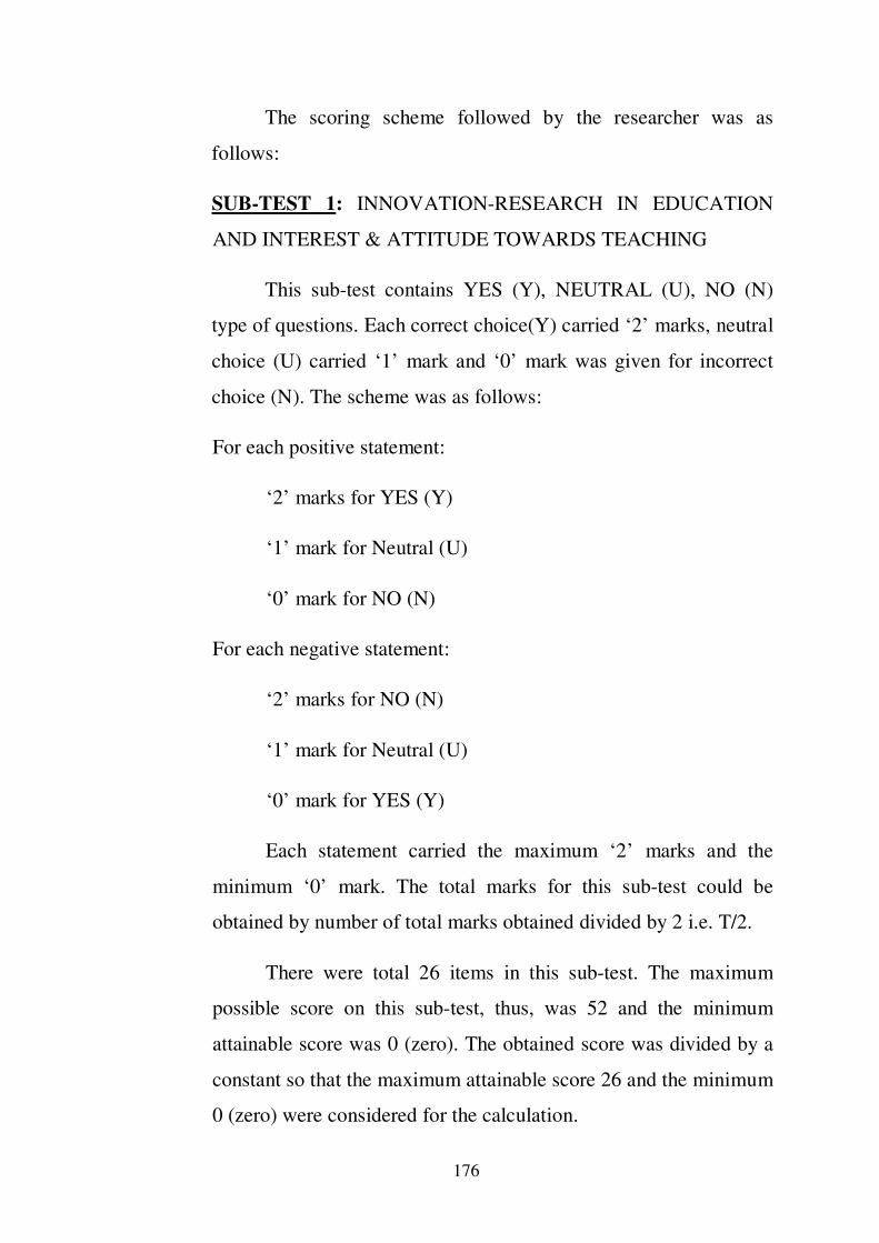
The scoring scheme followed by the researcher was as

follows:

SUB-TEST 1: INNOVATION-RESEARCH IN EDUCATION

AND INTEREST & ATTITUDE TOWARDS TEACHING

This sub-test contains YES (Y), NEUTRAL (U), NO (N)

type of questions. Each correct choice(Y) carried ‘2’ marks, neutral

choice (U) carried ‘1’ mark and ‘0’ mark was given for incorrect

choice (N). The scheme was as follows:

For each positive statement:

‘2’ marks for YES (Y)

‘1’ mark for Neutral (U)

‘0’ mark for NO (N)

For each negative statement:

‘2’ marks for NO (N)

‘1’ mark for Neutral (U)

‘0’ mark for YES (Y)

Each statement carried the maximum ‘2’ marks and the

minimum ‘0’ mark. The total marks for this sub-test could be

obtained by number of total marks obtained divided by 2 i.e. T/2.

There were total 26 items in this sub-test. The maximum

possible score on this sub-test, thus, was 52 and the minimum

attainable score was 0 (zero). The obtained score was divided by a

constant so that the maximum attainable score 26 and the minimum

0 (zero) were considered for the calculation.

177

SUB-TEST II: TEACHER’S EXCELLENCY IN SUBJECT-

CONTENT, TEACHING METHODS AND EVALUATION IN

EDUCATION

This sub-test contains multiple choice types of questions. It

had four alternative choices A, B, C, D, respectively for each item.

Each correct choice carried ‘1’ mark and ‘0’ mark was given for

any other choice. The maximum and the minimum possible score

on this sub-test was ‘39’ and ‘0’ respectively.

SUB-TEST III: TEACHER’S COMMITMENT

This sub-test contains the same types of questions as in sub-

test I. The maximum possible score on this sub test was ‘27’ and

the minimum was ‘0’.

SUB-TEST IV: TEACHER’S HUMAN RELATIONSHIPS AND

SOCIAL ACCOUNTABILITY

This sub test contains a 5 point scale.

For each positive statement,

‘4’ marks for Fully Agree (SA)

‘3’ marks for Agree (A)

‘2’ marks for Neutral (U)

‘1’ mark for Disagree (D)

‘0’ mark for Fully Disagree (SD)

For each negative statement,

‘4’ marks for Fully Disagree (SD)

‘3’ marks for Disagree (D)

178

‘2’ marks for Neutral (U)

‘1’ mark for Agree (A)

‘0’ mark for Fully Agree (SA)

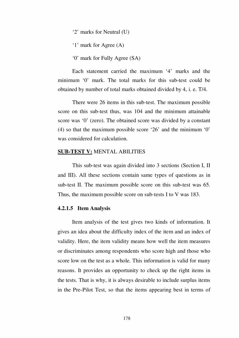
Each statement carried the maximum ‘4’ marks and the

minimum ‘0’ mark. The total marks for this sub-test could be

obtained by number of total marks obtained divided by 4, i. e. T/4.

There were 26 items in this sub-test. The maximum possible

score on this sub-test thus, was 104 and the minimum attainable

score was ‘0’ (zero). The obtained score was divided by a constant

(4) so that the maximum possible score ‘26’ and the minimum ‘0’

was considered for calculation.

SUB-TEST V: MENTAL ABILITIES

This sub-test was again divided into 3 sections (Section I, II

and III). All these sections contain same types of questions as in

sub-test II. The maximum possible score on this sub-test was 65.

Thus, the maximum possible score on sub-tests I to V was 183.

4.2.1.5 Item Analysis

Item analysis of the test gives two kinds of information. It

gives an idea about the difficulty index of the item and an index of

validity. Here, the item validity means how well the item measures

or discriminates among respondents who score high and those who

score low on the test as a whole. This information is valid for many

reasons. It provides an opportunity to check up the right items in

the tests. That is why, it is always desirable to include surplus items

in the Pre-Pilot Test, so that the items appearing best in terms of

179

item statistics, can be selected for the try out and final form of the

test.

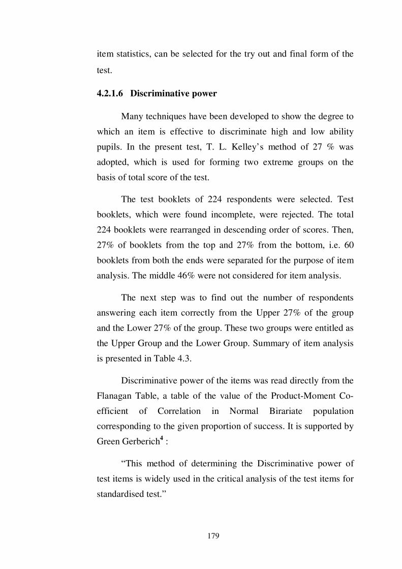
4.2.1.6 Discriminative power

Many techniques have been developed to show the degree to

which an item is effective to discriminate high and low ability

pupils. In the present test, T. L. Kelley’s method of 27 % was

adopted, which is used for forming two extreme groups on the

basis of total score of the test.

The test booklets of 224 respondents were selected. Test

booklets, which were found incomplete, were rejected. The total

224 booklets were rearranged in descending order of scores. Then,

27% of booklets from the top and 27% from the bottom, i.e. 60

booklets from both the ends were separated for the purpose of item

analysis. The middle 46% were not considered for item analysis.

The next step was to find out the number of respondents

answering each item correctly from the Upper 27% of the group

and the Lower 27% of the group. These two groups were entitled as

the Upper Group and the Lower Group. Summary of item analysis

is presented in Table 4.3.

Discriminative power of the items was read directly from the

Flanagan Table, a table of the value of the Product-Moment Co-

efficient of Correlation in Normal Birariate population

corresponding to the given proportion of success. It is supported by

Green Gerberich4 :

“This method of determining the Discriminative power of

test items is widely used in the critical analysis of the test items for

standardised test.”

180

4.2.1.7 Difficulty Index

In the test construction, it is a common practice to attempt to

construct items covering a wide range of difficulty. According to

Green Gerberich5,

“The test as whole should have about 50% difficulty for

average pupils.”

Therefore, items should not be so easy as to be passed by

every participant of the group nor it should be too difficult so as to

be failed by every participant of the group, because neither of these

extreme cases makes the item contribute to the discrimination

which the test is to make among different individuals.

Difficulty values or indices of the items of the present test

were determined by using the data obtained from 27% of each of

the upper and lower groups. For this, the percentages of

respondents answering the items correctly from the upper group

and from the lower group were added and the sum was divided by

2 (two).

The same is mentioned below symbolically along with

illustrations:

Difficulty Index (DI) = (Upper Group + Lower Group)/2

Illustration: Test I : Item 1. DI = (82 + 42) / 2 = 62

Test II : Item 1. DI = (72 + 35) / 2 = 53

In this way, the difficulty index of each item was computed.

The Table 4.2 shows the number of respondents from Upper group

and Lower group answering each item correctly, difficulty index

and discriminative value of the Pre-Pilot Test. An item retained or

rejected was also shown in the last column of the table.

181

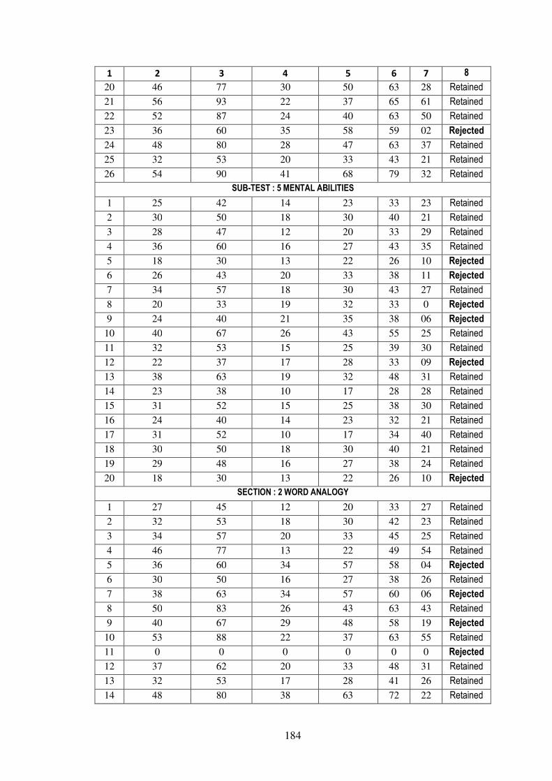
TABLE 4.2

No. of Respondents from Upper and Lower Group answering each

item correctly. The Difficulty Index and Discriminative

Value of the Pre-Pilot Test

ITEM

NO.

(Rh)

UPPER GROUP

NO. OF

CORRECT

RESPONCES

% OF

CORRECT

RESPONCES

R1

LOWER

GROUP NO.

OF CORRECT

RESPONCES

% OF

CORRECT

RESP0NCES

DIF

FIC

ULTY

IND

EX

DIS

CR

IMIN

ATIV

E

VA

LU

E

REMARKS

1 2 3 4 5 6 7 8

SUB-TEST : 1 INNOVATION-RESEARCH IN EDUCATION AND INTEREST AND ATTITUDE TOWARDS

TEACHING 1 49 82 25 42 62 43 Retained

2 34 57 15 25 41 34 Retained

3 38 63 22 37 50 27 Retained

4 47 78 34 57 68 25 Retained

5 25 42 21 35 38 09 Rejected

6 59 98 23 38 68 73 Retained

7 52 87 19 32 59 56 Retained

8 36 60 30 50 55 10 Rejected

9 42 70 24 40 55 31 Retained

10 50 83 37 62 73 25 Retained

11 46 77 13 22 49 54 Retained

12 48 80 18 30 55 51 Retained

13 28 47 26 43 45 04 Rejected

14 30 50 27 45 48 06 Rejected

15 51 85 29 48 67 40 Retained

16 55 92 30 50 71 53 Retained

17 48 80 37 62 71 22 Retained

18 40 67 28 47 57 21 Retained

19 44 73 16 27 50 46 Retained

20 47 78 22 37 58 41 Retained

21 57 95 25 42 68 61 Retained

22 56 93 18 30 62 65 Retained

23 50 83 28 47 65 39 Retained

24 38 63 18 30 47 33 Retained

25 48 80 24 40 60 42 Retained

26 36 60 22 37 48 25 Retained

SUB-TEST: 2 TEACHER’S MASTARY IN SUBJECT-CONTENT, TEACHING METHODS AND EVALUATION IN

EDUCATION

1 43 72 21 35 53 39 Retained

182

1 2 3 4 5 6 7 8

2 23 38 19 32 35 07 Rejected

3 25 42 13 22 32 23 Retained

4 43 72 27 45 58 29 Retained

5 32 53 15 25 39 30 Retained

6 40 67 29 48 58 19 Rejected

7 44 73 30 50 62 23 Retained

8 35 58 14 23 41 38 Retained

9 25 42 16 27 34 18 Rejected

10 39 65 22 37 51 29 Retained

11 27 45 14 23 34 25 Retained

12 26 43 34 57 50 -14 Rejected

13 45 75 29 48 62 28 Retained

14 42 70 27 45 58 27 Retained

15 52 87 10 17 52 68 Retained

16 36 60 22 37 48 25 Retained

17 46 77 26 43 60 36 Retained

18 53 88 33 55 72 41 Retained

19 50 83 18 30 57 53 Retained

20 35 58 25 42 50 16 Rejected

21 43 72 13 22 47 50 Retained

22 38 63 20 33 48 31 Retained

23 47 78 31 52 65 29 Retained

24 28 47 37 62 54 -16 Rejected

25 44 73 26 43 58 31 Retained

26 37 62 22 37 49 27 Retained

27 49 82 19 32 57 51 Retained

28 55 92 16 27 59 68 Retained

29 36 60 24 40 50 21 Retained

30 39 65 29 48 57 17 Rejected

31 40 67 23 38 53 29 Retained

32 42 70 25 42 56 29 Retained

33 34 57 17 28 43 29 Retained

34 31 52 14 23 38 33 Retained

35 35 58 20 33 46 27 Retained

36 30 50 17 28 39 23 Retained

37 53 88 18 30 59 60 Retained

38 38 63 21 35 49 29 Retained

39 47 78 32 53 66 29 Retained

SUB-TEST : 3 TEACHER'S COMMITMENT

1 52 87 38 63 75 31 Retained

2 45 75 35 58 67 18 Rejected

3 55 92 40 67 79 38 Retained

4 25 42 28 47 44 -04 Rejected

183

1 2 3 4 5 6 7 8

5 42 70 25 42 56 29 Retained

6 54 90 43 72 81 28 Retained

7 44 73 22 37 55 37 Retained

8 48 80 29 48 64 35 Retained

9 49 82 36 60 71 27 Retained

10 51 85 40 67 76 24 Retained

11 39 65 21 35 50 31 Retained

12 35 58 16 27 43 33 Retained

13 28 47 18 30 38 17 Rejected

14 38 63 24 40 52 22 Retained

15 40 67 26 43 55 25 Retained

16 56 93 42 70 82 35 Retained

17 39 65 20 33 49 31 Retained

18 45 75 28 47 61 30 Retained

19 53 88 38 63 76 34 Retained

20 58 97 46 77 87 40 Retained

21 35 58 19 32 45 27 Retained

22 49 82 38 63 73 25 Retained

23 53 88 43 72 80 24 Retained

24 56 93 40 67 80 38 Retained

25 51 85 32 53 69 37 Retained

26 38 63 28 47 55 16 Rejected

27 48 80 36 60 70 24 Retained

SUB-TEST : 4 TEACHER'S HUMAN RELATIONSHIPS AND SOCIAL DEDICATION

1 46 77 33 55 66 24 Retained

2 36 60 26 43 52 18 Rejected

3 40 67 22 37 52 31 Retained

4 37 62 18 30 46 33 Retained

5 47 78 28 47 63 34 Retained

6 49 82 36 60 71 27 Retained

7 48 80 30 50 65 33 Retained

8 30 50 20 33 42 19 Rejected

9 50 83 32 53 68 34 Retained

10 49 82 26 43 63 43 Retained

11 53 88 30 50 69 45 Retained

12 42 70 25 42 56 29 Retained

13 46 77 19 32 54 45 Retained

14 34 57 20 33 45 25 Retained

15 52 87 38 63 75 32 Retained

16 50 83 37 62 73 25 Retained

17 46 77 32 53 65 26 Retained

18 38 63 36 60 62 02 Rejected

19 40 67 27 45 56 23 Retained

184

1 2 3 4 5 6 7 8

20 46 77 30 50 63 28 Retained

21 56 93 22 37 65 61 Retained

22 52 87 24 40 63 50 Retained

23 36 60 35 58 59 02 Rejected

24 48 80 28 47 63 37 Retained

25 32 53 20 33 43 21 Retained

26 54 90 41 68 79 32 Retained

SUB-TEST : 5 MENTAL ABILITIES

1 25 42 14 23 33 23 Retained

2 30 50 18 30 40 21 Retained

3 28 47 12 20 33 29 Retained

4 36 60 16 27 43 35 Retained

5 18 30 13 22 26 10 Rejected

6 26 43 20 33 38 11 Rejected

7 34 57 18 30 43 27 Retained

8 20 33 19 32 33 0 Rejected

9 24 40 21 35 38 06 Rejected

10 40 67 26 43 55 25 Retained

11 32 53 15 25 39 30 Retained

12 22 37 17 28 33 09 Rejected

13 38 63 19 32 48 31 Retained

14 23 38 10 17 28 28 Retained

15 31 52 15 25 38 30 Retained

16 24 40 14 23 32 21 Retained

17 31 52 10 17 34 40 Retained

18 30 50 18 30 40 21 Retained

19 29 48 16 27 38 24 Retained

20 18 30 13 22 26 10 Rejected

SECTION : 2 WORD ANALOGY

1 27 45 12 20 33 27 Retained

2 32 53 18 30 42 23 Retained

3 34 57 20 33 45 25 Retained

4 46 77 13 22 49 54 Retained

5 36 60 34 57 58 04 Rejected

6 30 50 16 27 38 26 Retained

7 38 63 34 57 60 06 Rejected

8 50 83 26 43 63 43 Retained

9 40 67 29 48 58 19 Rejected

10 53 88 22 37 63 55 Retained

11 0 0 0 0 0 0 Rejected

12 37 62 20 33 48 31 Retained

13 32 53 17 28 41 26 Retained

14 48 80 38 63 72 22 Retained

185

1 2 3 4 5 6 7 8

15 36 60 20 33 47 29 Retained

16 24 40 18 30 35 11 Rejected

17 43 72 29 48 60 26 Retained

18 49 82 20 33 58 51 Retained

19 45 75 19 32 53 42 Retained

20 35 58 21 35 47 25 Retained

21 47 78 28 47 63 34 Retained

SECTION : 3 WORD RELATION

1 40 67 22 37 52 31 Retained

2 32 53 28 47 50 06 Rejected

3 36 60 18 30 45 31 Retained

4 32 53 16 27 40 28 Retained

5 38 63 20 33 48 31 Retained

6 42 70 24 40 55 31 Retained

7 20 33 17 28 31 04 Rejected

8 37 62 23 38 50 25 Retained

9 46 77 34 57 67 22 Retained

10 50 83 36 60 72 27 Retained

11 52 87 42 70 78 22 Retained

12 36 60 32 53 57 08 Rejected

13 42 70 30 50 60 21 Retained

14 34 57 22 37 47 21 Retained

15 38 63 29 48 56 15 Rejected

16 42 70 28 47 58 25 Retained

17 39 65 21 35 50 31 Retained

18 44 73 20 33 53 40 Retained

19 32 53 30 50 52 02 Rejected

20 46 77 34 57 67 22 Retained

21 33 55 20 33 44 23 Retained

22 39 65 32 53 59 13 Rejected

23 45 75 30 50 63 26 Retained

24 34 57 28 47 52 08 Rejected

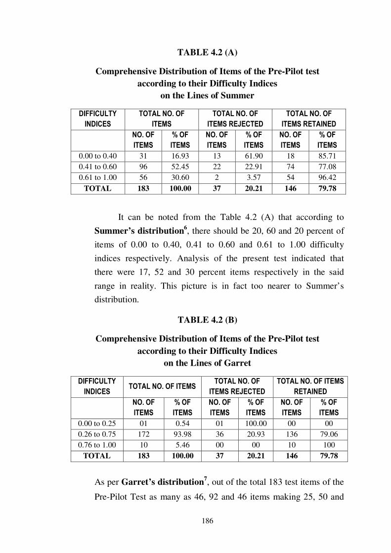
Distribution of grouping of the items of the pre-pilot form of

the test in relation to their difficulty indices, as shown in the above

mentioned table 4.2, it can be well summarized and read from the

comprehensive table 4.2 (A) given below :

186

TABLE 4.2 (A)

Comprehensive Distribution of Items of the Pre-Pilot test

according to their Difficulty Indices

on the Lines of Summer

DIFFICULTY

INDICES

TOTAL NO. OF

ITEMS

TOTAL NO. OF

ITEMS REJECTED

TOTAL NO. OF

ITEMS RETAINED

NO. OF

ITEMS

% OF

ITEMS

NO. OF

ITEMS

% OF

ITEMS

NO. OF

ITEMS

% OF

ITEMS

0.00 to 0.40 31 16.93 13 61.90 18 85.71

0.41 to 0.60 96 52.45 22 22.91 74 77.08

0.61 to 1.00 56 30.60 2 3.57 54 96.42

TOTAL 183 100.00 37 20.21 146 79.78

It can be noted from the Table 4.2 (A) that according to

Summer’s distribution6, there should be 20, 60 and 20 percent of

items of 0.00 to 0.40, 0.41 to 0.60 and 0.61 to 1.00 difficulty

indices respectively. Analysis of the present test indicated that

there were 17, 52 and 30 percent items respectively in the said

range in reality. This picture is in fact too nearer to Summer’s

distribution.

TABLE 4.2 (B)

Comprehensive Distribution of Items of the Pre-Pilot test

according to their Difficulty Indices

on the Lines of Garret

DIFFICULTY

INDICES TOTAL NO. OF ITEMS

TOTAL NO. OF

ITEMS REJECTED

TOTAL NO. OF ITEMS

RETAINED

NO. OF

ITEMS

% OF

ITEMS

NO. OF

ITEMS

% OF

ITEMS

NO. OF

ITEMS

% OF

ITEMS

0.00 to 0.25 01 0.54 01 100.00 00 00

0.26 to 0.75 172 93.98 36 20.93 136 79.06

0.76 to 1.00 10 5.46 00 00 10 100

TOTAL 183 100.00 37 20.21 146 79.78

As per Garret’s distribution7, out of the total 183 test items of the

Pre-Pilot Test as many as 46, 92 and 46 items making 25, 50 and

187

25 percentage respectively of the total should fall in the range of

0.00 to 0.25, 0.26 to 0.75 and 0.76 to 1.00 difficulty indices

respectively. As per the present Pre-Pilot Test, there have been 01,

172 and 10 items making 100, 20.93 and 0 percentages of the total

183 items falling in the range of 0.00 to 0.25, 0.26 to 0.75 and 0.76

to 1.00 difficulty indices respectively. The data indicate an obvious

contrast with Garrett’s distribution and comparatively near to

Summer’s distribution. The reason of this contrast lies in the

selection or rejection of test items. The items of the Pre-Pilot Test

of the test under report have been rejected or retained for the pilot

form of the test not on the basis of their difficulty indices but on the

basis of their discriminating values.

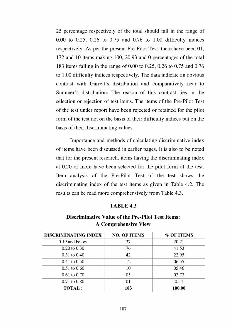
Importance and methods of calculating discriminative index

of items have been discussed in earlier pages. It is also to be noted

that for the present research, items having the discriminating index

at 0.20 or more have been selected for the pilot form of the test.

Item analysis of the Pre-Pilot Test of the test shows the

discriminating index of the test items as given in Table 4.2. The

results can be read more comprehensively from Table 4.3.

TABLE 4.3

Discriminative Value of the Pre-Pilot Test Items:

A Comprehensive View

DISCRIMINATING INDEX NO. OF ITEMS % OF ITEMS

0.19 and below 37 20.21

0.20 to 0.30 76 41.53

0.31 to 0.40 42 22.95

0.41 to 0.50 12 06.55

0.51 to 0.60 10 05.46

0.61 to 0.70 05 02.73

0.71 to 0.80 01 0.54

TOTAL : 183 100.00

188

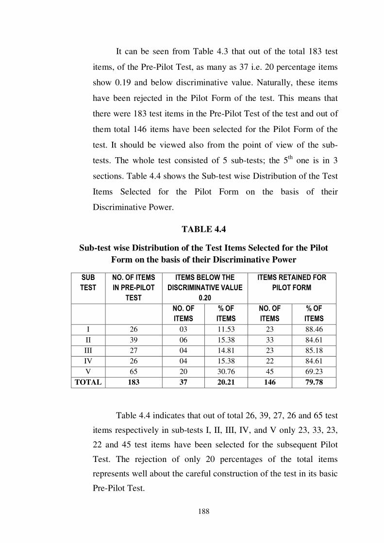
It can be seen from Table 4.3 that out of the total 183 test

items, of the Pre-Pilot Test, as many as 37 i.e. 20 percentage items

show 0.19 and below discriminative value. Naturally, these items

have been rejected in the Pilot Form of the test. This means that

there were 183 test items in the Pre-Pilot Test of the test and out of

them total 146 items have been selected for the Pilot Form of the

test. It should be viewed also from the point of view of the sub-

tests. The whole test consisted of 5 sub-tests; the 5th

one is in 3

sections. Table 4.4 shows the Sub-test wise Distribution of the Test

Items Selected for the Pilot Form on the basis of their

Discriminative Power.

TABLE 4.4

Sub-test wise Distribution of the Test Items Selected for the Pilot

Form on the basis of their Discriminative Power

SUB

TEST

NO. OF ITEMS

IN PRE-PILOT

TEST

ITEMS BELOW THE

DISCRIMINATIVE VALUE

0.20

ITEMS RETAINED FOR

PILOT FORM

NO. OF

ITEMS

% OF

ITEMS

NO. OF

ITEMS

% OF

ITEMS

I 26 03 11.53 23 88.46

II 39 06 15.38 33 84.61

III 27 04 14.81 23 85.18

IV 26 04 15.38 22 84.61

V 65 20 30.76 45 69.23

TOTAL 183 37 20.21 146 79.78

Table 4.4 indicates that out of total 26, 39, 27, 26 and 65 test

items respectively in sub-tests I, II, III, IV, and V only 23, 33, 23,

22 and 45 test items have been selected for the subsequent Pilot

Test. The rejection of only 20 percentages of the total items

represents well about the careful construction of the test in its basic

Pre-Pilot Test.

189

4.2.2 Pilot Test :

The pilot form of the test was constructed as per the Pre-Pilot Test.

4.2.2.1 Selection of the test Items :

Construction of the test items were already scrutinised at the

Pre-Pilot stage. Items found to be ambiguous were modified and

those items showing discriminating indices below 0.20 were

rejected. This gave the final form to the items of the Pilot test.

4.2.2.2 Sample :

The Pilot Form of the test was administered on a total

sample of 500 trainees of B. Ed. Colleges of Gujarat. Details

regarding the number of participants and institutions selected for

the Pilot Form were shown in Table 4.5 as follows:

TABLE 4.5

College & Sex-wise Distribution of the sample for Pilot Test

Sr.

No Name of College Male Female Total

1 Lalitaba Edu. Trust Sanchit B.Ed. College,

Modasa. 25 25 50

2 Shree G. H. Patel College of Education, Patan. 25 25 50

3 M. B. Patel College of Education , Sardar Patel

University, Vallabh Vidyanagar .

50 50 100

4 Shree Vestabhai H. Patel College of B.Ed. (Girls),

Dharampur, Dist. Valsad

25 25 50

5 Smt. S.B. Gardi B.Ed. College, Kharva Road, Opp.

Ramroti Ashram At. Dhrol. Dist. Jamnagar. 25 25 50

6 Christian College of Education I. P. Mission

Compound, Anand

25 25 50

7 College of Education, Shree Satyanarayan Temple

Campus, Kathiria, Nani Daman 25 25 50

Total: 200 200 400

190

From table 4.5 it can be seen that out of the administered

sample of 500, only 400 respondents were found to be proper as

per the instructions and rest of others were discarded either due to

incomplete answer sheets or due to improper indication of answers

in the answer sheets. The pilot test was thus administered on a

sample of 400 trainees.

4.2.2.3 Administration of Pilot Test

It is needless to mention that personal presence of the

researcher at the time of administration of the pilot test helped a lot

in establishing rapport with the respondents to know the

approximate time required for the Final Form of the test as well as

to have clarifications regarding the instructions and the test items.

It was found necessary to specify that all items were not in one and

the same order viz. addition, subtractions etc., but each item had a

different order. No supplementary instructions or specifications

were required in any other sub-tests. An overall check-up was

needed at the end to see if any test item was left unanswered by any

respondent. There were instances when some trainees were

required to mark their answers to the test items which they had left

unanswered. Indeed, such instances were only casual.

4.2.2.4 Element of Time

This was not a speed test. Hence, the respondents could take

as much time as they needed to answer each items of the test. The

overall time estimated in taking the entire pilot test was around 95

191

minutes. It was thought that one item would take about 45 seconds

in general, but the items of the sub-test V were having the element

of mathematical calculations, would naturally take some more

time. Hence, the sub-test V would take 15 minutes more in addition

to the total time required. Of course, this was only for the

consideration of the researcher and the respondents were not

informed in this regard. But practical administration of the Pilot

Form of the test took 90 minutes.

4.2.2.5 Scoring Scheme

The test items for the Pilot Form of the test were drawn from

the Pre Tyr-out Form of the test with necessary modifications in

construction of the statements. But there was no change in the form

of the test and sub-tests. There was a minor change in the form of

order of statements and increase/decrease of negative statements.

Hence, the scoring scheme for this Pilot Form of the test remained

the same as that of the Pre-Pilot Test. The total score of the Pilot

test accordingly was 146.

4.2.2.6 Analysis and Interpretation of Results

The answer sheets were assessed according to the scoring

scheme after the administration of the Pilot Form of the test. The

total answer sheets were rearranged in ascending order as 1 to 400.

The one who got the highest score was numbered at 1 and

respectively all others were numbered as per their score and the

lowest score was numbered 400 (the last). The higher and the lower

192

groups were formed as per the scheme mentioned in Pre-Pilot Form

of the test.

The higher group consisted of 27% (i.e.108) highest

achieved score and the lowest group consisted of 27% (i.e.108)

lowest achieved score. This means the answer sheet no. 1 to 108

formed the Upper Group and that answer sheet no. 292 to 400

formed the Lower Group. The number of those respondents who

answered each item correctly was found from each of the two

groups. This is shown in Table 4.6. There were 108 respondents in

each of the two groups. The percentage of the Upper Group (Rh)

and the Lower Group (R1) for each item had also been shown in

the Table 4.6.

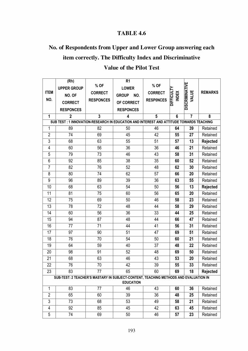
Discriminative value of each statement was calculated by

using the Flanagan Table as given in the book: Statistical Inference

Helen M. Walker and Joseph Lev (1965)8. Difficulty index of each

statement was drawn by using the procedure as discussed earlier

(4.2.2.7) of this chapter. Table 4.6 shows group-wise number and

percentage of correct responses, difficulty index and discriminative

value of each item of the Pilot Form of the Test. Items retained or

rejected is also shown in the last column of the table.

193

TABLE 4.6

No. of Respondents from Upper and Lower Group answering each

item correctly. The Difficulty Index and Discriminative

Value of the Pilot Test

ITEM

NO.

(Rh)

UPPER GROUP

NO. OF

CORRECT

RESPONCES

% OF

CORRECT

RESPONCES

R1

LOWER

GROUP NO.

OF CORRECT

RESPONCES

% OF

CORRECT

RESP0NCES

DIF

FIC

ULTY

IND

EX

DIS

CR

IMIN

ATIV

E

VA

LU

E

REMARKS

1 2 3 4 5 6 7 8 SUB TEST : 1 INNOVATION-RESEARCH IN EDUCATION AND INTEREST AND ATTITUDE TOWARDS TEACHING

1 89 82 50 46 64 39 Retained

2 74 69 45 42 55 27 Retained

3 68 63 55 51 57 13 Rejected

4 60 56 36 36 46 21 Retained

5 79 73 46 43 58 31 Retained

6 92 85 38 35 60 52 Retained

7 82 76 52 48 62 30 Retained

8 80 74 62 57 66 20 Retained

9 96 89 39 36 63 55 Retained

10 68 63 54 50 56 13 Rejected

11 81 75 60 56 65 20 Retained

12 75 69 50 46 58 23 Retained

13 78 72 48 44 58 29 Retained

14 60 56 36 33 44 25 Retained

15 94 87 48 44 66 47 Retained

16 77 71 44 41 56 31 Retained

17 97 90 51 47 69 51 Retained

18 76 70 54 50 60 21 Retained

19 64 59 40 37 48 22 Retained

20 98 91 52 48 69 50 Retained

21 68 63 46 43 53 20 Retained

22 76 70 42 39 55 33 Retained

23 83 77 65 60 69 18 Rejected

SUB-TEST: 2 TEACHER’S MASTARY IN SUBJECT-CONTENT, TEACHING METHODS AND EVALUATION IN

EDUCATION

1 83 77 46 43 60 36 Retained

2 65 60 39 36 48 25 Retained

3 73 68 53 49 58 21 Retained

4 92 85 45 42 63 45 Retained

5 74 69 50 46 57 23 Retained

194

1 2 3 4 5 6 7 8

6 65 60 66 61 61 13 Rejected

7 79 73 42 39 56 22 Retained

8 87 81 48 44 63 39 Retained

9 95 88 59 55 71 41 Retained

10 82 76 64 59 68 20 Retained

11 62 57 38 35 46 23 Retained

12 66 61 42 39 50 22 Retained

13 84 78 52 48 63 33 Retained

14 93 86 66 61 74 33 Retained

15 70 65 46 43 54 22 Retained

16 94 87 44 41 64 50 Retained

17 98 91 60 56 73 43 Retained

18 87 81 68 63 72 22 Retained

19 77 71 51 47 59 25 Retained

20 97 90 43 40 65 56 Retained

21 69 64 50 46 55 19 Rejected

22 47 44 48 44 44 0 Rejected

23 66 61 40 37 49 25 Retained

24 60 56 36 33 44 25 Retained

25 72 67 50 46 56 21 Retained

26 71 66 46 43 54 25 Retained

27 64 59 51 47 53 12 Rejected

28 80 74 53 49 62 28 Retained

29 75 69 62 57 63 15 Rejected

30 93 86 55 51 69 42 Retained

31 88 81 67 62 72 22 Retained

32 76 70 54 50 60 21 Retained

33 70 65 50 46 56 19 Rejected

SUB TEST : 3 TEACHER'S COMMITMENT

1 104 96 70 65 81 51 Retained

2 97 90 86 80 85 18 Rejected

3 84 78 50 46 62 34 Retained

4 98 91 68 63 77 38 Retained

5 88 81 44 41 61 42 Retained

6 86 80 72 67 73 17 Rejected

7 89 82 72 67 75 20 Retained

8 74 69 62 57 63 13 Rejected

9 79 73 52 48 61 26 Retained

10 85 79 51 47 63 34 Retained

11 78 72 54 50 61 23 Retained

12 80 74 57 53 63 24 Retained

13 75 69 48 44 57 25 Retained

14 79 73 46 43 58 31 Retained

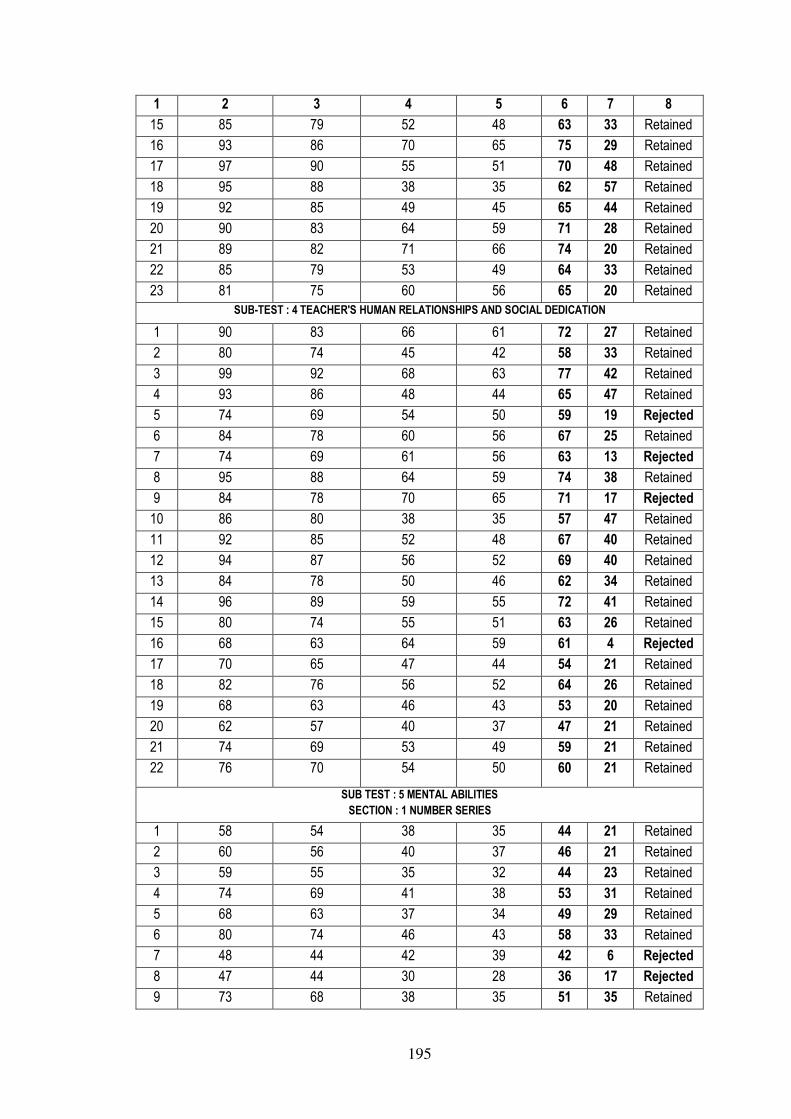
195

1 2 3 4 5 6 7 8

15 85 79 52 48 63 33 Retained

16 93 86 70 65 75 29 Retained

17 97 90 55 51 70 48 Retained

18 95 88 38 35 62 57 Retained

19 92 85 49 45 65 44 Retained

20 90 83 64 59 71 28 Retained

21 89 82 71 66 74 20 Retained

22 85 79 53 49 64 33 Retained

23 81 75 60 56 65 20 Retained

SUB-TEST : 4 TEACHER'S HUMAN RELATIONSHIPS AND SOCIAL DEDICATION

1 90 83 66 61 72 27 Retained

2 80 74 45 42 58 33 Retained

3 99 92 68 63 77 42 Retained

4 93 86 48 44 65 47 Retained

5 74 69 54 50 59 19 Rejected

6 84 78 60 56 67 25 Retained

7 74 69 61 56 63 13 Rejected

8 95 88 64 59 74 38 Retained

9 84 78 70 65 71 17 Rejected

10 86 80 38 35 57 47 Retained

11 92 85 52 48 67 40 Retained

12 94 87 56 52 69 40 Retained

13 84 78 50 46 62 34 Retained

14 96 89 59 55 72 41 Retained

15 80 74 55 51 63 26 Retained

16 68 63 64 59 61 4 Rejected

17 70 65 47 44 54 21 Retained

18 82 76 56 52 64 26 Retained

19 68 63 46 43 53 20 Retained

20 62 57 40 37 47 21 Retained

21 74 69 53 49 59 21 Retained

22 76 70 54 50 60 21 Retained

SUB TEST : 5 MENTAL ABILITIES

SECTION : 1 NUMBER SERIES

1 58 54 38 35 44 21 Retained

2 60 56 40 37 46 21 Retained

3 59 55 35 32 44 23 Retained

4 74 69 41 38 53 31 Retained

5 68 63 37 34 49 29 Retained

6 80 74 46 43 58 33 Retained

7 48 44 42 39 42 6 Rejected

8 47 44 30 28 36 17 Rejected

9 73 68 38 35 51 35 Retained

196

1 2 3 4 5 6 7 8

10 62 57 45 42 50 14 Rejected

11 64 59 33 31 45 29 Retained

12 64 59 25 23 41 38 Retained

13 68 63 39 36 50 27 Retained

14 58 54 32 30 42 25 Retained

SECTION : 2 WORD ANALOGY

1 54 50 29 27 38 26 Retained

2 68 63 36 33 48 31 Retained

3 84 78 40 37 57 43 Retained

4 78 72 59 55 63 19 Rejected

5 60 56 34 31 44 27 Retained

6 94 87 52 48 68 43 Retained

7 98 91 48 44 68 53 Retained

8 70 65 54 50 57 15 Rejected

9 82 76 51 47 62 32 Retained

10 78 72 50 46 59 27 Retained

11 66 61 44 41 51 21 Retained

12 80 74 63 58 66 18 Rejected

13 76 70 57 53 62 19 Rejected

14 90 83 60 56 69 30 Retained

15 70 65 46 43 54 22 Retained

SECTION : 3 WORD RELATION

1 80 74 44 41 57 35 Retained

2 70 65 51 47 56 19 Rejected

3 68 63 32 30 46 33 Retained

4 88 81 46 43 62 40 Retained

5 84 78 50 46 62 34 Retained

6 67 62 45 42 52 20 Retained

7 82 76 65 60 68 18 Rejected

8 98 91 70 65 78 36 Retained

9 94 87 60 56 71 36 Retained

10 86 80 48 44 62 39 Retained

11 70 65 46 43 54 22 Retained

12 84 78 40 37 57 43 Retained

13 74 69 54 50 59 19 Rejected

14 81 75 52 48 62 28 Retained

15 75 69 55 51 60 19 Rejected

16 64 59 43 40 50 18 Rejected

The data of the Table 4.6 has been comprehensively shown

and interpreted. The items have been grouped on the basis of their

197

difficulty indices. Difficulty indices of each item indicated in the

Table 4.6 can be summarised in the Table 4.6 (A) given below,

where the items are grouped according to the scheme and

distribution of Summer and Garrett respectively.

TABLE 4.6 (A)

Comprehensive Distribution of Items of the Pilot test

according to their Difficulty Indices

on the Lines of Summer

DIFFICULTY

INDICES

TOTAL NO. OF ITEMS TOTAL NO. OF ITEMS

REJECTED

TOTAL NO. OF

ITEMS RETAINED

NO. OF

ITEMS

% OF

ITEMS

NO. OF

ITEMS

% OF

ITEMS

NO. OF

ITEMS

% OF

ITEMS

0.20 to 0.40 03 02.05 01 03.57 02 01.69

0.41 to 0.60 71 48.63 14 50.00 57 48.30

0.61 to 1.00 72 49.31 13 46.42 59 50.00

TOTAL 146 100.00 28 19.17 118 80.82

As per Summer’s distribution, there should be 20, 60 and 20

percentage of items of 0.20 to 0.40, 0.41 to 0.60 and 0.61 to 1.00

difficulty indices respectively. As per the present pilot test there

should be 29, 88 and 29 items out of total 146 test items

respectively in the range of 0.20 to 0.40, 0.41 to 0.60 and 0.61 to

1.00 difficulty indices. Analysis of the present pilot test indicated

that there were 2, 48 and 49 percentage items respectively in the

said range in reality. This result was in fact somewhat different

from Summer’s distribution.

198

TABLE 4.6 (B)

Comprehensive Distribution of Items of the Pre-Pilot test

according to their Difficulty Indices

on the Lines of Garret

DIFFICULTY

INDICES

TOTAL NO. OF

ITEMS

TOTAL NO. OF

ITEMS REJECTED

TOTAL NO. OF

ITEMS RETAINED

NO. OF

ITEMS

% OF

ITEMS

NO. OF

ITEMS

% OF

ITEMS

NO. OF

ITEMS

% OF

ITEMS

0.00 to 0.25 00 00 00 00 00 00

0.26 to 0.75 141 96.57 27 96.42 114 96.61

0.76 to 1.00 05 03.42 01 03.57 04 03.38

TOTAL 146 100.00 28 19.17 118 80.82

As per Garrett’s distribution, out of the total 146 test items

of the pilot test there should be 36, 73 and 36 items making 25, 50

and 25 percentage test items in the range of 0.00 to 0.25, 0.26 to

0.75 and 0.76 to 1.00 difficulty indices respectively. As per result

of the analysis of the present pilot test, there were 00, 141 and 05

items making 00, 96 and 03 percentage of the total 146 items

falling in the range of 0.00 to 0.25, 0.26 to 0.75 and 0.76 to 1.00

difficulty indices respectively. The data indicate an obvious

contrast with Summer’s distribution and comparatively near to

Garrett’s distribution.

Discriminative indices formed the base of selection of test

items for the final form of the test. This should not amount to

ignoring the difficulty indices. Care was taken to see that the

difficulty indices of the items of the pilot test remained nearer to

the distribution shown by Garret while selecting the items for the

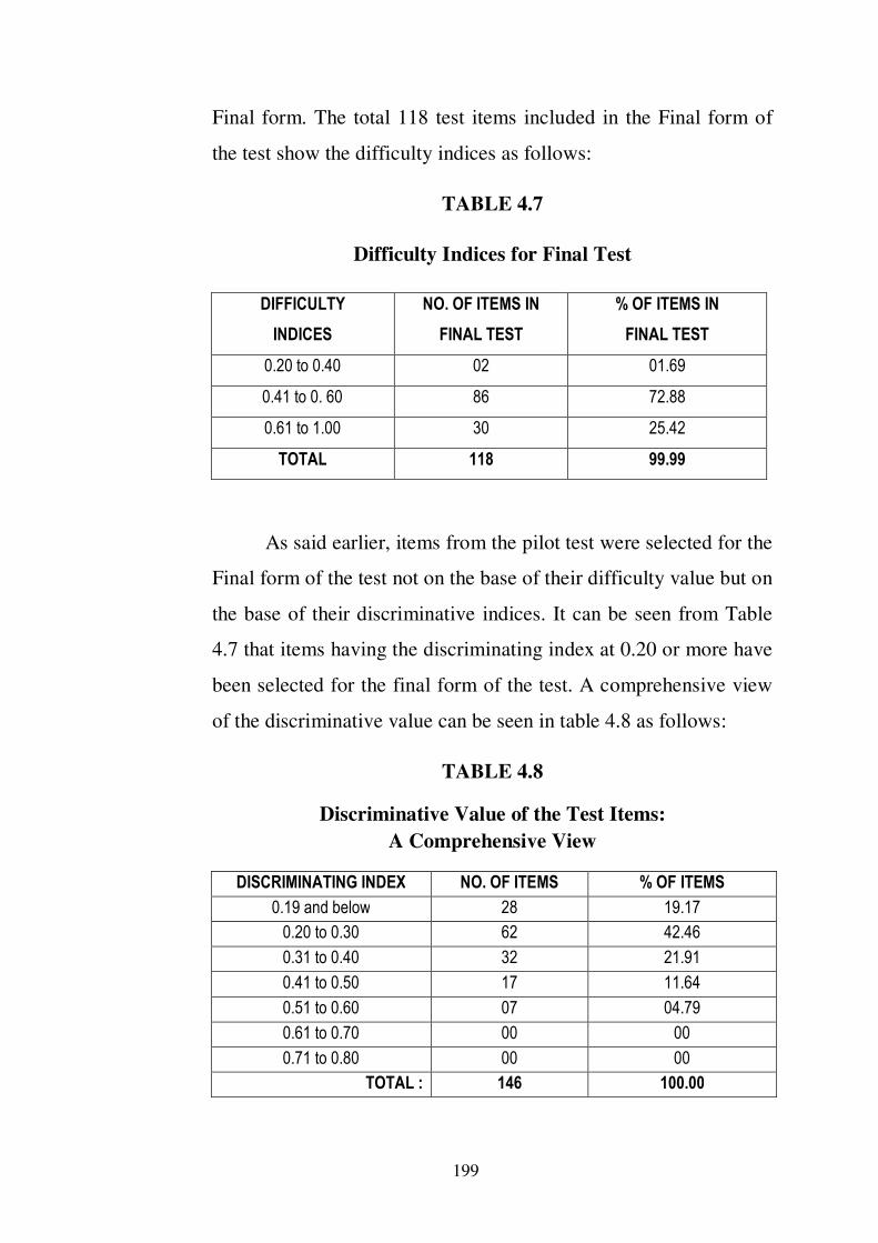
199

Final form. The total 118 test items included in the Final form of

the test show the difficulty indices as follows:

TABLE 4.7

Difficulty Indices for Final Test

DIFFICULTY

INDICES

NO. OF ITEMS IN

FINAL TEST

% OF ITEMS IN

FINAL TEST

0.20 to 0.40 02 01.69

0.41 to 0. 60 86 72.88

0.61 to 1.00 30 25.42

TOTAL 118 99.99

As said earlier, items from the pilot test were selected for the

Final form of the test not on the base of their difficulty value but on

the base of their discriminative indices. It can be seen from Table

4.7 that items having the discriminating index at 0.20 or more have

been selected for the final form of the test. A comprehensive view

of the discriminative value can be seen in table 4.8 as follows:

TABLE 4.8

Discriminative Value of the Test Items:

A Comprehensive View

DISCRIMINATING INDEX NO. OF ITEMS % OF ITEMS

0.19 and below 28 19.17

0.20 to 0.30 62 42.46

0.31 to 0.40 32 21.91

0.41 to 0.50 17 11.64

0.51 to 0.60 07 04.79

0.61 to 0.70 00 00

0.71 to 0.80 00 00

TOTAL : 146 100.00

200

It can be noted from table 4.8 that items having 0.19 or

below discriminative value were rejected for items inclusion in the

final test just as it was done for the Pre-Pilot Test. It can be seen

from Table 4.8 that out of the total 146 test items, of the pilot form,

as many as 28 i.e. 19 percentage items show 0.19 and below

discriminative value. Naturally, these items have been rejected in

the Final Form of the test. This means that there were 146 test

items in the Pilot Form of the test and out of them total 118 items

have been selected for the Final Form of the test. Hence, there is no

doubt about the careful construction of the pilot test.

It should be viewed also from the point of view of the sub-

tests. The whole test consisted of 5 sub-tests; the 5th

one is in 3

sections as it was in Pre-Pilot form. Table 4.9 shows the sub-test

wise total items and discriminative values.

TABLE 4.9

Sub-test wise Distribution of the Test Items Selected for the Pilot

Form on the basis of their Discriminative Power

SUB

TEST

NO. OF ITEMS

IN PRE-PILOT

TEST

ITEMS BELOW THE

DISCRIMINATIVE

VALUE 0.20

ITEMS RETAINED FOR

FINAL FORM

NO. OF

ITEMS

% OF

ITEMS

NO. OF

ITEMS

% OF

ITEMS

I 23 03 10.71 20 16.94

II 33 06 21.42 27 22.88

III 23 03 10.71 20 16.94

IV 22 04 14.28 18 15.25

V 45 12 42.85 33 27.96

TOTAL 146 28 19.17 118 80.82

201

Table 4.9 indicates that out of total 23, 33, 23, 22 and 45 test

items respectively in sub-tests I, II, III, IV, and V of Pilot test, only

20, 27, 20, 18 and 33 test items have been selected for the

subsequent Final Form of the Test.

4.2.3 Final Test :

This section is written on the discussion regarding the final form of

the test.

4.2.3.1 Construction of Final Test

Final test was constructed on the basis of analysis of the

results of the pilot form. This final form was also prepared in five

sub-tests.

As against 23, 33, 23, 22 and 45 test items making the total

146 respectively in sub-tests I, II, III, IV, and V of Pilot test, only

20, 27, 20, 18 and 33 (total 118) test items were selected

respectively in five sub-tests of the Final Form.

Table 4.10 shows distribution of test items in the final test

form from the point of view of their discriminative values.

TABLE 4.10

Distribution of Test Items of the Final Test as per

Discriminative Value

DISCRIMINATIVE VALUE

NO. OF TEST ITEMS

TOTAL SUB TESTS

I II III IV V

0.51 to 0.55 1 1 1 1 1 5

0.46 to 0.50 1 1 1 1 2 6

0.41 to 0.45 3 0 2 1 0 6

0.36 to 0.40 0 6 2 2 6 16

0.31 to 0.35 4 2 3 4 6 19

0.26 to 0.30 7 3 6 5 5 26

0.21 to 0.25 4 14 5 4 13 40

TOTAL 20 27 20 18 33 118

202

Table 4.10 shows that no test item in any sub-test has shown

discriminative value above 0.55. Only 1 item in each sub-test can

be seen in the range of 0.51 to 0.55. Similarly, only 1 test item can

be seen in the range of 0.46 to 0.50, except in sub-test- V, where 2

test items can be found. The the maximum number of test items can

be found in the range of 0.36 to 0.40, 0.31 to 0.35, and 0.26 to 0.30,

where there were 16, 19 and 26 items respectively in all five sub-

tests. The highest no. of items total 40 test items can be seen in the

lowest range – 0.21 to 0.25.

4.2.3.2 Final Test and Answer sheet

The researcher had predetermined to get the Final test

printed in press to make it more user-friendly, attractive and

legible. The size of the test booklet was selected referring different

sizes for test booklets. Finally, the matter of each five sub-tests was

handed over in a press with necessary instructions. It was decided

to attach with this five sub-tests, two more ready-made tests used

by the researcher – 1: Emotional Intelligence test by Dr. Pallavi

Patel and Hitesh Patel and 2: Adopted version of Gardner’s

Intelligence test. Total one thousand test booklets and answer

sheets were prepared for the final data collection. A copy of the

Final test booklet with answer key is put-up in Appendix – V for

its origin.

General instructions for respondents have been printed on

the cover page. Instructions along with illustrations for each sub-

test have been given in the beginning of the concerned sub-test.

The respondents had fill-up preliminary information at the top of

the answer sheet before they fill-up their answers on the answer

203

sheet. Each section of the test was paralleled with the answer sheet.

Each item was presented in serial order with number of all the

alternative responses. Order of distracters was also changed in

some of the test items and correct choices were placed at random

with a view to avoid any sequential order in answers. It was clear

that no change in wording was made in any item; only the

distracters were changed as per the need. The respondents had to

fill-up their correct choice by encircling the right option.

4.2.3.3 Sample for the Final Test

Analysis shows that the sample for final form of the test has

been drawn to make the same ‘a classified cluster sample’. A fairly

good number of 35 B. Ed colleges of Gujarat were consulted for

the final administration of the test in 2010-11. As a result of this

fairly a large number of 1000 respondents could be found with

correct responses from 17 B. Ed. Colleges throughout all the four

regions of Gujarat – South Gujarat, Middle Gujarat, Saurashtra and

North Gujarat. Six universities of the state have been taken as

different stratum and 17 colleges of these universities have been

considered as clusters. Total number of sample drawn on this basis

comes to 1000 B. Ed. Students of 325 male and 675 female ones,

as represented in details in Table 3.2 in the previous chapter – 3.

4.2.3.4 Administration of the Final Test

The researcher had administered the test personally at all

places with necessary rapport with respondents and with all

precautions. The final test was administered in the months of

204

December, January and February in the year 2010-11 with the prior

contacts and permission of the principals of the respective colleges.

4.2.3.5 Time Limit

Before giving a test to a large sample for establishing the

norms, it is essential to fix appropriate time limit for answering the

test. The time limit to be fixed largely depends upon the purpose of

the test. In case of power test, the time limit is fixed in such a way

as almost all individuals have opportunity to consider all the items

of the test.

In pilot test, about 40 to 50 seconds were required for one

item and total 120 minutes were calculated for the whole test. But

practical administration of the test took only 95 minutes. The time

limit is generally decided by considering the record of the time

taken by different individuals at the time of the pilot test. This can

give approximate time. In order to decide the exact time to be

allowed to answer the questions, some definite criteria have to be

fixed. There are different views about the time to be allowed to

answer the test. This becomes clear from the following statement

of Ross.9

“Lindquist suggests that in general achievement tests, the

time allowance should be so adjusted that 75 percent of the pupils

will have time at least to consider all items in each section. Ruth

seemed to favour time limits so that 90% can attempt all items

within their power.”

205

From this it was decided that the time allowance be fixed in

such a way that 75% of B. Ed. Students will have time at least to

consider all items. The time estimated in taking the entire final test

was computed to be 120 minutes. There were 118 test items in the

final form and that would take 80 minutes at the usual rate of half a

minute per item as experienced in pilot administration. Adding 05

minutes for distribution of the test booklet and answer sheets, 05

minutes to collect the test booklets and answer sheets and 10

minutes more for additional two tests, in all the total time required

would be 100 minutes. The respondents took 90 minutes on

average for responding to the whole test.

4.2.3.6 Scoring the Test

After administering the test, the next huge task was that of

scoring. The same scoring method, as was followed in the pilot

test. The same was followed here also. No change was necessary in

the scoring pattern. The scoring pattern, thus, is a standardised one

for scoring the present test.

No help was taken from any person for scoring. So there was

no question of any scoring errors being committed. The researcher

personally assessed all the 1000 answer sheets. It took almost 1

month to compute the score.

The the maximum score that a respondent can obtain on this

test is 118 and the the minimum score that can be obtained is

naturally zero. The highest score obtained on the test was 94 and

the lowest score was 38.5.

206

o SETTING-UP DIRECTIONS FOR ADMINISTRSTION AND

SCORING; THE ESTABLISHMENT OF NORMS

4.3 Establishment of Norms

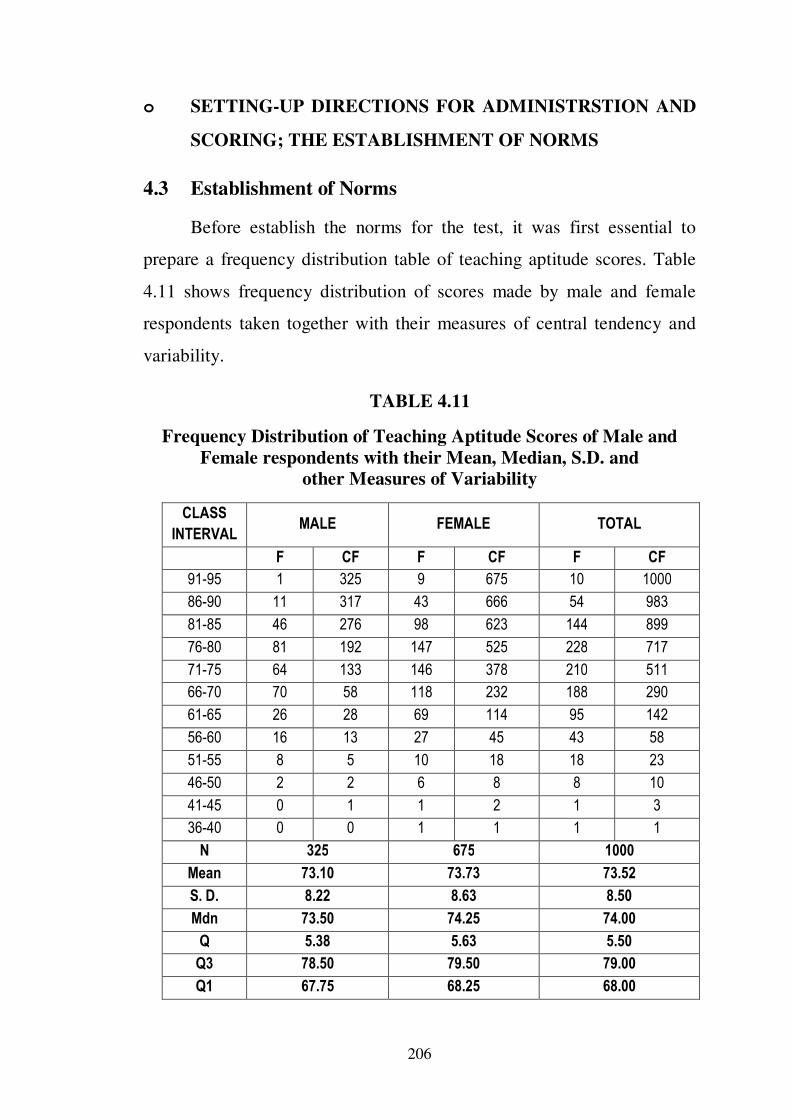
Before establish the norms for the test, it was first essential to

prepare a frequency distribution table of teaching aptitude scores. Table

4.11 shows frequency distribution of scores made by male and female

respondents taken together with their measures of central tendency and

variability.

TABLE 4.11

Frequency Distribution of Teaching Aptitude Scores of Male and

Female respondents with their Mean, Median, S.D. and

other Measures of Variability

CLASS

INTERVAL MALE FEMALE TOTAL

F CF F CF F CF

91-95 1 325 9 675 10 1000

86-90 11 317 43 666 54 983

81-85 46 276 98 623 144 899

76-80 81 192 147 525 228 717

71-75 64 133 146 378 210 511

66-70 70 58 118 232 188 290

61-65 26 28 69 114 95 142

56-60 16 13 27 45 43 58

51-55 8 5 10 18 18 23

46-50 2 2 6 8 8 10

41-45 0 1 1 2 1 3

36-40 0 0 1 1 1 1

N 325 675 1000

Mean 73.10 73.73 73.52

S. D. 8.22 8.63 8.50

Mdn 73.50 74.25 74.00

Q 5.38 5.63 5.50

Q3 78.50 79.50 79.00

Q1 67.75 68.25 68.00

207

From table 4.11, it indicates that there is difference in the mean

performances of male and female candidates. Therefore, before

establishing sex norms, percentile and standard score, it was thought to

test the significance of mean differences. T-test technique was used for

this. The summary of t-ratio is put up in table 4.12 as follows;

4.3.1 Difference between the Mean Teaching Aptitude Scores of

Male and Female B.Ed. Students:

The t-values were calculated to check the objective no. 8 and the

null hypothesis no. 12 of this study. The values are tabulated in Table

4.12.

Table 4.12

The Mean, SD and t-values of Teaching Aptitude

Scores of Male and Female

Statistics →

Sample ↓

N Mean SD Mean

Difference

t -

value

Sig.

level

Male 325 73.10 8.22

0.63 1.13* N.S.

Female 675 73.73 8.63

* Not Significant at 0.05 level

It is observed from the table 4.12 that mean difference in

performance between male and female B. Ed. Students comes to be 0.63

and the t-value is 1.13. The Table values should be t0.05 = 1.96 and t0.01 =

2.58 with df = 1000 as per Table C. Whereas, the present t-value is 1.13,

which does not exceeds the table value of ‘t’ at 0.05 level of the

significance. Hence, the mean difference between the two groups is not

significant. Consequently, the hypothesis “H12 : There is no significant

208

difference between the mean Teaching Aptitude Score of Male and

Female B.Ed. Students” is accepted. That means the mean significant

difference between the teaching aptitude score of male and female B.Ed.

students is accidental and not the real one. Hence, the mean teaching

aptitude scores of male and female students are assumed to be

homogenous.

The Mean teaching aptitude scores of male and female are

presented in the Graph 4.1

Graph 4.1

The Mean Teaching Aptitude Scores of Male and Female

From graph – 4.1 it can be clearly seen that there is a little (not

Significant) difference in mean teaching aptitude scores of male and

female B.Ed. students. The difference is accidental and not the real one.

Hence, it can be said that there is no gender difference in teaching

aptitude scores.

Therefore, the investigator has not presented the “Sex Norms” of

B.Ed. students, as they are assumed to be homogenous.

209

Ordinarily, frequency distribution conveys a picture of a situation

only in numbers. However, for quick and easy grasp, a pictorial

presentation would not be out of place. Pictorial presentation of frequency

distribution is shown by graphs. This pictorial presentation is also useful

in comparing the results with the normal curve. The frequency curve of

the whole sample is presented in the following graph 4.2

GRAPH : 4.2

HISTOGRAM, FREQUENCY CURVE

FOR WHOLE SAMPLE (N = 1000)

Graph : 4.2 shows histogram and frequency polygon on the same

axis of a whole sample of 1000 respondents. The data have been shown in

Table 4.11. Graph – 4.2 shows that frequency polygon is skewed than

smoothed frequency polygon. Distribution towards both the ends is

normal. At the mean point, the highest of the frequency polygon is more

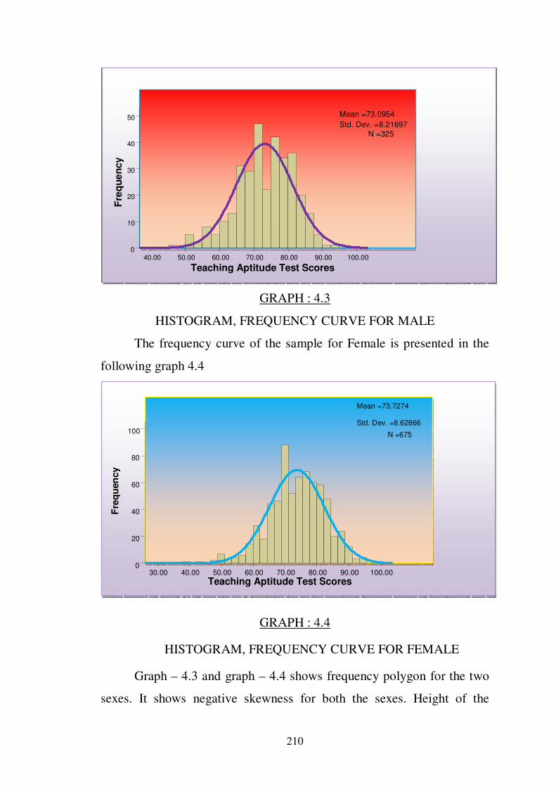
than the smoothed one. The frequency curve of the sample for Male is

presented in the following graph 4.3

100.0090.0080.0070.0060.0050.0040.0030.00

Teaching Aptitude Test Scores

100

80

60

40

20

0

Mean =73.522

Std. Dev. =8.4981

N =1,000

Fre

qu

en

cy

210

GRAPH : 4.3

HISTOGRAM, FREQUENCY CURVE FOR MALE

The frequency curve of the sample for Female is presented in the

following graph 4.4

GRAPH : 4.4

HISTOGRAM, FREQUENCY CURVE FOR FEMALE

Graph – 4.3 and graph – 4.4 shows frequency polygon for the two

sexes. It shows negative skewness for both the sexes. Height of the

100.0090.0080.00 70.00 60.00 50.00 40.00

Teaching Aptitude Test Scores

50

40

30

20

10

0

Fre

qu

en

cy

Mean =73.0954 Std. Dev. =8.21697

N =325

100.00 90.0080.0070.0060.0050.00 40.00 30.00 Teaching Aptitude Test Scores

100

80

60

40

20

0

Fre

qu

en

cy

Mean =73.7274

Std. Dev. =8.62866 N =675

211

frequency polygon for female is higher than that of the male group. The

frequency polygon of the female is more Kurtic than that of the male.

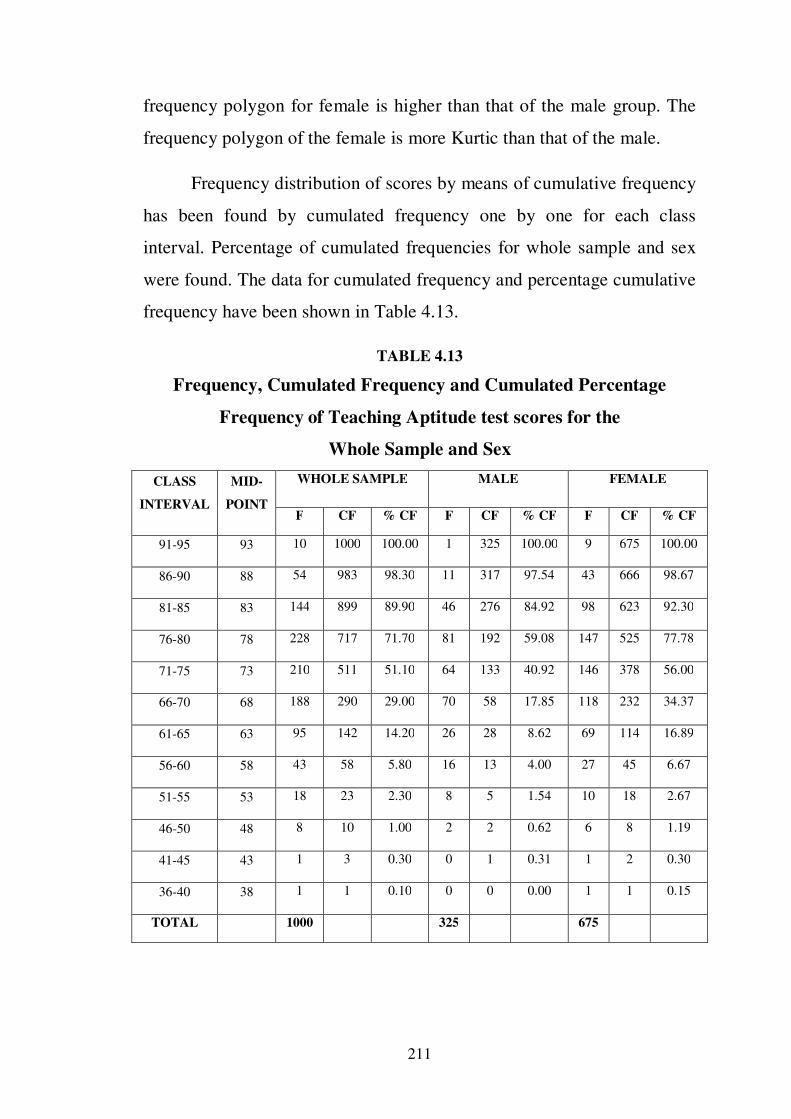
Frequency distribution of scores by means of cumulative frequency

has been found by cumulated frequency one by one for each class

interval. Percentage of cumulated frequencies for whole sample and sex

were found. The data for cumulated frequency and percentage cumulative

frequency have been shown in Table 4.13.

TABLE 4.13

Frequency, Cumulated Frequency and Cumulated Percentage

Frequency of Teaching Aptitude test scores for the

Whole Sample and Sex

CLASS

INTERVAL

MID-

POINT

WHOLE SAMPLE MALE FEMALE

F CF % CF F CF % CF F CF % CF

91-95 93 10 1000 100.00 1 325 100.00 9 675 100.00

86-90 88 54 983 98.30 11 317 97.54 43 666 98.67

81-85 83 144 899 89.90 46 276 84.92 98 623 92.30

76-80 78 228 717 71.70 81 192 59.08 147 525 77.78

71-75 73 210 511 51.10 64 133 40.92 146 378 56.00

66-70 68 188 290 29.00 70 58 17.85 118 232 34.37

61-65 63 95 142 14.20 26 28 8.62 69 114 16.89

56-60 58 43 58 5.80 16 13 4.00 27 45 6.67

51-55 53 18 23 2.30 8 5 1.54 10 18 2.67

46-50 48 8 10 1.00 2 2 0.62 6 8 1.19

41-45 43 1 3 0.30 0 1 0.31 1 2 0.30

36-40 38 1 1 0.10 0 0 0.00 1 1 0.15

TOTAL 1000 325 675

212

From above table 4.13 the differences in cumulated percentage

frequencies between the two sexes can be seen. This was used in further

calculation of establishment of norms.

The cumulative percentage curve has been shown in Graph 4.5 as

follows :

GRAPH : 4.5

CUMULATIVE FREQUENCY GRAPH FOR WHOLE SAMPLE OF

TEACHING APTITUDE TEST

Graph – 4.5 shows the cumulative frequency curve for the whole

sample of the teaching aptitude scores. This is ‘S’ shaped curve.

Frequency, Cumulated Frequency and Cumulated Percentage frequency

of teaching aptitude scores for the whole sample and sexes have been

shown in Table 4.13.

213

A cumulative percentage curve has also been drawn for different

sexes by using the data given in Table 4.13 and presented in the graph 4.5

as follows :

GRAPH : 4.6

CUMULATIVE FREQUENCY GRAPH FOR SEXES OF

TEACHING APTITUDE TEST

Graph – 4.6 shows the cumulative frequency curve for different

sexes i.e. male and female respectively. This is also ‘S’ shaped curve.

Frequency, Cumulated Frequency and Cumulated Percentage frequency

of teaching aptitude scores for the whole sample and sexes have been

shown in Table 4.13.

From frequency smoothed frequency was calculated and presented

in the table 4.14 as follows :

214

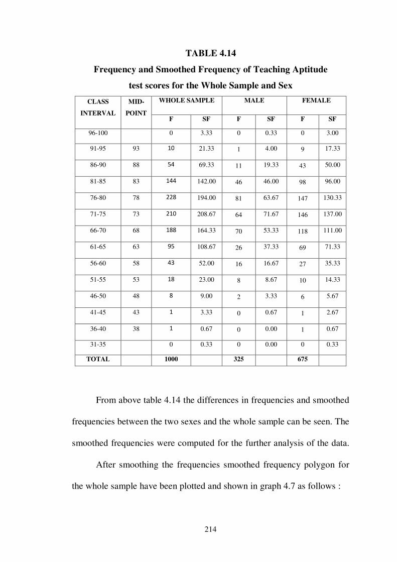
TABLE 4.14

Frequency and Smoothed Frequency of Teaching Aptitude

test scores for the Whole Sample and Sex

CLASS

INTERVAL

MID-

POINT

WHOLE SAMPLE MALE FEMALE

F SF F SF F SF

96-100 0 3.33 0 0.33 0 3.00

91-95 93 10 21.33 1 4.00 9 17.33

86-90 88 54 69.33 11 19.33 43 50.00

81-85 83 144 142.00 46 46.00 98 96.00

76-80 78 228 194.00 81 63.67 147 130.33

71-75 73 210 208.67 64 71.67 146 137.00

66-70 68 188 164.33 70 53.33 118 111.00

61-65 63 95 108.67 26 37.33 69 71.33

56-60 58 43 52.00 16 16.67 27 35.33

51-55 53 18 23.00 8 8.67 10 14.33

46-50 48 8 9.00 2 3.33 6 5.67

41-45 43 1 3.33 0 0.67 1 2.67

36-40 38 1 0.67 0 0.00 1 0.67

31-35 0 0.33 0 0.00 0 0.33

TOTAL 1000 325 675

From above table 4.14 the differences in frequencies and smoothed

frequencies between the two sexes and the whole sample can be seen. The

smoothed frequencies were computed for the further analysis of the data.

After smoothing the frequencies smoothed frequency polygon for

the whole sample have been plotted and shown in graph 4.7 as follows :

215

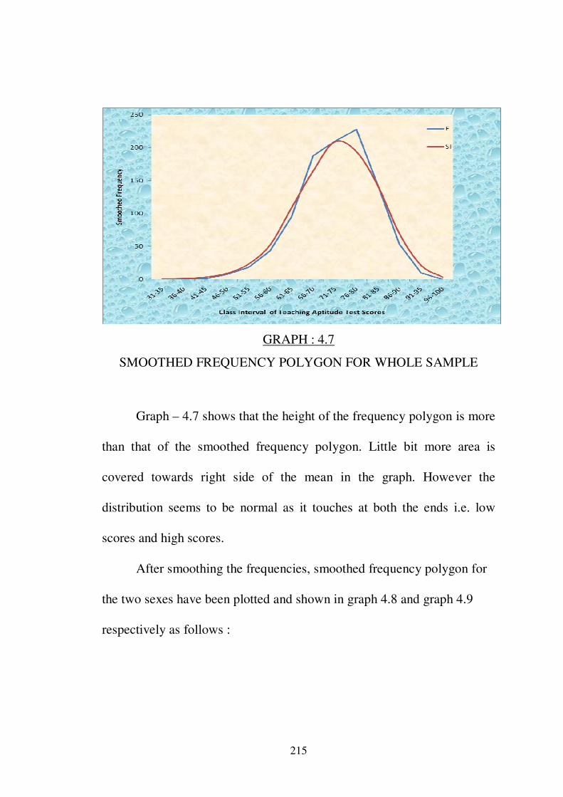
GRAPH : 4.7

SMOOTHED FREQUENCY POLYGON FOR WHOLE SAMPLE

Graph – 4.7 shows that the height of the frequency polygon is more

than that of the smoothed frequency polygon. Little bit more area is

covered towards right side of the mean in the graph. However the

distribution seems to be normal as it touches at both the ends i.e. low

scores and high scores.

After smoothing the frequencies, smoothed frequency polygon for

the two sexes have been plotted and shown in graph 4.8 and graph 4.9

respectively as follows :

216

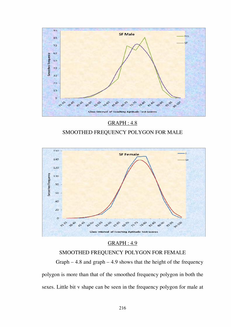
GRAPH : 4.8

SMOOTHED FREQUENCY POLYGON FOR MALE

GRAPH : 4.9

SMOOTHED FREQUENCY POLYGON FOR FEMALE

Graph – 4.8 and graph – 4.9 shows that the height of the frequency

polygon is more than that of the smoothed frequency polygon in both the

sexes. Little bit v shape can be seen in the frequency polygon for male at

217

the mean level, but after smoothing the shape was turned normal.

However, the distribution on both the sexes seems to be normal as it

touches at both the ends i.e. low scores and high scores.

In order to decide the nature of the distribution of test scores, it was

essential to find out Percentile norms of teaching aptitude scores.

The percentile norms are given in table 4.15.

Percentile ranks were computed by using the following formula10

;

PP

Where,

PP = Percentage of the distribution wanted,

l = exact lower limit of the class interval upon which PP lies,

PN = part of N to be counted off in order to reach PP ,

F = Sum of all scores upon intervals below l,

Fp = number of scores within the interval upon which PP falls,

i = length of the class interval.

218

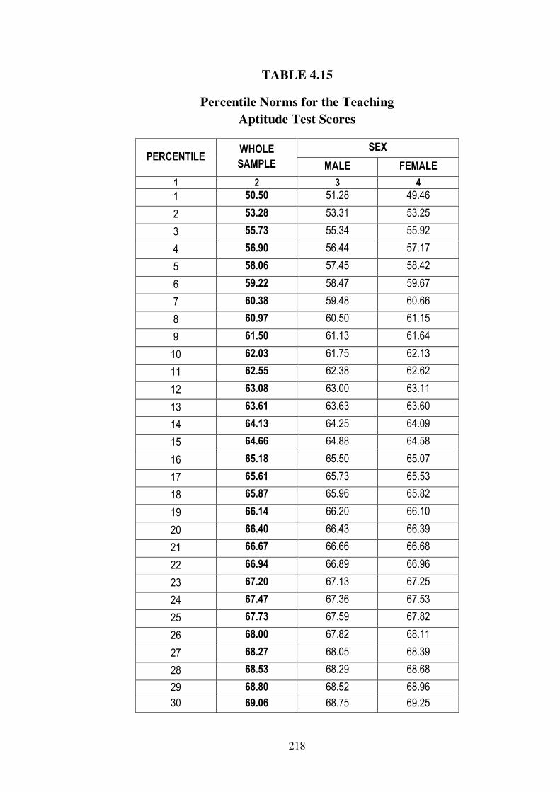
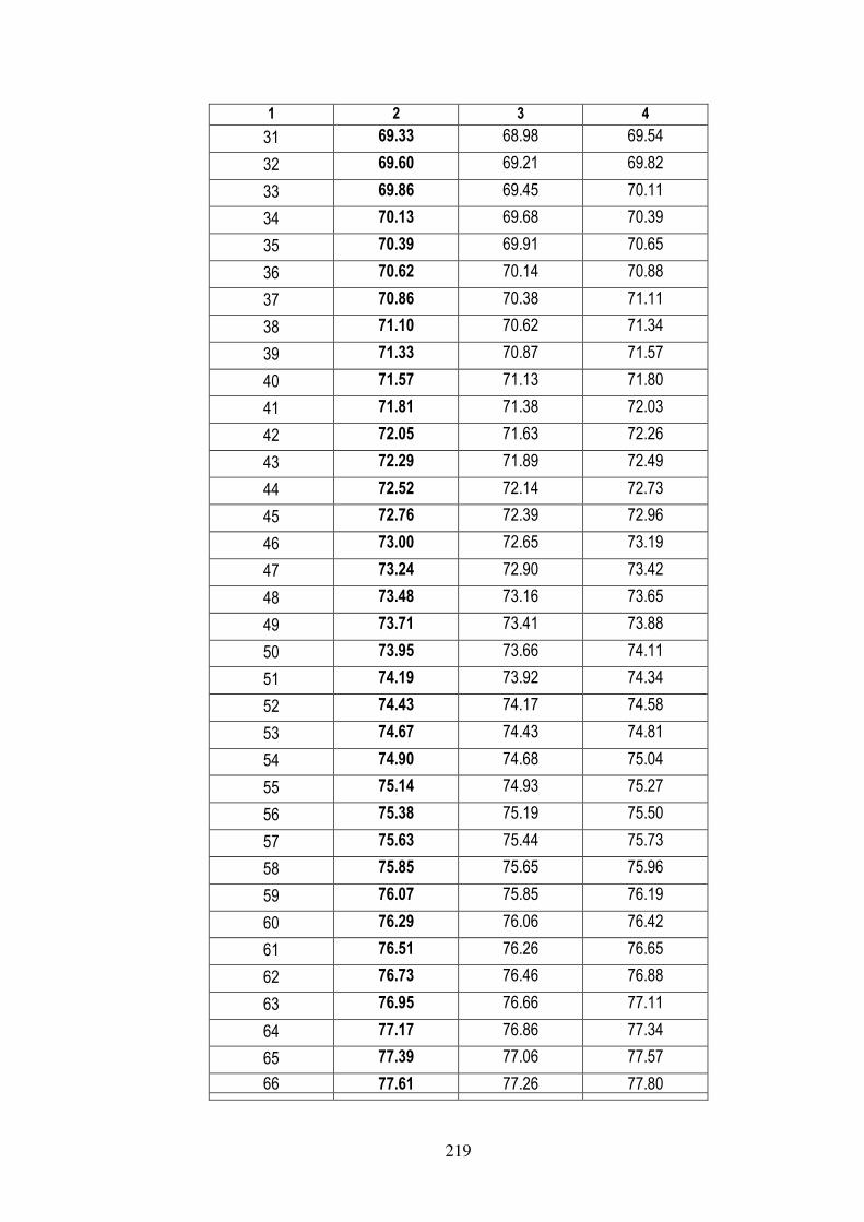
TABLE 4.15

Percentile Norms for the Teaching

Aptitude Test Scores

PERCENTILE WHOLE

SAMPLE

SEX

MALE FEMALE

1 2 3 4

1 50.50 51.28 49.46

2 53.28 53.31 53.25

3 55.73 55.34 55.92

4 56.90 56.44 57.17

5 58.06 57.45 58.42

6 59.22 58.47 59.67

7 60.38 59.48 60.66

8 60.97 60.50 61.15

9 61.50 61.13 61.64

10 62.03 61.75 62.13

11 62.55 62.38 62.62

12 63.08 63.00 63.11

13 63.61 63.63 63.60

14 64.13 64.25 64.09

15 64.66 64.88 64.58

16 65.18 65.50 65.07

17 65.61 65.73 65.53

18 65.87 65.96 65.82

19 66.14 66.20 66.10

20 66.40 66.43 66.39

21 66.67 66.66 66.68

22 66.94 66.89 66.96

23 67.20 67.13 67.25

24 67.47 67.36 67.53

25 67.73 67.59 67.82

26 68.00 67.82 68.11

27 68.27 68.05 68.39

28 68.53 68.29 68.68

29 68.80 68.52 68.96

30 69.06 68.75 69.25

219

1 2 3 4

31 69.33 68.98 69.54

32 69.60 69.21 69.82

33 69.86 69.45 70.11

34 70.13 69.68 70.39

35 70.39 69.91 70.65

36 70.62 70.14 70.88

37 70.86 70.38 71.11

38 71.10 70.62 71.34

39 71.33 70.87 71.57

40 71.57 71.13 71.80

41 71.81 71.38 72.03

42 72.05 71.63 72.26

43 72.29 71.89 72.49

44 72.52 72.14 72.73

45 72.76 72.39 72.96

46 73.00 72.65 73.19

47 73.24 72.90 73.42

48 73.48 73.16 73.65

49 73.71 73.41 73.88

50 73.95 73.66 74.11

51 74.19 73.92 74.34

52 74.43 74.17 74.58

53 74.67 74.43 74.81

54 74.90 74.68 75.04

55 75.14 74.93 75.27

56 75.38 75.19 75.50

57 75.63 75.44 75.73

58 75.85 75.65 75.96

59 76.07 75.85 76.19

60 76.29 76.06 76.42

61 76.51 76.26 76.65

62 76.73 76.46 76.88

63 76.95 76.66 77.11

64 77.17 76.86 77.34

65 77.39 77.06 77.57

66 77.61 77.26 77.80

220

1 2 3 4

67 77.82 77.46 78.03

68 78.04 77.66 78.26

69 78.26 77.86 78.48

70 78.48 78.06 78.71

71 78.70 78.26 78.94

72 78.92 78.46 79.17

73 79.14 78.66 79.40

74 79.36 78.86 79.63

75 79.58 79.06 79.86

76 79.80 79.27 80.09

77 80.02 79.47 80.32

78 80.24 79.67 80.58

79 80.46 79.87 80.92

80 80.78 80.07 81.27

81 81.13 80.27 81.61

82 81.47 80.47 81.95

83 81.82 80.80 82.30

84 82.17 81.15 82.64

85 82.51 81.51 82.99

86 82.86 81.86 83.33

87 83.21 82.21 83.68

88 83.56 82.57 84.02

89 83.90 82.92 84.36

90 84.25 83.27 84.71

91 84.60 83.63 85.05

92 84.94 83.98 85.40

93 85.29 84.33 86.05

94 85.87 84.68 86.84

95 86.80 85.04 87.62

96 87.72 85.39 88.41

97 88.65 86.52 89.19

98 89.57 88.00 89.98

99 90.50 89.48 91.75

100 95.50 95.50 95.50

221

4.3.2 Deciding the Nature of the Distribution of Test Scores

If the test scores are distributed normally, we can assume that the

tool is satisfactory.

The following two procedures were used to study the distribution

of the aptitude test scores.

o Calculation of ‘Skewness’ and

o Calculation of ‘Kurtosis’.

o Calculation of Skewness of the distribution :

There are two different formulas for the calculation of

skewness. Skewness is calculated using both these formulas. The

formulae are as follows:11

(i) SK = … (A)

(ii) SK = … (B)

o Calculation of SK by formula ‘A’ :

Mean = 73.52

Median = 74.00 * from Table 4.11

SD = 8.50

∴ SK =

=

= -0.169

222

The value of skewness obtained indicated a little negative

skewness.

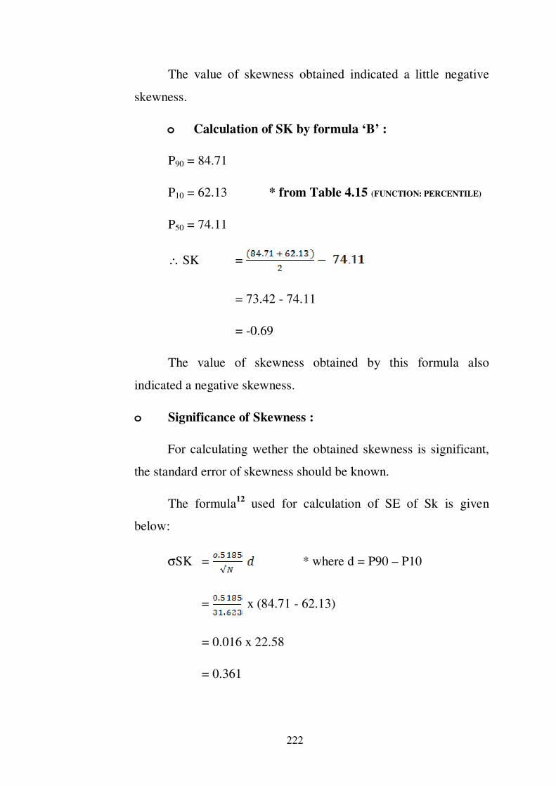
o Calculation of SK by formula ‘B’ :

P90 = 84.71

P10 = 62.13 * from Table 4.15 (FUNCTION: PERCENTILE)

P50 = 74.11

∴ SK =

= 73.42 - 74.11

= -0.69

The value of skewness obtained by this formula also

indicated a negative skewness.

o Significance of Skewness :

For calculating wether the obtained skewness is significant,

the standard error of skewness should be known.

The formula12

used for calculation of SE of Sk is given

below:

σSK = * where d = P90 – P10

= x (84.71 - 62.13)

= 0.016 x 22.58

= 0.361

223

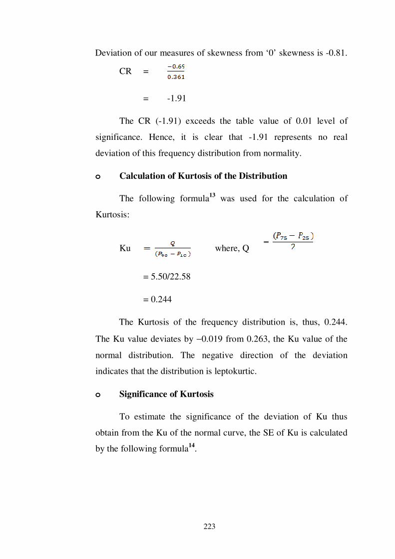
Deviation of our measures of skewness from ‘0’ skewness is -0.81.

CR =

= -1.91

The CR (-1.91) exceeds the table value of 0.01 level of

significance. Hence, it is clear that -1.91 represents no real

deviation of this frequency distribution from normality.

o Calculation of Kurtosis of the Distribution

The following formula13

was used for the calculation of

Kurtosis:

Ku where, Q

= 5.50/22.58

= 0.244

The Kurtosis of the frequency distribution is, thus, 0.244.

The Ku value deviates by −0.019 from 0.263, the Ku value of the

normal distribution. The negative direction of the deviation

indicates that the distribution is leptokurtic.

o Significance of Kurtosis

To estimate the significance of the deviation of Ku thus

obtain from the Ku of the normal curve, the SE of Ku is calculated

by the following formula14

.

224

σKu

=0.009

And the CR here D=deviation of Ku of

the obtained distribution

= -2.11 from Ku (0.263) of normal

distribution.

The CR (-2.11) does not falls within the ± 1.96 limits which

determine the 0.05 level of significance.

Hence, it is clear that 0.244 represents no real deviation of

this frequency distribution from normality.

4.3.1 Standard Score and T score

In teaching aptitude test, generally percentile norms,

standard scores and T-score norms are established. Therefore, for

the present test percentile norms, standard scores and T scores also

have been established and reported in this chapter.

The percentile norms for male and female are presented in

Table 4.15.

(A) Standard Score Norms

The raw scores obtained on the test were converted into the

standard scores with the help of the following formula10. The shift

from raw to standard score requires a linear transformation. This

225

transformation does not change the shape of the distribution in any

way.

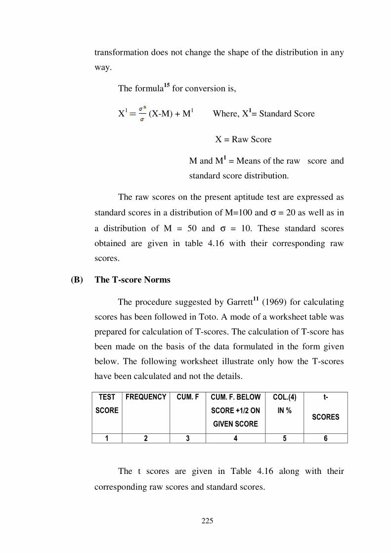
The formula15

for conversion is,

X1

(X-M) + M1 Where, X

1= Standard Score

X = Raw Score

M and M1 = Means of the raw score and

standard score distribution.

The raw scores on the present aptitude test are expressed as

standard scores in a distribution of M=100 and σ = 20 as well as in

a distribution of M = 50 and σ = 10. These standard scores

obtained are given in table 4.16 with their corresponding raw

scores.

(B) The T-score Norms

The procedure suggested by Garrett11

(1969) for calculating

scores has been followed in Toto. A mode of a worksheet table was

prepared for calculation of T-scores. The calculation of T-score has

been made on the basis of the data formulated in the form given

below. The following worksheet illustrate only how the T-scores

have been calculated and not the details.

TEST

SCORE

FREQUENCY CUM. F CUM. F. BELOW

SCORE +1/2 ON

GIVEN SCORE

COL.(4)

IN %

t-

SCORES

1 2 3 4 5 6

The t scores are given in Table 4.16 along with their

corresponding raw scores and standard scores.

226

TABLE 4.16

Raw Scores and their Corresponding

Standard Scores and t Scores

RAW SCORES STANDARD

SCORES M=100

SD=20

STANDARD

SCORES M=50

SD=10

t – SCORES

1 2 3 4

1 -81 -41 -

2 -79 -39 -

3 -76 -38 -

4 -74 -37 -

5 -71 -36 -

6 -69 -34 -

7 -66 -33 -

8 -64 -32 -

9 -61 -31 -

10 -59 -29 -

11 -56 -28 -

12 -54 -27 -

13 -51 -26 -

14 -49 -24 -

15 -46 -23 -

16 -44 -22 -

17 -41 -21 -

18 -39 -19 -

19 -36 -18 -

20 -34 -17 -

21 -31 -16 -

22 -29 -14 -

23 -26 -13 -

24 -24 -12 -

25 -21 -11 -

26 -19 -9 -

27 -16 -8 -

28 -14 -7 -

29 -11 -6 -

30 -9 -4 -

31 -6 -3 -

32 -4 -2 -

33 -1 -1 -

34 1 1 -

35 4 2 -

36 6 3 -

227

1 2 3 4

37 9 4 -

38 11 6 -

39 14 7 12

40 16 8 19

41 19 9 19

42 21 11 19

43 24 12 21

44 26 13 22

45 29 14 22

46 31 16 22

47 34 17 23

48 36 18 24

49 39 19 25

50 41 21 27

51 44 22 28

52 46 23 29

53 49 24 30

54 51 26 30

55 54 27 31

56 56 28 32

57 59 29 33

58 61 31 34

59 64 32 35

60 66 33 36

61 69 34 36

62 71 36 37

63 74 37 38

64 76 38 39

65 79 39 40

66 81 41 41

67 84 42 42

68 86 43 43

69 89 44 45

70 91 46 46

71 94 47 47

72 96 48 48

73 99 49 49

74 101 51 50

75 104 52 51

76 106 53 52

77 109 54 53

78 111 56 55

79 114 57 56

228

1 2 3 4

80 116 58 57

81 119 59 58

82 121 61 60

83 124 62 61

84 126 63 62

85 129 64 64

86 131 66 65

87 134 67 67

88 136 68 68

89 139 69 70

90 141 71 72

91 144 72 73

92 146 73 74

93 149 74 75

94 151 76 78

95 154 77 -

96 156 78 -

97 159 79 -

98 161 81 -

99 164 82 -

100 166 83 -

101 169 84 -

102 171 86 -

103 174 87 -

104 176 88 -

105 179 89 -

106 181 91 -

107 184 92 -

108 186 93 -

109 189 94 -

110 191 96 -

111 194 97 -

112 196 98 -

113 199 99 -

114 201 101 -

115 204 102 -

116 206 103 -

117 209 104 -

118 211 106 -

229

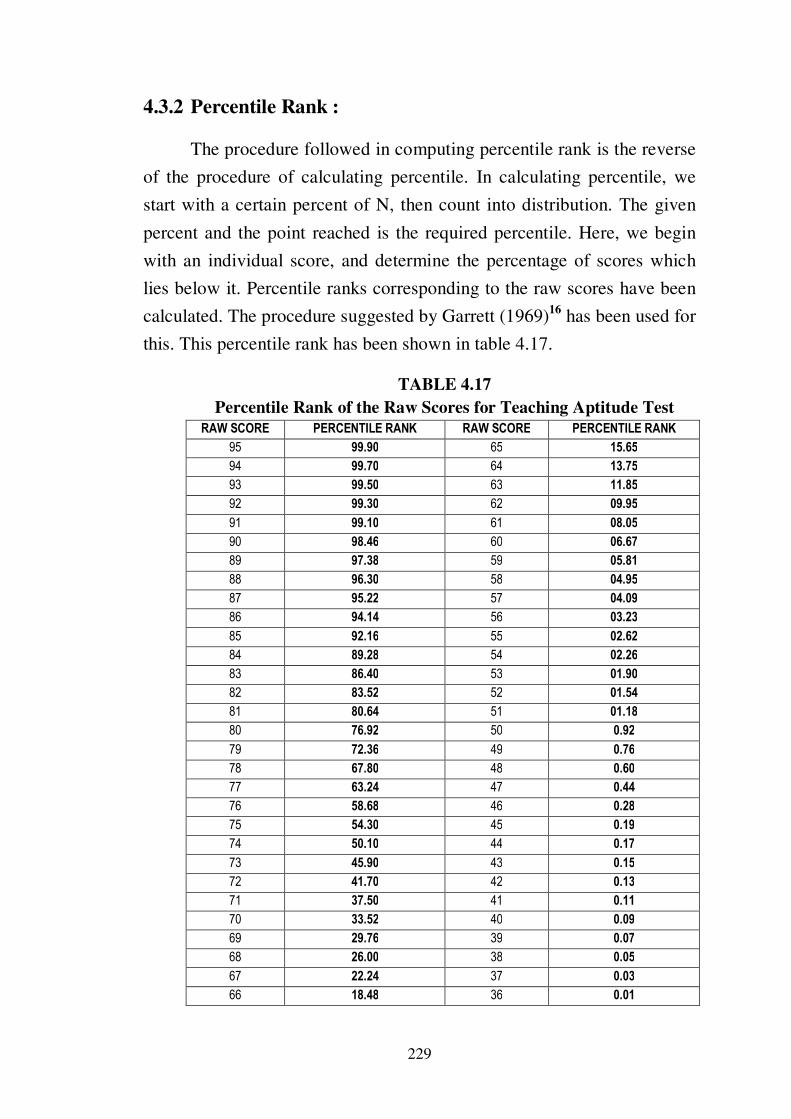
4.3.2 Percentile Rank :

The procedure followed in computing percentile rank is the reverse

of the procedure of calculating percentile. In calculating percentile, we

start with a certain percent of N, then count into distribution. The given

percent and the point reached is the required percentile. Here, we begin

with an individual score, and determine the percentage of scores which

lies below it. Percentile ranks corresponding to the raw scores have been

calculated. The procedure suggested by Garrett (1969)16

has been used for

this. This percentile rank has been shown in table 4.17.

TABLE 4.17

Percentile Rank of the Raw Scores for Teaching Aptitude Test

RAW SCORE PERCENTILE RANK RAW SCORE PERCENTILE RANK

95 99.90 65 15.65

94 99.70 64 13.75

93 99.50 63 11.85

92 99.30 62 09.95

91 99.10 61 08.05

90 98.46 60 06.67

89 97.38 59 05.81

88 96.30 58 04.95

87 95.22 57 04.09

86 94.14 56 03.23

85 92.16 55 02.62

84 89.28 54 02.26

83 86.40 53 01.90

82 83.52 52 01.54

81 80.64 51 01.18

80 76.92 50 0.92

79 72.36 49 0.76

78 67.80 48 0.60

77 63.24 47 0.44

76 58.68 46 0.28

75 54.30 45 0.19

74 50.10 44 0.17

73 45.90 43 0.15

72 41.70 42 0.13

71 37.50 41 0.11

70 33.52 40 0.09

69 29.76 39 0.07

68 26.00 38 0.05

67 22.24 37 0.03

66 18.48 36 0.01

230

o FOLLO-UP STUDIES TO DETERMINE THE PREDICTIVE

VALUE OF THE TEST BATTERY IN SELECTION AND IN

VOCATIONAL GUIDANCE

4.4 Reliability of the Test :

4.4.1 The Concept of Reliability :

No matter how carefully the test has been planned and

prepared, its merits should be established. Reliability and validity

are the essential qualities of a good test. It is, therefore, necessary

as a final check to study reliability and validity of the test.

According to Anastasi, any measuring device whatsoever must

fulfil conditions like reliability and validity if it is to be of any

service. In assessing value of a test, one should consider its

validity, reliability and usability. After estimating the norms on the

basis of the final results, it is essential for the test constructor to

obtain final evidence of reliability and validity of the test, to

establish its merits.

The concept of reliability has been defined by several in the

field. They are given below :

According to Robert Lado17

,

“If the scores of the students are stable the test is reliable,

if the scores tend to fluctuate for no apparent reason the test is

unreliable.”

Mehrens18

says,

“Reliability can be defined as the degree of consistency

between two measures of the same thing.”

231

Anastasi19

states,

“Reliability refers to the consistency of scores obtained

by the same individuals when re-examined with the same test

on different occasions,”

According to Freeman20

,

“Scores for the same individuals obtained on repeated

testing are not completely stable. Not only are there to be some

different chance determinants in operation at different time,

but it is quite normal for a human being to vary in

performance, generally within fairly narrow limit, from one

occasion to another.”

4.4.2 Methods of Establishing Reliability :

Reliability is purely a statistical concept. For establishing

reliability of the present test, the following methods have been

followed;

o Test-Retest method

o Split-half Method

o Kuder and Richardson Method

4.4.2.1 Test-Retest Method :

This Method involves,

o Obtaining repeated measures for the same individuals of

the same ability who are given the same test twice.

o Computation of correlations between the first and the

second set of scores.

232

The correlation co-efficient thus obtained indicates the

extent or magnitude of the certain factors like practice, confidence,

growth, physical facilities which play certain role on those two

different occasions of the test administration. To counteract the

effects of these variables, a fairly large sample would be needed.

Besides, the time interval should be adequate.

For the present study, reliability sample selected to apply

this method consisted of 100 B.Ed. students. They were retested

after an interval of about 5 to 6 months from the date of the first

test. The scores obtained on two different administrations of the

same test were used as two sets of scores for finding out the

correlation co-efficient. The correlation co-efficient was computed

by Pearson’s Product Moment method. On the basis of the data

furnished in the scatter diagram in Table 4.18.

TABLE 4.18

The Scatter Diagram of Scores obtained by the B.Ed. students for

Teaching Aptitude Test on two Successive

Administrations of the Test

S E C O N D A D M I N I S T R A T I O N

Class 36-

40

41-

45

46-

50

51-

55

56-

60

61-

65

66-

70

71-

75

76-

80

81-

85

86-

90

91-

95 FY

FI

RS

T

AD

MI

NI

ST

RA

TI

ON

91-95 1 1 2

86-90 1 4 5

81-85 3 4 10 17

76-80 5 5 9 19

71-75 1 2 3 19 25

66-70 1 1 5 5 5 17

61-65 1 2 3 5 11

56-60 2 2

51-55 1 1

46-50 0

41-45 1 1

36-40 0

FX 0 0 1 0 3 6 10 16 38 20 5 1 100

233

r = 0.7717 Test – test Reliability ‘r’ = 0.77

SEmean = 7.6733

SEr = 0.0407

4.4.2.2 Split-half Method :

This is the most widely used method of establishing the

reliability of the test because parallel from method as well as test-

retest method have certain limitations. To overcome the limitations

of these methods, the split-half method21

is used popularly.

This method involves splitting the whole test into two

reasonably equivalent halves. For making two equivalent halves,

usually pulling the odd numbered items for the other set of scores

is done. This method is preferred because it reasonably controls

such factors as practice, fatigue, distraction and mental set.

For this purpose, a sample of 100 B.Ed. students out of the

total sample of 1000 respondents was selected for applying ‘split-

half’ method to estimate reliability of the whole test. The scores

made by B.Ed. students on odd numbered and even numbered

items found out and were spited into two parts. The correlation

between the scores on odd and even numbered items was then

computed by using Pearson’s Product Moment method.

Table 4.19 shows the scatter diagram and split-half test

reliability of the test.

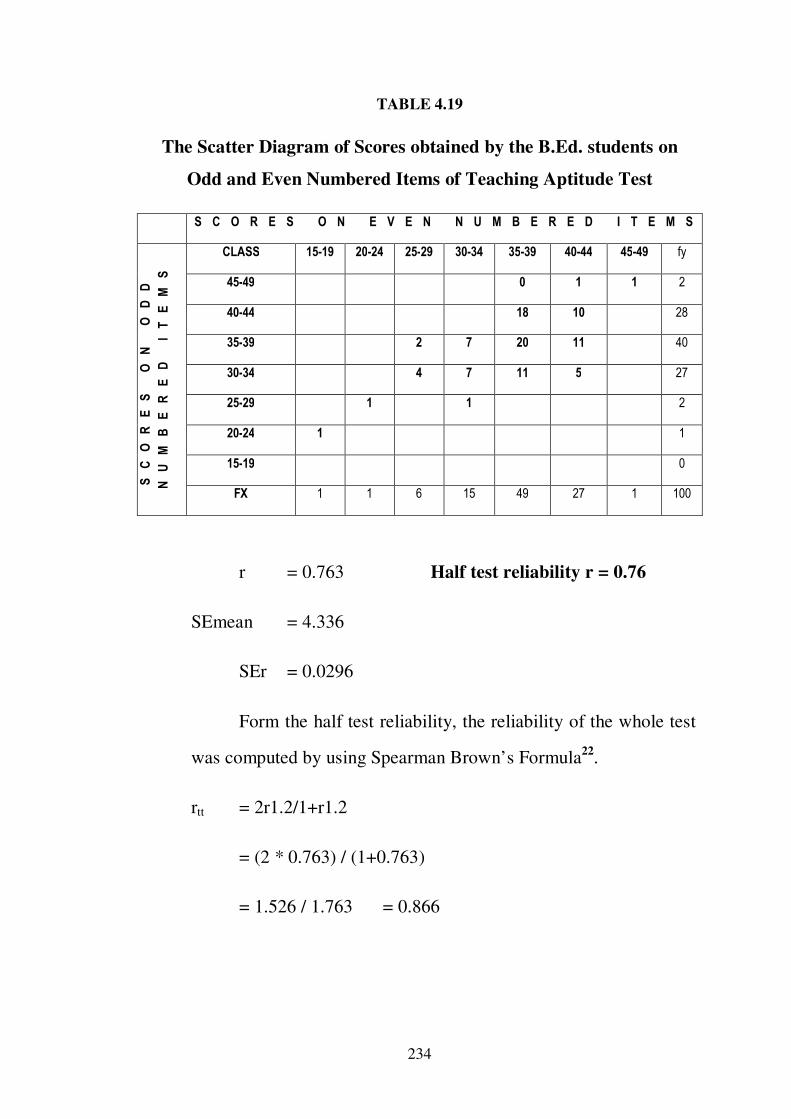
234

TABLE 4.19

The Scatter Diagram of Scores obtained by the B.Ed. students on

Odd and Even Numbered Items of Teaching Aptitude Test

S C O R E S O N E V E N N U M B E R E D I T E M S

SC

OR

ES

O

N

OD

D

NU

MB

ER

ED

I

TE

MS

CLASS 15-19 20-24 25-29 30-34 35-39 40-44 45-49 fy

45-49 0 1 1 2

40-44 18 10 28

35-39 2 7 20 11 40

30-34 4 7 11 5 27

25-29 1 1 2

20-24 1 1

15-19 0

FX 1 1 6 15 49 27 1 100

r = 0.763 Half test reliability r = 0.76

SEmean = 4.336

SEr = 0.0296

Form the half test reliability, the reliability of the whole test

was computed by using Spearman Brown’s Formula22

.

rtt = 2r1.2/1+r1.2

= (2 * 0.763) / (1+0.763)

= 1.526 / 1.763 = 0.866

235

The reliability of the whole test is high. It provides

indication that the test is quite reliable tool to measure Teaching

Aptitude of B.Ed. students.

The P.E. of the ‘r’ (0.87) was found as under,

SEmean = 4.336

P.E. ‘r’ = 0.042

4.4.2.3 Method of rational Equivalence :

This method was developed by Kuder and Richardson.

It is also known as K-R Method. This method is useful for

estimating the interval consistency or homogeneity of a test/scale.

The Kuder Richardson Formula was developed because of

dissatisfaction with split-half methods. A scale can be split into two

equal halves in great many ways and each split might yield

somewhat different estimate of rtt. The use of item statistics get

away from each basis as may arise from arbitrary splitting into

halves. Finally, the most accurate and practical formula was

developed as follows23

,

rtt = n/n-1 x σt2 - Σpq / σt

2

in which rtt = reliability coefficient of the whole test.

n = number of items in the test.

236

σt2 = the S.D. of the test scores.

P = the proportion of the group answering a test item

correctly.

Q = (1-p) = the proportion of the group answering a test

item incorrectly.

This formula is called Kuder and Richardson’s 20. Kuder

and Richardson formula 20 is applicable only to a tests in which

the items are scored by giving one point if answered correctly and

nothing if not answered correctly.

With regard to the above discussion, the formula K-R 20 was

applied for the estimation of the reliability of the present test. For

this, the 100 answer sheets were randomly selected maintaining all

the major characteristics of the whole sample.

The proportion of the group answering a test item correctly,

‘p’ was found out for each of the 118 test-items. From these values

of ‘p’ the values of corresponding ‘q’s were also found out.

In the Table No. 4.20, the value of ‘pq’ for each item is

given. The sum of all pq values is equal to 21.176.

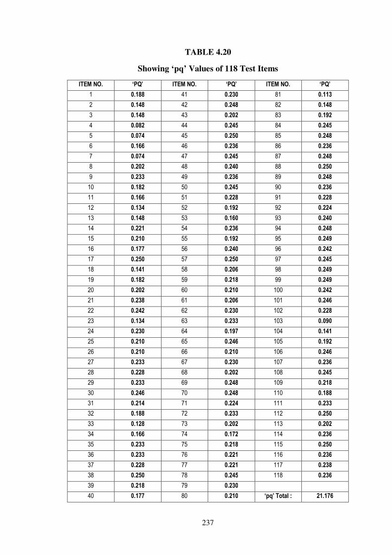
237

TABLE 4.20

Showing ‘pq’ Values of 118 Test Items

ITEM NO. ‘PQ’ ITEM NO. ‘PQ’ ITEM NO. ‘PQ’

1 0.188 41 0.230 81 0.113

2 0.148 42 0.248 82 0.148

3 0.148 43 0.202 83 0.192

4 0.082 44 0.245 84 0.245

5 0.074 45 0.250 85 0.248

6 0.166 46 0.236 86 0.236

7 0.074 47 0.245 87 0.248

8 0.202 48 0.240 88 0.250

9 0.233 49 0.236 89 0.248

10 0.182 50 0.245 90 0.236

11 0.166 51 0.228 91 0.228

12 0.134 52 0.192 92 0.224

13 0.148 53 0.160 93 0.240

14 0.221 54 0.236 94 0.248

15 0.210 55 0.192 95 0.249

16 0.177 56 0.240 96 0.242

17 0.250 57 0.250 97 0.245

18 0.141 58 0.206 98 0.249

19 0.182 59 0.218 99 0.249

20 0.202 60 0.210 100 0.242

21 0.238 61 0.206 101 0.246

22 0.242 62 0.230 102 0.228

23 0.134 63 0.233 103 0.090

24 0.230 64 0.197 104 0.141

25 0.210 65 0.246 105 0.192

26 0.210 66 0.210 106 0.246

27 0.233 67 0.230 107 0.236

28 0.228 68 0.202 108 0.245

29 0.233 69 0.248 109 0.218

30 0.246 70 0.248 110 0.188

31 0.214 71 0.224 111 0.233

32 0.188 72 0.233 112 0.250

33 0.128 73 0.202 113 0.202

34 0.166 74 0.172 114 0.236

35 0.233 75 0.218 115 0.250

36 0.233 76 0.221 116 0.236

37 0.228 77 0.221 117 0.238

38 0.250 78 0.245 118 0.236

39 0.218 79 0.230

40 0.177 80 0.210 ‘pq’ Total : 21.176

238

After analysing the responses of the B.Ed. students, sum of

‘pq’ for the whole test was found out. This value was substituted in

the following formula:

rtt

= 1.008

= 0.81

The reliability coefficient of the present aptitude test as

measured by K-R method is, therefore, 0.81. Hence, it is concluded

that the test is highly reliable.

TABLE 4.21

A Comparison of the Reliability Co-efficient of the Present Test

with four other Aptitude Tests

METHOD

APPLIED

SHAH

‘r’

SHRIVASTAV

‘r’

PANDYA

‘r’

UPADHYAYA

‘r’

PRESENT

TEST ‘r’

Test-Retest - 0.90 0.50 0.77 0.77

Split-half 0.88 - 0.63 0.81 0.76

K-R Formula-20 0.80 - - - 0.81

The above table 4.21 shows a comparison of the reliability

co-efficient of the present test with other aptitude tests.

239

Comparatively a high reliability can be seen in the test standardized

by the researcher.

4.4.2.4 Reliability in terms of True Scores and Measurement

Errors :

(a) Reliability co-efficient as a measure of true variance :

The variance of the obtained scores can be divided into two

parts : the variance of the true scores and the variance of chance

errors.

The reliability of the present test (K-R method) is 0.81.

therefore, 81 percent of the variance of test scores is true variance

and only 19 percent error variance.

(b) Estimating true scores by way of the regression

equation and the Reliability coefficient

The regression equation24

which estimates true score is given

below :

Where, = estimated true score on the test

= obtained score on the test

= mean of test distribution (73.36)

rtt = reliability coefficient of the test (0.81)

The regression equation for estimating true score on the

present test is worked out as under :

= (0.8*94) + 7.336

= 82.54

240

The standard error of an estimated true score is given by the

following formula25

,

SE∞ =

where, = 10.67

rtt = 0.81

The SE∞, of the true score on the present test is calculated

below :

= 10.67 x 0.3

= 3.20

The 0.95 confidence interval is

X∞ ± 1.96 x 3.20, i.e. π∞ ± 6.

(c) The index of reliability

The correlation between a set of obtained scores and their

corresponding true counterparts was found by finding the index of

reliability. For this, the following formula26

was employed.

where, r1∞ = the correlation between obtained and true scores

rtt = the reliability coefficient of the test

The coefficient r1∞ is called the index of reliability.

The index of reliability for the present test is :

= 0.90

241

Thus, 0.90 is the maximum correlation which the test is

capable of yielding in the present form.

4.5 Validity of the Test :

Tests should be held suspect until worth is proved, because the

tests that are supposed to measure intelligence, teaching aptitude,

adjustment etc. may not measure those characteristics at all. Edward E.

Cureton says, “The essential question of test validity is how well a test

does the job it is employed to do. The same test may be used for several

different purposes, and its validity may be high for one, moderate for

another and low for the third. Hence, we cannot label the validity of a test

as ‘high’ or ‘moderate’ or ‘low’ except for some particular purpose.”

Therefore, before a test can be used it is necessary to make certain

that the purpose of the test is justified. This leads us to the subject of test

validation. Validation of a test score is the most essential and the crux of

the process of standardization of any test, and it is also the most important

criteria to judge whether the test is good or poor. To justify the validity of

the test, it is necessary to clear, the concept of the term ‘validity’.

4.5.1 The Concept of Validity :

Validity is an important characteristic of the test. The

validity of the test depends upon the efficiency with which it

measures what it attempts to measure. Ti is also defined as the

accuracy with the test measures what it claims to measure. The

validity and the purpose of the test are closely associated. A test is

valid when it fulfils the purpose for which it was designed. The test

designed to test intelligence should measure only intelligence and

not any other thing. Similarly a test of teaching aptitude should

measure on teaching aptitude and not any other thing such as

242

intelligence or expression. Therefore, in case of valid teaching

aptitude test, the B.Ed. Students who are more capable for teaching

profession should get more scores than those who are weak.

Freeman defined it, as an essential index, “An index of validity

shows the degree to which a test measures what it proposes to

measure when compared with accepted criteria.”27

This suggests that for validating the test, it must be

compared with some accepted standards or other criteria which are

regarded by experts as the best evidence of the traits or ability to be

measured by the test. Therefore, the selection of validation criteria

is of prime importance in the process of the test validation.

4.5.2 Methods for Determining Validity :

Fundamentally, all procedures for determining the test

validity are concerned with the relationship between performance

on the test and other independently observable facts about the

behaviour characteristic under consideration. The technique that

are employed for investigating these relationships are numerous

and have been described by various names, “The APA Technical

Recommendations (i) classified these procedures under four

categories, defined as content, predictive, concurrent and construct

validity.”28

Out of these four categories of validity the two, namely

content and construct or concept validity are describe under the

heading of rational validity by many authors. Similarly, concurrent,

predictive and congruent validity are described under the heading

of empirical or statistical validity. In these methods the validity is

estimated by means statistical techniques.

243

The validity of the present test that has been established is

predictive validity.

(A) Content Validity :

Content validity has been decided on two groups, experts

opinion and validity index. Construction and item selection of test

has been already discussed at length in chapter – 3 of this report.

As for the validity index, items showing more than 0.20 validity

index have been selected and those below that have been rejected.

Concept validity has not been taken into account. Since this

test aspires to ascertain or test no concept and since there is no

other aptitude test of this type in Gujarati, congruent validity of the

test is out of question. Concurrent validity has not taken into

account.

(B) Predictive Validity :

Coefficient of validity of a test is the coefficient of

correlation between test scores and criterion scores. External

criteria for this test have been (scores) achieved at the University

examination of the B.Ed. degree.

The B.Ed. examination is being held in two parts: Part I –

Theory (700 marks) and Part II – Practical including Annual

Lesson (500 marks). For the present study the final percentage i.e.

the total of Part I and Part II, is considered as Academic

Achievement Scores.

It is possible that all the B.Ed. Students who had taken the

under report may not have taken their University examination or,

some of them have partly passed the same. With this possibility in

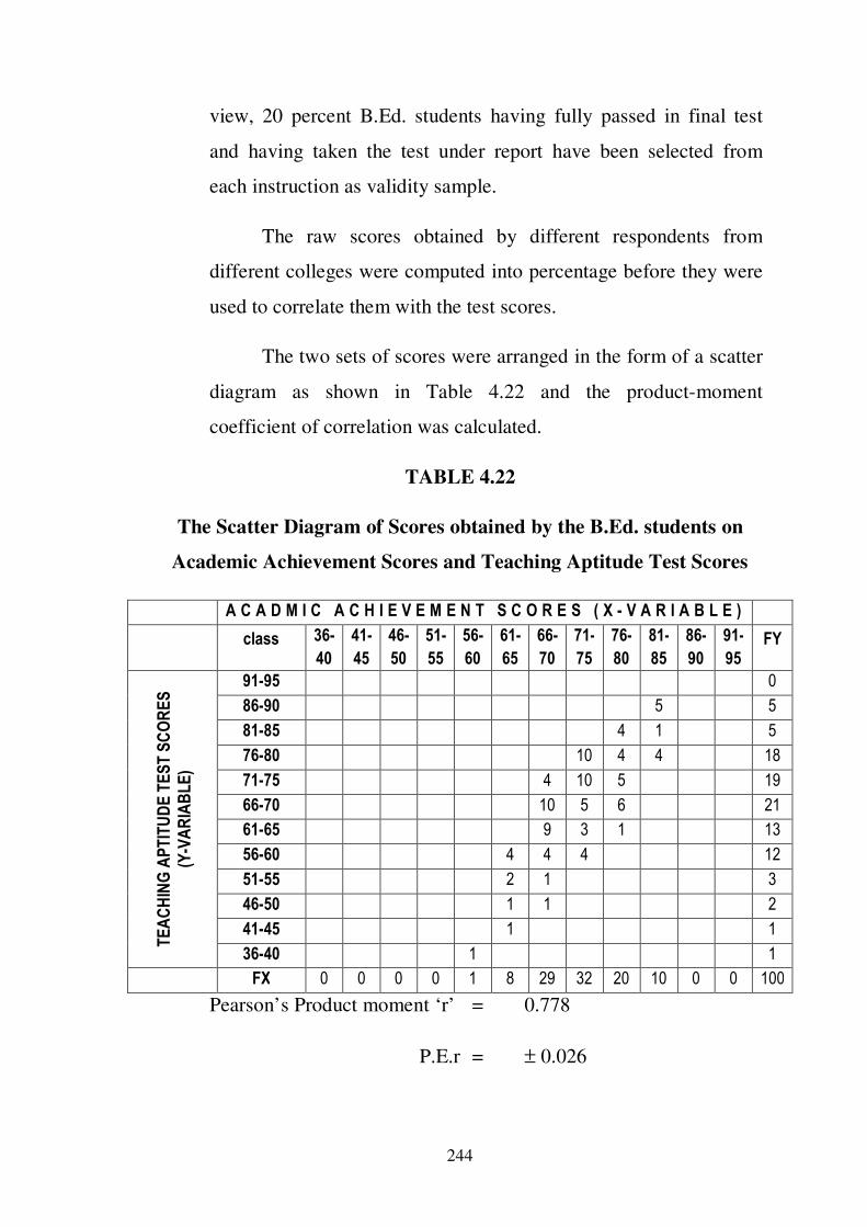
244

view, 20 percent B.Ed. students having fully passed in final test

and having taken the test under report have been selected from

each instruction as validity sample.

The raw scores obtained by different respondents from

different colleges were computed into percentage before they were

used to correlate them with the test scores.

The two sets of scores were arranged in the form of a scatter

diagram as shown in Table 4.22 and the product-moment

coefficient of correlation was calculated.

TABLE 4.22

The Scatter Diagram of Scores obtained by the B.Ed. students on

Academic Achievement Scores and Teaching Aptitude Test Scores

A C A D M I C A C H I E V E M E N T S C O R E S ( X - V A R I A B L E )

class 36-

40

41-

45

46-

50

51-

55

56-

60

61-

65

66-

70

71-

75

76-

80

81-

85

86-

90

91-

95 FY

TEA

CH

ING

APTIT

UD

E T

EST S

CO

RES

(Y-V

AR

IAB

LE)

91-95 0

86-90 5 5

81-85 4 1 5

76-80 10 4 4 18

71-75 4 10 5 19

66-70 10 5 6 21

61-65 9 3 1 13

56-60 4 4 4 12

51-55 2 1 3

46-50 1 1 2

41-45 1 1

36-40 1 1

FX 0 0 0 0 1 8 29 32 20 10 0 0 100

Pearson’s Product moment ‘r’ = 0.778

P.E.r = ± 0.026

245

The Teaching Aptitude Test predicts the criterion

significantly well, because the test and Part I correlation is 0.778.

This means the present test is valid instrument for predicting

Teaching Aptitude.

4.6 Conclusion :

In this chapter the researcher has presented the process of

standardization of the tool –Teaching Aptitude Test. The Reliability and

Validity calculated for the tool standardized was high. The Norms

establishment was the second most important part of this chapter. To

standardize the test the researcher had administered the tool following the

three steps – Pre-Pilot, Pilot, and Final test. The administration and

results of Pre-Pilot Test, Pilot Test and Final Test of Teaching Aptitude

Test were also discussed in the beginning of the chapter. The analysis and

interpretation of the data as discussed in the following chapter would

support the Norms establishments for the tool standardized.

246

REFERENCES

1. Garret H.E. (1968). General Psychology (Second Edition).

New Delhi : Eurasia Publishing House (Pvt.) Ltd. Ram

Nagar. PP. 486-488

2. Anne Anastasi. (1970). Psychological Testing. New Delhi :

Macmillan Pub.

3. Guilford, J.P. (1956). Fundamental Statistics in Psychology

and Education (Fourth Edition). New York : McGraw

Hill Book Co.

4. Green J. Gerberich. (1957). Measurement and Evaluation in

Secondary School. New York : Longmans Green and

Co.P.93

5. Ibid. P.90

6. Summer, S.P. (1954). Statistics in Education. London : Bacil

Blackwell and Co.

7. Garret H.E. (1968). General Psychology (Second Edition).

New Delhi : Eurasia Publishing House (Pvt.) Ltd. Ram

Nagar.

8. Walker H.M. and Lev J. (1965). Statistical Inference. Calcutta : Oxford &

IBH Pubshing Co. PP. 472-475

9. Ross, C.C. and Stanely, J.C. (1963). Measurement in Today’s School.

New Jersey : Prantice Hall, Inc. P.122

10. Garret H.E. (1981). Statistics in Psychology and education.

(10t h

Edition). Bombay : Vakils, Feffer and Simons Ltd.

P. 100

11. Ibid, P.241

12. Ibid, P.100

13. Ibid, P.242

247

14. Ibid, PP. 312-313

15. Ibid, PP. 315-317

16. Ibid, PP. 67-68

17. Lado, Robert (1962). Language Teaching – The Construction and Use of

Foreign Language Tests : A Teacher’s Book. London : Longman

Green and Co. Ltd. P.330

18. Mehrens, W.R. and lehmann, I.J. (1969). Standardized Tests in

Education. New York : Holt, Rinhart and Winston Inc. P.32

19. Anne Anastasi, Op.Cit. P.71

20. Freeman Frank S. (1967), Theory and Practice of Psychology of

Testing. New York : Harper and Raw. P.67

21. Rulon, P.J. (1039). A simplified Procedure for Determining the

Reliability of a Test by Split-halves. Haward Education. Review.

Vol-IX.

22. Ibid, P.339

23. Ibid, P.341

24. Ibid, PP. 347-348

25. Ibid, PP. 347-348

26. Ibid, P. 349

27. Freeman, F.S. Op. Cit. P.26

28. Anne Anastasi, Op.Cit. P.135