
4. Forced Convection Heat Transfer Library/20043805.pdf · 4.1 Page 4.2 4. Forced Convection Heat...
84
4.1 4.1.1 4.1.2 4.1.3 4.2 4.2.1 4.2.1.1 4.2.1.2 4.2.2 4.3 4.3.1 4.3.1.1 4.3.1.2 4.3.2 4.3.2.1 4.3.2.2 4.4 4.4.1 4.4.1.1 4.4.1.2 4.4.1.3 4.4.2 4.4.2.1 4.4.2.2 4.4.2.3 4. Forced Convection Heat Transfer Fundamental Aspects of Viscous Fluid Motion and Boundary Layer Motion Viscosity Fluid Conservation Equations- Laminar Flow Fluid Conservation Equations - Turbulent Flow The Concept pf Boundary Layer Laminar Boundary Layer Conservation Equations - Local Formulation Conservation Equations -Integral Formulation Turbulent Boundary Layer Forced Convection Over a Flat Plate laminar Boundary Layer Velocity Boundary Layer - Friction Coefficient Thermal Boundary Layer- Heat Transfer Coefficient Turbulent Flow Velocity Boundary Layer - Friction Coefficient Heat Transfer in the Turbulent Boundary Layer Forced Convection In Ducts laminar Flow Velocity Distribution and Friction Factor In Laminar Flow Bulk Temperature Heat Transfer in Fully Developed Laminar Flow Turbulent Velocity Distribution and Friction Factor Heat Transfer In Fully Developed Turbulent Flow Non- Circular Tubes Page 4.1
Transcript of 4. Forced Convection Heat Transfer Library/20043805.pdf · 4.1 Page 4.2 4. Forced Convection Heat...

4.1
4.1.1
4.1.2
4.1.3
4.2
4.2.1
4.2.1.1
4.2.1.2
4.2.2
4.3
4.3.1
4.3.1.1
4.3.1.2
4.3.2
4.3.2.1
4.3.2.2
4.4
4.4.1
4.4.1.1
4.4.1.2
4.4.1.3
4.4.2
4.4.2.1
4.4.2.2
4.4.2.3
4. Forced Convection Heat Transfer
Fundamental Aspects of Viscous Fluid Motion and Boundary
Layer Motion
Viscosity
Fluid Conservation Equations - Laminar Flow
Fluid Conservation Equations - Turbulent Flow
The Concept pf Boundary Layer
Laminar Boundary Layer
Conservation Equations - Local Formulation
Conservation Equations -Integral Formulation
Turbulent Boundary Layer
Forced Convection Over a Flat Plate
laminar Boundary Layer
Velocity Boundary Layer - Friction Coefficient
Thermal Boundary Layer - Heat Transfer Coefficient
Turbulent Flow
Velocity Boundary Layer - Friction Coefficient
Heat Transfer in the Turbulent Boundary Layer
Forced Convection In Ducts
laminar Flow
Velocity Distribution and Friction Factor In Laminar Flow
Bulk Temperature
Heat Transfer in Fully Developed Laminar Flow
Turbulent
Velocity Distribution and Friction Factor
Heat Transfer In Fully Developed Turbulent Flow
Non- Circular Tubes
Page 4.1

4.1
Page 4.2
4. Forced Convection Heat Transfer
In Chapter 3, we have discussed the problems of heat conduction and
used the convection as one of the boundary conditions that can be applied to
the surface of a conducting solid. We also assumed that the heat transfer rate
from the solid surface was given by Newton's law of cooling:
q" =h,A~w-tJ
In the above application, he' the convection heat transfer coefficient has been
supposed known. The aim of this chapter is to discuss the basis of heat
convection in fluids and to present methods (correlations) to predict the value of
the convection heat transfer coefficient (or film coefficient).
As already pointed out. the convection is the term used to indicate heat
transfer which takes place in a fluid because of a combination of conduction due
to molecular interactions and energy transport due to the motion of the fluid
bulk. The motion of the fluid bulk brings the hot regions of the fluid into contact
with the cold regions. If the motion of the fluid is sustained by a force in the form
of pressure difference created by an external device, pump or fan, the term of
"forced convection is used". If the motion of the fluid is sustained by the
presence of a thermally induced density gradient. then the term of "natural
convection" is used.
In both cases, forced or natural convection, an analytical determination
of the convection heat transfer coefficient. he' requires the knowledge of
temperature distribution in the fluid flowing on the heated surface. Usually, the
fluid in the close vicinity of the solid wall is practically motionless. Therefore, the
heat flux from the solid wall can be evaluated in terms of the fluid temperature
gradient at the surface:
qll = -k (!!!-)cv Idn s 4.2

Page 4.3
where
kf : thennal conductivity of the fluid
(.E!.) :fluid temperature gradient at the surface in the direction of the normal to the surfacedn s
The variation of the temperature in the fluid is schematically illustrated in Figure
4.1. Combining Equations 4.1 and 4.2 we obtain:
4.2a
where
tw : temperature of the wall
tf : temperature of the fluid far from the wall
(01)oy ..
Figure 4.1 Variation of the temperature in the fluid next to the heated surface
The analytical determination of he given with Equation 4.2a is quite
complex and reqLires the solution of the fundamental equations governing the

Page 4.4
motion of viscous fluid; equations of conservations of mass, momentum and
energy. A brief discussion of these equations was given in Chapter 2.
4.1 Fundamental Aspects of Viscous Motion and Boundary Layer
Motion
4.1.1 Viscosity
F
u
,/
I
ei
Fix woI!
t---..----
The nature of viscosity is best visualized with the following experiment.
Consider a liquid placed in the space between two plates, one of which is at
rest, the other moves with a constant velocity U under the effect of a force F.
The experimental setup is illustrated in Figure 4.2.
U
Figure 4.2 Shear stress applied to a fluid
The distance between the plates is e and the surface area of the upper
plate in contact with liquid is A. Because of the non-slip cond ition, the fluid
velocity at the lower plate is zero and at the upper plate is U. Assuming that the
Couette flow conditions prevail (ie, no pressure gradient in the flow direction) a
linear velocity distribution, as shown in Figure 4.1, develops between the plates
and is given by:
Uu=-y
e 4.3

4.4
Page4.5
The slope of this distribution is constant and given by:
du Udy=~
The shear stress exerted by the plate to the liquid is written as:
FT=-
A
It is possible to repeat the above experiment for different forces (i.e.
upper plate velocities) and plot the resulting shear stress, T, versus the slope of
the velocity distribution (du Idy). Such a plot is shown in Figure 4.3.
10<::.. -.
du/dy
Figure 4.3 T versus (du Idy)
Data points lie on a straight line that passes through the origin. Therefore T is
proportional to the velocity gradient, (du Idy) and the constant of proportionality
is J1. J1 is called the "dynamic viscosity". Based on the above discussion, the
shear stress can be written as:
duT=J1-
dy 4.5
In a more general way, consider a laminar flow over a p lane wall. The velocity
of the fluid is parallel to the wall and varies from zero to some value far from the

Page 4.6
wall. The velocity distribution close to the wall, as depicted in Figure 4.4 is not
linear.
s
o
u
duV4Y
11- S~-
,A
~Tf u
Figure 4.4 Velocity distribution next to a wall
Let us select a plane SS parallel to the wall. The fluid layers on either side of SS
experience a shearing force '!' due to their relative motion. The shearing stress,
'!', produced by this relative motion is again directly proportional to the velocity
gradient in a direction normal to the plane SS:
1: =J1(dU)dy ss
The ratio of the dynamic viscosity to the specific mass of the fluid
v=l!:.p
is called "kinematic viscosity"
The dynamic viscosity has dimensions:
1: F T FTJ1 = du =L' ZL=lf
dy
4.6
4.7
4.8
F,L,T are force, length and time, respectively. In the Sf, the dimensions of the
dynamic viscosity becomes:

Page 4. 7
NsJl=m2
The dimensions of the kinematic viscosity are:
L2
v=-T
or in Sf units
m'v=
s
The physical basis of viscosity is the momentum exchange between the
fluid layers. To understand better this statement, consider one dimensional
laminar flow of a dilute gas on a plane wall as depicted in Figure 4.5. The
velocity of the fluid U is only a function of y. Let us imagine in the flow a
surface SS parallel to the plane wall.
y
uo
-+-+----t'----i---E!-'A u(y+:A.}
s--+-+-+~;t;.=-++fA~U~Y_:A.)
1"6 nI1mu(y + A.)
u
1- nI1mu(y - A.)6
Figure 4.5 Momentum exchange by molecular diffusion
Because of the random thermal velocities, gas molecules continually
cross the SS surface both above and below. We may assume that the last
collision before crossing the surface SS, each molecule acquires the flow
velocity corresponding to the height at which this collision has taken place.
Page 4.8
Since this velocity above the 55 is greater than that below, molecules crossing
from above transport a greater momentum in the direction of the flow across the
surface than that transported by the molecules crossing the same surface from
below. The result is a net transport of momentum across the surface 55 from
the region above to the region below. According to the Newton's second law,
this change of momentum is balanced by the viscous force. This is the reason
for which the region of gas above 55 is submitted to a force which is due to the
region of the gas below 55 (- T) and vice versa ( T).
We will try now to estimate in an approximate manner the dynamic of
viscosity 11. If there are m molecules per unit volume of the dilute gas,
approximately 1/3 of these molecules have an average velocity ( v) parallel to
1the y-axis. From these molecules. half of them (ie. 6n
) have an average
velocity in the direction of Y' and the other half have an average velocity in the
1 -direction of Y-. Consequently. an average 6nv molecules cross the plane 55
per unit surface and per unit time from above to below and vice versa.
Molecules coming from above 55 undergo their last collision at a distance
approximately equal to the mean free path A and their flow velocity is tis + A)
and their momentum is mti•.Y + A) where m is the mass of the molecule. The
same argument is also true for molecules coming from below the surface 55
and their velocity is tis - A) and momentum mtis -A). Therefore. the
momentum component in the direction of the flow that crosses the surface 55
from above to below is:
inv [mu(Y+A)] 4.9
and from below to above:
-t Ii· rNvdA - Lii· pJdA+Lii~dA =0 in\' [mu(y -A)] 4.10

4.12
Page 4.9
The net momentum transport is the difference between Eqs 4.10 and 4.9 and
according to the Newton's second law should be balanced by a viscous force. r.Therefore we may write:
r =1nvm[u(y - A)- (y + A)]6 4.11
Developing u(y - A) and u(y + A) in Taylor series and neglecting the terms of
second and higher orders, we obtain:
duu(Y +A):o u(y )+A dy
u(Y-A):oU(Y)-A:
Substitution of Eqs 4.12 and 4.13 into 4.11 yields.
1 _ du dur=--nvmA-= -tJ.-
3 dy dy
4.13
4.14
The negative sign shows that the viscous stress acting on the upper face of 55
surface is in the direction opposite to the flow direction (or X'). From 4.14 we
observe that:
1 _ ,tJ. =-nvm"3
Although the constant 1/3 may not be correct. the dependence of tJ. on
11, v.m and A should be rather correct.
4.1.2 Fluid Conservation Equations- Laminar Flow
4.15
We have already pointed out that the analytical determination of the
convection heat transfer coefficient defined with Eq. 4.2 requires the solution of
the fluid conservation equations: mass, momentum and energy to obtain the
temperature distribution in the fluid washing the heated solid. Once the

Page 4.10
temperature distribution is determined and if the fluid motion in the region
immediately adjacent to the heated wall ;s laminar, which is usually the case, the
convection heat transfer coefficient is then determined by using Eq. 4.2. The
derivation of the fluid conservation equations is beyond the objective of this
course. We will present within the framework of this course, the basic elements
which enter in the derivation of the conservation equations and present these
equations for an incompressible flow.
In Chapter 2, we have already established that the fluid conservation
equations have the following forms:
I) Local mass conservation equation
a -aT P+V.pV =0
II) Local momentum conservation equation
a - - - --aTpV +VpVv =VpI + V·O' +pg
III) Energy conservation equation (total energy in enthalpy form)
.2.- j h + l v' v)_.2.- P+ ",.1h + lv· v)vaT i1... 2 aT i1... 2
= -Y'. q' +V'. f v)+ pg' V+ d;
In the above equation:
1 0 ~l:,; is the unit tensor = 0 1
o 0
(J~ (J", (Ju
C; is the stress tensor = (Jy, (J" (Jy,
(Ju (J"! (Ju
2.6
4.7
4.8

Page 4. 11
h enthalpy
p pressure
v velocity ( u,v,w are components of the velocity vector)
p specific mass
g acceleration of gravity
iT: heat flux
Q';: energy generation
Each term of the stress tensor can be related to the velocity gradients as follows
(Janna, 1986)
Furthermore we know that~
ij'=-kV·/
Assuming that
1. The fluid is incompressible and has constant properties, i.e.,
c p' p, Jl. and k are constant,
2. The kinetic energy and potential energies are negligible,
4.9
4.10
4.11
4.12
4.13
4.14
4.15

Page 4. 12
ap3. The pressure doesn't change with time, ar =0
4. No energy generation (f, =0,
and taking into account Eq. 4.9 through 4.15, the conservation equations (Eq's
4.6,4.7 and 4.8) become:
1. Mass conservation equation
au av Ow-+-+-=0ax ay ()z
11. Momentum conservation equation
x-component
~au au au au) ail ~()2U a'u ()2u)-+u-+v-+w- =-=+ -+-+- +pgar ax ay az ax ax' ay' az' x
y-component
j av av av av)_ l!E .ra'v a'v a'v)1\ar + u ax +vay + W az - - ay +1.ax' + Oy' + az' + Pfi,
z-component
~Ow Ow Ow Ow) ail (a'w a'w a'w)-+u-+v-+w- =-=+J.l -+-+- +pgar ax Oy az az ax' ay' az' ,
where
,,~(a)' (av)' (Ow),] (a CIv)' (av Ow)' (Ow a)'1/1= La; + ()y + az + ~ + at + az + ay + ax + a;
4.16
4.17
4.18
4.19
4.20
J1I/) is the viscous dissipation term, it is usually negligible compared to heat
transferred. Eqs. 4.17 through 4.19 are known as Navier-Stokes equations. In

Page 4.13
the problems of heat convection is a three-dimensional incompressible laminar
flow, the energy equation (Eq. 4.20) must be solved to obtain the temperature
distribution in the fluid. However, this equation contains the three components
of the velocity and its solution can only be carried out in conjunction with the
mass conservation equations and Navier·Stokes equations for a given set of
boundary conditions: shape and temperature of the heated body over which the
fluid flows, the fluid velocity and temperature far from the body, etc. For the
incompressible and constant property fluid we selected the unknown quantities
are: u, v, w, p and t. There are five equations: 4.16 through 4.20 to determine
these unknowns. Once the temperature distribution in the fluid is known, the
convection heat transfer coefficient at a given point on the heated surface can
be determined with the aid of Eq. 4.2.
It should be pointed out that the basic equations that govern the
convection are non-linear and are among the most complex equations of applied
mathematics. No general mel10ds are available for the solution of these
equations. Analytical solutions eXist for very simple cases. In recent years, with
the advent of high-speed and high-capacity computers, a good deal of progress
has been made in the analysis of complicated heat transfer problems. However,
these analysis is time consuming and very costly. Fortunately, a large number
of engineering problems can be adequately handled by using simplified forms of
the conservation equations, ie., by using a one dimensional model and
experimentally determined constitutive equations such as friction and heat
transfer coefficients. The solution of these simplified forms can be obtained
more easily. On the other hand, the soundness if the assumptions made to
obtain the simplified forms of the conservation equations should be verified by
ad-hoc experiments.
The conservation equations derived above apply to a laminar fluid
motion. In laminar flows, the fluid particles follow well-defined streamlines.
These streamlines remain parallel to each other and they are smooth. Heat and

Page 4.14
momentum are transferred across the streamlines (or between the adjacent fluid
layers which slide relative to one another) only by molecular diffusion as
described in Section 4.1. Therefore, the cross flow is so small that when a
coloured dye is injected into the fluid at some point, it follows the streamline
without an appreciable mixing. Laminar flow exists at relatively low velocities.
4.3 Fluid Conservation Equation - Turbulent Flow
The term turbulent is used to indicate that there are random variations
or fluctuations of the flow parameters such as velocity, pressure and arid
temperatures about a mean value. Figure 4.6 illustrates, for example, the
fluctuations of the u component of the velocity oblained from a hot-wire
anemometer.
II
L-L--+-....r.-------=i-limo---t..~a'ta
Figure 4.6 Turbulent velocity fluctuations about a time average.
If we denote by u the time average velocity and by u'
the time dependent velocity fluctuation about that average value, the true
velocity may be written as:
u= U+u'
The same reasoning may also be done for two components and write:
4.21

4.24
4.25
Page 4.15
v =v +v' 4.22
w= w+ w' 4.23
Because of these randomly fluctuating velocities. the fluid particles do
not stay in one layer but move tortuously throughout the flow. This means that a
certain amount of mixing and energy exchange occurs between the fluid layers
due to the random motion of fluid particles. This type of mixing is nOrHlxistent in
laminar flows and is of great importance in heat transfer problems since the
random motion of the particles tend to increase the rate of heat exchange
between the fluid layers. As a matter of fact. the rate of heat transfer is
generally much higher in turbulent flows than in laminar flow. Turbulent flow
exists at velocities that are much higher than in laminar flow. As a final note, the
pressures and temperatures in turbulent flows are written as:
p= p+ p'
The average values appearing in Eqs. 4.21 through 4.25 for steady turbulent
motion are given by:
- 1 SM,j = t1'f
1
0 jdr, independent of time for steady flows4.26
The time interval M, is taken large enough to exceed amply the period of the
fluctuations. On the other hand, the time average of the fluctuations, j'is zero:
- I rA', ISM", -\J - -I'=-j, j'd'f=- V -jp'f=j-j=O
t1'f1 0 t1'f1 0
In the above discussion j may denote any flow parameter.
4.27
To obtain the fluid conservation equations which apply to a turbulent flow. we
substitute in Eqs. 4.16 through 4.20, u,v, w,p and t by Eqs. 4.21,4.22,4.23.
4.24 and 4.25 respectively. Since in most of the convection problems the
viscous dissipation is negligible. this term can be dropped from the energy
conservation equation (Eq. 4.20). The next step consists of time averaging of
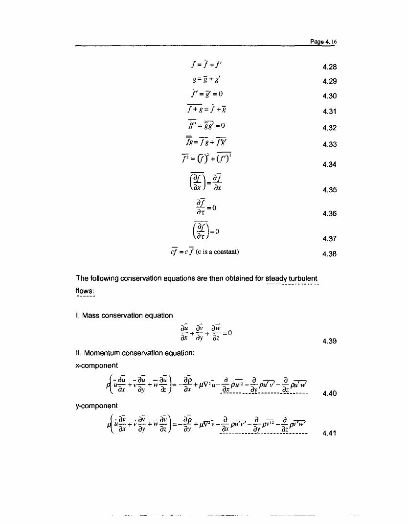
the resulting equations by taking into account the following averaging rules:
Page 4, 16
f=i+/' 4.28
g=g+g,
4.29
/,=g=O 4,30
f+g=f+g 4.31-.ff' =gg' =0 4,32
fg= Ti+ f'g' 4.33
f' =(i)' +(/')'4.34
(af)= atax ax 4.35
ll-oar- 4.36
(~)=O4.37
cf =c f (c is a constant) 4.38
The following conservation equations are then obtained for steady turbulent-----------------
flows:
I. Mass conservation equation
au aV aw-+-+-=0ax ay azII. Momentum conservation equation:
x-component
{-a; -a; -a;) an - a - a -,-, a -,-,u- +v- +w- =_::L+JI.'V'u--pu 12 _-pu V - -pu wax ay (£ ax A~ ib: qL _
y-component
{-av -av -av) an - a -, a li a -,-,u-+v-+w- =-=+Jl.V'v--pu'v --pv --pvwax dy az ay _~ q1: __ • q~ _
4.39
4.40
4.41

Page 4.17
z-eomponent
{- riW -aw - aw) ap - a -,-, a =-> au-+v-+w- =-- +J/.v'w--pu w --pvw --(iW12ax ()y az az _q:.r ~ qL __
III. Energy conservation equation
(- ai -ai -ai) a - a - a -IX' u-+v-+w- =kV't- -IX' u't'-- IX' v'f -- pc wt'p ax ay az ~ __: }y : ~~. __p _
where
4.42
4.43
4.44
Examination of the about equations shows that the usual steady equations (Eq.
au av aw and ~4.16 through 4.20 with ar' ar' ar arterms equal zero) may be applied to
the mean flow provided certain additional terms are included. These terms,
indicated by dashed underli nes and they are associated with the turbulent
fluctuations. The fluctuating terms appearing in Eq. 4.40 to 4.42 represent the
components of the "turbulent momentum flux" and they are usually referred to
as additional "apparent stresses" or "Reynold stresses" resulting from the
turbulent fluctuations. The fluctuating terms appearing in Eq. 4.43 represent the
components of "the turbulent energy flux". A discussion of the meaning of
"apparent stresses" and "turbulent energy flux" will be done during the study of a
flow over a heated wall.
4.2 The Concept of Boundary Layer
Let us consider the flow of viscous fluid over a plate, as illustrated in Fig. 4.7.

Page 4.18
yu
x,u
Figure 4.7 Velocity profile in the vicinity of a plate
The velocity of the fluid far from the plate (free steam velocity) is U. If the basic
"non slip" assumption is made then the fluid particles adjacent to the surface
adhere to it and have zero velocity. Therefore, the velocity of fluid close to the
plate varies from zero at the surface to that of the free stream velocity, U.
Because of the velocity gradients, viscous stresses exist in this region and their
magnitude increases as we get closer to the wall. The viscous stresses tend to
retard the flow in the regions near to the plate.
Based on the above observations, LUdwig Prandtl, in 1904 proposed his
boundary layer theory. According to Prandtl, the motion of a fluid of small
viscosity and large velocity over a wall could be separated into two distinct
regions:
1. A very thin layer (known as velocity boundary layer) in the immediate
neighbourhood of the wall in which the flow velocity ( U) increases rapidly with
the distance from the wall. In this layer the velocity gradients are so large that
even with a small fluid viscosity, the product of the velocity gradient and the
viscosity (ie. the viscous stress, 'l") may not be negligible.
2. A potential flow region (or potential core) outside the boundary layer were the
influence of the solid wall died out and the velocity gradients are so small that
the effect of the fluid viscosity. ie. the viscous stress, 'l", can be ignored.
Page 4.19
A good question would be: where is the frontier between these two regions
situated? The answer is that, because of the continuous decrease of the
velocity as we move off the wall, it is not possible to define the limit of the
boundary layer and the beginning of the potential region. In practice, the limit of
the boundary layer ie., the boundary layer thickness, is taken to be the distance
to the wall at which the flow velocity has reacted some arbitrary percentage of
the undisturbed free stream velocity. 99% of the free stream velocity is the most
often used criterion.
4.2.1 Laminar Boundary Layer
The flow in the boundary layer is said to be laminar where fluid particles move
along the streamlines in an orderly manner. The criterion for a flow over a flat
plate to be laminar is that a dimensionless quantity called Reynolds number,
Re u ' and defined as:
pUxRex =--
f..l 4.45
should be less than 5 x 10⁵. The number is the ratio of the inertia forces to the
viscous forces.
The analytical study of the boundary can be conducted by using:
1. The fluid equations given by Eqs. 4.16 through 4.20, or
2. An approximate method based on integral equations of momentum and
energy.
The integral method describes, approximately, the overall behaviour of the
boundary layer. The derivation of the integral fluid equation will be given in this
section. Although the results obtained by the integral approach are not
complete and detailed as the results that may be obtained by the application of

Page 4.20
the differential equations, this method can still be used to obtain reasonable
accurate results in many situations.
4.2.1.1 Conservation Equations - Local Formulation
I. Mass and Momentum Equations
As a simple example, consider the flow and heat transfer on a flat plate as
illustrated in Figure 4.8.
Potentialllow regionU(x),
P.(x).
I,
. 'to
]I LConIrQlwlwnc
o ~X,II,I
........ -----
Velocitylayer
Figure 4.8 Velocity boundary layer in Laminar flow near a plane.
The x coordinate is measured parallel to the surface starting from leading edge.
and the y coordinate is measured normal to it. The velocity and the pressure of
the fluid far from the plate are U(x) and p~ (x), respectively; usually they are
constant. The leading edge of the plate is Sharp enough not to disturb the fluid
flowing in the close vicinity of the plate. The boundary layer starts with the
leading edge of the plate and the thickness is a function of the coordinate x.
The thickness of the boundary layer is denoted by t5(x).

Page 4.21
Assuming that the flow field is steady and two dimensional (ie., no velocity and
temperature gradients in Z direction which is perpendicular to the plane of the
sketch), body forces P8x and P8y are negligible compared to the other terms,
Eqs 4.16 through 4.19 become:
Mass conservation equation:
au av-+-=0ax ay
Momentum conservation:
au au _.!.2e ((fU a'u)uax+Vay--pa:+v ax'+ay"
4.46
4.47
4.48
4.50
The coefficent v (m2/s) is the kinematic viscosity of the fluid. Even with the
above simplifications, Eqs 4.46 through 4.48 are still non-linear and cannot be
solved analytically.
An order of magnitude analysis of each term of Eqs. 4.46, 4.47 and
4.48 shows that the following terms (Schlichting, 1979)
a'u av av a'v a'v a'u av av a'v a'vv <tt' ,uax'v ay'V ax' and v ay' v <tt' .uax'v ay'V ax' and v ay'
are very small and can be ignored. Therefore, Eqs 4.46 through 4.48 become
au + av =0ax ()y 4.49
~ v au __LEi! a'uar + ()y - p ax + v ay'
4.51
Eq. 4.51 shows that, at a given x, the pressure is constant in the y -direction,
ie., it is independent of y. This result implies that the pressure gradient,

Page 4.22
dp /dx dp /dx , in the boundary layer, taken in a direction parallel to the wall, is
equal to the pressure gradient potential flow taken in the same direction. The
boundary conditions that apply to Eqs. 4.49 and 4.50 are:
Aty =0 u= v= 0
Aty =00 u =U(x) which is usuallycoostant
4.52
4.53
4.54
The solution of Eqs. 4.49 and 4.50 under the above boundary conditions yields
the velocity distribution and the boundary layer thickness. However, this
solution is beyond the scope of this course; it can be found in Scl1ichting (1979)
at pages 135·140.
At the outer edge of the velocity boundary layer the component of the
velocity parallel to the plate, n, becomes equal to that ofthe potential flow, U(x)
Since there is no velocity gradient in this region;
du d 2u-=Oand -=0dy dy2
and Eq. 4.50 becomes
dU(x) 1 dpU(x)--=---
dX pdx
Integrating the above equation we obtain:
1p+ - pU2(X)= Constant
2
This is nothing else but the Bernoulli equation.
4.55
4.56
II. Energy conservation equation
If the temperature of the plate ( tw ) is different from the temperature of
the mainstream ( t_), a thermal boundary layer of thickness 5, forms. Through
the layer of the fluid temperature makes the transition from the wall temperature
to the free stream temperature. The thickness of the thermal boundary layer is
in the same order of magnitude as the velocity boundary layer thickness defined
4.57
Page 4.23
above. However, the thicknesses of both boundary layers are not necessarily
equal (Figure 4.8).
For a two dimensional flow where viscous terms have been neglected in
comparison with the heat added from the wall, the energy equation given by Eq.
4.20 for steady state conditions takes the following form
u2!..+v2!..=~. (a2t+ a2
t)ax ()y pcp ax 2 ay2
An order of magnitude analysis shows that the term
a'tax'
a'tIs very small and can be ignored compared to ()y'. Therefore Eq. 4.55
becomes:
at at a'tu-+v-=a-ih: ay' ay2
4.58
k fa=-where pe P. For a constant temperature wall, tw , the applicable boundary
conditions are:
y=o t= tw 4.59
y=oo t=c 4.60
x=o t=c 4.61
The solution of Eq 4.58 in conjunction with Eqs 4.49 and 4.50 subject to
boundary conditions given by Eqs 4.52,4.53 and 4.59 through 4.61 yields the
temperature distribution and the thickness of the thermal boundary layer defined
with the same criterion as the velocity boundary layer. The knowledge of the
temperature distribution in the thermal boundary layer allows us to determine in
conjunction with Eq 4.2 the convection heat transfer coefficient, h.

Page 4.24
4.2.1.2 Conservation Equations - Integral Formulation
One of the important aspects of boundary layer theory is the
determination of the shear forces acting on a body and the convective heat
transfer coefficient if the temperature of the wall is different from that of the free
stream. As was discussed in the previous section, such results can be obtained
from the governing equation for laminar boundary layer flow. We also pointed
out that the solutions of these equations were quite difficult and were not within
the scope of the present course. In this section, we will discuss an alternative
method called "integral method" to analyze the boundary layer and to determine
the shear stress and the convection heat transfer coefficient. The use of this
method simplifies greatly the mathematical manipulations and the results agree
reasonably well with the results of exact solutions.
The integral method of analyzing boundary layers, introduced by Von
Karman (1946), consists of fixing the attention on the overall behaviour of the
layer as far as the conservation of mass, momentum and energy principles are
concerned rather than on the local behaviour of the boundary layer.
In the derivation of the integral boundary laye r equation, the integral
conservation equations given in Chapter 2, Eqs 2.21, 2.22, and 2.33 will be
used. These equations for a fixed control volume (ie., IV =0) and under steady
state flow conditions have the following forms:
Mass conservation:
Momentum conservation (volume forces (I.e. gravity) are neglected:
-L "'pVvdA-Ln. pldA+L"~dA=O
Energy equation (enthalpy form):
Lii.phvdA+ L,,·ij"dA= 0
4.62
4.63
4.64

Page 4.25
where the kinetic and potential energies as well as the viscous dissipation are
neglected; there are also no internal sources. U is the internal energy.
I. Boundary layer mass conservation equation
Consider again the flow on a flat plate illustrated in Fig 4.9. As already
discussed. a boundary layer develops over the plate and its thickness increases
in some manner with increasing distance x. For the analysis. let us select a
control volume (Fig 4.9) bounded by the two planes ab and cd which are
perpendicular to the wall and a distance dx apart. the surface of the plate. and a
parallel plane in the free stream at a distance € from the wall.
U(x)•
PoteIIIW dowregion b
Limil of theboundary layer
c
Velocityboundary layer
+----+-p+ dp dxdx
-~t=-:1-I---i=~t:.:::::::::....Volocityn.. /--y profiles
-=::x....... dx ____e
Figure 4.9 Control volume for approximate analysis of boundary layer
Assuming that the flow is steady and incompressible. the application of Eq. 4.62
to the control volume yields:
4.65
where mis the mass flow rate entering or leaving the control volume:

m., = f ii.,· utrdA =[f PUdY]..", 0 x
where, for a unit width of the plate A= Rx I and dA = I . dy:
m", =f iiI<' utrdA =[ r' PUdY].{" Jo x-tdt
A"b = A", = lxl. A Taylor expansion of Eq. 4.67 allows us to write:
Page 4. 26
4.66
4.67
4.70
In this expansion only the first two terms are considered, since the terms of
higher order are small and can be neglected compared to the first two.
m., =a,solid wall 4.69
Substituting Eqs. 4.66, 4.68 and 4.69 into Eq. 4.65 we obtain for m,,:
m" = - ;[fo' pua:v1dx
II. Momentum conservation equation
In the derivation of the integral momentum conservation equation we
will assume that there is no pressure variation in the direction perpendicular to
the plate, the viscosity is constant and stress forces acting on all faces except
the face ad are negligible. Applying the momentum conservation equation (Eq.
4.63) to the control volume in Fig. 4.9 and indicating by M the momentum, we
write:
-M -M -M -f lipldA-f fi.p IdA+f ii .~dA=Oab cd be A"b ab x A", cd x+dx A...,. ad 4.71
Mab = t lia , • p(uTXuT)dA = U: ii~pu'dy1= iia,[f: pu'dy1M'd =f Ii'd' p(uTXuT)dA =[J' li",pu2dYl
Acd 0 +dx
= n",[fpu2dyL,= n'd[t' pu'dyL..
4.72
4.73

Page 4.27
A Taylor expansion allows us to write:
Moo =iiooU>U2dY1+ii'd ;[J:0/'dy1dx
Mh, = m,,J ·U(x)=-U(x)i ;[5:0/dy1dx
4.74
4.75
The forces acting on the control volume consist of pressure and viscous
stress forces:
Pressure force acting on surface ab:
4.76
and on surface cd:
4.77
Knowing that
_ dpx dxPmix - Px + dx
and substituting it into Eq. 4.76, we obtain:
f -. --( !!L)£Am ned Px+axdy - ned Px + dx dx
Viscous stress forces acting on the surface ad:
f ii .adA = Ii '~dxAad
ad ad
since the flow is two dimensional, the stress tensor consists of:
and
4.78
4.79
4.80
(7,. is nothing else but Tw and (7", is negligible.
becomes:
Therefore, Eq. 4.78
4.81

Page 4.28
The stresses acting on surface ab and cd are negligible. Since f is chosen so
that be lies outside of the boundary layer, there is no viscous stress acting on
that face.
Substituting 4.72, 4.74, 4.76, 4.78, and 4.81 into 4.71 we obtain:
Multiplying Eq. 4.82 by rand knowing that:
nab' j =-~ ii'd· j = 1, we obtain:
d f' df' dn-- pu'dy+U(x)- pudy-=f-r =0dx0 dx0 dx w
or
d f' d i' dn-- pu'dy+U(x)- pudy==f+rdx0 dx0 dx w
Adding and sUbtracting to the left hand side of Eq. 4.84 the term:
d2x
) [1'pUdy]
and with some algebra, we obtain for a constant P the following equation:
P4J'(U(x)- u)Jdy - pdU(x)J' udy = f!!P. Hdx0 dx ° dx w
dpUsing Eq. 4.56, dx can be written as
!!E. = u() dU(x)dx P x dx
fdpand knowing that the pressure in y-direction is constant, the term dx
is written as:
4.82
4.83
4.84
4.85
4.86
'---'---------------

dp i' dp f' dU(x)f-= -dy=- pU(x)--dydx odx 0 dx
Page 4.29
4.87
Combining Eq. 4.85 and 4.87 we obtain:
d f6(X) dU(X)S6(X)(fT;j; 0 (U(x)-u)Jdy+p dx 0 U(x)-u}ty=T.4.88
In this equation f is set equal to the boundary layer thickness. O(x)since both
integrals on the left hand side of Eq. 4.88 are zero for y > ~x). Eq. 4.88 is the
"integral momentum equation" of a steady, laminar and incompressible
boundary layer. If the velocity distribution is known. then the integrands of the
two integrals are known, and T. may be easily determined:
T. = f1(~u)y yoO
The resulting expression may then be interpreted as a differential equation for
<5(x), the boundary layer thickness. as a function of x. Eq. 4.88 will be used
later to determine <5(x).
III. Energy conservation equation
The integral energy equation may be obtained in a similar way to that of
the momentum equation. As already discussed, the thermal boundary layer
thickness. 0, (x). is defined as the distance from the heat exctange wall at which
the fluid temperature reaches 99% of its uniform value in the potential flow
region. The thickness of the thermal boundary layer has the same order of
magnitude as the velocity boundary layer. However, the thicknesses of these
two layers are not necessarily equal. Figure 4.10 shows a fluid flowing over a
constant temperature wall Is. The temperature of the potential flow is II. We
assume that II > I,. although the reverse may also be true. Once more the
control volume consists of two planes perpendicular to the wall and a distance
dx apart, the surface of the plate and a plane taken outside of both boundary
layers (Figure 4.10). In the derivation of the integral energy equation, Eq. 4.54
will be used. Note the h in Eq. 4.64 is the enthalpy.

Page 4. 30
U(x)..b
1~c1OC:ity profile
/ Temperature profile ielocity bollDdary
n.. c ~~~i_--._... ----_.---.--
Wall heatexchange
- /Thennal boWldarylayer
---.'. ............
-.- t /
~(x) o,(x)
y
z
J dx0 7 X,u,t
Figure 4.10 Control volume for integral conservation of energy
In the present derivation, we will assume that the kinetic and potential energies
and viscous dissipation are small compared to the other quantities and thus they
are neglected. Applying the energy conservation equation (Eq. 4.64) to the
control volume seen in Fig. 4.9 and indicating by E the flow energy, we write:
E.. + E", + E bc + f nod .ij"dA = 04.89
where:
Ea, =f ii..P(,ul'J1d/ =-[f'PUhdylAd \)
E'd =f n",p(uT)zdA =[fPUhdylA<>f 0-tdx
= [J:PUhdy1+ :xu: puhdy1dx
4.90
4.91
Page 4.31
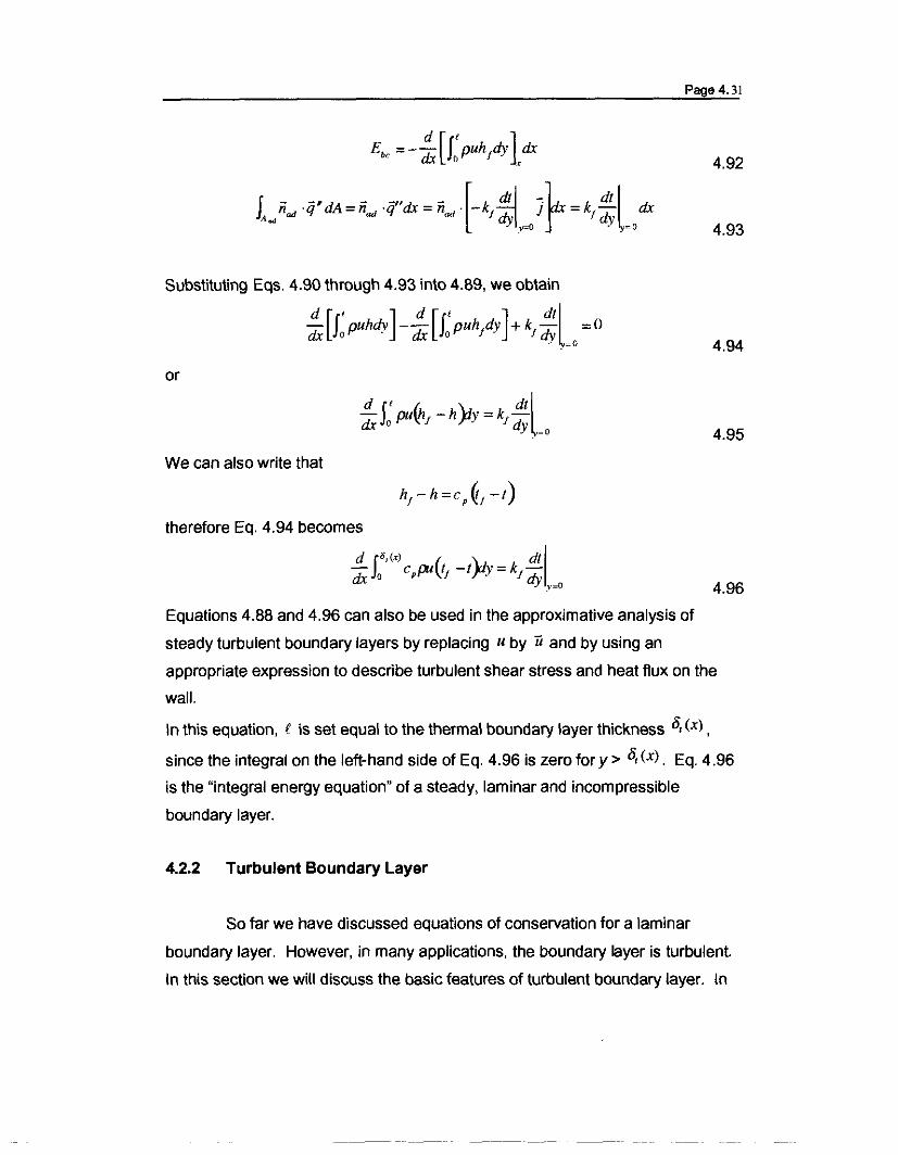
Substituting Eqs. 4.90 through 4.93 into 4.89. we obtain
~[J>UhdY]-~ [J:puhfdY] +kf:loo =0
or
We can also write that
therefore Eq. 4.94 becomes
d r5,(x) ( \"'. dlI
dx Jo CpfJU If -I?y =kfdYy=O
4.92
4.93
4.94
4.95
4.96
Equations 4.88 and 4.96 can also be used in the approximative analysis of
steady turbulent boundary layers by replacing U by u and by using an
appropriate expression to describe turbulent shear stress and heat flux on the
wall.
In this equation. £ is set equal to the thermal boundary layer thickness 8, (xl.
since the integral on the left-hand side of Eq. 4.96 is zero for y > 8, (xl. Eq. 4.96
is the "integral energy equation" of a steady, laminar and incompressible
boundary layer.
4.2.2 Turbulent Boundary Layer
So far we have discussed equations of conservation for a laminar
boundary layer. However. in many applications. the boundary layer is turbulent.
In this section we will discuss the basic features of turbulent boundary layer. In

Page 4.32
laminar flows, we have seen the heat and momentum are transferred across
streamlines only by molecular diffusion and the cross flow of properties is rather
small. In turbulent flow, the mixing mechanism, besides the molecular transport,
consists also macroscopic transport of fluid particles from adjacent layers
enhancing, therefore, the momentum and heat transport or in general, property
transport.
In order to understand the basic features of the turbulent boundary
layers and the governing equations we will assume that these equations for a
flow over a flat plate may be obtained from laminar boundary layer equations
(Eqs. 4.49, 4.50 and 4.58) by replacing U,V,t by;
u;;::.u+u'
v=v+v'1=1+1'
and taking the time average of these equations, We will further assume that the
velocity of the potential flow is constant. This implies that pressure also
constant. Under these conditions, the conservation equations for a turbulent
boundary layer are:
au av-+-=0ax ay
-at -at ()21 a - a-u-+v-=a---u'( --v't'ax ay ay' ax ay
4.97
4,98
4.99
Based on the experiments, in Eqs. 4.98 and 4.99 the terms :x (J2)can be
a t.7J) a_ a '(-\uv _ '( -vneglected relative to ay and ax u relative to iiy . Consequently, the
momentum and energy equations become:- - --au-aulaaua-
u-+v- = --f.l- --u'v'ax iiy p ay iiy ay

la a..,-;=--'r --u vpay , ay
-ai -ai a'i a-u-+v-=a---v'(ax ay ay' ay
=__I_~q;,_..iv't'PCp ay f ay
Page 4. 33
4.100
4.101
In the above equations the laminar expression for shear and heat flux
au'r, =Jl-ay
q"=-k atay
have been introduced to emphasize the origin of the terms involved. The shear
stress or, and heat flux q;' represent the flux of momentum and energy in the y
direction due to molecular scale activity.
a--,-, a,..-(-uv -vTo understand the significance of ay and ay terms, let us
consider a two dimensional flow in which the mean value of the velocity is
parallel to the x-direction as illustrated in Figure 4.11. Because of the turbulent
nature of the flow, at a given point, the instantaneous velocity of the fluid change
continuously in direction and magnitude as illustrated in Figure 4.12. The
instantaneous velocity components for the present flow are:

u.=u+u;~=u+~
y
u_ 1
S V'S
U'~2
o
Figure 4.11 Turbulent momentum exchange
)' ,
u, tv'
I
v; t:Jv[===;;t=:r'---JXt
Iu
Figure 4.12 Instantaneous turbulent velocities
u= u+u
v =v'
Page 4. 34
4.1UL
4.103

Page 4.35
As discussed in Section 4.1, an exchange of molecules between the
fluid layers on either side of the plane SS will produce a change in the x
direction momentum of the fluid because of the existence of the gradient in the
x-direction velocity. This momentum change of shearing force in the fluid which
is directed in the x-direction denoted by 7:, in Eq. 4.10. If turbulent velocity
fluctuations occur both in the x and y directions, which in the case under study,
the Y-direction fluctuations, v' transport fluid lumps which are large in
comparison to molecular transport across the surface SS' as illustrated in Fig.
4.11. For a unit area of SS, the instantaneous rate of mass transport across SS
is:
pv' 4.104
4.105
4.106
This mass transfer is accompanied by a transport of x-direction momentum.
Therefore, the instantaneous rate of transfer in the Y-direction of x -direction
momentum per unit area is given by:
-pv'(j,+ u')
where the minus sign, as will be shown later, takes into account the statistical
correlation between u'and v'. The time average of the x-momentum transfer
gives rise to a turbulent shear stress or Reynolds stress:
7:, = __1_J pv'(u+ u')17:Li 'fo 4'0
Breaking up Eq. 4.106 into two parts, the time average of the first is:
_1f (pv'}i~ir= 0~1'o A'ro 4.107
since Ii is a constant and the time average of (PV') is zero. Integrating the
second term of Eq. 4.106 gives:
7: = __1 f (pv')l d7: = -(pv')u', Ll7:o ". 4.108
or if P is constant:

f, = -PV'u'
Page 4.36
4.109
where v'u' is time average of the product of u'and v'. We must note that even
though 'if =;; =0, the average of the fluctuation product u'v' is not zero. To
understand the reason for introducing a minus sign in Eq. 4.105, let us consider
Fig. 4.13. From this figure we can see that the fluid lumps which travel upward
(v' > 0) arrive at a layer in the fluid in which the mean
y
....r-_u{""-y_+-'/)'--__~~-y+/
S ----I11'-_u.....:(:;..y:;..)---,.f- S ~/,/'-""::':'--:7"'5.f---t- y - i
x,u'-----------------------4.13 Mixing Ie ngth for momentum transfer
velocity u is larger than the layer from which they come. Assuming that the fluid
particles keep on the average their original velocity u during their migration, they
will tend to slow down other fluid particles after they have reached their
destination and thereby give rise to a negative component u'. Conversely, if
v'is negative, the observed value of u' at the new destination will be positive.
On the average, therefore, a positive v' is associated with a negative u', and
vice versa. The time average of u'v' is therefore not zero but a negative
quantity. The turbulent shear stress defined by Eq. 4.109 is thus positive and
has the same sign as the corresponding laminar shear stress f,. Based on the
above discussion Eq. 4.100 can be written as:- -
-au -av la( )uax+vay=pay f,+f,
f=f, +f,
4.110
4.111

4.112
Page 4. 37
is called total shear stress in turbulent flow.
To relate the turbulent momentum transport to the time-average velocity
gradient du Idy , Prandtl postulated that (Schlichting, 1979) the macroscopic
transport of momentum (also heat) in turbulent flow is similar to that of molecular
transport in laminar flow. To analyze molecular momentum transport (Section
4.1) we have introduced the concept of mean free path, or the average distance
a molecule travels between collisions. Prandtl used the same concept in the
description of turbulent momentum transport and defined a mixing length
(known as Prandtl mixing length), £ which shows the distance travelled by fluid
lumps in a direction normal to the mean flow while maintaining their identity and
physical properties. (e.g., momentum parallel to X-direction). Referring again to
Fig. 4.13, consider a fluid lump located at a distance £ (Prandtl mixing length)
above and below the surface 55. The velocity of the lump at y + £ would be:
i'.(y + £):!i(y)+ £ ~;
while at y- £:
4.113
If a fluid lump moves from layer y- £ to the layer y underthe influence of a
positive v' , its velocity in the new layer will be smaller than the velocity
prevailing there of an amount:
4.114
4.115
Similarly, a lump of fluid which arrives at y from the plane y + £ possesses a
velocity which exceeds that around it, the difference being:
- - auu{y +£)- u(y)= £ay

Page 4.38
Here v' < O. The velocity differences caused by the transverse motion can be
regarded as the turbulent velocity components at y. Examining Eqs. 4.114 and
4.115, it can be concluded that the u' fluctuation is in the same order of
,dumagnitude of <ry, i.e.,
U,,,,,,dU- dy
Substituting Eq. 4.116 into 4.109, we obtain
-dUT, =- fJ"" dY
or calling em =-v', , apparent kinematic viscosity,
dUT, =pem dy
4.116
4.117
4.118
The total shear stress is than given by (Eq. 4.111)
T=T, +T,(V+em~4.119
Prandtl has also argued that the v' fluctuation is of the same order as u'. em,
the apparent kinematic viscosity, is not a physical property of the fluid as J1 or v;it depends on the motion of the fluid and also on many parameters; the most
important is the Reynolds number of the flow. EO is also known to vary from point
to point in the flow field; it vanishes near the solid boundary where the
transverse fluctuations disappear. The ratio of e I V under certain circumstances
can go as high as 400 to 500. Under such cases, the viscous shear (i.e., V) is
negligible in comparison to the turbulent shear (/om) and may be omitted.
The transfer of heat in a turbulent flow can be modelled in a similar way
to that of the momentum transfer. Let us consider a two-dimensional time-mean
temperature distribution shown in Fig 4.14. The fluctuating velocity v'
continuously transports fluid particles and the energy stored in them across the
surface SS.

Page 4.39
y
y+/1 l(y) 1/,1 lq, (+)s s If1
y-l
X, t0'--------------------
4.14 Mixing length for energy transfer in turbulent flow
The instantaneous rate of energy transfer per unit have at any point in the y
direction is:
4.120
where t = t + t'. The time average of the turbulent heat transfer is given by:
1,'= +- i pv'~ + ()iruro ~ro 4.121
Carrying out the above integration we obtain:
q','= IX p v'I' 4.122
Substituting Eq. 4.122 into 4.101 we obtain:- -- at - at I a{ ~
u-+v-=---V(/+q;jat ay pCp ay
q" = 1,'+ ct:4.123
4.124
is called total heat flux in turbulent flow.
Using Prandtl's concept of mixing length we can write that:
( ~£dt- dy 4.125

Combining Eqs. 4.122 and 4.125 we obtain:
- -dt..."= fle v't' =-c pv'l'1, ~ p p dy
Page 4.40
4.126
Here, it is assumed that the transport mechanism of energy and momentum are
similar; therefore, the mixing lengths are equal. The product v'( is positive on
the average because a positive v' is accomplished by a positive (and vice
versa. The minus sign which appears in Eq. 4.17 is the consequence of the
conversion that the heat is taken to be positive in the direction of increasing y;
this also ensures that heat flows in the direction of decreasing temperature, thus
satisfies the second law of thermodynamics.
or
Representing by Eh = v'l Eq. 4.126 becomes
dtq;t pfJEh dy
The total heat transfer is then given by (4.124)
""k 'Ii!..!q =-~ +CpPEh1iy
dtq" = -cpp(a+E.)~
where a =k I (X p is the molecular diffusivity of heat. Eh is called the "eddy
diffusivity of heat" or eddy heat conductivity.
4.127
4.128
4.129
4.3 Forced Convection Over a Flat Plate
In the previous section we discussed velocity and thermal boundary
layers with extent of O(x) and ",(x), respectively. The velocity boundary layer is
characterized by the presence of velocity gradients, i.e., shear stresses whereas
the thermal boundary layer is characterized by temperature gradients, I.e., heat
transfer. From an engineering point of view we are mainly interested in
determining wall friction and heat transfer coefficients. In this section, we will
focus our attention on the determination of these coefficients for lamirar and

Page 4.41
turbulent flows. In order to reach rapidly the objectives, the integral momentum
and energy equations (Eqs. 4.88 and 4.96) will be used.
4.3.1 Laminar Boundary Layer
In laminar boundary layers, we discussed that fluid motion is very
orderly and it is possible to identify streamlines along which fluid particles move.
Fluid motion along a streamline has velocity components in x and y direction ( u
and V). The velocity component v normal to the wall, contributes significantly to
momentum and energy transfer through the boundary. Fluid motion normal to
the plate is brought about by the boundary layer growth in the x -direction
(Figure 4.8)
Consider a flat plate of constant temperature placed parallel to the
incident flow as shown in Fig. 4.15. Wewill assume that the potential velocity
u(x) and temperature II are constant. The constant potential velocity,
according Eq. 4.56 implies that longitudinal pressure gradient (in either the
potential region or on the boundary layer) is zero. It will also be assumed that
IF
Velocity boundarylayer
II,
U
•
•
yl0
1JC,lI,t
p=const.I, ""corul.
U=const.
Figure 4.15 Velocity & thermal boundary layers for laminar flow past a flat plate
4.130
Page 4.42
all physical properties are independent of temperature. In the following we will
determine the friction and heat transfer coefficient on the plate.
4.8.1.1 Velocity Boundary Layer - Friction Coefficient
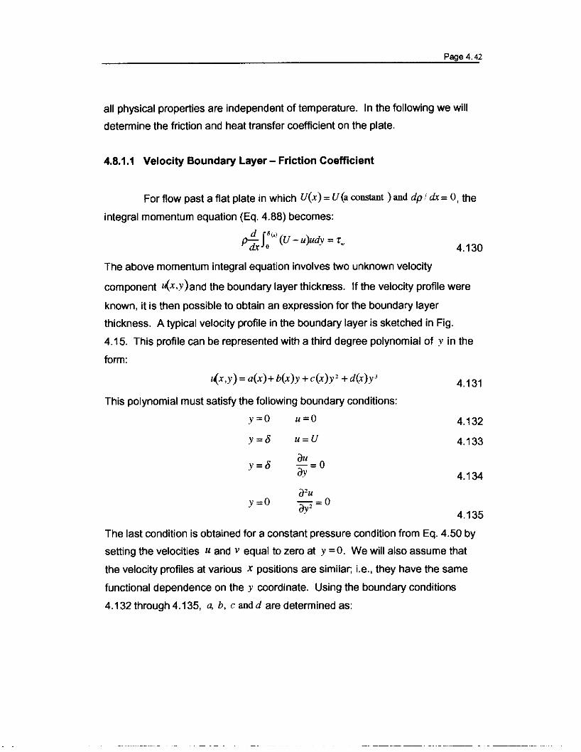
For flow past a flat plate in which U(x) =U (a constant) and dp Idx =0, the
integral momentum equation (Eq. 4.88) becomes:
d f'"'Pd;; 0 (U - u)udy = Tw
The above momentum integral equation involves two unknown velocity
component u(x,y)and the boundary layer thickness. If the velocity profile were
known, it is then possible to obtain an expression for the boundary layer
thickness. A typical velocity profile in the boundary layer is sketched in Fig.
4.15. This profile can be represented with a third degree polynomial of y in the
form:
u(x,y) =a(x)+ b(x)y +C(X)y2 + d(X)y3
This polynomial must satisfy the following boundary conditions:
y=o u=O
y=S u=U
y=S ou=ooy
4.131
4.132
4.133
4.134
y=O4.135
The last condition is obtained for a constant pressure condition from Eq. 4.50 by
setting the velocities U and v equal to zero at y =0. We will also assume that
the velocity profiles at various x positions are similar; i.e., they have the same
functional dependence on the y coordinate. Using the boundary conditions
4.132 through 4.135, a, b, C and d are determined as:

a=O3U
b=--28
c=OIU
d=--283
Page 4.43
4.136
and the following expression is obtained for the velocity profile:
~=~i-~(iJSUbstituting Eq. 4.137 into Eq. 4.130, knowing that:
~w =J{~) =~ Jl ~yoO
and carrying out the integration we obtain:
39 piP dO = ~ Jl U280 dx28
or
The integration of the above equation yields:
8 = 4.64.J'---~-u-1-x-+-c-ons-t.
4.137
4.138
4.139
4.140
4.141
4.142
Referring to Fig. 4.15 we see that at x =0, 8 =0, therefore the constant is zero
and the variation of the velocity boundary layer thickness is given by:
{jix8=4.64~p U
or
8 4.64 4.64
~= .JP~m =Re~24.143
R,= PUx
where Jl is the Reynolds number based on x, distance from the leading
edge.
The exact solution of the boundary layer equations (Eqs. 4.49 and 4.50)
yields:

Page 4.44
li 5.0
4.144
Therefore, Eq. 4.28 yields a value for li(x) 8% less than that of the exact
analysis. Since most of the experimental measurements are only accurate to
within 10%, the results of the approximate analysis are satisfactory in practice.
Combining Eqs. 4.138 and 4.143, we obtain for wall shear stress:
pU2Tw =0.323r,::=
.~Rex
Wall friction coefficient is defined as :
Tc~ =_\_w_
-pU'2
or with Eq. 4.145
c _0.646~-~
4.145
4.146
4.147
This is the local friction coefficient. The alerage friction coefficient is given by:
or with Eq. 4.147
c = 1.292x .JRex
4.3.1.2 Thermal Boundary Layer - Heat Transfer coefficient
4.148
4.149
Now, we will focus our attention to the thermal boundary layer and
determine the heat transfer coefficient. Consider again the flow on a flat plate
illustrated in Fig. 4.15. The temperature of the plate is kept at tw starting from
the leading edge and the temperature of the potential flow is tp and is constant.
Under the above conditions, a thermal boundary layer starts forming at the
leading edge of the plate. In order to determine the heat transfer coefficient, the

Page 4.45
thickness of the thermal boundary layer, 0, (x), should be known. To do so, we
will use the integral energy equation given by Eq. 4.96 and rewritten here for
convenience:
4.96
The above integral equation involves two unknowns: the temperature l(x,y) and
the thermal boundary layer thickness. If the temperature profile were known it
would then be possible to obtain an expression for the thermal boundary layer.
The velocity profile has already been determined and given by Eq. 4.137. A
typical temperature profile is given in Fig. 4.15. The profile, in a way similar to
that of the velocity profile, can be represented with a third degree polynomial of
y in the form:
I(X, y)= a(x) +b(x)y +c(x)y2 + d(x )y3
with boundary conditions:
y =0 t =t w
y=o, I = If
y=o,al-=0ay
a21y=O -=uay 2
4.150
4.151
4.152
4.153
4.154
The last condition is obtained from Eq. 4.58 by setting the velocities u and v
equal to zero at y = O. Under these conditions the temperature distributions is
given by:
Introducing a new temperature defined as:
0= I-Iw
Eqs. 4.96 and 4.155 can be written as:
4.155
4.156

Page 4.46
4.157
and
where 9. = II - I.
Substituting in Eq. 4.157 u and 9 by Eq. 4.137 and 4.158. we obtain:
9 U~t[l- ~z+.-!(z)3I~1_.!(I)3]dy =~a~• dx 0 2 0, 2 0, 2 0 2 0 2 0,
4.158
4.159
4.161
where a =kl / pc p
Defining ~ as the ratio of the thermal boundary layer thickness to the velocity
boundary layer thickness 0, /0. introducing this new parameter into Eq. 4.159,
performing the necessary algebraic manipulations and carrying out the
integration we obtain:
4.160
A simplification can be introduced at this point if we accept the fact that ~. the
ratio of boundary layer thickness, will be near 1 or better less than unity. We will
later see that this is true for Prandtl (Pr) numbers equal or greater than 1. This
situation is met for a great number of fluids. With the above assumption the
second term in the bracket in Eq. 4.160 can be neglected compared to the first
one and this equation becomes:
3 d 3 a 1__~2= _
20 dx 2~oU
or
4.162
Taking into account Eq. 4.140:
4.140

Page 4.47
and Eq. 4.142
t5 =4.64~E. xpU
and introducing them into Eq. 4.162, we obtain:
14l.{l(~3 +4X~2~) =113pa dx
4.142
4.163
4.165
1!:.- ~The ratio pa or a is a non-dimensional quantity frequently used in heat
transfer calculations; it is called the Prandtl number and has the following form:
Pr =H...!. =fJ. p: p =cpfJ.
pa p k j k j 4.164
With the above definition, Eq. 4.163 becomes;
(~3 +4X~2 d~) = 13..!..dx 14 Pr
or
4.166
Making a change of variable as :
Eq 3.166 is written as:
4dy 131y+-x-=--
3 dx 14 Pr 4.167
The homogeneous and particular solutions of the above equations are:
Homogeneous y=cx' wilh n=-3/4 4.168
131y=--
Particular 14 Pr 4.169
The general solution is then given by:
13 1 ~ly=--+Cx 4
14Pr 4.170
or

Page 4.48
4.171
1.; = 1.026 Pr 1/3
Since the plate is heated starting from the leading edge, the constant C must be
zero to avoid an indeterminate solution at the leading edge, therefore:
.;' =13 ....!.-14 Pr 4.172
or
4.173
In the forgoing analysis the assumption was made that';:51. This assumption,
according Eq. 4.173 is satisfactory for fluids having Prandtl numbers greater
than about 0.7. For a Prandtl number equal to 0.7, .; is about 0.91 which is
close enough to 1 and the approximations we made above is still acceptable.
Fortunately, most gases and liquids have Prandt numbers higher than 0.7.
Liquid metals constitute an exception: their Prandtl numbers are in the order of
0.01. Consequently the above analysis cannot be applied to liquid metals.
Returning now to our analysis, we know that the local heat transfer
coefficient was given by Eq. 4.2 which, for the present case, is written as:
where
(afJ) _~ fJ w _ ~ fJw
ay y;O - 2 0, - 2 c:SUbstituting Eq. 4.176 in Eq. 4.175, we obtain:
4.174
4.175
4.176

Page 4.49
4.177
4.179
4.178
This equation may be made non<limensional by multiplying both sides by x /k f:
hxx =0.332e.JPi.JpUxk f Jl
Combining the above equation with Eqs. 4.173 and 4.142 we obtain:
hx =0.332kf~~':
or NUx = 0.332;JP;~Rex 4.180
where NUx is the Nusselt number, defined as:
N hxxu.=kf 4.181
4.182
Eq. 4.180 express the local value of the heat transfer coefficient in terms of the
distance from the leading edge of the plate, potential flow velocity and physical
properties of the fluid. The average heat transfer coefficient can be obtained by
integrating over the length of the plate:
yhdxh f
o
L~ =2hX"L
hLNIL =-=2Nu_
-FL k x-L
f 4.183
or
- hLNu" =T=O.664Ret'Pr IB
f 4.184
where 4.185
The above analysis was based on the assumption that the fluid properties were
constant throughout the flow. If there is a substantial difference between the
wall and free stream temperature, the fluid properties should be evaluated at the
mean film temperature defined as:
--- -----------------
Page 4.50
Iw + If1=-m 2 4.186
It should be pointed out that the expressions given by Eqs. 4.180 and 4.185
apply to a constant temperature and when:
Pr ~O.7
Rex :s; 5x 10'
However, in many practical problems the surface heat flux is constant and the
objective is to find the distribution of the plate surface temperature for given fluid
flow conditions. For the constant heat flow case it was shown that the local
Nusselt number is given by:
Nu,. =O.453Re ~2 PrU34.187
4.3.2 Turbulent Boundary Layer
--~~-!II.ilrnlW!~!~
.I~«.~ ......... -...---~-..... ..-..---... ..... -.. .....eiliiiWdii!!X,II
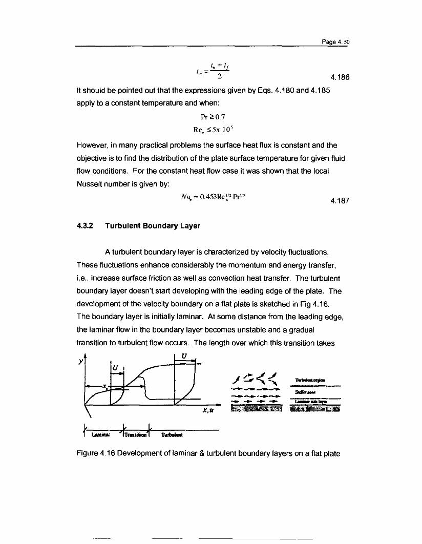
A turbulent boundary layer is ctBracterized by velocity fluctuations.
These fluctuations enhance considerably the momentum and energy transfer,
i.e., increase surface friction as well as convection heat transfer. The turbulent
boundary layer doesn't start developing with the leading edge of the plate. The
development of the velocity boundary on a flat plate is sketched in Fig 4.16.
The boundary layer is initially laminar. At some distance from the leading edge,
the laminar flow in the boundary layer becomes unstable and a gradual
transition to turbulent flow occurs. The length over which this transition takes
U
Figure 4.16 Development of laminar & turbulent boundary layers on a flat plate

Page 4.51
place is called" the transition zone". In the fully turbulent region, flow conditions
are characterized by a highly random, three-dimensional motion of fluid lumps.
The transition to turbulence is accompanied by an increase of the boundary
layer thickness, wall shear stress and the convection heat transfer coefficient.
In the turbulent boundary layer three different regions are observed
(Fig. 4.16):
1. A laminar sub-layer in which the diffusion dominates the property transport,
and the velocity and temperature profiles are nearly linear.
2. A buffer zone where the molecular diffusion and turbulent mixing are
comparable to property transport.
3. A turbulent zone in which the property transport is dominated by turbulent
mixing.
An important point in engineering applications is the estimation of the
transition location from laminar to turbulent boundary layer. This location,
denoted by x" is tied to a dimensionless grouping of parameters called the
Reynolds number:
Re = PUx
x f.J. 4.188
where the characteristic length x is the distance from the leading edge. The
critical Reynolds number is the value of Rex for which the transition to turbulent
boundary layer begins. For a flow over a flat plate the critical Reynolds number,
depending on the roughness of the surface and the turbulence level of the free
steam, varies between 10' to 3xlO'. It is usually recommended to use a value of
Rex =5xlO' for the transition point from laminar to turbulent flow. From Fig.
4.16, it is obvious that the transition zone for a certain length and a single point
of transition is an approximation. However, for most engineering applications
this approximation is acceptable. We should also emphasize that the flow in the
transition zone is quite complex and our knowledge of it is very limited.

u ()117_= .lU Ii
Page 4.52
4.3.2.1 Velocity Boundary Layer - Friction Coefficient
Analytical treatment of a turbulent boundary layer is very complex. This
is due to the fact that the apparent kinematic viscosity Em, as already pointed out
in Section 4.2.2, is not a properly of the fluid but depends on the motion of the
fluid itself, the boundary conditions, etc. Here, we will use a simple approach to
determine the thickness of the turbulent boundary layer.
The general characteristics of a turbulent boundary layer are similar to
those of a laminar boundary layer: the time-average flow velocity varies rapidly
from zero at the wall to the uniform value of the potential core. Due to the
transverse turbulent fluctuations, the velocity distribution is much more curved
near the wall than in a laminar flow case. However, the same distribution at the
outer edge of the turbulent layer is more uniform than that corresponding to a
laminar flow.
A number of experimental investigations have shown that the velocity in
a turbulent boundary layer may be adequately described by a one-seventh
power law:
4.189
where Ii is the boundary layer thickness and U is the time average ofturbulent
velocity. For the sake of simplicity the bar notation to show the time average is
dropped with understanding that all turbulent velocities referred to are time
averaged velocities. This power law represents well the experimental velocity
profiles for local Reynolds numbers in the range 5 x 10 5 < Re, < 107• Although
Eq. 4.189 describes well the velocity distribution in the turbulent layer, it is not
valid at the surface. This can be seen when we try to evaluate the shear stress
on the wall which has the following form:
4.190
.. _-_._- . - -------

Page 4.53
According to Eq. 4.189, the velocity gradient anywhere in the boundary is:
du 1 Udy 7 8'17 y617
4.191
4.192
4.130
This relation leads to an infinite value of the stress at the wall. This is not
physically possible. In our previous discussion, we have pointed out that the
turbulence dies out in the vicinity of the wall and the boundary layer behaves in
a laminar fashion. In this region, the velocity distribution is assumed to be
linear. Based on the above discussion, the velocity distribution in the turbulent
region, including the buffer zone, will follow one-seventh power law whereas in
the laminar sub-layer will be linear. This linear variation will be selected so that
the slope at y = 0 yields the wall stress obtained experimentally by Blasius
(1913) for turbulent flows on a smooth plate:
( )
114
'l'w =O.0228pU' ~O
where V is the kinematic viscosity. The velocity distribution in the laminar sub
layer will join to that in the fUlly turbulent region at a distance Os from the wall.
This distance is commonly called the thickness of the laminar sub-layer. The
resulting velocity profile is sketched in Fig. 4.17.
To determine the turbulent boundary layer thickness, we will employ Eq.
4.130, repeated here for convenience (u = constant, dp I dx = 0):
d f5 (X)IT;i;; 0 (U - u)udy ='l'w
Although the above equation is derived for a laminar flow, It may also be used
for a turbulent flow as long as the velocities used are time average velocities
and as long as wall shear term, 'l'w' is adequately represented for turbulent flow,
for example with Eq. 4.192 for a turbulent flow on a plate. For the purposes of
integral analysis, the momentum integral in Eq 4.130 can be evaluated by using
the power law given by Eq. 4.189. This is justified by the fact that the laminar
sub-layer is very thin. For the wall shear stress, the Blasius correlation given by
--- -- - --------- -

Page 4.54
yu
velocity bcu"""'Ylayer
x,vFigure 4.17 Velocity profiles in the turbulent zone and laminar sub-layer
Eq. 4.192 will be used. Consequently, the substitution of Eqs. 4.189 and 4.192
into 4.130 yields:
d ()1I7[ ()In] ( V )114pU2dxf: i 1- ~ =0.0228pU2 Uo
Integration of the above equation yields:
7 do o( V )11472 dx =0.022"1...uo
or
j )114OJ 14 do= 0.23\~ dx
This equation can be easily integrated to obtain:
j V)11S0= 0.37\ U X4'5 + constant
4.193
4.194
4.195
The constant may be evaluated for two physical situations:
1. The boundary layer is fully turbulent from the leading edge of the plate. In
this case boundary condition will be:
x =0 0=0 4.196
-------- - -------

Page 4.55
2. The bOlndary layer follows a laminar growth pattern up to R, =5 X 10' and a
turbulent growth thereafter. In this case the boundary condition will be:
o=o,atx=x =5x IO,Lcr pu 4.197
0, can be obtained from Eq. 4.144 repeated here for convenience:
o 4.64;= Rel/2
x 4.198
as:
4.200
{ )-1120, = 4.64x, \5 x 10'
4.199
For our application, we will retain the first option. Consequently, the constant in
Eq. 4.195 is zero and the thickness of the boundary layer is given by:
~ = 0.376 =0376Re-I/,
X (p~xr' x
This assumption is not true in practice. However, experiments show that the
predictions of Eq. 4.200 agree well IMth data. When Eq. 4.144 and 4.200 are
compared we observe that the thickness of the turbulent boundary layer
increases faster than that of laminar boundary layer. The equations for
boundary layer thickness (i.e., Eqs. 4.144 and 4.200) apply only to the regions
of fully laminar or fully turbulent boundary layers. As can be seen from Fig. 4.16
the transition from laminar flow to turbulent flow does not occur at a definite
point, but rather occurs over a finite length of the plate. The transition zone is a
region of highly irregular motion and the knowledge of the flow in this region is
quite limited. For most engineering applications, it is customary to assume that
the transition from laminar boundary to turbulent boundary occurs suddenly
when the local Rex number is equal to 5 x 10'. At the transition point the
thickness of the boundary layers will be different with the turbulent boundary
layer thicker than the laminar boundary layer; i.e., a discontinuity exists in the
thickness.

Page 4. 56
Let us now focus our attertion to the laminar sub-layer, illustrated in
Fig. 4.17 and determine its thickness, 6s , and the velocity of the fluid at the
juncture between the laminar sub-layer and the fUlly turbulent zone denoted by
Us.
Since the velocity varies linearly in the laminar sub-layer, the shear
stress in this layer is given by
du u1:=J1- =J1
dy y 4.201
Combining this expression with the wall shear stress correlation established by
Blasius for a turbulent boundary, we obtain for the variation of the velocity the
following expression:
u' ( )114u= 0.0228PJi P~6 y
when y =6s , u= us' the above expression becomes:
( )
314
§.. 1 J1 ~
6 0.0228 pU6 U
The velocity profile in the turbulent region was given by Eq. 4.189 which, for
y =6s and u =us, can be written as:
The combination of Eqs. 4.203 ans 4.204 yields:
4.202
4.203
4.204
4.205
6, the thickness of the turbulent boundary layer is given by Eq. 4.200, therefore
Eq. 4.205 becomes:
4.206
Combining Eqs. 4.204 and 4.206 we obtain:

0, 1948= Re~7
The wall shear stress can also be written as:
Using Eqs. 4.200, 4.206 and 4.207, the above equation becomes:
2 0.0296or. =pU Reo,
x
Page 4.57
4.207
4.208
4.209
4.210
1 7
Dividing both sides of this equation by '2 pU-and using the definition of the wall
friction coefficient, c... , given by Eq. 4.146, we obtain:
C _~_0.0592~ - 1 - Re02
-pU' ,2
This is the local wall friction coefficient.
4.3.2.2 Heat Transfer in the Turbulent Boundary Layer
The concepts regarding turbulent boundary layers discussed in
Sections 4.2.2 and 4.3.2.1 will now be employed for the analysis of heat transfer
as flat plates in turbulent flow. We will first discuss the Reynolds analogy for
momentum and heat transfer. Subsequently we will discuss a more refined
analogy introduced by Prandtl.
Reynolds Analogy for Laminar boundary layer
In a two-dimensional laminar boundary layer, the shear stress at a
plane located at y is given by:
duor =J.l
dy
The heat flux across the some plane is:
"--k dtq - f dy
4.211
4.212

Dividing Eqs. 4.211 and 4.212 side by side, we obtain
q" kf dtT=-ji du
This expression can also be written as:
1:..=_!Lc dl'l" Jlc p P du
Page 4.58
4.213
4.214
jlcp / k p is the Prandtl number. Reynolds assumes that Pr =j, therefore Eq.
4.214 becomes:
q" dl-:-c
'l" p du 4.215
Assuming that q" / 'l" ratio is constant and equal to the same ratio on the wall,
i.e.,
q" q~-=-
'l" 'l"w 4.216
Eq. 4.215 can be easily integrated from the wall conditions I = I., u = c , to the
potential flow conditions I =If' u =U ,
on
" uqwJ du=-c J'I dl". 0 P I'w •
d' 'l" c~-~I -I - Uw f
4.217
4.218
The left hand side of Eq. 4.218 is nothing else but convection heat transfer, h.
Therefore we write:
'fwc p
h=lj
Using the definition of wall friction coefficient
'l"wc.. =-j--
-pU'2
Eq. 4.219 becomesj
h=-pUc c2 P f
4.219
4.146
4.220

Page 4.59
Multiplying both sides of the above expressing x, knowing that for
Pr =1, cp =k! / fJ., and using the definition of local Reynolds number
Re = PUx
x fJ.
and local Nusselt number:
Eq. 4.147 is written as:
1Nu =-c Re
x 2 '1' x
This is the dimensionless statement of Reynolds' analogy for laminar flow.
Observe that heat transfer coefficient is related to the wall friction factor.
4.221
In Section 4.3.1.1 it was shown that for a laminar flow on a flat plate, the
wall friction coefficient was given by (Eq. 4.147)
0.646c =--.. Re~2 4.147
For this case Reynolds analogy (Eq. 4.221) gives:
Nu = 0.332Re1l2x x 4.222
The result obtained from the integral momentum and energy analysis was (Eq.
4.180)
Nu =0.332Rel12 Prwx x 4.180
For Pr = I, this result is the same as the one obtained by Reynolds' analogy.
Therefore, there is an agreement between Eqs. 4.180 and 4.222. It appears
that the effect of the Prandtl number differing from unity can be expressed by a
factor equal to Pr"3. The latter fact is sometimes applied in other cases when
exact solution to the thenmal boundary layer cannot be obtained, and
experimental skim friction measurements are used to predict heat transfer
coefficients.
Reynolds' analogy for turbulent boundary layer
----- --------

4.119
Page 4.60
In Section 4.2.2, we have seen that the total shear stress and heat flux
in a turbulent boundary layer were given by Eqs. 4.119 and 4.129, respectively.
These equations are repeated here for convenience:
7:=7:, +7:,(V+em~
4.129
where V: is the kinematic viscosity related to molecular momentum exchange
(molecular diffusivity of momentum)
em: is the apparent kinematic viscosity related to turbulent momentum
exchange (eddy diffusivity of momentum)
a : is the molecular diffusivity of heat
eH : is the eddy diffusivity of heat
Reynolds assumed that the entire flow in the boundary layer was turbulent. This
means that he neglected the existence of the viscous sub-layer and the buffer
zone. Under these conditions the molecular diffusivities of momentum (V) and
heat ( a) can be neglected in comparison with turbulent diffusivities (em and eH ),
i.e.,
V «em and a« e4
Moreover, Reynolds assumed that:
Em=eH=e
Under these conditions, Eqs. 4.119 and 4.129 become:
du7:=7:, =pe
dy
dtq" =q"=-pc e-
, P dy
Dividing Eqs. 4.225 and 4.224 side by side, we obtain
t/.' dt...1..=-c 7:, P du
4.223
4.224
4.225
Comparing Eq. 4.226 with Eq. 4.215, we observe that these equations are
similar provided that in laminar boundary layer the Prandtl number is equal to 1.

Page 4. 61
Comparing Eq. 4.226 with Eq. 4.215. we observe that these equations are
similar provided that in laminar boundary layer the Prandtl number is equal to 1.
Prandtl's Modification to Reynolds' Analogy
Prandtl assumed that the turbulent boundary layer consisted of two
layers:
1. A viscous layer where the molecular diffusivities are dominant. that is:
V» Em and a» EH 4.227
2. A turbulent zone where the turbulent diffusivities are dominant, that is:
4.228
He also assumed that Em = EH = E. This approach implies that the Prandtl
number is not necessarily equal to 1.
The variation of velocity and temperature in this two-region boundary
layer is illustrated in Fig. 4.18. In the laminar sub-layer. the velocity and the
temperature vary linearly: from zero to Us for velocity and from Iw to Is. for
temperature. In the turbulent region the variation of the velocity. as discussed in
Section 4.3.2.1 is given by one-seventh power law (Eq. 4.189) and varies from
Us to U • \elocity of the potential flow. whereas the temperature varies from
Is to Ip • temperature of the potential flow.
Applying Eq. 4.213 to the laminar sub-layer we write:
q" kf-du=--dlT Jl. 4.229
Integrating this equation between 0 and Us and between Iwand lSI assuming that
" "'L qwT ratio is consta nt and equal to Tw we obtain:
or
" u k t'b.J 'du= _....Lf.. dlf w 0 J.1 t '"
-- - - - - -- - --
4.230

Page 4.62
y. .u
............... -.- .......~-----1Hr---t'
Tempenmre
Velocity
U.
X,u,t
Figure 4.18 Turbulent boundary layer consisting of two layers: Prandtl approach
if..'="t kf 2.(1 _ I )\Ii \Ii II Us \:. ~
,. 4.231
Applying now Eq. 4.226 to the turbulent region of the boundary layer we write:
cf.'....!..du=-c dl"t, p 4.232
Integrating this equation between 't and U , and between I. and If. (see Fig.
4.18) and assuming again q;'I"t, ratio is constant and equal to q~ / "t., we obtain:
" vq'f du=-c f'l dl'fw Us P t.rj
or
"fVq", du =-c f'l dl1'w Us P ''1
The elimination of I. , between Equ. 4.231 and 4.234 yields
a' (IlU. u-u)I. - If =.:ll< =-"- + .:::....-="t. kf c p
Knowing that:
4.233
4.234
4.235

Page 4.63
4.1
Eq. 4.235 is written as:
1
fwC p
h= U, u1+=(Pr-I)
U
4.236
4.237
The above equation is the statement of PrandU's modification of Reynolds'
analogy and may be written in a dimensionless form by multiplying both sides
x IkI and by rearranging the numerator:
.!:.~lIce Uxp
2!.pU2 kl 11Nu =----'2~::- _
x u1+=U (Pr-I)
4.238
Recognizing that:
Eq 4.238 becomes:
1-c ·Pr·Re2 ~Nu,,= ....-~-u
1+ -'-'(Pr-l)U 4.239
u,For a turbulent flow c~ and U are given with Eqs. 4.206 and 4.210, repeated
here for convenience:
u, 2.12-=--U ReO.!
4.206
C~0.0592Re~·2 4.207

Substituting these relationships into Eq. 4.239, we obtain:
00292 Re08 PrN -' •u, - 1+ 2.12 Re;"I(Pr_l)
Page 4.64
4.240
Nu, =0.0292 Reo, Pr"
This relation is found to give adequate results for turbulent heat transfer
coefficients in spite of many simplifications. The fluid properties in Eq. 4.208
should be evaluated at the mean temperature and the Prandtl number should
not be too different from unity. The major difficulty of Eq. 4.240 is its integration
to obtain the average Nusselt number. It is observed that for Pr numbers not
different from unity, which is the case for many gases and liquids, the
denominator of Eq. 4.240 is nearly constant. Therefore, for such cases it is
recommended that following expression be used in the estimation of the heat
transfer coefficient:
4.241
Again the mean film temperature (Eq 4.186) should be used for all properties.
Eq. 4.241 can be integrated along the plate to obtain an average Nusselt
number. For a plate length L, this average is given by
Ii, ="!'[0.0292 PrI/3(PU)O" k IL_I-dx]L J1 jOX02
or
4.242
This latter relation assumes that the boundary layer is turbulent starting from the
leading edge of the plate. As discussed in Section 4.3.2 and illustrated in Fig.
4.16, starting from the leading edge over certain portion of the plate the
boundary layer is laminar. The transition to turbulent flow occurs at a distance
X,. This point is specified by a critical Reynolds number; usually a value of
5 x 10' is used. Under these conditions, a better average film coefficient and
average Nusselt number would be given by the combination of Eqs. 4.180 and
4.241:

Page 4.65
ii, =1. [0.332 PrI13 k(PU)1/2 rx, _1 dx
L f Jl Jo X ll2
-10.0292 Prl/3 k (pU)O"fL _1_ dx ]f 11 x ... X O.2
4.243
In the above averaging, it is assumed that the laminar to turbulent
transition occurs instantaneously. The following expression is obtained for the
average Nusselt number:
NUr. =0.036 PrIl3[Re~'_ Re~:+ 18.44 Re~,'] 4.244
where Re"is the critical Reynolds number. If Re,,=500,OOO, the above relation
becomes:
4.245
4.4 Forced Convection in Ducts
Heating and cooling of fluid flowing inside a duct constitutes one of the
most frequently encountered engineering problems. The design and analysis of
heat exchanges, boilers, economizers, super heater and nuclear reactors
depend largely on the heat exchange process between the fluid and the wall of
the tubes.
The flow inside a duct can be laminar or turbulent. The turbulent flow
inside ducts is the most widely encountered type in various industrial
applications. Laminar flow inside ducts is mainly encountered in compact heat
exchanges, in the heating and cooling of heavy fluids such as oils, etc.
When a fluid with uniform velocity enters a straight pipe a velocity
boundary layer (also a thermal boundary layer, if the tube is heated) starts
developing along the surface of the pipe as illustrated in Fig. 4.19.
--- -_._---

Page 4.66
Poecntial COle CoqJletely developedBouw.ialy layer
/ Dow
'""~ """ I ............. "- -......"' ""
······~·4···\.•. .......... .........................'.' ........J
/J ./'
../ ./ ~
--------
Enlrance length
4.19 Flow in the entrance region of a pipe
Near the entrance of the pipe, the boundary layer develops in a way similar to
that on a flat plate. Because of the presence of an opposite wall on which a
boundary layer also develops, at a given point along the tube, both boundary
layers will touch each other and fill the entire tube. The length of the tube m.er
which the viscous layers have grown together and filled the tube cross section is
called the starting or entrance length. The flow beyond this region is termed
"fully developed flow". In the entrance region the flow consist of a potential core
region near the centre of the tube where the velocity is uniform and a boundary
region near the wall of the tube where the velocity varies from the potential core
value to zero at the wall. As we proceed along the pipe in the entrance region,
the portion of the tube occupied by the boundary layer, where the flow velocity
varies, increases and the position occupied by the potential core decreases.
Consequently, in order to satisfy the principle of mass conservation, i.e., a
constant average velocity, the velocity of the potential core shouts increase.
This increase is illustrated in Fig. 4.19.
The transition from laminar to turbulent flow is likely to occur in the
entrance length. If the boundary layer is laminar until it fills the tube, the flow in
the fully developed region will be laminar with a parabolic velocity profile.
However, if the transition from laminar to turbulent flow occurs in the entrance

Page 4.67
region, the flow in the fully developed region will be turbulent with somewhat
blunter velocity profile as illustrated in Fig. 4.20. In a tube, the Reynolds number
based on the diameter:
Re = PUmDD J1
is used as a criterion for the transition from laminar to turbulent flow.
"R ............L .. u_.... ..... ~...... , ..... , .. _,.
'"
/ U.. 1/I '"
Figure 4.20 Velocity profile in turbulent pipe flow
4.246
4.248
Here D is the pipe diameter and Um is the average velocity of the flow in the
pipe. for:
ReD> 2300
the flow is usually observed to be turbulent. This value should not be treated as
a precise value. since a range of Reynolds numbers for transition has been
experimentally observed depending on the pipe roughness and the smoothness
of the flow. The generally accepted range for transition is:
2000 < Re D< 4000 4.247
For laminar flow, the length of the entrance region maybe obtained from an
expression of the flow (Langhaar. 1942)
~ =0.0575 ReD
---------------_._...

Page 4.68
There is no satisfactory expression for the entry length in turbulent flow, it is
known that this length is practically independent of Reynolds number and, as a
first approximation it can be assured that (Kay and Crawford, 1980.)
IOS Ls S60D 4.249
Usually it is assumed that the turbulent flow is fUlly developed for Ls /D > 10.
4.4.1 Laminar Flow
In this section, the velocity distribution, frictional pressure loses and the
convection heat transfer coefficient will be discussed for the fully developed
region. The discussion of the entrance region is beyond the scope of this
lecture.
4.4.1.1 Velocity Distribution and Friction Factor in Laminar Flow
The form of the velocity can be easily determined for a steady state
laminar flow of an incompressible, constant property flow in the fully developed
region of a circular tube. In the fully developed region, velocity profile doe not
change along the tube. It depends only on the radius, i.e., U= u(r).
To proceed with the analysis, let us select a fix control volume of radius
r and length dx sketched in Fig. 4.21. The application of the macroscopic
momentum balance (Eq. 2.22) to the above control volume yields (see Eq. 4.63)
-t;,· pVvdA -Lii. /idA+L;, ·adA=o4.63
Multiplying this equation by r and knowing that the velocity profile does not
change in the x-direction (ie·.rl ii· pvVdA =0), we obtain:
-7· t ii· pldA +7 {n.adA =04.250

Page 4.69
I,dx
Rr-_ -
p+fIpdx Xdx
,I
4.251
Figure 4.21 Control volume in a laminar, fully developed flow in a
circular tube
which is simply a balance equation between of the forces acting on the control
volume. Le., balance between shear and pressure forces in the flow. The
pressure and viscous stress terms in Eq 4.250 can be written as:
-f-= (dn'L dp-i· A n' pl' dA=-p/fr' + Px +"d;;dxrr2 =rcr'- dx dx
-7- f ii· ~dA =-21!'rdxTA '
SUbstituting Eqs. 4.251 and 4.252 into 4.250 we obtain:
r dp--=-T2 dx '
We know that:
duT, =-/1 dy
and this equation with y = R- r (or dy = -dr) becomes:
duT, = -/1 dr
Substitution of Eq. 4.254 into Eq. 4.253 yields:
du= ~(:}dr
Since the axial pressure gradient is independent of r, Eq. 4.255 may be
integrated to obtain:
4.252
4.253
4.254
4.255

u= 4~(:)r'+C
The constant C can be easily determined by setting:
r=R u=OTherefore, the constant becomes:
C =__I (1E)R24/1 dx
It follows that the velocity profile oHhe fully developed flow is given by:
u=_1 (dP)R'(I_-'c)=U (I_-'c")4/1 dx R' = R'
Page 4. 70
4.256
4.257
4.258
4.259
Hence the fully developed profile is parabolic. Note that the pressure gradient
must always be negative.
The average velocity is given by:
_J: 2JrrpudrUm - JrR2
Substituting u in the above equation by Eq. 4.259 and carrying out the
integration, we obtain:
Substituting this result into Eq. 4.259, the velocity profile is then
l(r)=2Um(l- ~:)
U m can be calculated from the knowledge of the volume flow rate:
QU =
m A
4.260
4.261
4.262
4.263
where Q is the volume flow rate in m3/ S and A is the flow section in 11f. Eq.
4.262 can be used to determine frictional pressure gradient.

Page 4. 71
Eq. 4.253 can also be written for a control volume bounded by the tube
wall and two planes perpendicular to the axis and a distance dx apart as:
B.EE =-T2 dx R 4.264
or as
where D is the diameter of the tube. TR is given by:
T =_~dU)R dr
r~R
1Dividing both sides of Eq. 4.265 by 2pU~ and calling:
!-~- 1-pU'2 m
we write
4.265
4.266
4.268
where ! is the friction factor. Since the velocity distribution is known TR can be
easily evaluated from Eq. 4.266 as:
8 UmT = fI-
R r- D 4.269
The substitution of Eq. 4.269 into Eq. 4.267
64Jl 64!=-=
pUmD ReD
where
pipe.
Re (= pUmD
)D Jl is the Reynolds number based on the diameter of the
4.270
Equation 2.268 in conjunction with Eq. 2.270 allows us to evaluate the
frictional gradient component of the total pressure gradient in a laminar flow.
The pressure drop in a tube of length L is obtained by integrating Eq. 2.268:
IP, JL 1 U 2 1 L
/',p=- dp= f-~dx=f-pU2-II 0 2 D 2 mD
4.4.1.2 Bulk Temperature
Page 4. 72
4.271
For flow over a flat plate, the convection heat transfer coefficient was
defined as:
4.272
4.273
where If is the temperature of the potential stream. However, in a tube flow
there is no easily discemible free-stream condition. Even the centerline
temperature (Ie) cannot be easily expressed in terms of inlet flow parameter and
wall heat flux. Consequently, for fully developed pipe flow it is customary to
define a so-called "bulk temperature" in the following form:
iRpc ltil.11Tdr
t _ 0 P
b- JR puc 21fTdro p
For incompressible flow with constart cp, this definition is written as:
rpCptu2rrrdrI, ==------'---
mCp
4.274
The numerator of Eq. 4.273 or 4.274 represents the total energy flow through
the tube, and the denominator represents the product of mass flow and specific
heat integrated over the flow area. The bulk temperature is thus representative
of the total energy of the flow at a particular location along the tube.
Consequently, as can be seen from Eq. 4.274, the multiplication of the bulk
temperature with the mass flow rate and the specific heat given the rate at which
thermal energy is transported with the fluid as it moves along the tube.
With the above definition of the "bulk temperature", the local heat
transfer coefficient is than defined as:

q"h
~w -I,)
where lw is the pipe wall temperature.
Page 4, 73
4.275
In practice, in a heated tube an energy balance may be used to
determine the bulk temperature and its variation along the tube. Consider the
tube flow seen in Fig. 4.22. The flow rate of the fluid and its inlet temperature
(or enthalpy) to the tube are m, respectively. Convection heat transfer occurs at
the inner surface.
------1--1-q-;-+-----
.......................-.- - , , , .
I,
t---dx---tIxo x
h
x+dxh+ dh dx
dx
Figure 4.22 Control volumes for integral flow in a tube
Usually, fluid kinetic and potential energies, viscous dissipation and axial heat
conduction are negligible. Steady state conditions prevail. Under these
conditions the variation of the bulk temperature along the tube will be
determined for "constant surface heat flux" and for "constant surface
temperature".
1. Constant surface heat flux
Representing by q~ constant wall heat flux and applying the energy
conservation equation (Eq. 4.64) to the control volume limited by the tube wall

Page 4.74
and by two planes perpendicular to the axis and a distance dx apart (Fig. 4.22),
we can write:
4.276
or
Integration of this equation between the inlet of the tube and a given axial
position (x) yields:
h(x)-h, =~ q".l:m
Enthalpy difference h- h, can be written in terms of temperature as:
h(x)-h, =~ p[lb(X)- dCombining Eqs. 4.278 and 4.279, we obtain the variation of the bulk
temperature along the tube as:
1fD •I,(x) =1, +-.-qwx
m
2. Constant surface temperature
Results for the axial distribution of the mean temperature are quite
different when the temperature of wall is maintained at a constant value Iw •
Under this condition the local wall heat flux is given by:
q~(x)= holl. -lb(X)]
4.277
4.278
4.279
4.280
4.281
where h, is the convection heat transfer coefficient. Substituting Eq. 4.281 into
Eq. 4.277 and knowing that:
we obtain:
4.282
dl
Iw-I,(x)
Integration of this equation yields:
1fD h, dxt+--, mCp
4.283

or
rrD r'InUw -I,(X)) =-:--C Jo h,dx+ Cm p
Page 4.75
4.284
Iw -I.(X) = expC'· exp( :)0'h,dx )=c'exp(:):hjJx ) 4.285
The constant C can be determined using the boundary condition.
4.286
4.290
4.291
as
C =Iw - lbi 4.287
The variation of the bulk temperature along the tube is then given by:
Iw -I. (x) exp( ~ f: hjJX) 4.288tw -fbi mep
Defining the average value of h, from tube inlet to x as
- ii'h, =- h dxx 0 ' 4.289
Eq. 4.288 is written as:
Iw -I. (x) (rrDX h- )exp --tw-f
Nme
pc
This equation tells us that the temperature difference Iw - I. (x) decays
exponentially with the distance along the tube axis. The temperature at the exit
of the tube is obtained by setting x =L in Eqs. 4.288 and 4.289 as:
-"Iw'-----"I''''-(x~) (1tDL h- )- -exp -.- ,L
Iw -Ibi mCp
where ha. is the average value of he for the entire tube.
Eq. 4.288 allows us to determine the bulk temperature I.(x) at a given
axial position. If he can be taken as constant along the tube, the determination
of t. (x) is straightforward. If not, iterations are required to determine the value

Page 4.76
of tb(x) is straightforward. If not, iterations are required to determine the value
of the bulk temperature. The bulk temperature concept introduced in this
section is applicable to both laminar and turbulent flows in tubes.
4.4.1.3 Heat Transfer in Fully Developed Laminar Flow
Although the analysis of the velocity distribution for fully laminar pipe
flow is relatively simple, Eq. 4.262, the analysis of temperature distribution and
consequently film coefficient is complex.
In a circular tube with uniform wall heat flux and fully developed laminar
flow condition, it is analytically found that the Nusselt number is constant,
independent of ReD. Pr and axial location: (Ozirik, 1985), i.e.,
NIL = hoD =4364.." k . 4.292
In this analytical derivation, it is assumed that the velocity distribution in the tube
is given by Eq. 4.262 which is true for isothermal flows. For constant surface
temperature conditions, it is also found that the Nusselt number is constant:
hDNUo =--"-k =3.66
4.293
Again, Eq. 4.262 is used for velocity distribution in this analytical analysis.
The use of a velocity distribution corresponding to isothermal flow
condition is only valid for small temperature differences between the fluid and
the tube wall. For large temperature differences, the fluid velocity distribution
will be influenced by these differences as indicated in Fig. 4.23. Curve b shows
the fully developed parabolic distribution that would result for isothermal or very
small temperature difference flow. When the heating is significant, the viscosity
is lowest near the wall; as a result, the velocity increase (curve a)

Page 4. 77
+-#-.~-~--+'<\-+- U.
R
Figure 4.23 Influence of large temperature differences on velocity
distributions in a tube
is faster than the isothermal case. (curve b). For the cooling, the reverse
occurs as indicated by curve c of Fig. 4.23: the viscosity is highest near the wall
and the velocity increase is slower than the isothermal case. Consequently,
although Eqs. 4.292 and 4.293 are enticing by their simplicity, for the above
given reasons, they should not yield accurate convection heat transfer
coefficient for laminar flows. Moreover, Eqs. 4.292 and 4.293 are only
applicable to fully developed laminar flow conditions. As we discussed in
laminar flows, the entrance region is quite substantial. In fact, in short tubes this
region can occupy the entire length of the tube.
In parallel to the analytical studies, empirical relations have been
developed to predict convection heat transfer for laminar flows in the entrance
region of a circular tube. Hauseri(1943) developed the following empirical
relation for laminar flow in a circular tube at constant wall temperature:
--- ._.- ----

- h,D _....:O....:.0668--'-'-::'->(D=--..;/L:;<).::..cRe:..J,p""Pr-,="NUD =- =3.66+kI 1+O.04[(D IL)Re D PrJ"
Page 4.78
4.294
where NUD is the average Nusselt number. The above empirical relation
approaches to the limiting value Nun = 3.66 (Eq. 4.293) as the pipe lergth
becomes very great compared with the diameter. In this relation the fluid
properties are evaluated at the bulk temperature. Eq. 4.294 is recommended
for:
ReD Pr < 100LID
Sieder and Tale(1936) gave the following more convenient empirical correlation:
( )113( )0.14
NUD =1.86Re~3PrV3 ~ 1t4.295
The fluid properties are to be evaluated at the bulk fluid temperature except for
the quantity Jiw, dynamic viscosity, which is evaluated at the wall temperature.
The term (P, /Jiw )' 14 is included to account for the fact that the boundary layer at
the pipe surface is strongly influenced by the temperature dependence of the
roo )0.14
viscosity. This is particularly true for oils. The term VL, / Jiw applies to both
heating and cooling cases. The effect of starting length is included in the term
(D/ L)113The range of applicability of Eq. 4.295:
0.48 < Pr < 16.700
Jl.0.0044< - < 9.75J1w
(Re Pr JlI3( )0,14
P &. ~2LID J1w
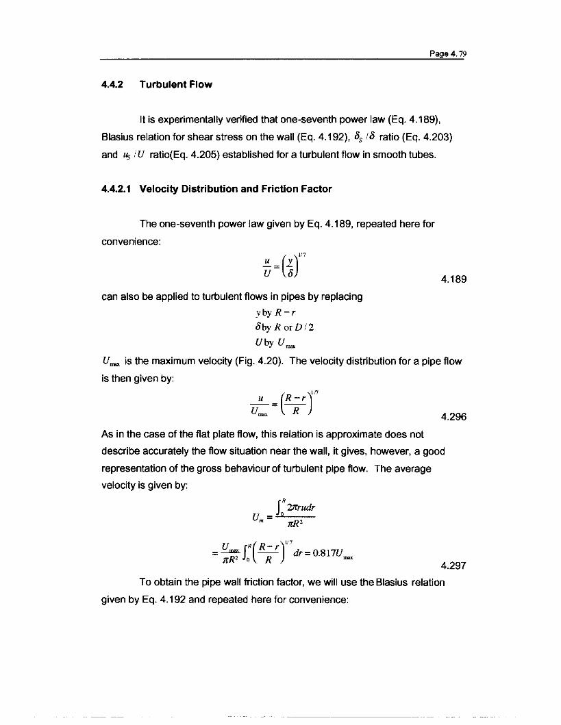
Page 4.79
4.4.2 Turbulent Flow
It is experimentally verified that one-seventh power law (Eq. 4.189),
Blasius relation for shear stress on the wall (Eq. 4.192), Os I°ratio (Eq. 4.203)
and Us IU ratlo(Eq. 4.205) established for a turbulent flow in smooth tubes.
4.4.2.1 Velocity Distribution and Friction Factor
The one-seventh power law given by Eq. 4.189, repeated here for
convenience:
4.189
can also be applied to turbulent flows in pipes by replacing
yby R - r
oby R or D /2
Uby U=
U""" is the maximum velocity (Fig. 4.20). The velocity distribution for a pipe flow
is then given by:
U: =(R;rf4.296
As in the case of the flat plate flow, this relation is approximate does not
describe accurately the flow situation near the wall, it gives, however, a good
representation of the gross behaviour of turbulent pipe flow. The average
velocity is given by:
_J: 21rrudrUm - TrR'
U R(R )117=~ f ---.::..!. dr = O.817U
nR' 0 R =4.297
To obtain the pipe wall friction factor, we will use the Blasius relation
given by Eq. 4.192 and repeated here for convenience:

(r )114
Tw =O.0228pU' UO
Replacing,
Tw by T.
oby D/2
Uby U =...!!...= 0.817
we obtain:
T = 0.089pU' (~)Jl4R m UmD
or using the definition of the friction factor given by Eq. 4.267
!_~_ 0.312 _ 0.312- 1 - (U D)Jl4 - Rel14
-pU',;:"m;;;;". D2 m V
Page 4. 80
4.192
4.298
4.299
The above relation fits the experimental data well for:
104 < ReD <Sx 104
If the constant 0.312 is replaced by 0.316, the upper limit can be extended to
10'. For higher ReD numbers the following relation can be used:
Prandtl Equation
-+:=2.0Iog (Re.JJ}-0.8 3000 <ReD <3.4x 10⁶
'J! 4.300
von Karman Equation
1,.-; =2.0 log (D / E)+ 1.74'J!
o 1--;:-r: >0.01E Re-,J! 4.301
4.268
Several friction factor correlations are available in the literature.
For turbulent flows, the frictional pressure gradient is given by the came
expression obtained for laminar flows (Eq. 4.268) repeated here:
dp 1 1- dx=!2PU~D
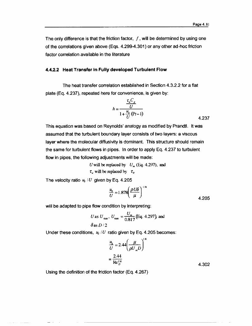
h
Page 4.81
The only difference is that the friction factor, f, will be determined by using one
of the correlations given above (Eqs. 4.299-4.301) or any other ad-hoc friction
factor correlation available in the literature
4.4.2.2 Heat Transfer in Fully developed Turbulent Flow
The heat transfer correlation established in Section 4.3.2.2 for a flat
plate (Eq. 4.237), repeated here for convenience, is given by:
TwC p
V
1+~(Pr-I)V 4.237
4.205
This equation was based on Reynolds' analogy as modified by Prandtl. It was
assumed that the turbulent boundary layer consists of two layers: a viscous
layer where the molecular diffusivity is dominant. This structure should remain
the same for turbulent flows in pipes. In order to apply Eq. 4.237 to turbulent
flow in pipes, the following adjustments will be made:
V will be replaced by Vm (Eq. 4.297), and
Tw will be replaced by TR
The velocity ratio Us f V given by Eq. 4.205
~ =1.87{p~or~
will be adapted to pipe flow condition by interpreting:
VVas V =' V= =O.8~7(Eq. 4.297) and
oas D /2
Under these conditions, Us /V ratio given by Eq. 4.205 becomes:
~=244(:mDr2.44Re"8
D
Using the definition of the friction factor (Eq. 4.267)
4.302

I-~- 1-pU2
2 m
the wall shear stress orR can be written as:
or = I PU2R 8 m
We will assume that 1 is given by:
1 =°.316Re°·25
Page 4.82
4.267
4.303
4.304
Replacing in Eq. 4.287, Uby U m, using Eqs. 4.302, 4.303 and 4.304, and
introducing the Nusselt number (Nu= hp / k!) and diameter Reynolds number
(ReD =PUmD/ jl), we obtain:
4.305
Experiments show that the relation works reasonably well in spite of the
simplifying assumptions that have been made in its derivation. It is usually
suggested (Hoffman, 1938) that the constant 2.44 in Eq 4.305 be replaced by:
1.5Pr-!16
ConsequenUy, Eq. 4.305 becomes:
_ 0.0396 ReI!' PrNu" -1+1.5Pr-l'ReL!"(Pr-I)
4.306
4.307
Both of these relations are based on the determination of the fluid properties at
the bulk fluid temperature. Eqs. 4.305 and 4.307 give good results for fluids with
Pr - number close to 1.
If the difference between the pipe surface temperature and the bulk fluid
temperature is smaller than 6C for liquids and 60C for gases, the following
empirical correlation based on the bulk temperature can be used:
where
Nu" =0.023 Re ~8Prn 4.308

Page 4.83
n =0.4 for heating
n = 0.3 for cooling
This correlation is applicable for smooth pipes for
0.7<Pr<160
Re > IQOOO
L >60D
For temperature difference greater than those specified above or for fluids more
viscous than water, Sieder and Tale (1936) proposed:
( )
0.14
N"v =0.027Re~8PrII31t4.309
All properties are evaluated at the bulk fluid temperature except for IIw which is
to be evaluated at the pipe wall temperature. Range of applicability:
0.7<Pr<16,700
Re > IQOOO
L->60D
The previous heat transfer correlations give a maximum errors of ± 25% in the
range of 0.67 < Pr < 100 and apply to turbulent flow in smooth tubes. An accurate
correlation applicable to rough ducts has been proposed by Petukhow:
N Re QPr (lx.&)n"v X 8 II.
-{ 1/2
X = 1.07 + 12.7(PrW -I.{~)
for liquids:
n = 0.11 for heating
n = 0.25 for cooling
for gases: n = O. The range of applicability of the Petukhow correlation is:
4.310
4.311

Page 4.84
104 < Rev <5x 10'
2 < Pr < 140 ~5% error
0.5 < Pr < 2000 ~ 10% error
0.08<& <40Jlb
All physical properties, except Jlw , are evaluated at the bulk temperature. Jlwis
evaluated at the wall temperature. The friction factor f can be determined
using an adequate correlation such as Eq. 4.300 or 4.301.
4.5 Non-eircular Tubes
So far, discussion of the friction factor, frictional pressure gradient and
heat transfer coefficient for turbulent flow has been limited to flow in circular
tubes. However, in engineering application the flow section is non-circular. The
correlations for friction factor as well as for heat transfer coefficient presented
above may be applied to non-circular tubes if the diameter appearing these
correlations is replaced by the hydraulic diameter of the nOll-circular duct
defined as:
D _ 4Ah- P 4.312
4.313
where A is the cross-sectional area for the flow and P is the wetted parameter.
For example, the hydraulic diameter of an annular cross section with
inner diameter D1, and outer diameter Dzis given by:
4.!!.fD' -D')4 ~, ,
( )=D, -D,
11: D, +D,
---- -- --.~- ----- _.


