4. Autoregressive, MA and ARMA processes -...

119

4. Autoregressive, MA and ARMA processes

4.1 Autoregressive processes

Outline:

• Introduction• The first-order autoregressive process, AR(1)

• The AR(2) process

• The general autoregressive process AR(p)

• The partial autocorrelation function

Recommended readings:

B Chapter 4 of D. Pena (2008).

B Chapter 2 of P.J. Brockwell and R.A. Davis (1996).

B Chapter 3 of J.D. Hamilton (1994).

Time series analysis - Module 1 Andres M. Alonso

120

Introduction

B In this section we will begin our study of models for stationary processeswhich are useful in representing the dependency of the values of a time serieson its past.

B The simplest family of these models are the autoregressive, which generalizethe idea of regression to represent the linear dependence between a dependentvariable y (zt) and an explanatory variable x (zt−1), using the relation:

zt = c+ bzt−1 + at

where c and b are constants to be determined and at are i.i.d N (0, σ2). Aboverelation define the first order autoregressive process.

B This linear dependence can be generalized so that the present value ofthe series, zt, depends not only on zt−1, but also on the previous p lags,zt−2, ..., zt−p. Thus, an autoregressive process of order p is obtained.

Time series analysis - Module 1

121

The first-order autoregressive process, AR(1)

B We say that a series zt follows a first order autoregressive process, orAR(1), if it has been generated by:

zt = c+ φzt−1 + at (33)

where c and −1 < φ < 1 are constants and at is a white noise process withvariance σ2. The variables at, which represent the new information that isadded to the process at each instant, are known as innovations.

Example 36. We will consider zt as the quantity of water at the end ofthe month in a reservoir. During the month, c + at amount of water comesinto the reservoir, where c is the average quantity that enters and at is theinnovation, a random variable of zero mean and constant variance that causesthis quantity to vary from one period to the next.

If a fixed proportion of the initial amount is used up each month, (1− φ)zt−1,and a proportion, φzt−1 , is maintained the quantity of water in the reservoirat the end of the month will follow process (33).


122


B The condition −1 < φ < 1 is necessary for the process to be stationary.To prove this, let us assume that the process begins with z0 = h, with hbeing any fixed value. The following value will be z1 = c+ φh+ a1, the next,z2 = c+ φz1 + a2 = c+ φ(c+ φh+ a1) + a2 and, substituting successively, wecan write:

z1 = c+ φh+ a1

z2 = c(1 + φ) + φ2h+ φa1 + a2

z3 = c(1 + φ+ φ2) + φ3h+ φ2a1 + φa2 + a3... ... ...

zt = c∑t−1

i=0 φi + φth+

∑t−1i=0 φ

iat−i

If we calculate the expectation of zt, as E[at] = 0,

E [zt] = c∑t−1

i=0φi + φth.

For the process to be stationary it is a necessary condition that this functiondoes not depend on t.


123


B The mean is constant if both summands are, which requires that onincreasing t the first term converges to a constant and the second is canceled.Both conditions are verified if |φ| < 1 , because then

∑t−1i=0 φ

i is the sum of angeometric progression with ratio φ and converges to c/(1− φ), and the termφt converges to zero, thus the sum converges to the constant c/(1− φ).

B With this condition, after an initial transition period, when t → ∞, all thevariables zt will have the same expectation, µ = c/(1−φ), independent of theinitial conditions.

B We also observe that in this process the innovation at is uncorrelated withthe previous values of the process, zt−k for positive k since zt−k depends onthe values of the innovations up to that time, a1, ..., at−k, but not on futurevalues. Since the innovation is a white noise process, its future values areuncorrelated with past ones and, therefore, with previous values of the process,zt−k.


124


B The AR(1) process can be written using the notation of the lag operator,B, defined by

Bzt = zt−1. (34)

Letting zt = zt − µ and since Bzt = zt−1 we have:

(1− φB)zt = at. (35)

B This condition indicates that a series follows an AR(1) process if on applyingthe operator (1− φB) a white noise process is obtained.

B The operator (1 − φB) can be interpreted as a filter that when applied tothe series converts it into a series with no information, a white noise process.


125


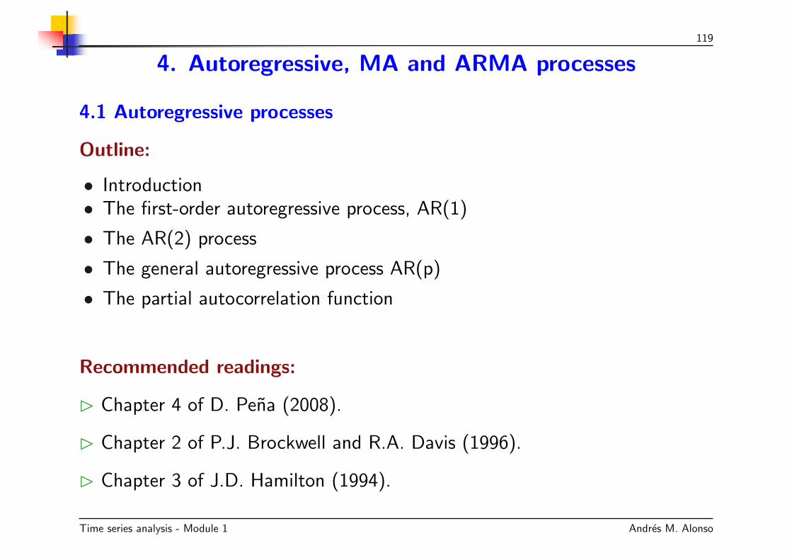
B If we consider the operator as an equation, in B the coefficient φ is calledthe factor of the equation.

B The stationarity condition is that this factor be less than the unit in absolutevalue.

B Alternatively, we can talk about the root of the equation of the operator,which is obtained by making the operator equal to zero and solving the equationwith B as an unknown;

1− φB = 0

which yields B = 1/φ.

B The condition of stationarity is then that the root of the operator be greaterthan one in absolute value.


126


Expectation

B Taking expectations in (33) assuming |φ| < 1, such that E [zt] = E[zt−1] =µ, we obtain

µ = c+ φµ

Then, the expectation (or mean) is

µ =c

1− φ(36)

Replacing c in (33) with µ(1− φ), the process can be written in deviations tothe mean:

zt − µ = φ (zt−1 − µ) + at

and letting zt = zt − µ,zt = φzt−1 + at (37)

which is the most often used equation of the AR(1).


127


Variance

B The variance of the process is obtained by squaring the expression (37) andtaking expectations, which gives us:

E(z2t ) = φ2E(z2

t−1) + 2φE(zt−1at) + E(a2t ).

We let σ2z be the variance of the stationary process. The second term of this

expression is zero, since as zt−1 and at are independent and both variableshave null expectation. The third is the variance of the innovation, σ2, and weconclude that:

σ2z = φ2σ2

z + σ2,

from which we find that the variance of the process is:

σ2z =

σ2

1− φ2. (38)

Note that in this equation the condition |φ| < 1 appears, so that σ2z is finite

and positive.


128


B It is important to differentiate the marginal distribution of a variable fromthe conditional distribution of this variable in the previous value. The marginaldistribution of each observation is the same, since the process is stationary: ithas mean µ and variance σ2

z. Nevertheless, the conditional distribution of zt ifwe know the previous value, zt−1, has a conditional mean:

E(zt|zt−1) = c+ φzt−1

and variance σ2, which according to (38), is always less than σ2z.

B If we know zt−1 it reduces the uncertainty in the estimation of zt, and thisreduction is greater when φ2 is greater.

B If the AR parameter is close to one, the reduction of the variance obtainedfrom knowledge of zt−1 can be very important.


129


Autocovariance function

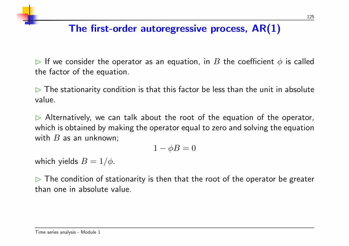
B Using (37), multiplying by zt−k and taking expectations gives us γk, thecovariance between observations separated by k periods, or the autocovarianceof order k:

γk = E [(zt−k − µ) (zt − µ)] = E [zt−k (φzt−1 + at)]

and as E [zt−kat] = 0, since the innovations are uncorrelated with the pastvalues of the series, we have the following recursion:

γk = φγk−1 k = 1, 2, ... (39)

where γ0 = σ2z.

B This equation shows that since |φ| < 1 the dependence between observationsdecreases when the lag increases.

B In particular, using (38):


130

γ1 =φσ2

1− φ2(40)


131


Autocorrelation function, ACF

B Autocorrelations contain the same information as the autocovariances, withthe advantage of not depending on the units of measurement. From hereon we will use the term simple autocorrelation function (ACF) to denote theautocorrelation function of the process in order to differentiate it from otherfunctions linked to the autocorrelation that are defined at the end of thissection.

B Let ρk be the autocorrelation of order k, defined by: ρk = γk/γ0, using(39), we have:

ρk = φγk−1/γ0 = φρk−1.

Since, according to (38) and (40), ρ1 = φ, we conclude that:

ρk = φk (41)

and when k is large, ρk goes to zero at a rate that depends on φ.


132


Autocorrelation function, ACF

B The expression (41) shows that the autocorrelation function of an AR(1)process is equal to the powers of the AR parameter of the process and decreasesgeometrically to zero.

B If the parameter is positive the linear dependence of the present on pastvalues is always positive, whereas if the parameter is negative this dependenceis positive for even lags and negative for odd ones.

B When the parameter is positive the value at t is similar to the value at t−1,due to the positive dependence, thus the graph of the series evolves smoothly.Whereas, when the parameter is negative the value at t is, in general, theopposite sign of that at t− 1, thus the graph shows many changes of signs.


133

Autocorrelation function - Example

0 50 100 150 200-3

-2

-1

0

1

2

3Parameter, φ = -0.5

5 10 15 20-0.5

0

0.5

1

Lag

Sam

ple

Auto

corr

ela

tion

Parameter, φ = -0.5

0 50 100 150 200-4

-2

0

2

4Parameter, φ = +0.7

5 10 15 20-0.5

0

0.5

1

Lag

Sam

ple

Auto

corr

ela

tion

Parameter, φ = +0.7


134

Representation of an AR(1) processas a sum of innovations

B The AR(1) process can be expressed as a function of the past values of theinnovations. This representation is useful because it reveals certain propertiesof the process. Using zt−1 in the expression (37) as a function of zt−2, wehave

zt = φ(φzt−2 + at−1) + at = at + φat−1 + φ2zt−2.

If we now replace zt−2 with its expression as a function of zt−3, we obtain

zt = at + φat−1 + φ2at−2 + φ3zt−2

and repeatedly applying this substitution gives us:

zt = at + φat−1 + φ2at−2 + ....+ φt−1a1 + φtz1

B If we assume t to be large, since φt will be close to zero we can representthe series as a function of all the past innovations, with weights that decreasegeometrically.


135


B Other possibility is to assume that the series starts in the infinite past:

zt =∑∞

j=0φjat−j

and this representation is denoted as the infinite order moving average, MA(∞),of the process.

B Observe that the coefficients of the innovations are precisely the coefficientsof the simple autocorrelation function.

B The expression MA(∞) can also be obtained directly by multiplying theequation (35) by the operator (1 − φB)−1 = 1 + φB + φ2B2 + . . . , thusobtaining:

zt = (1− φB)−1at = at + φat−1 + φ2at−2 + . . .


136

Representation of an AR(1) processas a sum of innovations - Example

Example 37. The figures show the monthly series of relative changes in theannual interest rate, defined by zt = log(yt/yt−1) and the ACF. The ACcoefficients decrease with the lag: the first is of order .4, the second close to.42 = .16, the third is a similar value and the rest are small and not significant.

-.15

-.10

-.05

.00

.05

.10

.15

88 89 90 91 92 93 94 95 96 97 98 99 00 01

Relative changes in the annual interest rates, Spain 1 2 3 4 5 6 7 8 9 10-0.2

0

0.2

0.4

0.6

0.8

Lag

Sam

ple

Auto

corr

ela

tion

Datafile interestrates.wf1


137

The AR(2) process

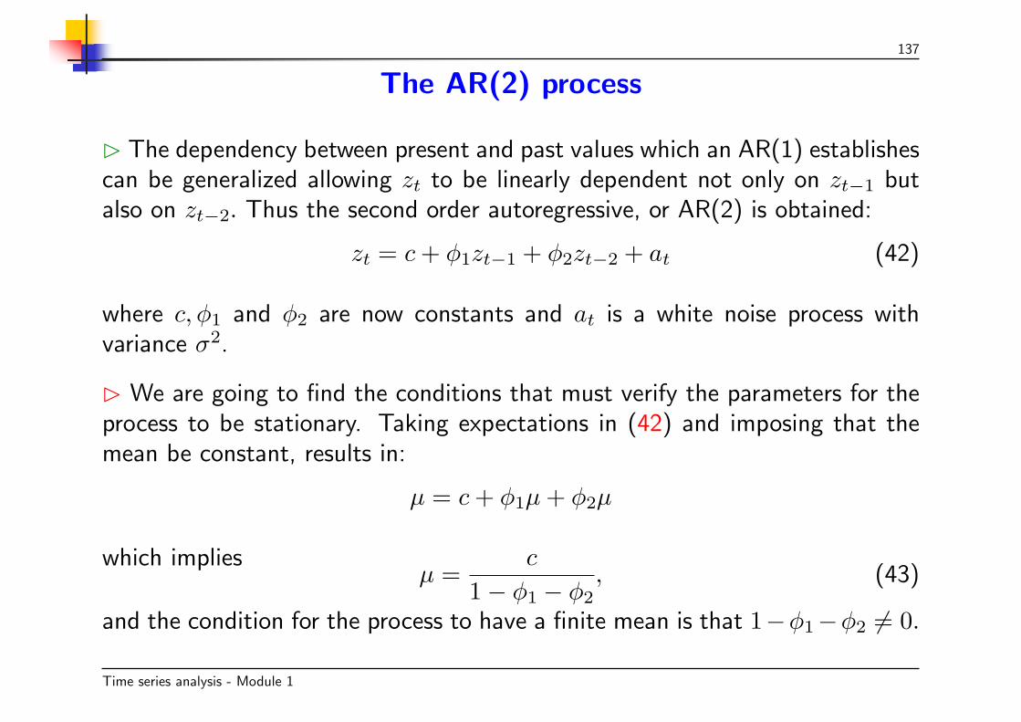
B The dependency between present and past values which an AR(1) establishescan be generalized allowing zt to be linearly dependent not only on zt−1 butalso on zt−2. Thus the second order autoregressive, or AR(2) is obtained:

zt = c+ φ1zt−1 + φ2zt−2 + at (42)

where c, φ1 and φ2 are now constants and at is a white noise process withvariance σ2.

B We are going to find the conditions that must verify the parameters for theprocess to be stationary. Taking expectations in (42) and imposing that themean be constant, results in:

µ = c+ φ1µ+ φ2µ

which impliesµ =

c

1− φ1 − φ2, (43)

and the condition for the process to have a finite mean is that 1−φ1−φ2 6= 0.


138

The AR(2) process

B Replacing c with µ(1 − φ1 − φ2) and letting zt = zt − µ be the process ofdeviations to the mean, the AR(2) process is:

zt = φ1zt−1 + φ2zt−2 + at. (44)

B In order to study the properties of the process it is advisable to use theoperator notations. Introducing the lag operator, B, the equation of thisprocess is:

(1− φ1B − φ2B2)zt = at. (45)

B The operator (1− φ1B − φ2B2) can always be expressed as (1−G1B)(1−

G2B), where G−11 and G−1

2 are the roots of the equation of the operatorconsidering B as a variable and solving

1− φ1B − φ2B2 = 0. (46)


139

The AR(2) process

B The equation (46) is called the characteristic equation of the operator.

B G1 and G2 are also said to be factors of the characteristic polynomial of theprocess. These roots can be real or complex conjugates.

B It can be proved that the condition of stationarity is that |Gi| < 1 , i = 1, 2.

B This condition is analogous to that studied for the AR(1).

B Note that this result is consistent with the condition found for the mean tobe finite. If the equation

1− φ1B − φ2B2 = 0

has a unit root it is verified that 1 − φ1 − φ2 = 0 and the process is notstationary, since it does not have a finite mean.


140

The AR(2) process


B Squaring expression (44) and taking expectations, we find that the variancemust satisfy:

γ0 = φ21γ0 + φ2

2γ0 + 2φ1φ2γ1 + σ2. (47)

B In order to calculate the autocovariance, multiplying the equation (44) by

zt−k and taking expectations, we obtain:

γk = φ1γk−1 + φ2γk−2. k ≥ 1 (48)

B Specifying this equation for k = 1, since γ−1 = γ1, we have

γ1 = φ1γ0 + φ2γ1,

which provides γ1 = φ1γ0/(1−φ2). Using this expression in (47) results in theformula for the variance:

σ2z = γ0 =

(1− φ2)σ2

(1 + φ2) (1− φ1 − φ2) (1 + φ1 − φ2). (49)


141

The AR(2) process


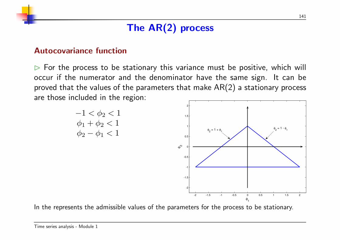
B For the process to be stationary this variance must be positive, which willoccur if the numerator and the denominator have the same sign. It can beproved that the values of the parameters that make AR(2) a stationary processare those included in the region:

−1 < φ2 < 1φ1 + φ2 < 1φ2 − φ1 < 1

-2 -1.5 -1 -0.5 0 0.5 1 1.5 2

-2

-1.5

-1

-0.5

0

0.5

1

1.5

2

φ1

φ2

φ2 = 1 - φ

1φ2 = 1 + φ

1

In the represents the admissible values of the parameters for the process to be stationary.


142

The AR(2) process

B In this process it is important again to differentiate the marginal andconditional properties. Assuming that the conditions of stationarity are verified,the marginal mean is given by

µ =c

1− φ1 − φ2

and the marginal variance is

σ2z =

(1− φ2)σ2

(1 + φ2) (1− φ1 − φ2) (1 + φ1 − φ2).

B Nevertheless, the conditional mean of zt given the previous values is:

E(zt|zt−1, zt−2) = c+ φ1zt−1 + φ2zt−2

and its variance will be σ2, the variance of the innovations which will alwaysbe less than the marginal variance of the process σ2

z.


143

The AR(2) process

Autocorrelation function

B Dividing by the variance in equation (48), we obtain the relationship betweenthe autocorrelation coefficients:

ρk = φ1ρk−1 + φ2ρk−2 k ≥ 1 (50)

specifying (50) for k = 1, as in a stationary process ρ1 = ρ−1, we obtain:

ρ1 =φ1

1− φ2(51)

and specifying (50) for k = 2 and using (51):

ρ2 =φ2

1

1− φ2+ φ2. (52)


144

The AR(2) process


B For k ≥ 3 the autocorrelation coefficients can be obtained recursivelystarting from the difference equation (50). It can be proved that the generalsolution to this equation is:

ρk = A1Gk1 +A2G

k2 (53)

where G1 and G2 are the factors of the characteristic polynomial of theprocess and A1 and A2 are constants to be determined from the initialconditions ρ0 = 1, (which implies A1+ A2 = 1) and ρ1 = φ1/ (1− φ2).

B According to (53) the coefficients ρk will be less than or equal to the unit if|G1| < 1 and |G2| < 1, which are the conditions of stationarity of the process.


145

The AR(2) process


B If the factors G1 and G2 are complex of type a± bi, where i =√−1, then

this condition is√a2 + b2 < 1. We may find ourselves in the following cases:

1. The two factors G1 and G2 are real. The decrease of (53)is the sum of the two exponentials and the shape of theautocorrelation function will depend on whether G1 and G2

have equal or opposite signs.

2. The two factors G1 and G2 are complex conjugates. It is provedin Appendix 4.1 that the function ρk will decrease sinusoidally.

B The four types of possible autocorrelation functions for an AR(2) are shownin the next figure.


146

Autocorrelation function - Examples

5 10 15 20-0.5

0

0.5

1

Sam

ple

Auto

corr

ela

tion

Real roots = 0.75 and 0.5

5 10 15 20

-0.5

0

0.5

Lag

Sam

ple

Auto

corr

ela

tion

Real roots = -0.75 and 0.5

5 10 15 20

-0.5

0

0.5

Sam

ple

Auto

corr

ela

tion

Complex roots = 0.25 ± 0.5i

5 10 15 20

-0.5

0

0.5

Lag

Sam

ple

Auto

corr

ela

tion

Complex roots = -0.25 ± 0.5i


147


B The AR(2) process can be represented, as with an AR(1), as a linearcombination of the innovations. Writing (45) as

(1−G1B)(1−G2B)zt = at

and inverting these operators, we have

zt = (1 +G1B +G21B

2 + ...)(1 +G2B +G22B

2 + ...)at (54)

which leads to the MA(∞) expression of the process:

zt = at + ψ1at−1 + ψ2at−2 + ... (55)

B We can obtain the coefficients ψi as a function of the roots equating powersof B in (54) and (55).


148


B We can also obtain the coefficients ψi as a function of the coefficients φ1 andφ2. Letting ψ(B) = 1+ψ1B+ψ2B

2 + ... since ψ(B) = (1−φ1B−φ2B2)−1,

we have (1− φ1B − φ2B2)(1 + ψ1B + ψ2B

2 + ...) = 1. (56)

B Imposing the restriction that all the coefficients of the powers of B in (56)are null, the coefficient of B in this equation is ψ1−φ1, which implies ψ1 = φ1.The coefficient of B2 is ψ2 − φ1ψ1 − φ2, which implies the equation:

ψk = φ1ψk−1 + φ2ψk−2 (57)

for k = 2, since ψ0 = 1. The coefficients of Bk for k ≥ 2 verify the equation(57) which is similar to the one that must verify the autocorrelation coefficients.

B We conclude that the shape of the coefficients ψi will be similar to that ofthe autocorrelation coefficients.


149

Representation of an AR(2) processas a sum of innovations - Examples

Example 38. The figures show the number of mink sighted yearly in an areaof Canada and the ACF. The series shows a cyclical evolution that could beexplained by an AR(2) with negative roots corresponding to the sinusoidalstructure of the autocorrelation.

0

20000

40000

60000

80000

100000

120000

50 55 60 65 70 75 80 85 90 95 00 05 10

Number of minks, Canada 2 4 6 8 10 12 14 16 18 20-0.4

-0.2

0

0.2

0.4

0.6

0.8

1

Lag

Sam

ple

Auto

corr

ela

tion


150

Representation of an AR(2) processas a sum of innovations - Examples

Example 39. Write the autocorrelation function of the AR(2) process

zt = 1.2zt−1 − 0.32zt−2 + at

B The characteristic equation of that process is:

0.32X2 − 1.2X + 1 = 0

whose solution is:

X =1.2±

√1.22 − 4× 0.320.64

=1.2± 0.4

0.64

B The solutions are G−11 = 2.5 and G−1

2 = 1.25 and the factors are G1 = 0.4and G2 = 0.8.


151

B The characteristic equation can be written:

0.32X2 − 1.2X + 1 = (1− 0.4X)(1− 0.8X).

Therefore, the process is stationary with real roots and the autocorrelationcoefficients verify:

ρk = A10.4k +A20.8k.

B To determine A1 and A2 we impose the initial conditions ρ0 = 1, ρ1 =1.2/ (1.322) = 0.91. Then, for k = 0:

1 = A1 +A2

and for k = 1,0.91 = 0.4A1 + 0.8A2

solving these equations we obtain A2 = 0.51/0.4 and A1 = −0.11/0.4.


152

B Therefore, the autocorrelation function is:

ρk = −0.110.4

0.4k +0.510.4

0.8k

which gives us the following table:

k 0 1 2 3 4 5 6 7 8ρk 1 0.91 0.77 0.63 0.51 0.41 0.33 0.27 0.21

B To obtain the representation as a function of the innovations, writing

(1− 0.4B)(1− 0.8B)zt = at

and inverting both operators:

zt = (1 + 0.4B + .16B2 + .06B3 + ...)(1 + 0.8B + .64B2 + ...)at

yields:zt = (1 + 1.2B + 1.12B2 + ...)at.


153

The general autoregressive process, AR(p)

B We say that a stationary time series zt follows an autoregressive processof order p if:

zt = φ1zt−1 + ...+ φpzt−p + at (58)

where zt = zt − µ, with µ being the mean of the stationary process zt and at

a white noise process.

B Utilizing the operator notation, the equation of an AR(p) is:

(1− φ1B − ...− φpBp) zt = at (59)

and letting φp(B) = 1 − φ1B − ... − φpBp be the polynomial of degree p in

the lag operator, whose first term is the unit, we have:

φp (B) zt = at (60)

which is the general expression of an autoregressive process.


154


B The characteristic equation of this process is define by:

φp (B) = 0 (61)

considered as a function of B.

B This equation has p roots G−11 ,...,G−1

p , which are generally different, andwe can write:

φp (B) =p∏

i=1

(1−GiB)

such that the coefficients Gi are the factors of the characteristic equation.

B It can be proved that the process is stationary if |Gi| < 1, for all i.


155



B Operating with (58), we find that the autocorrelation coefficients of anAR(p) verify the following difference equation:

ρk = φ1ρk−1 + ...+ φpρk−p, k > 0.

B In the above sections we saw particular cases in this equation for p = 1 andp = 2. We can conclude that the autocorrelation coefficients satisfy the sameequation as the process:

φp (B) ρk = 0 k > 0. (62)

B The general solution to this equation is:

ρk =∑p

i=1AiG

ki , (63)

where the Ai are constants to be determined from the initial conditions andthe Gi are the factors of the characteristic equation.


156



B For the process to be stationary the modulus of Gi must be less than oneor, the roots of the characteristic equation (61) must be greater than one inmodulus, which is the same.

B To prove this, we observe that the condition |ρk| < 1 requires that there notbe any Gi greater than the unit in (63), since in that case, when k increasesthe term Gk

i will increase without limit.

B Furthermore, we observe that for the process to be stationary there cannotbe a root Gi equal to the unit, since then its component Gk

i would not decreaseand the coefficients ρk would not tend to zero for any lag.

B Equation (63) shows that the autocorrelation function of an AR(p) processis a mixture of exponents, due to the terms with real roots, and sinusoids, dueto the complex conjugates. As a result, their structure can be very complex.


157

Yule-Walker equations

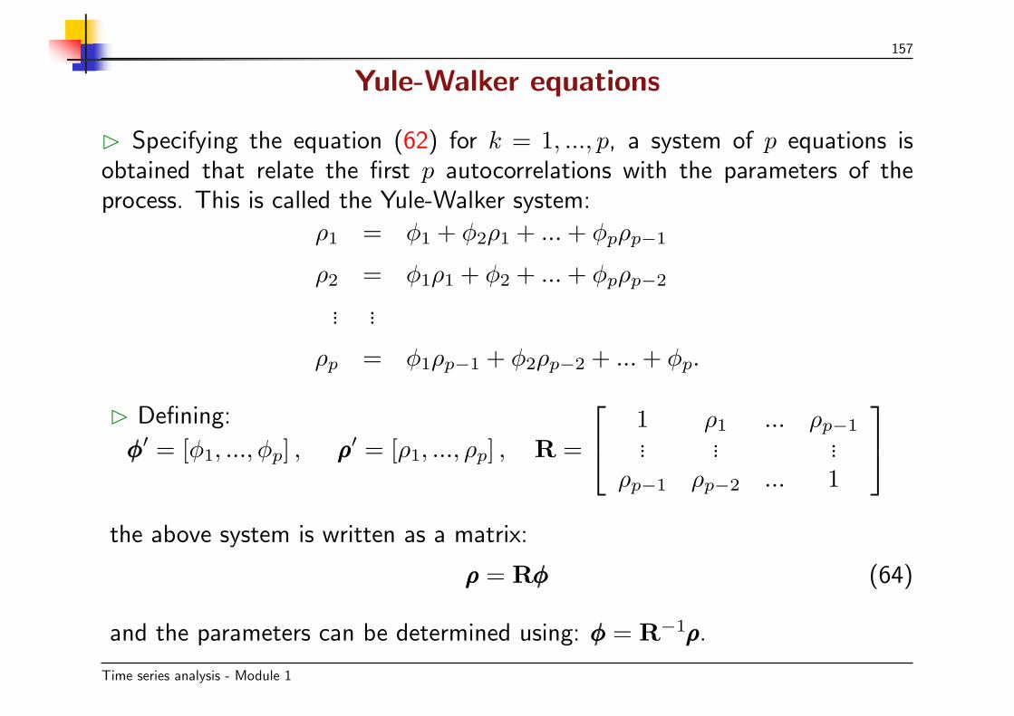
B Specifying the equation (62) for k = 1, ..., p, a system of p equations isobtained that relate the first p autocorrelations with the parameters of theprocess. This is called the Yule-Walker system:

ρ1 = φ1 + φ2ρ1 + ...+ φpρp−1

ρ2 = φ1ρ1 + φ2 + ...+ φpρp−2

... ...

ρp = φ1ρp−1 + φ2ρp−2 + ...+ φp.

B Defining:

φφφ′ = [φ1, ..., φp] , ρρρ′ = [ρ1, ..., ρp] , R =

1 ρ1 ... ρp−1... ... ...

ρp−1 ρp−2 ... 1

the above system is written as a matrix:

ρρρ = Rφφφ (64)

and the parameters can be determined using: φφφ = R−1ρρρ.


158

Yule-Walker equations - Example

Example 40. Obtain the parameters of an AR(3) process whose firstautocorrelations are ρ1 = 0.9; ρ2 = 0.8; ρ3 = 0.5. Is the process stationary?

B The Yule-Walker equation system is: 0.90.80.5

=

1 0.9 0.80.9 1 0.90.8 0.9 1

φ1

φ2

φ3

whose solution is: φ1

φ2

φ3

=

5.28 −5 0.28−5 10 −50.28 −5 5.28

0.90.80.5

=

0.891

−1.11

.


159

B As a result, the AR(3) process with these correlations is:(1− 0.89B −B2 + 1.11B3

)zt = at.

BTo prove that the process is stationary we have to calculate the factors of thecharacteristic equation. The quickest way to do this is to obtain the solutionsto the equation

X3 − 0.89X2 −X + 1.11 = 0

and check that they all have modulus less than the unit.

BThe roots of this equation are −1.7930, 0.4515 + 0.6444i and 0.4515 −0.6444i.

BThe modulus of the complex roots are less than the unit, but the real factoris greater than the unit, thus we conclude that there is no AR(3) stationaryprocess that has these three autocorrelation coefficients.


160

Representation of an AR(p) processas a sum of innovations

B To obtain the coefficients of the representation MA(∞) form we use:

(1− φ1B − ...− φpBp)(1 + ψ1B + ψ2B

2 + ...) = 1

and the coefficients ψi are obtained by setting the powers of B equal to zero.

B It is proved that they must verify the equation

ψk = φ1ψk−1 + ...+ φpψk−1

which is analogous to that which verifies that autocorrelation coefficients ofthe process.

B As mentioned earlier, the autocorrelation coefficients, ρk, and the coefficientsof the structure MA(∞) are not identical: although both sequences satisfy thesame difference equation and take the form

∑AiG

ki , the constants Ai depend

on the initial conditions and will be different in both sequences.


161

The partial autocorrelation function

B Determining the order of an autoregressive process from its autocorrelationfunction is difficult. To resolve this problem the partial autocorrelation functionis introduced.

B If we compare an AR(l) with an AR(2) we see that although in both processeseach observation is related to the previous ones, the type of relationship betweenobservations separated by more that one lag is different in both processes:

• In the AR(1) the effect of zt−2 on zt is always through zt−1, and givenzt−1, the value of zt−2 is irrelevant for predicting zt.

• Nevertheless, in an AR(2) in addition to the effect of zt−2 which istransmitted to zt through zt−1, there exists a direct effect on zt−2 on zt.

B In general, an AR(p) has direct effects on observations separated by 1, 2, ..., plags and the direct effects of the observations separated by more than p lagsare null.


162


B The partial autocorrelation coefficient of order k, denoted by ρpk, is

defined as the correlation coefficient between observations separated by kperiods, when we eliminate the linear dependence due to intermediate values.

1. We eliminate from zt, the effect of zt−1, ..., zt−k+1 using the regression:

zt = β1zt−1 + ...+ βk−1zt−k+1 + ut,

where the variable ut contains the part of zt not common to zt−1,...,zt−k+1.

2. We eliminate the effect of zt−1, ..., zt−k+1from zt−k using the regression:

zt−k = γ1zt−1 + ...+ γk−1zt−k+1 + vt,

where, again, vt contains the part of zt−1 not common to the intermediateobservations.

3. We calculate the simple correlation coefficient between ut and vt which, bydefinition, is the partial autocorrelation coefficient of order k.


163


B This definition is analogous to that of the partial correlation coefficient inregression. It can be proved that the three above steps are equivalent to fittingthe multiple regression:

zt = αk1zt−1 + ...+ αkkzt−k + ηt

and thus ρpk = αkk.

B The partial autocorrelation coefficient of order k is the coefficient αkk ofthe variable zt−k after fitting an AR(k) to the data of the series. Therefore,if we fit the family of regressions:

zt = α11zt−1 + η1t

zt = α21zt−1 + α22zt−2 + η2t

... ... ...

zt = αk1zt−1 + ...+ αkkzt−k + ηkt

the sequence of coefficients αii provides the partial autocorrelation function.


164


B From this definition it is clear that an AR(p) process will have the firstp nonzero partial autocorrelation coefficients and, therefore, in the partialautocorrelation function (PACF) the number of nonzero coefficients indicatesthe order of the AR process.

B This property will be a key element in identifying the order of anautoregressive process.

B Furthermore, the partial correlation coefficient of order p always coincideswith the parameter φp.

B The Durbin-Levinson algorithm is an efficient method for estimating thepartial correlation coefficients.


165

The partial autocorrelation function - AR(1) models

2 4 6 8 10-0.5

0

0.5

1

Parameter, φ > 0

1 2 4 6 8 10-0.5

0

0.5

1

2 4 6 8 10-1

-0.5

0

0.5

1

Parameter, φ < 0

1 2 4 6 8 10-1

-0.5

0

0.5

1


166

The partial autocorrelation function - AR(2) models

5 10 15 20-1

0

1

φ1 > 0, φ

2 > 0

2 4 6 8 10-1

0

1

5 10 15 20-1

0

1

φ1 < 0, φ

2 > 0

2 4 6 8 10-1

0

1

5 10 15 20-1

0

1

φ1 > 0, φ

2 < 0

2 4 6 8 10-1

0

1

5 10 15 20-1

0

1

φ1 < 0, φ

2 < 0

2 4 6 8 10-1

0

1


167

The partial autocorrelation function - Examples

Example 41. The figure shows the partial autocorrelation function for theinterest rates series from example 37. We conclude that the variations ininterest rates follow an AR(1) process, since there is only one significantcoefficient.

1 2 3 4 5 6 7 8 9 10-0.2

0

0.2

0.4

0.6

0.8

Lag

Sam

ple

Part

ial A

uto

corr

ela

tions


168


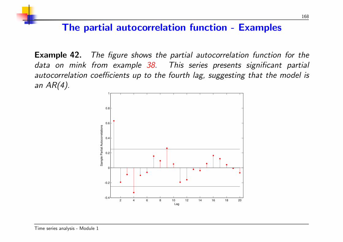
Example 42. The figure shows the partial autocorrelation function for thedata on mink from example 38. This series presents significant partialautocorrelation coefficients up to the fourth lag, suggesting that the model isan AR(4).

2 4 6 8 10 12 14 16 18 20-0.4

-0.2

0

0.2

0.4

0.6

0.8

1

Lag

Sam

ple

Part

ial A

uto

corr

ela

tions


169


Example 43. Examples 41 and 42 using EViews.

Correlogram of RC_IR1YEAR

Date: 01/29/08 Time: 19:01Sample: 1988M01 2002M03Included observations: 170

Autocorrelation Partial Correlation AC PAC Q-Stat Prob

1 0.434 0.434 32.582 0.0002 0.267 0.096 44.948 0.0003 0.281 0.168 58.800 0.0004 0.224 0.048 67.648 0.0005 0.110 -0.054 69.778 0.0006 0.016 -0.090 69.823 0.0007 0.054 0.040 70.344 0.0008 -0.014 -0.065 70.378 0.0009 0.025 0.079 70.494 0.000

10 -0.040 -0.077 70.790 0.000

Correlogram of MINKS

Date: 01/29/08 Time: 18:55Sample: 1848 1911Included observations: 64


1 0.621 0.621 25.848 0.0002 0.262 -0.202 30.511 0.0003 0.016 -0.092 30.528 0.0004 -0.256 -0.301 35.148 0.0005 -0.355 -0.037 44.178 0.0006 -0.293 0.003 50.417 0.0007 -0.086 0.188 50.961 0.0008 0.137 0.098 52.373 0.0009 0.363 0.230 62.476 0.000

10 0.419 -0.015 76.239 0.00011 0.213 -0.213 79.848 0.00012 -0.026 -0.134 79.901 0.00013 -0.192 0.024 82.948 0.00014 -0.320 -0.005 91.583 0.00015 -0.319 0.045 100.36 0.00016 -0.146 0.096 102.23 0.00017 0.068 0.041 102.64 0.00018 0.246 0.008 108.22 0.00019 0.360 0.021 120.40 0.00020 0.316 -0.003 129.97 0.000


170

Introduction

B The autoregressive processes have, in general, infinite non-zeroautocorrelation coefficients that decay with the lag. The AR processes have arelatively “long” memory, since the current value of a series is correlated withall previous ones, although with decreasing coefficients.

B This property means that we can write an AR process as a linear functionof all its innovations, with weights that tend to zero with the lag. The ARprocesses cannot represent short memory series, where the current value of theseries is only correlated with a small number of previous values.

B A family of processes that have this “very short memory” property are themoving average, or MA processes. The MA processes are a function of a finite,and generally small, number of its past innovations.

B Later, we will combine the properties of the AR and MA processes todefine the ARMA processes, which give us a very broad and flexible family ofstationary stochastic processes useful in representing many time series.


171

The first order moving average, MA(l)

B A first order moving average, MA(1), is defined by a linear combinationof the last two innovations, according to the equation:

zt = at − θat−1 (65)

where zt = zt − µ, with µ being the mean of the process and at a white noiseprocess with variance σ2.

B The MA(1) process can be written with the operator notation:

zt = (1− θB) at. (66)

B This process is the sum of the two stationary processes, at and −θat−1 and,therefore, will always be stationary for any value of the parameter, unlike theAR processes.


172

The first order moving average, MA(l)

B In these processes we will assume that |θ| < 1, so that the past innovationhas less weight than the present. Then, we say that the process is invertibleand has the property whereby the effect of past values of the series decreaseswith time.

B To justify this property, we substitute at−1 in (65) as a function of zt−1:

zt = at − θ (zt−1 + θat−2) = −θzt−1 − θ2at−2 + at

and repeating this operation for at−2 :

zt = −θzt−1 − θ2(zt−2 + θat−3) + at = −θzt−1 − θ2zt−2 − θ3at−3 + at

using successive substitutions of at−3, at−4..., etc., we obtain:

zt = −t−1∑i=1

θizt−1 − θta0 + at (67)


173

The first order moving average, MA(1)

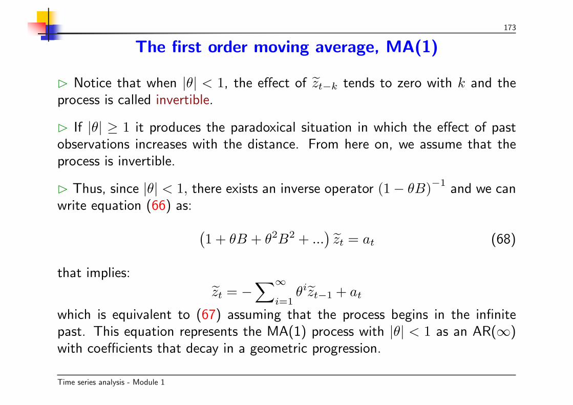
B Notice that when |θ| < 1, the effect of zt−k tends to zero with k and theprocess is called invertible.

B If |θ| ≥ 1 it produces the paradoxical situation in which the effect of pastobservations increases with the distance. From here on, we assume that theprocess is invertible.

B Thus, since |θ| < 1, there exists an inverse operator (1− θB)−1 and we canwrite equation (66) as: (

1 + θB + θ2B2 + ...)zt = at (68)

that implies:

zt = −∑∞

i=1θizt−1 + at

which is equivalent to (67) assuming that the process begins in the infinitepast. This equation represents the MA(1) process with |θ| < 1 as an AR(∞)with coefficients that decay in a geometric progression.


174


Expectation and variance

B The expectation can be derived from relation (65) which implies thatE[zt] = 0, so

E[zt] = µ.

B The variance of the process is calculated from (65). Squaring and takingexpectations, we obtain:

E(z2t ) = E(a2

t ) + θ2E(a2t−1)− 2θE(atat−1)

since E(atat−1) = 0, at is a white noise process and E(a2t ) = E(a2

t−1) = σ2,then we have that:

σ2z = σ2

(1 + θ2

). (69)

B This equation tells us that the marginal variance of the process, σ2z, is always

greater than the variance of the innovations, σ2, and this difference increaseswith θ2.


175


Simple and partial autocorrelation function

B The first order autocovariance is calculated by multiplying equation (65) byzt−1 and taking expectations:

γ1 = E(ztzt−1) = E(atzt−1)− θE(at−1zt−1).

B In this expression the first term E(atzt−1) is zero, since zt−1 depends onat−1, and at−2, but not on future innovations, such as at.

B To calculate the second term, replacing zt−1 with its expression accordingto (65), gives us

E(at−1zt−1) = E(at−1(at−1 − θat−2)) = σ2

from which we obtain:γ1 = −θσ2. (70)


176



B The second order autocovariance is calculated in the same way:

γ2 = E(ztzt−2) = E(atzt−2)− θE(at−1zt−2) = 0

since the series is uncorrelated with its future innovations the two terms arenull. The same result is obtained for covariances of orders higher than two.

B In conclusion:γj = 0, j > 1. (71)

Dividing the autocovariances (70) and (71) by expression (69) of the varianceof the process, we find that the autocorrelation coefficients of an MA(1)process verify:

ρ1 =−θ

1 + θ2, ρk = 0 k > 1, (72)

and the (ACF ) will only have one value different from zero in the first lag.


177



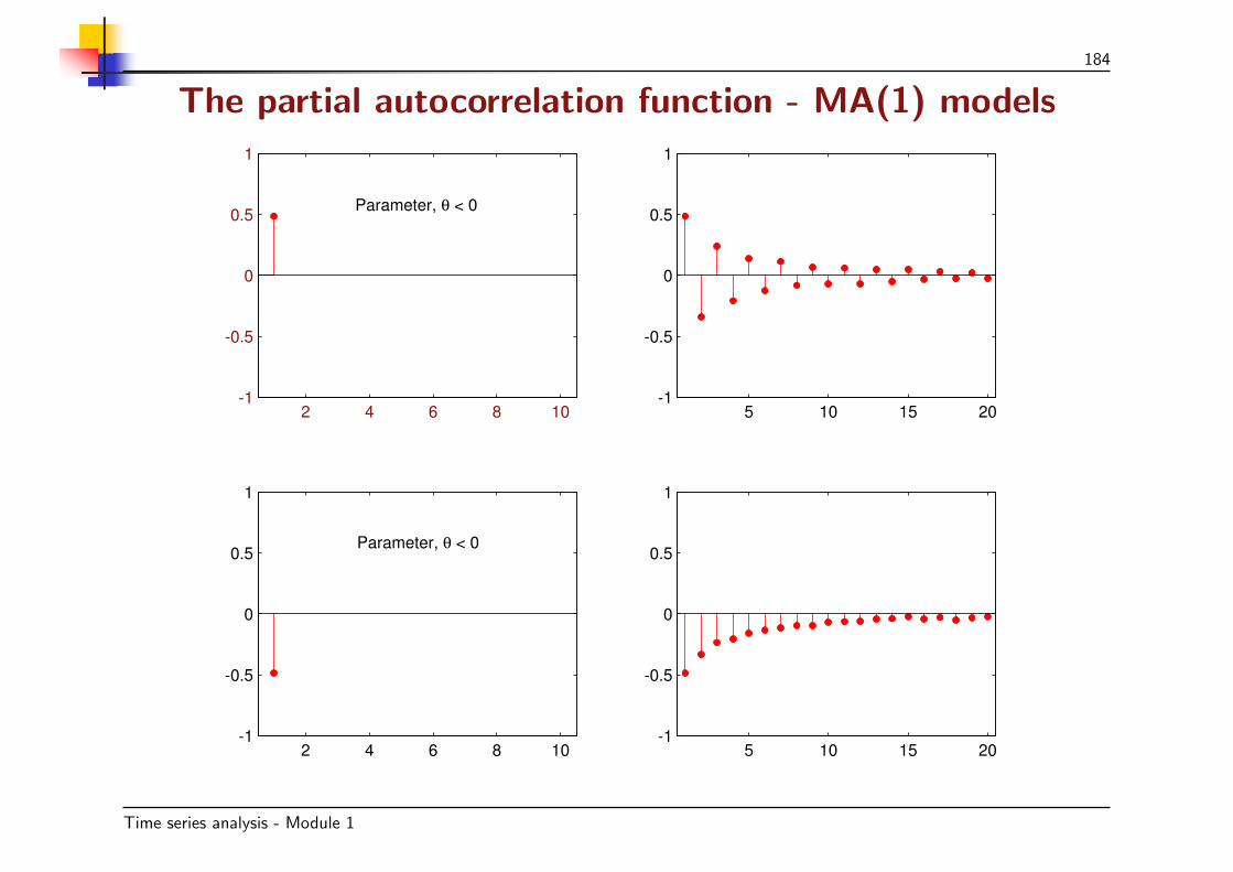
B This result proves that the autocorrelation function (ACF ) of an MA(l)process has the same properties as the partial autocorrelation function(PACF )of an AR(1) process: there is a first coefficient different from zero andthe rest are null.

B This duality between the AR(1) and the MA(1) is also seen in the partialautocorrelation function, PACF.

B According to (68), when we write an MA(1) process in autoregressive formzt−k has a direct effect on zt of magnitude θk, no matter what k is.

B Therefore, the PACF have all non-null coefficients and they decaygeometrically with k.

B This is the structure of the ACF in an AR(l) and, hence, we conclude thatthe PACF of an MA(1) has the same structure as the ACF of an AR(1).


178

Simple and partial autocorrelation function - Example

Example 44. The left figure show monthly data from the years 1881 - 2002and represent the deviation between the average temperature of a month andthe mean of that month calculated by averaging the temperatures in the 25years between 1951 and 1975. The right figure show zt = yt − yt−1, whichrepresents the variations in the Earth’s mean temperature from one month tothe next.

-1.2

-0.8

-0.4

0.0

0.4

0.8

1.2

90 00 10 20 30 40 50 60 70 80 90 00

Earth temperature (deviation to monthly mean)

-1.2

-0.8

-0.4

0.0

0.4

0.8

1.2

90 00 10 20 30 40 50 60 70 80 90 00

Earth temperature (monthly variations)


179

2 4 6 8 10 12 14 16 18 20-0.4

-0.2

0

0.2

0.4

0.6

0.8

1

Lag

Sam

ple

Auto

corr

ela

tion

2 4 6 8 10 12 14 16 18 20-0.4

-0.2

0

0.2

0.4

0.6

0.8

1

Lag

Sam

ple

Part

ial A

uto

corr

ela

tions

B In the autocorrelation function a single coefficient different from zero isobserved, and in the PACF a geometric decay is observed.

B Both graphs suggest an MA(1) model for the series of differences betweenconsecutive months, zt.


180

The MA(q) process

B Generalizing on the idea of an MA(1), we can write processes whose currentvalue depends not only on the last innovation but on the last q innovations.Thus the MA(q) process is obtained, with general representation:

zt = at − θ1at−1 − θ2at−2 − ...− θqat−q.

B Introducing the operator notation:

zt =(1− θ1B − θ2B

2 − ...− θqBq)at (73)

it can be written more compactly as:

zt = θq (B) at. (74)

B An MA(q) is always stationary, as it is a sum of stationary processes. Wesay that the process is invertible if the roots of the operator θq (B) = 0 are, inmodulus, greater than the unit.


181

The MA(q) process

B The properties of this process are obtained with the same method used forthe MA(1). Multiplying (73) by zt−k for k ≥ 0 and taking expectations, theautocovariances are obtained:

γ0 =(1 + θ21 + ...+ θ2q

)σ2 (75)

γk = (−θk + θ1θk+1 + ...+ θq−kθq)σ2 k = 1, ..., q, (76)

γk = 0 k > q, (77)

showing that an MA(q) process has exactly the first q coefficients of theautocovariance function different from zero.

B Dividing the covariances by γ0 and utilizing a more compact notation, theautocorrelation function is:

ρk =∑i=q

i=0 θiθk+i∑i=qi=0 θ

2i

, k = 1, ..., q (78)

ρk = 0, k > q,

where θ0 = −1, and θk = 0 for k ≥ q + 1.


182

The MA(q) process

B To compute the partial autocorrelation function of an MA(q) we express theprocess as an AR(∞):

θ−1q (B) zt = at,

and letting θ−1q (B) = π (B) , where:

π (B) = 1− π1B − ...− πkBk − ...

and the coefficients of π (B) are obtained imposing π (B) θq (B) = 1. We saythat the process is invertible if all the roots of θq (B) = 0 lie outside the unitcircle. Then the series π (B) is convergent.

B For invertible MA processes, setting the powers of B to zero, we find thatthe coefficients πi verify the following equation:

πk = θ1πk−1 + ....+ θqπk−q

where π0 = −1 and πj = 0 for j < 0.


183

The MA(q) process

B The solution to this difference equation is of the form∑AiG

ki , where now

the G−1i are the roots of the moving average operator. Having obtained the

coefficients πi of the representation AR(∞), we can write the MA process as:

zt =∑∞

i=1πizt−i + at.

B From this expression we conclude that the PACF of an MA is non-null forall lags, since a direct effect of zt−i on zt exists for all i. The PACF of an MAprocess thus has the same structure as the ACF of an AR process of the sameorder.

B We conclude that a duality exists between the AR and MA processes suchthat the PACF of an MA(q) has the structure of the ACF of an AR(q) andthe ACF of an MA(q) has the structure of the PACF of an AR(q).


184

The partial autocorrelation function - MA(1) models

2 4 6 8 10-1

-0.5

0

0.5

1

Parameter, θ < 0

5 10 15 20-1

-0.5

0

0.5

1

2 4 6 8 10-1

-0.5

0

0.5

1

Parameter, θ < 0

5 10 15 20-1

-0.5

0

0.5

1


185

The partial autocorrelation function - MA(2) models

2 4 6 8 10-1

0

1

θ1 > 0, θ

2 > 0

5 10 15 20-1

0

1

2 4 6 8 10-1

0

1

θ1 < 0, θ

2 > 0

5 10 15 20-1

0

1

2 4 6 8 10-1

0

1

θ1 > 0, θ

2 < 0

5 10 15 20-1

0

1

2 4 6 8 10-1

0

1

θ1 < 0, θ

2 < 0

5 10 15 20-1

0

1


186

The MA(∞) process and Wold decomposition

B The autoregressive and moving average processes are specific cases of ageneral representation of stationary processes obtained by Wold (1938).

B Wold proved that any weakly stationary stochastic process, zt, with finitemean, µ, that does not contain deterministic components, can be written as alinear function of uncorrelated random variables, at, as:

zt = µ+ at + ψ1at−1 + ψ2at−2 + ... = µ+∑∞

i=0ψiat−i (ψ0 = 1) (79)

where E(zt) = µ, and E [at] = 0; V ar (at) = σ2; E [atat−k] = 0, k > 1.

B Letting zt = zt − µ, and using the lag operator, we can write:

zt = ψ(B)at, (80)

with ψ(B) = 1 + ψ1B + ψ2B2 + ... being an indefinite polynomial in the lag

operator B.


187


B We denote (80) as the general linear representation of a non-deterministicstationary process.

B This representation is important because it guarantees that any stationaryprocess admits a linear representation.

B In general, the variables at make up a white noise process, that is, they areuncorrelated with zero mean and constant variance.

B In certain specific cases the process can be written as a function of normalindependent variables {at} . Thus the variable zt will have a normal distributionand the weak coincides with strict stationarity.

B The series zt, can be considered as the result of passing a process of impulses{at} of uncorrelated variables through a linear filter ψ (B) that determines theweight of each ”impulse” in the response.


188


B The properties of the process are obtained as in the case of an MA model.The variance of zt in (79) is:

V ar (zt) = γ0 = σ2∑∞

i=0ψ2

i (81)

and for the process to have finite variance the series{ψ2

i

}must be convergent.

B We observe that if the coefficients ψi are zero after lag q the general modelis reduced to an MA(q) and formula (81) coincides with (76).

B The covariances are obtained with

γk = E(ztzt−k) = σ2∑∞

i=0ψiψi+k,

which for k = 0 provide, as a particular case, formula (81) for the variance.

B Furthermore, if the coefficients ψi are zero after lag q on, this expressionprovides the autocovariances of an MA(q) expression.


189


B The autocorrelation coefficients are given by:

ρk =∑∞

i=0ψiψi+k∑∞i=0ψ

2i

, (82)

which generalizes the expression (78) of the autocorrelations of an MA(q).

B A consequence of (79) is that any stationary process also admitsan autoregressive representation, which can be of infinite order. Thisrepresentation is the inverse of that of Wold, and we write

zt = π1zt−1 + π2zt−2 + ...+ at,

which in operator notation is reduced to

π(B)zt = at.

B The AR(∞) representation is the dual representation of the MA(∞) and itis shown that: π(B)ψ(B) = 1 such that by setting the powers of B to zerowe can obtain the coefficients of one representation from those of another.


190

The AR and MA processes and the general process

B It is straightforward to prove that an MA process is a particular case of theWold representation, as are the AR processes.

B For example, the AR(1) process

(1− φB) zt = at (83)

can be written, multiplying by the inverse operator (1− φB)−1

zt =(1 + φB + φ2B2 + ...

)at

which represents the AR(1) process as a particular case of the MA(∞) formof the general linear process, with coefficients ψi that decay in geometricprogression.

B The condition of stationarity and finite variance, convergent series ofcoefficients ψ2

i , is equivalent now to |φ| < 1.


191


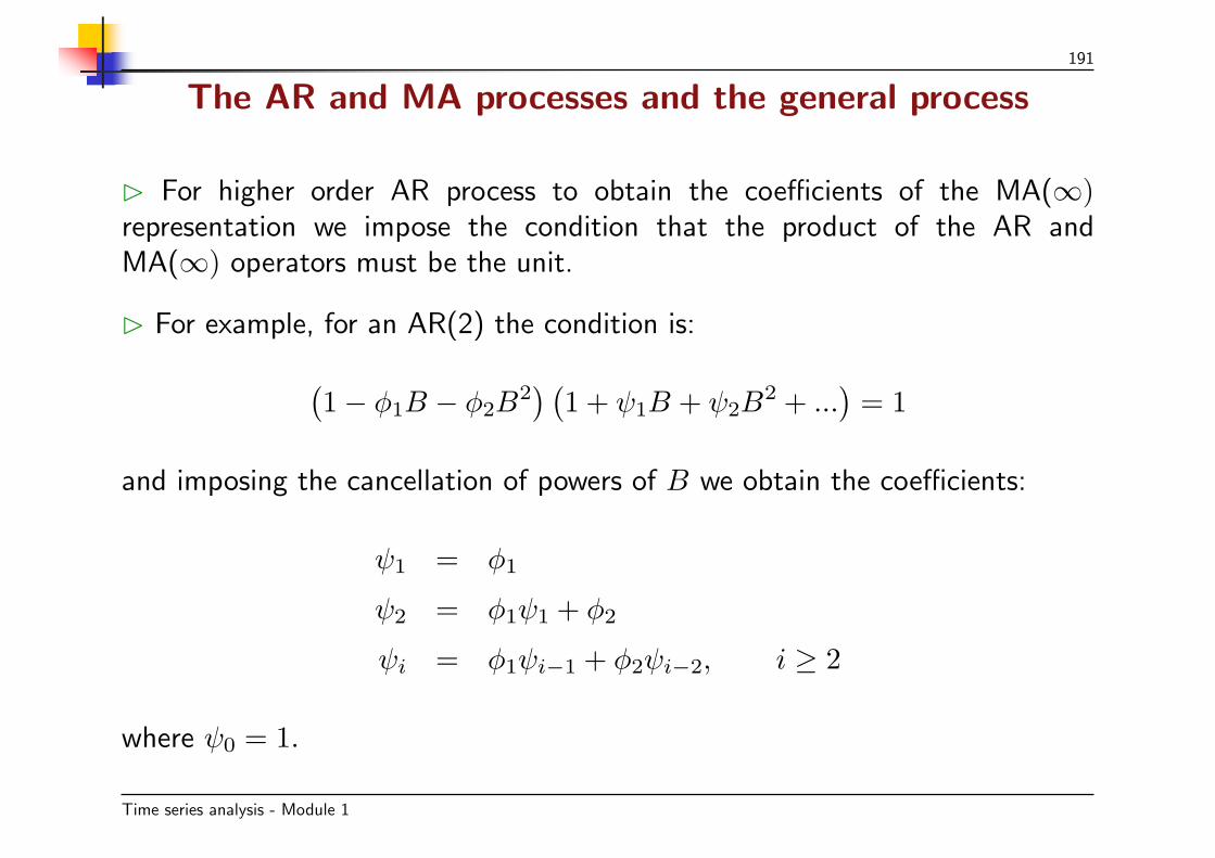
B For higher order AR process to obtain the coefficients of the MA(∞)representation we impose the condition that the product of the AR andMA(∞) operators must be the unit.

B For example, for an AR(2) the condition is:(1− φ1B − φ2B

2) (

1 + ψ1B + ψ2B2 + ...

)= 1

and imposing the cancellation of powers of B we obtain the coefficients:

ψ1 = φ1

ψ2 = φ1ψ1 + φ2

ψi = φ1ψi−1 + φ2ψi−2, i ≥ 2

where ψ0 = 1.


192


B Analogously, for an AR(p) the coefficients ψi of the general representationare calculated by:

(1− φ1B − ...− φpBp)

(1 + ψ1B + ψ2B

2 + ...)

= 1

and for i ≥ p they must verify the condition:

ψi = φ1ψi−1 + ...+ φpψi−p, i ≥ p.

B The condition of stationarity implies that the roots of the characteristicequation of the AR(p) process, φp(B) = 0, must lie outside the unit circle.


193


B Writing the operator φp(B) as:

φp (B) =∏p

i=1(1−GiB)

where G−1i are the roots of φp(B) = 0, it is shown that, expanding in partial

fractions:

φ−1p (B) =

∑ ki

(1−GiB)will be convergent if |Gi| < 1.

B Summarizing, the AR processes can be considered as particular cases of thegeneral linear process characterized by the fact that: (1) all the ψi are differentfrom zero; (2) there are restrictions on the ψi, that depend on the order of theprocess.

B In general they verify the sequence ψi = φ1ψi−1 + ...+ φpψi−p, with initialconditions that depend on the order of the process.


194

The ARMA(1,1) process

B One conclusion from the above section is that the AR and MA processesapproximate a general linear MA(∞) process from a complementary point ofview:

• The AR admit an MA(∞) structure, but they impose restrictions on thedecay patterns of the coefficients ψi.

• The MA require a number of finite terms, however, they do not imposerestrictions on the coefficients.

• From the point of view of the autocorrelation structure, the AR processesallow many coefficients different from zero, but with a fixed decay pattern,whereas the MA permit a few coefficients different from zero with arbitraryvalues.

B The ARMA processes try to combine these properties and allow us torepresent in a reduced form (using few parameters) those processes whose firstq coefficients can be any, whereas the following ones decay according to simplerules.


195


B The simplest process, the ARMA(1,1) is written as:

zt = φ1zt−1 + at − θ1at−1,

or, using operator notations:

(1− φ1B) zt = (1− θ1B) at, (84)

where |φ1| < 1 for the process to be stationary, and |θ1| < 1 for it to beinvertible.

B Moreover, we assume that φ1 6= θ1. If both parameters were identical,multiplying both parts by the operator (1− φ1B)−1

, we would have zt = at,and the process would be white noise.

B In the formulation of the ARMA models we always assume that there areno common roots in the AR and MA operators.


196


The autocorrelation function

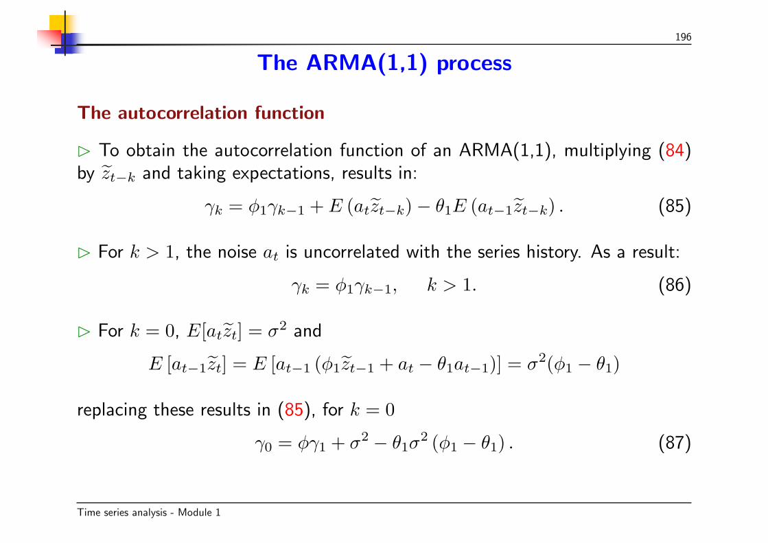
B To obtain the autocorrelation function of an ARMA(1,1), multiplying (84)by zt−k and taking expectations, results in:

γk = φ1γk−1 + E (atzt−k)− θ1E (at−1zt−k) . (85)

B For k > 1, the noise at is uncorrelated with the series history. As a result:

γk = φ1γk−1, k > 1. (86)

B For k = 0, E[atzt] = σ2 and

E [at−1zt] = E [at−1 (φ1zt−1 + at − θ1at−1)] = σ2(φ1 − θ1)

replacing these results in (85), for k = 0

γ0 = φγ1 + σ2 − θ1σ2 (φ1 − θ1) . (87)


197



B Taking k = 1 in (85), results in E[atzt−1] = 0, E[at−1zt−1] = σ2 and:

γ1 = φ1γ0 − θ1σ2, (88)

solving for (87) and (88) we obtain:

γ0 = σ21− 2φ1θ1 + θ211− φ2

1

B To compute the first autocorrelation coefficient, we divide (88) by the aboveexpression:

ρ1 =(φ1 − θ1) (1− φ1θ1)

1− 2φ1θ1 + θ21(89)

B Observe that if φ1 = θ1, this autocorrelation is zero because, as we indicatedearlier, then the operators (1− φ1B) and (1− θ1B) are cancelled out and itwill result in a white noise process.


198



B In the typical case where both coefficients are positive and φ1 > θ1 it is easyto prove that the correlation increases with (φ1 − θ1).

B The rest of the autocorrelation coefficients are obtained dividing (86) by γ0,which results in:

ρk = φ1ρk−1 k > 1 (90)

which indicates that from the first coefficient on, the ACF of an ARMA(1,1)decays exponentially, determined by parameter φ1 of the AR part.

B The difference with an AR(1) is that the decay starts at ρ1, not at ρ0 = 1,and this first value of the first order autocorrelation depends on the relativedifference between φ1 and θ1. We observe that if φ1 ≈ 1 and φ1 − θ1 = ε issmall, we can have many coefficients different from zero but they will all besmall.


199



B To calculate the PACF, we write the ARMA(1, 1) in the AR(∞) form:

(1− θ1B)−1 (1− φ1B) zt = at,

and using (1− θ1B)−1 = 1 + θ1B + θ21B2 + ..., and operating, we obtain:

zt = (φ1 − θ1) zt−1 + θ1 (φ1 − θ1) zt−2 + θ21 (φ1 − θ1) zt−3 + ...+ at.

B The direct effect of zt−k on zt decays geometrically with θk1 and, therefore,

the PACF will have a geometric decay starting from an initial value.

B In conclusion, in an ARMA(1,1) process the ACF and the PACF havea similar structure: an initial value, whose magnitude depends on φ1 − θ1,followed by a geometric decay.

B The rate of decay in the ACF depends on φ1, whereas in the PACF itdepends on θ1.


200

Autocorrelation functions - ARMA(1,1) models

5 10 15-1

-0.5

0

0.5

1

φ > 0, θ < 0

5 10 15-1

-0.5

0

0.5

1

5 10 15-1

-0.5

0

0.5

1

φ < 0, θ < 0

5 10 15-1

-0.5

0

0.5

1

Lag

5 10 15-1

-0.5

0

0.5

1

φ < 0, θ < 0

5 10 15-1

-0.5

0

0.5

1


201

Autocorrelation functions - ARMA(1,1) models

5 10 15-1

-0.5

0

0.5

1

φ < 0, θ > 0

5 10 15-1

-0.5

0

0.5

1

5 10 15-1

-0.5

0

0.5

1

φ > 0, θ > 0, θ > φ

5 10 15-1

-0.5

0

0.5

1

5 10 15-1

-0.5

0

0.5

1

φ > 0, θ > 0, θ < φ

5 10 15-1

-0.5

0

0.5

1


202

The ARMA(p,q) processes

B The ARMA (p, q) process is defined by:

(1− φ1B − ...− φpBp) zt = (1− θ1B − ...− θqB

q) at (91)

or, in compact notation,

φp (B) zt = θq (B) at.

B The process is stationary if the roots of φp (B) = 0 are outside the unitcircle, and invertible if those of θq (B) = 0 are.

B We also assume that there are no common roots that can be cancelledbetween the AR and MA operators.


203


B To obtain the coefficients ψi of the general representation of the MA(∞)model we write:

zt = φp (B)−1θq (B) at = ψ (B) at

and we equate the powers of B in ψ (B)φp (B) to those of θq (B).

B Analogously, we can represent an ARMA(p, q) as an AR(∞) model making:

θ−1q (B)φp (B) zt = π (B) zt = at

and the coefficients πi will be the result of φp (B) = θq (B)π (B).

Example


204



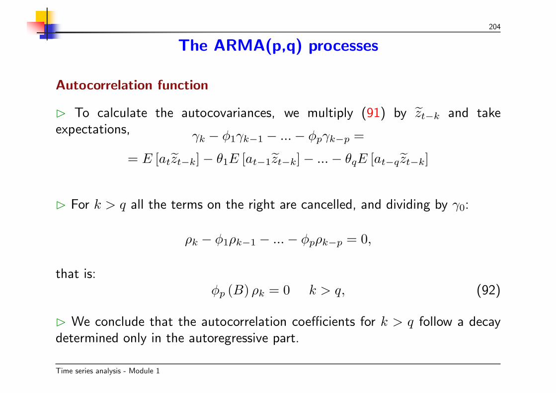
B To calculate the autocovariances, we multiply (91) by zt−k and takeexpectations, γk − φ1γk−1 − ...− φpγk−p =

= E [atzt−k]− θ1E [at−1zt−k]− ...− θqE [at−qzt−k]

B For k > q all the terms on the right are cancelled, and dividing by γ0:

ρk − φ1ρk−1 − ...− φpρk−p = 0,

that is:φp (B) ρk = 0 k > q, (92)

B We conclude that the autocorrelation coefficients for k > q follow a decaydetermined only in the autoregressive part.


205



B The first q coefficients depend on the MA and AR parameters and of those,p provide the initial values for the later decay (for k > q) according to (92).Therefore, if p > q all the ACF will show a decay dictated by (92).

B To summarize, the ACF :

• have q − p + 1 initial values with a structure that depends on the AR andMA parameters;

• they decay starting from the coefficient q − p as a mixture of exponentialsand sinusoids, determined exclusively by the autoregressive part.

B It can be proved that the PACF have a similar structure.


206

Summary

B The ACF and PACF of the ARMA processes are the result of superimposingtheir AR and MA properties:

• In the ACF certain initial coefficients that depend on the order of the MApart and later a decay dictated by the AR part.

• In the PACF initial values dependent on the AR order followed by the decaydue to the MA part.

• This complex structure makes it difficult in practice to identify the order ofan ARMA process.

ACF PACFAR(p) Many non-null coefficients first p non-null, the rest 0MA(q) first q non-null, the rest 0 Many non-null coefficientsARMA(p,q) Many non-null coefficients Many non-null coefficients


207

ARMA processes and the sum of stationary processes

B One reason that explains why the ARMA processes are frequently found inpractice is that summing AR processes results in an ARMA process.

B To illustrate this idea, we take the simplest case where we add white noiseto an AR(1) process. Let

zt = yt + vt (93)

where yt = φyt−1 + at follows an AR(1) process of zero mean and vt is whitenoise independent of at, and thus of yt.

B Process zt can be interpreted as the result of observing an AR(1) processwith a certain measurement error. The variance of this addition process is:

γz(0) = E(z2t ) = E

[(y2

t + v2t + 2ytvt)

]= γy(0) + σ2

v, (94)

since, as the summands are independent, the variance is the sum of the varianceof the components.


208


B To calculate the autocovariance we take into account that theautocovariances of process yt verify γy(k) = φkγy(0) and those of processvt are null. Thus, k ≥ 1,

γz(k) = E(ztzt−k) = E [(yt + vt)(yt−k + vt−k)] = γy(k) = φkγy(0),

since, due to the independence of the components, E [ytvt−k] = 0 for any kand since vt is white noise E [vtvt−k] = 0. Specifically, replacing the varianceγy(0) with its expression (94) for k = 1, we obtain:

γz(1) = φγz(0)− φσ2v, (95)

whereas for k ≥ 2γz(k) = φγz(k − 1). (96)

B If we compare equation (95) with (88), and equation (96) with (86) weconclude that process zt follows an ARMA(1,1) model with an AR parameterequal to φ. Parameter θ and the variance of the innovations of the ARMA(1,1)depend on the relationship between the variances of the summands.


209


B Indeed, letting λ = σ2v/γy(0) denote the quotient of variances between the

two summands, according to equation (95) the first autocorrelation is:

ρz(1) = φ− φλ

1 + λ

whereas by (96) the remainders verify, for k ≥ 2,

ρz(k) = φρz(k − 1).

B If λ is very small, which implies that the variance of the additional noise ormeasurement error is small, the process will be very close to an AR(1), andparameter θ will be very small.

B If λ is not very small, we have the ARMA(1,1) and the value of θ dependson λ and on φ.

B If λ → ∞, such that the white noise is dominant, the parameter θ will beequal to the value of φ and we have a white noise process.


210


B The above results can be generalized for any AR(p) process. It can beproved that:

AR(p) +AR(0) = ARMA(p, p),

and also that:

AR(p) +AR(q) = ARMA(p+ q,max(p, q))

B For example, if we add two independent AR(1) processes we obtain a newprocess, ARMA(2,1).

B The sum of MA processes is simple: by adding independent MA processeswe obtain new MA processes.


211


B Let us assume thatzt = xt + yt

where the two processes xt, yt have zero mean and follow independent MA(1)processes with covariances γx(k), γy(k), that are zero for k > 1.

B The variance of the summed process is:

γz(0) = γx(0) + γy(0), (97)

and the autocovariance of order k

E(ztzt−k) = γz(k) = E [(xt + yt)(xt−k + yt−k)] = γx(k) + γy(k).

B Therefore, all the covariances γz(k) of order higher than one will be zerobecause γx(k) and γy(k) are.


212


B Dividing the equation () by γz(0) and using (97), shows that theautocorrelations verify:

ρz(k) = ρx(k)λ+ ρy(k)(1− λ)

where:

λ =γx(0)

γx(0) + γy(0)is the relative variance of the first summand.

B In the particular case in which one of the processes is white noise we obtainan MA(1) model whose autocorrelation is smaller than that of the originalprocess. In the same way it is easy to show that:

MA(q1) +MA(q2) = MA(max(q1, q2)).


213


B For ARMA processes it is also proved that:

ARMA(p1, q1) +ARMA(p2, q2) = ARMA(a, b)where

a ≤ p1 + p2, b ≤ max(p1 + q1, p2 + q2)

B These results suggest that whenever we observe processes that are the sumof others, and some of them have an AR structure, we expect to observeARMA processes.

B This result may seem surprising at first because the majority of real seriescan be considered to be the sum of certain components, which would meanthat all real processes should be ARMA.

B Nevertheless, in practice many real series are approximated well by meansof AR or MA series.

B The explanation for this paradox is that an ARMA(q + h, q) process with qsimilar roots in the AR and MA parts can in practice be well approximated byan AR(h), due to the near cancellation of similar roots in both members.


214

Sum of stationary processes - Examples

Example 45. The figures show the autocorrelation functions of an AR(1)and an AR(0).

Correlogram of AR1



1 0.766 0.766 118.97 0.0002 0.563 -0.056 183.56 0.0003 0.443 0.075 223.75 0.0004 0.369 0.044 251.86 0.0005 0.281 -0.059 268.22 0.0006 0.226 0.042 278.85 0.0007 0.177 -0.022 285.41 0.0008 0.123 -0.037 288.60 0.0009 0.037 -0.108 288.89 0.000

10 -0.058 -0.110 289.62 0.00011 -0.097 0.030 291.61 0.00012 -0.062 0.109 292.43 0.00013 -0.022 0.046 292.54 0.00014 0.005 0.038 292.54 0.00015 -0.009 -0.068 292.56 0.00016 -0.030 -0.030 292.75 0.00017 -0.045 -0.010 293.21 0.00018 -0.046 0.006 293.68 0.00019 -0.057 -0.050 294.41 0.00020 -0.043 0.012 294.82 0.000

Correlogram of E2



1 0.019 0.019 0.0725 0.7882 -0.103 -0.103 2.2310 0.3283 -0.076 -0.072 3.4065 0.3334 -0.044 -0.053 3.8018 0.4335 0.120 0.108 6.8008 0.2366 -0.023 -0.042 6.9091 0.3297 -0.064 -0.048 7.7612 0.3548 0.055 0.066 8.4085 0.3959 0.030 0.025 8.5954 0.475

10 -0.005 -0.019 8.6004 0.57011 -0.072 -0.059 9.7150 0.55612 0.040 0.065 10.050 0.61213 0.132 0.107 13.825 0.38614 0.097 0.090 15.852 0.32315 -0.024 0.005 15.977 0.38416 -0.121 -0.073 19.214 0.25817 -0.005 0.004 19.219 0.31618 0.042 0.004 19.606 0.35519 -0.055 -0.076 20.287 0.37820 -0.034 -0.027 20.541 0.425

Datafile sumofst.wf1


215


B The figure shows the autocorrelation functions of the sum of AR(1)+AR(0).

0

4

8

12

16

-2.5 0.0 2.5 5.0

Series: SUM1

Sample 1 200

Observations 200

Mean 0.160213

Median 0.137882

Maximum 5.368475

Minimum -4.071789

Std. Dev. 1.810058

Skewness 0.165114

Kurtosis 2.661889

Jarque-Bera 1.861418

Probability 0.394274

Correlogram of SUM1



1 0.536 0.536 58.422 0.0002 0.307 0.028 77.700 0.0003 0.270 0.133 92.622 0.0004 0.234 0.052 103.94 0.0005 0.208 0.056 112.91 0.0006 0.053 -0.156 113.49 0.0007 0.004 -0.009 113.50 0.0008 0.038 0.033 113.79 0.0009 -0.000 -0.043 113.79 0.000

10 -0.079 -0.087 115.11 0.00011 -0.068 0.039 116.10 0.00012 -0.030 0.019 116.29 0.00013 -0.008 0.014 116.31 0.00014 -0.046 -0.038 116.77 0.00015 -0.090 -0.044 118.55 0.00016 -0.110 -0.079 121.21 0.00017 -0.020 0.098 121.29 0.00018 -0.023 -0.025 121.41 0.00019 -0.048 -0.003 121.93 0.00020 -0.052 -0.025 122.53 0.000


216


Example 46. The figures show the autocorrelation functions of two MA(1).Correlogram of MA1A



1 0.501 0.501 50.650 0.0002 0.072 -0.239 51.700 0.0003 0.079 0.218 52.983 0.0004 0.075 -0.090 54.146 0.0005 0.040 0.067 54.473 0.0006 -0.092 -0.204 56.211 0.0007 -0.158 0.003 61.412 0.0008 -0.059 0.017 62.141 0.0009 0.021 0.042 62.234 0.000

10 -0.005 -0.035 62.240 0.00011 -0.024 0.025 62.366 0.00012 0.061 0.088 63.153 0.00013 0.124 0.024 66.464 0.00014 0.047 -0.062 66.938 0.00015 0.028 0.084 67.108 0.00016 0.001 -0.099 67.109 0.00017 0.003 0.075 67.111 0.00018 0.031 -0.031 67.324 0.00019 -0.037 -0.014 67.621 0.00020 -0.052 0.005 68.224 0.000

Correlogram of MA1B



1 0.445 0.445 40.091 0.0002 -0.035 -0.292 40.344 0.0003 0.033 0.250 40.571 0.0004 0.092 -0.082 42.321 0.0005 0.043 0.064 42.699 0.0006 -0.041 -0.101 43.046 0.0007 -0.055 0.024 43.677 0.0008 0.002 0.001 43.678 0.0009 -0.019 -0.051 43.757 0.000

10 -0.080 -0.038 45.115 0.00011 0.010 0.103 45.137 0.00012 0.080 -0.010 46.509 0.00013 0.003 -0.024 46.512 0.00014 -0.083 -0.064 47.984 0.00015 -0.101 -0.055 50.192 0.00016 -0.075 -0.043 51.434 0.00017 -0.077 -0.055 52.743 0.00018 -0.134 -0.085 56.717 0.00019 -0.133 -0.029 60.639 0.00020 -0.050 0.001 61.199 0.000

Datafile sumofst.wf1


217


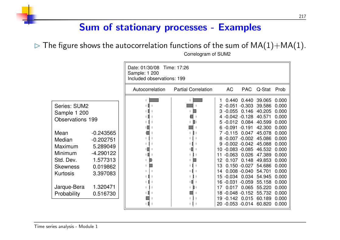
B The figure shows the autocorrelation functions of the sum of MA(1)+MA(1).

0

4

8

12

16

20

-2.5 0.0 2.5 5.0

Series: SUM2

Sample 1 200

Observations 199

Mean -0.243565

Median -0.202751

Maximum 5.289049

Minimum -4.290122

Std. Dev. 1.577313

Skewness 0.019862

Kurtosis 3.397083

Jarque-Bera 1.320471

Probability 0.516730

Correlogram of SUM2



1 0.440 0.440 39.065 0.0002 -0.051 -0.303 39.586 0.0003 -0.055 0.146 40.205 0.0004 -0.042 -0.128 40.571 0.0005 -0.012 0.084 40.599 0.0006 -0.091 -0.191 42.300 0.0007 -0.115 0.047 45.078 0.0008 -0.007 -0.002 45.086 0.0009 -0.002 -0.042 45.088 0.000

10 -0.083 -0.085 46.532 0.00011 -0.063 0.026 47.389 0.00012 0.107 0.148 49.853 0.00013 0.150 -0.027 54.686 0.00014 0.008 -0.040 54.701 0.00015 -0.034 0.034 54.945 0.00016 -0.031 -0.059 55.158 0.00017 0.017 0.065 55.220 0.00018 -0.048 -0.152 55.732 0.00019 -0.142 0.015 60.189 0.00020 -0.053 -0.014 60.820 0.000


218

Sum of stationary processes - ExamplesExample 47. The figures show the autocorrelation functions of the two sumof AR(1)+MA(1).

Correlogram of SUM3



1 0.612 0.612 75.784 0.0002 0.275 -0.161 91.114 0.0003 0.215 0.194 100.54 0.0004 0.182 -0.024 107.35 0.0005 0.149 0.061 111.95 0.0006 0.097 -0.043 113.89 0.0007 0.022 -0.047 113.99 0.0008 0.066 0.125 114.91 0.0009 0.113 0.007 117.59 0.000

10 0.066 -0.030 118.51 0.00011 0.010 -0.029 118.54 0.00012 0.059 0.107 119.29 0.00013 0.130 0.056 122.90 0.00014 0.165 0.066 128.82 0.00015 0.150 0.017 133.68 0.00016 0.119 0.018 136.76 0.00017 0.075 -0.056 138.00 0.00018 0.039 -0.032 138.32 0.00019 -0.000 -0.030 138.32 0.00020 0.019 0.071 138.41 0.000

Correlogram of SUM4



1 0.682 0.682 93.851 0.0002 0.412 -0.099 128.27 0.0003 0.353 0.210 153.63 0.0004 0.289 -0.039 170.80 0.0005 0.251 0.094 183.79 0.0006 0.235 0.022 195.23 0.0007 0.175 -0.040 201.64 0.0008 0.093 -0.063 203.45 0.0009 0.001 -0.109 203.45 0.000

10 -0.064 -0.054 204.32 0.00011 -0.006 0.136 204.33 0.00012 0.060 0.046 205.10 0.00013 0.030 -0.037 205.30 0.00014 0.011 0.026 205.32 0.00015 -0.025 -0.074 205.46 0.00016 -0.086 -0.061 207.09 0.00017 -0.135 -0.104 211.09 0.00018 -0.160 -0.071 216.72 0.00019 -0.148 -0.004 221.60 0.00020 -0.143 -0.025 226.19 0.000

Are they expectable results?


4. Autoregressive, MA and ARMA processes -...

Documents

Transcript of 4. Autoregressive, MA and ARMA processes -...