HAL Id: hal-00655386https://hal.archives-ouvertes.fr/hal-00655386

Submitted on 1 Jan 2012

HAL is a multi-disciplinary open accessarchive for the deposit and dissemination of sci-entific research documents, whether they are pub-lished or not. The documents may come fromteaching and research institutions in France orabroad, or from public or private research centers.

L’archive ouverte pluridisciplinaire HAL, estdestinée au dépôt et à la diffusion de documentsscientifiques de niveau recherche, publiés ou non,émanant des établissements d’enseignement et derecherche français ou étrangers, des laboratoirespublics ou privés.

3D Image Analysis and Artificial Intelligence for BoneDisease Classification

Abdurrahim Akgundogdu, Rachid Jennane, Gabriel Aufort, Claude-LaurentBenhamou, Osman Nuri Ucan

To cite this version:Abdurrahim Akgundogdu, Rachid Jennane, Gabriel Aufort, Claude-Laurent Benhamou, Osman NuriUcan. 3D Image Analysis and Artificial Intelligence for Bone Disease Classification. Journal of MedicalSystems, Springer Verlag (Germany), 2010, 34 (5), pp.815-828. <10.1007/s10916-009-9296-3>. <hal-00655386>

3D IMAGE ANALYSIS AND ARTIFICIAL INTELLIGENCE FOR BONE

DISEASE CLASSIFICATION

Abdurrahim Akgundogdu1, Rachid Jennane

2, Gabriel Aufort

2, Claude Laurent Benhamou

3,

Osman Nuri Ucan1

1 Istanbul University, Department of Electrical and Electronics Eng. 34850, Avcilar, Istanbul, Turkey, E-

mail:akgundog@istanbul.edu.tr

2Instiut PRISME / LESI, University of Orleans, 12, rue de Blois, 45067 Orléans Cedex 2, FRANCE

3Equipe INSERM U658, Hospital of Orleans, 1, rue Porte Madeleine, 45000 Orléans, FRANCE

Abstract

In order to prevent bone fractures due to disease and ageing of the population, and to detect problems

while still in their early stages, 3D bone micro architecture needs to be investigated and characterized.

Here, we have developed various image processing and simulation techniques to investigate bone micro

architecture and its mechanical stiffness. We have evaluated morphological, topological and mechanical

bone features using artificial intelligence methods. A clinical study is carried out on 2 populations of

arthritic and osteoporotic bone samples. The performances of Adaptive Neuro Fuzzy Inference System

(ANFIS), Support Vector Machines (SVM) and Genetic Algorithm (GA) in classifying the different

samples have been compared. Results show that the best separation success (100 %) is achieved with

Genetic Algorithm.

Keywords: Trabecular bone, Hybrid Skeleton Graph Analysis, SVM, GA, Anfis.

Introduction

The interest in three-dimensional image analysis is increasing in different fields of image

processing. In biomedical systems many new tomographic modalities now model various 3-D

images of organs and bones. Applications of these methods range from biological studies [1] to

character recognition [2]. Image analysis techniques are used in order to obtain morphological

and topological characterizations.

In the case of bone, the micro architecture plays an important role in osteoporosis, osteoarthritis

and the prediction of fractures. To characterize such material, Cruz-Orive [3] and Levitz et al. [4]

evaluated the mean size of materials by averaging 3D data. Odgaard et al. [5] and Vogel [6]

defined a connectivity index that can be computed by scanning data and storing topological

information. In addition to these methods, the morphological structure can be accessed by

determining parameters that can be computed directly from the 3D image without an underlying

model assumption [7, 8]. This work led however to global methods based on physical models that

cannot give precise information about the medium’s structure and its local properties. Nowadays,

it is possible to study the object at a local scale and obtain information from each of the elements

that compose the structure of the material [9]. A skeleton-based technique called Line Skeleton

Graph Analysis (LSGA) [10] enables the bone micro architecture to be studied at a local scale,

providing global information about the bone. This method preserves the topology of the medium

but is not suitable for structures comprising different shapes such as trabecular bone, which is

composed of rod-shaped and plate-shaped elements. In this case, all non-cylindrical shapes are

better described by 2D-surfaces rather than by 1D-curves.

We have developed a new technique called Hybrid Skeleton Graph Analysis (HSGA) [11]

to create structural models of disordered porous media. The method is based on [9], but takes into

account the shape of the object, in order to improve the geometrical approximation of [9], since

disordered porous media such as trabecular bone are not homogeneous but are composed of rod-

shaped and plate-shaped elements. Curve thinning and surface thinning are efficient respectively

for one or the other, but not for both. Our early work for skeletonizing hybrid-shaped media

focused on providing a tool for objects composed of rods and plates [10]. The HSGA method is

based on a homotopic hybrid skeleton using curve and surface thinning techniques which

preserve Betti-numbers [12]; the topology of the medium is thus perfectly preserved.

At the same time, the combination of skeletons and Finite Elements (FE) analysis to

evaluate the stiffness of large-scale porous media has recently shown great potential [13, 14]. We

have improved on a previously published beam Finite Element Analysis (FEA) in [13]. A full

protocol [15, 16] has been developed for evaluating the stiffness of large scale porous media also

based on the HSGA and using the advantage of both beam and shell Finite Elements to enable a

fast and precise mechanical simulation.

The improvement of these techniques has enabled the determination of various

parameters for quantifying the morphology and the stiffness of the bone micro architecture.

These parameters have to be combined efficiently to study bone diseases. For this purpose,

knowledge modeling is achieved using Artificial Intelligence (AI) approaches which are

developed by human expertise [17-20]. These models are based on training and testing. The

Adaptive Neuro Fuzzy Inference System (ANFIS), Support Vector Machines (SVM) and Genetic

Algorithm (GA) are the most successful tools for predicting input-output data set systems.

This work presents a study performed on 2 populations of trabecular bone samples with

an a priori knowledge of fracture risk, 9 osteoarthritic (OA) samples and 9 osteoporotic (OP)

samples. The different improved techniques have been processed on each of the 18 bone samples,

producing features which are then used to quantify the microarchitectural bone quality. These

parameters are used as entries for different artificial intelligence systems, namely: Adaptive

Neuro-Fuzzy Inference System (ANFIS), Support Vector Machines (SVM) and Genetic

Algorithm (GA). We also investigated whether the combination of these different techniques

contributes to a better prediction of the nature (OA or OP) of each sample studied.

The paper is organized as follows: first, the different artificial intelligence systems used

(ANFIS, SVM and GA) are presented. Then, the techniques used to compute the OA and OP data

are presented. The results from the clinical study follow. A discussion concludes this work.

Material and Methods

This section presents the three artificial intelligence methods, Adaptive Neuro Fuzzy Inference

System (ANFIS), Support Vector Machines (SVM) and Genetic Algorithm (GA), as well as the

image processing techniques, Hybrid Skeleton Graph Analysis (HSGA) and Finite Element

Analysis (FEA) used to classify each sample of the two studied populations (OA and OP).

1. Artificial Analysis

Artificial Intelligence (AI) is the area of computer science which deals with machine help in

finding solutions to complex problems in a more human-like fashion. This generally involves

borrowing characteristics from human intelligence, and applying them as algorithms in a

computer- friendly way.

A1

A2

B1

B2

M

M

N

N

x

y

Layer 1 Layer 2 Layer 3 Layer 4 Layer 5

W1

W2

1w

2w

x y

x y

1 1w f

2 2w f

fM

S

1.1. Adaptive Neuro-Fuzzy Inference System (ANFIS)

ANFIS is a combination of ANN and Fuzzy Inference System (FIS) [18] which is used to

determine the parameters of FIS. ANFIS implements a Takagi Sugeno Kang (TSK) [21] fuzzy

inference system in which the conclusion of the fuzzy rule is constituted by a weighted linear

combination of the crisp inputs.

1.1.1. Architecture of ANFIS

ANFIS is a fuzzy Sugeno model implemented in the framework of adaptive systems to facilitate

learning and adaptation [17]. Such a framework makes ANFIS modeling more systematic and

less reliant on expert knowledge. To present the ANFIS architecture, two fuzzy if–then rules

based on a first order Sugeno model are considered [17, 18, 21, 22].

Rule 1: If (x is A1) and (y is B1) then 1 1 1 1f p q y r , (1)

Rule 2: If (x is A2) and (y is B2) then 2 2 2 2f p q y r . (2)

where x and y are the inputs, Ai and Bi are the fuzzy sets, fi are the outputs within the fuzzy region

specified by the fuzzy rule, and i i ip , q and r are the design parameters that are determined

during the training process.

Figure 1. ANFIS architecture.

The ANFIS architecture for the implementation of these two rules is shown in Figure 1, in which

a circle indicates a fixed node, whereas a square indicates an adaptive node. In layer 1, all the

nodes are adaptive nodes. The outputs of layer 1 are the fuzzy membership grade of the input,

which are given by

1

iO =( )Ai x

, i= 1, 2, or (3)

1

iOi = 2( )B i y , i= 3, 4, (4)

where ( )Ai x , 2 ( )B i y can adopt any fuzzy membership function. We will use the Gaussian

membership function given by:

21( )

2( )

i

i

i

x c

A x e

(5)

Where c represents the membership function’s (Mfs) center and determined the Mfs width. ic

and i are parameters to be learnt. These are the premise parameters.

In layer 2, the nodes are fixed. They are labeled with M, indicating that they behave as a simple

multiplier. The outputs of this layer can be represented as

2 ( ) ( ), 1,2i ii i A BO w x y i

(6)

which are the so-called firing strengths of the rules.

In layer 3, the nodes are also fixed nodes. They are labeled with N, indicating that they

play a normalization role to the firing strengths from the previous layer. The outputs of this layer

can be represented as

3

1 2

, 1,2iii

wO w i

w w

(7)

These are the so-called normalized firing strengths.

In layer 4, the nodes are adaptive nodes. The output of each node in this layer is simply

the product of the normalized firing strength and a first-order Sugeno model. Thus, the outputs of

this layer are given by

4 ( ), 1,2i ii i i i iO w f w p x q y r i (8)

In layer 5, there is only one single fixed node labeled with S. This node performs the

summation of all incoming signals. Hence, the overall output of the model is given by

22

5 1

1 1 2

( ).

i iii i i

i

w fO w f

w w

(9)

It can be observed that there are two adaptive layers in this ANFIS architecture, namely

the first layer and the fourth layer. In the first layer, there are three modifiable

parameters , ,i i ia b c , which are related to the input membership functions. These parameters are

the so-called premise parameters.

In the fourth layer, there are also three modifiable parameters , ,i i ip q r , pertaining to the

first order Sugeno model. These parameters are called consequent parameters [22, 23].

1.1.2. Hybrid Learning Algorithm of ANFIS

The task of the learning algorithm for this architecture is to tune all the modifiable parameters,

namely , ,i i ia b c and , ,i i ip q r , in order to make the ANFIS output match with the training data.

When the premise parameters , ,i i ia b c of the membership function are fixed, the output of the

ANFIS model can be written as:

1 21 2

1 2 1 2

w wf f f

w w w w

. (10)

1 21 2.f w f w f (11)

1 21 1 1 2 2 2( ) ( ).f w p x q y r w p x q y r (12)

1 2 2 21 1 1 1 1 2 2 2( ) ( ) ( ) ( ) ( ) ( )f w x p w y q w r w x p w y q w r . (13)

Where 1 1 1 2 2 2, , , , ,p q r p q r are linear consequent parameters. When the premise parameters are not

fixed, the search space becomes larger and the convergence of the training becomes slower. A

hybrid algorithm combining the least squares method and the gradient descent method is adopted

to solve this problem [24]. The hybrid algorithm is composed of forward pass and backward pass.

The least squares method (forward pass) is used to optimize the consequent parameters with the

fixed premise parameters. [25, 26]. Once the optimal consequent parameters have been found, the

backward pass starts immediately. The gradient descent method (backward pass) is used to

optimize the premise parameters corresponding to the fuzzy sets in the input domain. The output

of the ANFIS is calculated by employing the consequent parameters found in the forward pass.

The output error is used to adapt the premise parameters by means of a standard back propagation

algorithm. It has been proven that this hybrid algorithm is highly efficient in training the ANFIS

[26, 27].

1.2. Support Vector Machines (SVM)

Support Vector Machine is an effective technique for data classification. The SVM proposed by

Vapnik [19] has been extensively studied for classification, regression and density estimation. A

classification task usually involves training and testing data which consist of some data instances.

Each sample in the training set contains one “target value” (class labels) and several “attributes”

(features). The goal of SVM is to produce a model which predicts the target value of data

instances in the testing set where only the attributes are known. Figure 2 illustrates the map of

input – output SVM space.

Figure 2. Mapping the Input and Output space.

In Figure 3, there are many possible linear classifiers that can separate the data, but there

is only one that maximizes the margin (maximizes the distance between the nearest data point of

each class). This linear classifier is termed the optimal separating hyper plane.

Figure 3. General separation of optimal hyper plane.

Based on the principle of structural risk minimization, the SVM upper bounds the

expected risk (mean error rate measured on the test set) using the sum of the empirical risk (mean

error rate measured on the training set) and a bound, called the Vapnik–Chervonenkis (VC)

confidence. In order to construct an optimal decision hypothesis, the SVM holds the empirical

risk fixed and minimizes the VC confidence by limiting the flexibility of the set of candidate

functions searched by the machine (classifier). The minimum of this upper bound is reached by

maximizing the margin between the decision hypothesis and the classes as defined using support

vectors, thereby enabling the improvement of the classifier generalization ability.

Support vector machines (SVMs) are a set of related supervised learning methods used for

classification and regression. They belong to a family of generalized linear classifiers. A special

property of SVMs is that they simultaneously minimize the empirical classification error and

maximize the geometric margin; hence they are also known as maximum margin classifiers.

Two-dimensional space that separates two classes of data shows a hyper plane is depicted in

figure 4.

Figure 4. Linear classifier and margins.

wT xi + b ≥ 1 , yi= 1 (14)

wT xi + b ≤ -1 , yi= -1

The points on the planes H1 and H2 are the support vectors. A linear classifier is defined by a

hyper plane’s normal vector w and an offset b. The decision boundary is, wT xi + b = 0 . Each of

the two half spaces defined by this hyper plane corresponds to one class, yi= sgn (wT xi + b) The

margin of a linear classifier is the minimal distance of any training point to the hyper plane.

Viewing the input data as two sets of vectors in an n-dimensional space, an SVM will

construct a separating hyper plane in that space, which maximizes the "margin" between the two

data sets. To calculate the margin, we construct two parallel hyper planes, one on each side of the

separating one, which are "pushed up against" the two data sets. Intuitively, a good separation is

achieved by the hyper plane that has the largest distance from the neighboring data points of both

classes. It is expected that the larger the margin or distance between these parallel hyper planes,

the better the generalization error of the classifier will be.

Let , , 1,2,..... , 1,1i i ix y i k y and n

ix IR be the training samples where the training

vector. ix and iy are corresponding target value. On input pattern x , the decision function of

binary classifier is;

1

( ) ( , )

k

i i i

i

f x sign y K x x b

(15)

1 0sgn( )

1 0

for uu

for u

where k is the number of learning patterns, iy is the target value of learning pattern

ix , b is a

bias, and ( , )iK x x is a kernel function which high-dimensional feature space.

The idea of the kernel function is to enable operations to be performed in the input space

rather than the potentially high dimensional feature space. Hence the inner product does not need

to be evaluated in the feature space. This provides a way of addressing the problem of

dimensionality. However, the computation is still critically dependent upon the number of

training patterns and providing a good data distribution for a high dimensional problem will

generally require a large training set. This theory is based upon Reproducing Kernel Hilbert

Spaces (RKHS) [28-30]. An inner product in feature space has an equivalent kernel in input

space, ( , ') ( ), ( ')K x x x x (16)

provided certain conditions hold. If K is a symmetric positive definite function, which satisfies

Mercer’s Conditions,

( , ') ( ), ( '),m m m

m

K x x a x x

0ma (17)

( , ') ( ) ( ') ' 0,K x x g x g x dxdx 2 ,g L (18)

then the kernel represents a legitimate inner product in feature space. Valid functions that satisfy

Mercer’s conditions are now given, which unless stated are valid for all real x and x’. A

polynomial mapping is a popular method for non- linear modeling as,

Polynomial (homogeneous): ( , ') ( . ')dk x x x x (19)

Polynomial (inhomogeneous): ( , ') ( . ' 1)dk x x x x (20)

Radial basis functions have received significant attention, most commonly with a Gaussian form:

2

2

'( , ') exp( )

2

x xk x x

(21)

Classical techniques utilizing radial basis functions employ some method of determining a subset

of centers. Typically a method of clustering is first employed to select a subset of centers. An

attractive feature of the SVM is that this selection is implicit, with each support vector

contributing one local Gaussian functions, centered at that data point.

1.3. Genetic Algorithm (GA)

This method was inspired by work first reported by Siedlecki and Sklansky [20]. The genetic

algorithm is a method for solving both constrained and unconstrained optimization problems that

is based on natural selection, the process that drives biological evolution. In recent years, the

genetic algorithms are used in many medical applications [31].

The genetic algorithm repeatedly modifies a population of individual solutions. At each

step, the genetic algorithm selects individuals at random from the current population to be parents

and uses them to produce the children for the next generation. Over successive generations, the

population "evolves" toward an optimal solution. Genetic algorithms can be applied to solve a

variety of optimization problems that are not well suited for standard optimization algorithms,

including problems in which the objective function is discontinuous, non differentiable,

stochastic, or highly nonlinear.

The genetic algorithm uses three main types of rules at each step to create the next

generation from the current population. Firstly, selection rules select the individuals, called

parents that contribute to the population at the next generation. Secondly, crossover rules

combine two parents to form children for the next generation. Finally, mutation rules apply

random changes to individual parents to form children. GA is designed to simulate the

evolutionary processes that occur in nature [32, 33].

The basic idea is derived from the Darwinian theory of survival of the fittest. Three

fundamental mechanisms drive the evolutionary process: selection, crossover and mutation

within chromosomes. As in nature, each mechanism occurs with a certain probability, allowing

for some randomness. Selection occurs on the current population by choosing the most-fit

individuals to reproduce. Reproduction, then, can result in the crossover and/or mutation of

parent genes to form new solutions. The ratio of heuristic and stochastic decisions, at best, creates

a natural balance between survival and evolution.

For each generation of the GA, individual solutions are evaluated using a fitness function.

The evaluation method is a crucial component of the selection process since offspring for the next

generation are determined by the fitness values of the present population. Figure 5 provides a

simple diagram of the iterative nature of genetic algorithms. The generational process ends when

the user-defined goal is reached. In most cases, the number of generations is a constant and is set

by the user [34].

Figure 5. Flow diagram depicting the evolutionary process of genetic algorithm.

The algorithm is;

1. Population is randomly initialized

2. Fitness of population is determined.

3. Repeating…

a) Select parents from population.

b) Perform crossover on parents creating population. c) Perform mutation of population. d) Determine fitness of population

4. until best separately is good enough.

Figure 6. General separation of two classes by GA.

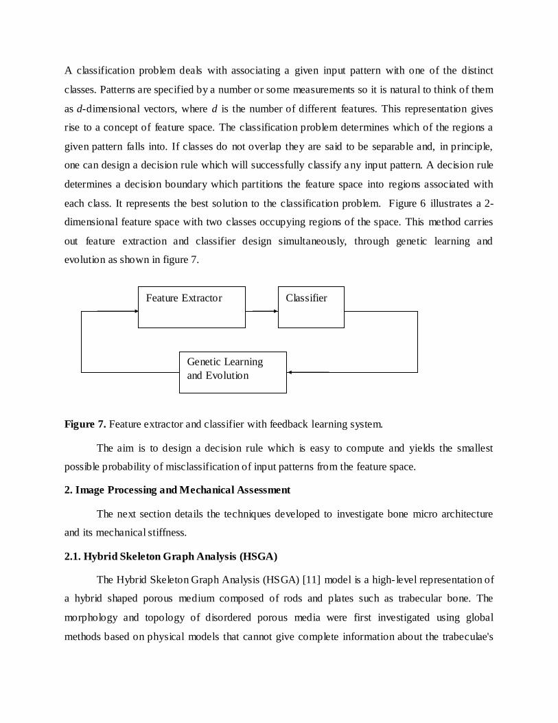
A classification problem deals with associating a given input pattern with one of the distinct

classes. Patterns are specified by a number or some measurements so it is natural to think of them

as d-dimensional vectors, where d is the number of different features. This representation gives

rise to a concept of feature space. The classification problem determines which of the regions a

given pattern falls into. If classes do not overlap they are said to be separable and, in principle,

one can design a decision rule which will successfully classify any input pattern. A decision rule

determines a decision boundary which partitions the feature space into regions associated with

each class. It represents the best solution to the classification problem. Figure 6 illustrates a 2-

dimensional feature space with two classes occupying regions of the space. This method carries

out feature extraction and classifier design simultaneously, through genetic learning and

evolution as shown in figure 7.

Figure 7. Feature extractor and classifier with feedback learning system.

The aim is to design a decision rule which is easy to compute and yields the smallest

possible probability of misclassification of input patterns from the feature space.

2. Image Processing and Mechanical Assessment

The next section details the techniques developed to investigate bone micro architecture

and its mechanical stiffness.

2.1. Hybrid Skeleton Graph Analysis (HSGA)

The Hybrid Skeleton Graph Analysis (HSGA) [11] model is a high- level representation of

a hybrid shaped porous medium composed of rods and plates such as trabecular bone. The

morphology and topology of disordered porous media were first investigated using global

methods based on physical models that cannot give complete information about the trabeculae's

Genetic Learning

and Evolution

Classifier Feature Extractor

structure and its local properties. In 2000 a new method called Line Skeleton Graph Analysis

(LSGA) [10] was introduced for studying porous media using a skeleton-based technique.

However, as it uses a curve skeleton, the LSGA has its drawbacks since all non-cylindrical

shapes are better described by 2D-surfaces rather than by 1D-curves.

a) Hybrid skeleton

The HSGA [11] relies on a new hybrid skeletonization process which is computed by processing

curve or surface thinning, depending on the local shape of the object. To switch between the 2

skeleton variants, the HSGA improves a recent algorithm [/***compléter bonnassie] which

classifies the voxels of an object according to their topological predisposition to belong to a plate

or to a rod zone [36]. Then, surface and curve thinning algorithms are applied depending on

whether each primitive belongs to the set of rods or plates. The proposed hybrid thinning

algorithm preserves connectivity which is an essential feature when characterizing porous media

such as trabecular bone. Figure 8(a) and figure 8(b) show respectively an extracted portion of a

trabecular bone sample and its hybrid skeleton.

b) Classification

Once the hybrid skeleton (figure 8(a)) has been computed, a classification step is applied to label

each voxel of the skeleton according to its structural role. The classification consists in affecting

a class identifier to each voxel of the skeleton according to its structural role. We define 4 classes

of voxels: “rod”, “line-end”, “plate” and “node”. As in [10], 2 voxels of the solid phase are

neighbors if they are 26-connex (i.e. they share at least one corner). Similarly, voxels of the pore

phase are neighbors if they are 6-connex (i.e. they share at least a face).

The voxel classification is based on a 3-step process:

1 Step 1: Initialization

All voxels are set to “plate”.

2 Step 2: Determination of rod-shaped 1D-curves

A voxel is marked as “rod” if it has only 2 solid neighbors that are not neighbors

themselves. A voxel is marked as “line-end” if it has only 1 neighbor.

3 Step 3: Determination of interfaces between elements

Any voxel is set to node if:

- It has more than 2 “rod” or “line-end” neighbors

- It is a “plate” and has a “rod” or “line-end” neighbor

Figure 8(c) shows the result of the classification step. Each voxel of the skeleton has been

marked as belonging to a “rod”, “line-end”, “plate” or “node” class.

c) Individualization

After classification, the role of each voxel in the skeleton can be determined. However, the plates

and rods of the structure cannot be processed one by one, since they have not been extracted and

individualized. In each class, the structure elements have to be marked separately. To do so, all

the information associated to one plate or rod must be collected. This is the object of the

individualization process which processes recursively all the voxels of the structure and

determines the interfaces of each element of the object. The elements individualization algorithm

is implemented as a 3-step loop:

4 Step 1: Finding a solid phase element

An initial voxel (the seed) is chosen in the classified skeleton. It can be of type

“plate” for a plate element or “rod” for a rod element.

5 Step 2: Spreading the information

The seed is recursively spread through the skeleton voxels until the element

boundaries are found. Boundary voxels can be of type “node” or “line-end”.

6 Step 3: Registering the new element

Once an element has been entirely defined, its voxels and interfaces are registered in

the model.

this information is registered in the HSGA model. Figure 8(c) illustrates how different elements

of the structure are individualized.

d) Segmentation

The classified and individualized skeleton supports a standalone use as it already contains

information about the medium. The analysis can be improved however by processing

segmentation of the original object. For this purpose, we implement a 3D region-growth iterative

process. It takes the skeleton voxels of each element as a seed and iteratively merges neighbors

from the original volume. As a result, each solid voxel of the object is finally associated to an

element of the HSGA model (plate or rod). Figure 8(d) illustrates this segmentation. All the

voxels of the original object have been referenced in the model, and the global shape is

unchanged. It can be seen that these voxels are associated to different plate or rod elements

(shown by different colors), according to the natural region growth to which they belong.

(a) (b) (c) (d)

Figure 8. Illustration of the HSGA model and its different computing steps on a trabecular bone

sample. Original trabecular bone (a), hybrid skeleton (b), classified hybrid skeleton (c), final

HSGA segmented model (d). In (b) and (c), the skeleton is stacked over the original object.

Once the HSGA model has been completed, a template of the trabecular network is

obtained. Each vertex and branch is localized, enabling the extraction of each trabecula from the

network. The HSGA model contains morphological, topological and volumetric information and

many parameters can be measured which are discussed in the clinical study. In the next section,

The HSGA is used as a basis for the generation of finite element models.

2.2. Mechanical Assessment

The reference for Finite Elements (FE) analysis of discrete samples is unquestionably voxel-to-

element conversion as discussed in many articles [37, 38]. However, in the case of skeleton-based

models, other types of elements can be used to simplify large-scale problems and prevent time

resource consumption. In this section, we explain our modeling choices, relative to the

compromise between simplification and loss of accuracy in the simulation. First, the method used

to convert rod shapes to beam chains is explained. Then the triangulation technique for

converting plate shapes to shell elements is described.

a) Rods to beam elements chains conversion

The FE that matches the geometry of a straight rod is the beam element. Its geometry is described

as a 1D segment, which is assigned a circular cross section. This technique was first investigated

in [13] to assess the stiffness of trabecular bone. However, results show that modeling the bone

by a simple rod network is not sufficient to obtain an accurate assessment of stiffness, due to

geometrical lack of accuracy. Lenthe et al. [14] explored this field of beam-modeling rod shapes

in porous media, but did not resolve the shape accuracy issues.

In order to convert a rod item to FE, we introduced the “beam chains” concept [15]. Based

on a feature extraction technique used in the field of 3D animation [39], the beam chain

introduces evenly set intermediate nodes on the curve skeleton as seen in figure 9. This process is

called “splitting” as it breaks the curve into small segments that better match the curvature of the

rod item. Finally, each split element (i.e. each effective beam FE) is assigned a section according

to the local thickness values recorded in the HSGA model, as illustrated in figure 9.

(a) (b) (c)

Figure 9. Illustration of the rods to beam elements chains conversion: voxels of the 1D path

extracted from its curve skeleton with intermediate nodes (a), simple cylinder model assumption

using the rod’s volume and skeleton length to compute its section as S = V / l (b), and beam chain

modeling of the item using local thicknesses (c)

b) Plates to shell elements conversion

Plate zones are badly described in the case of beam-only models [15, 36], which lead to a non-

negligible bias for morphological results [13]. It is suspected that this lack of geometrical

accuracy also alters mechanical results. In fact, modeling plates is much more challenging than

modeling rods, since research in this area is scanty. Recently, Lenthe et al. [14] proposed

converting a plate into a set of beams instead of a single beam. Ye t, the efficiency of this

conversion is questionable since the notion of beam set is not geometrically obvious, and the

beam sections are model-dependent. We present here an original approach that combines the

power of a new triangulation method and a better choice of FE type to improve plate modeling.

The FE used to describe planar shapes is the shell element. It is defined as a 2D medial surface

geometry (either triangle or quad strips for example), on which each element is assigned a

thickness value. The challenge in this case was to be able to transform the 26-connected plate

voxels sets into a list of simple 2D primitives such as triangles or quads. Meshing iso-surfaces

has been widely explored in computer graphics since the early 80s, leading to a great range of

techniques: surface fitting, surface tracking (also known as continuation methods) and spatial

sampling. However, the case of crossing and stacking manifold surfaces from disordered data is

still difficult to handle with criteria like Delaunay tracking, and none of these techniques suited

our needs. We chose therefore to draw on a well-known spatial sampling method: Marching

Cubes (MC) [40], which subdivides space into cells and searches those that intersect the implicit

surface. Our algorithm, called Surface Marching Cubes (SMC), computes the full- resolution

triangulation of any 26-connected surface by following the MC principle while using a new set of

neighborhood patterns. All the triangles linking the voxels of the surface are generated. Figure 10

presents the result of the triangulation of a simple 26-connex surface set. Finally, each shell

element (i.e. each triangle) is assigned a section according to the local thickness value in the

thickness map, as was done for the beam elements in the case of rod shapes.

(a) (b)

Figure 10. Illustration of the plates to shell elements conversion: 26-connex voxels of the 2D

surface extracted from its surface skeleton (a), and example of a shell elements triangulation

using Surface Marching Cubes (b).

The HSGA is used as a basis for the generation of FE models. Thickness map matching

[41] is processed to improve the geometrical accuracy of all the FE models generated, using local

cross-section values.

All the FE models were imported into the commercial software “Abaqus”, which was

used to estimate their apparent Young’s Modulus. As the simulation required material definition,

we assigned the entire model the same behavior, with a bone tissue characterized by an arbitrary

Young’s modulus of 15 GPa and a Poisson’s coefficient of 0.3. These values are close to those

found in the literature [14, 42]. In this kind of comparative study, the material’s behavior does not

really matter since the measured reaction forces are compared relatively. Once defined, each

model was tested in compression in the 3 space directions (x, y and z). Boundary conditions on

the cube’s faces were set to zero for translations perpendicular to the faces and their

complementary rotations. Complementary translations were also blocked for the 2 faces

perpendicular to the compression axis. Then, a displacement value Δl was applied on the

compression direction’s front face. A small displacement of 2% of the cube’s size (i.e. 0.0913

mm) avoided non- linearity issues. The apparent Young’s modulus (Eapp) of the model was then

computed [14] as:

2 ( / ) /( / )Eapp RF l l l (22)

where ΣRF represents the measured sum of the Reaction Forces (RF) on each node of the

compression face, and l is the size of the cube’s side.

Results

The HSGA is an efficient tool for the analysis of porous media. This section presents its

usefulness to describe trabecular bone samples from a clinical study. For this purpose, the

medical staff at the hospital of Orleans (France) provided us with 2 populations of 9 sa mples

each, extracted from post-mortem femoral head and acquired using a Sky Scan micro-scanner

with a high-resolution µ-CT (12 µm). The first 9 samples came from OsteoArthritic (OA)

patients, whose bone structure is known to be hypertrophied, increasing the bone density. The

other 9 samples were extracted from OsteoPorotic (OP) patients characterized by the

deterioration of bone micro architecture which leads to bone fragility and fracture risk. As the

characteristics of the 2 populations are previously known, they can be used to verify the

separating power of any feature that is said to reflect the bone micro architecture alterations. The

numerical samples are 4003 isotropic voxels 8-bit grey level volumes. They were pre-processed

as follows: after applying a median filter, they were binarized at the local minimum threshold

between the 2 modes of their histogram. The Hoshen-Kopelman [43] clustering algorithm was

then used to remove non-connected solid voxel sets, as there can be no isolated material in the

bone sample. Figure 11 shows 2 extracts from an OA and an OP sample. It can be seen that there

is more solid material in the OA sample.

(OA) (OP)

Figure 11. Two 643 voxels extracts from Osteoarthritis (OA) and Osteoporotic (OP) samples to

illustrate the micro architectural differences in the two trabecular bones. The solid phase (bone) is

illustrated in black while the pore phase is in white.

Using the Hybrid Skeleton Graph Analysis, topological, morphological and mechanical

features can be measured as described below.

a) Topological parameters

As the HSGA conserves the connectivity of the studied media, it is possible to measure

topological parameters such as: Connectivity (Beta1), Number of cavities of the solid phase

(Beta2), Connectivity Density (Conn.D, mm-3).

b) Morphological parameters

From a morphological point of view, the HSGA enables the following non exhaustive list of

parameters to be measured: Bone Mineral Density (BMD, defined as Bone Volume over Total

Volume, BV/TV), Bone Surface over Total Volume (BS/TV, mm-1), Bone Surface over Bone

Volume (BS/BV, mm-1), Rod Volume (Rod.V, mm3), Rod Proportion (Rod.Prop, % ), Plate

Volume (Plate.V, mm3), Plate Proportion (Plate.Prop, %), Element Number (El.N defined as

Ro.N plus Pl.N), Plate Number (Pl.N), Rod Number (Ro.N), Rod Length (Ro.L, mm), Rod

Volume (Ro.V, mm3), Rod Section (Ro.S, mm2), Rod Thickness (Ro.Th, mm), Plate Surface

(Pl.S, mm2), Plate Volume (Pl.V, mm3), Plate Thickness (Pl.Th, mm).

c) Mechanical parameters

Finally, associating the HSGA model to Finite Element Analysis allows measurement of new

features such as: Mesh Shell Number (M.Sh.N), Mesh Node Number (M.No.N), Mesh Beam

Number (M.Be.N), and Young’s Modulus (EApp(x, y, z)) in the 3 Space directions (x,x and z).

Table 1 gives all the input parameters with minimum, maximum, mean and standard deviation

values for each of the 27 parameters described above. Figure 12 shows all the input parameters’

distribution versus one output parameter value.

Table 1: Input parameters obtained from HSGA and FE Analysis.

Parameters Minimum Maximum Mean StdDev

1 Beta1 259 1650 795,111 336,375

2 Beta2 3 41 20,33 12,654

3 Conn.D -14,692 -2,294 -6,962 2,971

4 BV/TV 0,058 0,321 0,209 0,067

5 MC.BS/TV 1,418 3,946 3,194 0,634

6 MC.BS/BV 11,326 24,325 16,16 3,28

7 Rod.V 3,469 13,939 8,791 2,578

8 Rod.Prop 0,193 0,881 0,405 0,147

9 Plate.V 0,773 27,282 14,492 6,097

10 Plate.Prop 0,119 0,807 0,595 0,147

11 Shape.Ratio 0,24 7,379 1,012 1,606

12 El.N 604 3414 1,868,611 822,669

13 Ro.N 445 2438 1,448,778 589,738

14 Pl.N 37 976 419,833 253,171

15 Ro.L 0,174 0,444 0,245 0,065

16 Ro.V 0,002 0,009 0,004 0,002

17 Ro.S 0,017 0,073 0,039 0,016

18 Ro.Th 0,149 0,305 0,218 0,044

19 Pl.S 0,069 0,616 0,243 0,132

20 Pl.V 0,022 0,101 0,05 0,019

21 Pl.Th 0,163 0,361 0,266 0,054

22 Mesh.Sh.N 15376 338683 211581,39 74,493,854

23 Mesh.No.N 10292 186793 117405,94 40,368,399

24 Mesh.Be.N 791 3549 2,253,722 650,924

25 Mec.Eapp.X 3,405 265,664 72,669 60,356

26 Mec.Eapp.Y 4,856 358,696 99,122 97,839

27 Mec.Eapp.Z 11,126 164,913 76,068 43,687

a)

b)

Figure 12. Input and output parameters. a) Distribution of 27 Input parameters versus 1 Output

Parameter, b) One output Parameter of two classes (OA, OP).

Figure 12 shows that none of the computed 27 parameters is able to distinguish significantly

between the 2 populations studied. This study involves 18 samples with 27 input parameters and

1 output parameter. 12 samples are used for prediction and 6 for the test to be classified as OA or

OP with Adaptive Neuro-Fuzzy Inference System (ANFIS), Support Vector Machines (SVM)

and Genetic Algorithm (GA). Firstly we used ANFIS (Figure 13).

Figure13. Architecture of our ANFIS model: 27 inputs and 1 output with 4 rules.

In ANFIS model, Gaussian Membership Function and 5 rules were used. Therefore, 18

samples are not enough for accurate prediction with ANFIS. We could not obtain satisfactory

results and it is shown in figure 14. 18 samples are not enough for accurate prediction with

ANFIS. We could not obtain satisfactory results using ANFIS, as shown in figure 14.

Figure 14. Prediction after training, “o” is the actual value and “*” is the predicted value.

We applied the same real data group for SVM with Linear kernel function. For linear kernel C=1,

Epsilon = e-12 and tolerance parameter = 0.100 are chosen. For Genetic Algorithm; population

size is 50, crossover rate is 0.9 and mutation rate is 0.07.

Classification of OA and OP using Genetic Algorithm and SVM Algorithm are simulated for

various training- test ratios (%) of all data set such as 50-50 and 66.6-33.3. In order to obtain

better network generalization, 4-fold cross validations are also used. Table 2 lists confusion

matrix and obtained classification success rate.

Table 2. Confusion Matrix and results of simulated methods.

Methods Evaluate on

9 training and 9 testing data

4-fold cross-validation

Evaluate on

12 training and 6 testing data

SVM

OA OP Success Rate=100% OA OP Success

Rate=88.88% OA OP

Success

Rate=83.33%

4 0 OA 8 1 OA 3 0 OA

0 5 OP 1 8 OP 1 2 OP

GA

OA OP Success Rate=100% OA OP Success

Rate=94.44% OA OP

Success Rate=100%

4 0 OA 9 0 OA 3 0 OA

0 5 OP 1 8 OP 0 3 OP

Discussion

This paper presents an original association of image processing and artificial intelligence

methods for a better classification of two studied populations composed of 9 osteoarthritis and 9

osteoporosis samples denoted OA and OP respectively.

Concerning image processing, we have presented a precise assessment technique for the

3D characterization of a complex porous medium such as trabecular bone. Hybrid Skeleton

Graph Analysis (HSGA) is a technique which generates structural models of the object. It

consists in an efficient combination of curve and surface thinning techniques and considers the

local shape of each element that composes the structure of the medium. HSGA can classify each

element of the structure as rod- like or plate- like without ignoring the intersections and the

termini. Features extracted from the HSGA contain significant topological and morphological

information. The HSGA is used to extract mechanical features thanks to a finite element analysis.

Twenty-seven features are processed on each of the 18 bone samples. A comparative

discriminate analysis using artificial intelligence is applied to identify each of the samples as OA

or OP.

For the first test, Adaptive Neuro-Fuzzy Inference System (ANFIS) was used but its

success in identifying each of the samples was poor due to lack of samples and many nodes

(Figure 14). We then applied Support Vector Machines (SVM) with Linear Polynomial Kernel

and obtained a high degree of success. Finally, we used Genetic Algorithm (GA) and obtained

correct predictions and 100 % success (Table 2).

The results presented in this paper are consistent with our expectations, since geometrical

improvement in the models leads to better and more precise characterization of the structure. The

long-term aim of our work is to develop a biomechanical simulation protocol that could be used

to virtually characterize the stiffness of trabecular bone samples [16]. This will contribute

significantly to detecting bone fragilities simply by acquiring 3D images, for example with a

high-resolution in-vivo CT and simulating mechanical compression using fast and precise FE

models. Associating different techniques with artificial intelligence could be used by physicians

to complete their diagnosis efficiently. The drawback of this study is the small number o f

samples in the populations. Further work is to be carried out on larger sets of trabecular bone

samples.

References

1. Thiel, E., and Montanvert, A., Shape splitting from medial lines using the 3-4 chamfer distance, In C. Arcelli et al., editors, Visual Form Analysis and Recognition, 537-546.

Plenum, New York, 1992. 2. Gonzalez, R.C., and Woods, R.E., Digital Image Processing. Addison Wesley publisher

50803, 1992.

3. Cruz-Orive, L. M., Estimation of sheet thickness distribution from linear and plate Sections. Biomed, No; 21, pp. 717-730, 1979.

4. Levitz, P., and Tchoubar, D., Disordered porous solids: from chord distributions to small angle scattering. J. Phys, No: II 2, pp. 771-790, 1992.

5. Odgaard, A., and Gundersen, H. J. G., Quantification of connectivity in cancellous bone, with special emphasis on 3D reconstructions. Bone, No : 14, pp. 173-182, 1993.

6. Vogel, H. J., Digital unbiased estimation of the Euler-Poincaré characteristic in different

Dimensions. Acta Stereol., No: 16, pp. 97-104, 1997. 7. Hildebrand, T., and Rüegsegger, P., A new method for the model- independent assessment

of thickness in three-dimensional images. J. Microsc., Vol. 185, pp 67–75, 1997. 8. Jennane, R., Ohley, W. J., Majumdar, S., and Lemineur, G., Fractal Analysis of Bone

X-Ray Tomographic Microscopy Projections, IEEE Tans. on Med. Imag., Vol. 20, No: 5, pp. 443- 449, 2001.

9. Pothuaud, L., Orion, P., Lespessailles, E., Benhamou, C. L., and Levitz, P., A new method for three-dimensional skeleton graph analysis of porous media : application to trabecular

bone microarchitecture”, Journal of microscopy, Vol. 199 Pt. 2, pp. 149-161, 2000.

10. Aufort, G., Jennane, R., Harba, R., and Benhamou, C. L., A New 3D Shape-Dependent Skeletonization Method. Application to Porous Media. EUSIPCO-2006, Florence, Italy,

September 2006.

11. Aufort, G., Jennane, R., and Harba, R., Hybrid skeleton graph analysis of disordered porous media. Application to trabecular bone. In Proc. IEEE Int. Conf. Acou. Spee. Sig. Proc. 2007, pp. II 781–784, Toulouse, France. May 2006.

12. Morgenthaler, D. G., Three-dimensional simple points: serial erosion, parallel thinning and skeletonization. Tech. Rep. TR-1005, 1981.

13. Pothuaud, L., Rietbergen, B. V., Charlot, C., Ozhinsky, E., and Majumdar, S., A new computational efficient approach for trabecular bone analysis using beam models

generated with skeletonized graph technique. Computer Methods in Biomech. Biomed. Eng., vol. 7, no. 4, pp. 205–213, 2004

14. Lenthe, H. G., Stauber, M., and Müller, R., Specimen specific beam models for fast and

accurate prediction of human trabecular bone mechanical properties. Bone, 39(6):1182– 1189, 2006.

15. Aufort, G., Jennane, R., Harba, R., Gasser, A., Soulat, D., and Benhamou, C. L., Nouvelle approche de modélisation de milieux poreux. Application à l'os trabéculaire.

GRETSI’05, pp. 429–432, Louvain- la-Neuve, Belgium, September 2005. 16. Aufort, G., Jennane, R., Harba, R., Gasser, A., Soulat, D., and Benhamou, C. L.,

Mechanical assessment of porous media using hybrid skeleton graph analysis and finite elements. Application to trabecular bone. Proc. EUSIPCO-2007, Poznan, Poland,

September 2007. 17. Cherkassky, V., Fuzzy Inference Systems: A Critical Review, Computational Intelligence,

Soft Computing and Fuzzy-Neuro Integration with Applications of NATO ASI Series. Computer and Systems Sciences, Springer-Verlag, Chapter 3.2, pp. 177-197. Vol. 162

Berlin, 1998. 18. Jang, J., Self- learning fuzzy controllers based on temporal backpropagation. IEEE Trans.

Neural Network, vol.3 No.5, 1992.

19. Vapnik, V., The nature of statistical learning theory. New York: Springer-Verlag, 1995. 20. Siedlecki, W., and Sklansky, J., A Note on Genetic Algorithms for Large-Scale Feature

Selection. Pattern Recognition Letters, vol. 10, no. 335-347, Nov. 1989.

21. Sugeno, M., and Kang, G. T., Structure identification of fuzzy model. Fuzzy Sets and Systems 28: 15-33, 1988.

22. Sun, C.T., Rulebase structure identification in an adaptive-network-based fuzzy inference system. IEEE Trans. Fuzzy Systems, vol.2, pp. 64-73, 1994.

23. Takagi, T., and Sugeno, M., Derivation of fuzzy control rules from human operator's control actions. Proceedings of the IFAC Symposium on Fuzzy Information, Knowledge

Representation and Decision Analysis, pp. 55-60, 1983.

24. Übeyl, E. D., and Güler, I., Automatic detection of erythemato-squamous diseases using adaptive neuro-fuzzy inference systems. Computers in Biology and Medicine 35 (5): 421- 433, 2005.

25. Takagi, T., and Sugeno, M., Fuzzy identification of systems and its applications to

modeling and control. IEEE Transactions on Systems, Man and Cybernetics , vol. SMC- 15, pp.116-132, 1985.

26. Fogelman, S. F., and Herault, J., Neuro-computing: Algorithms, Architectures and Applications. NATO ASI Series in Systems and Computer Science, Springer, 227-236.

New York, 1990.

27. Broomhead, D.S. And Lowe, D., Multivariable functional interpolation and adaptive networks. Complex Syst. 2, pp. 321-355, 1988.

28. Aronszajn, N., Theory of reproducing kernels. Trans. Amer. Math. Soc. 686:337–404, 1950.

29. Girosi, F., An equivalence between sparse approximation and Support Vector Machines. A.I. Memo 1606, MIT Artificial Intelligence Laboratory, 1997.

30. Wahba, G., Spline Models for Observational Data. Series in Applied Mathematics.

Vol. 59, SIAM, Philadelphia, 1990. 31 Kilic, N. Ucan, O.N., and Osman, O., Colonic Polyp Detection in CT Colonography with

Fuzzy Rule based Template Maching. JOMS, Vol. 33:9-18, 2009.

32. Peña-Reyes, C. A., and M. Sipper, Evolutionary Computation in Medicine: an Overview. Artificial Intelligence in Medicine, 2000. 19:1-23.

33. Koza, J. R., Keane, M.A., and Streeter, M., Evolving Inventions. Scientific American, February 2003:52-59.

34. Miller, M.T., Jerebko, A. K., Malley, J. D., and Summers, R. M., Feature Selection for Computer-Aided Polyp Detection using Genetic Algorithm. SPIE Medical Imaging.

2003.

35. Pei, M., Ding, Y., Punch, W.F., and Goodman, E.D., Genetic Algorithms For Classification and Feature Extraction, Classification Society Conference , June 1995.

36. Aufort, G., Jennane, R., Harba, R., and Benhamou, C. L., Shape classification techniques for discrete 3D porous media. Application to trabecular bone. IEEE-EMBC 2007, August

2007. 37. Ulrich D., Rietbergen, B. V., Weinans, H., and Rüegsegger, P., Finite element analysis of

trabecular bone structure: a comparison of image-based meshing techniques. J. biomech., 31(12):1187–1192, 1998.

38. Bayraktar, H. H., Nonlinear micro finite element analysis of human trabecular bone. Circle 141 - Abaqus Inc., pp. 22–25, 2004.

39. Reinders, F.,. Jacobson, M. E. D., and Post, F. H., Skeleton graph generation for feature

shape description. In Proc. Data Visualization, pp. 73–82, 2000.

40. Lorensen, W. E., and Cline H. E., Marching cubes: a high resolution 3D surface construction algorithm. Computer Graphics, 21:163–169, 1987.

41. T. Hilderbrand and P. Ruegsegger, A new method for the model independent assessment of thickness in threedimensional images. Jour. of Microscopy, 185:65–67, 1997

42. Bourne, B. C. , Marjolein, C.H., and Meulen, V.D., Finite element models predict cancellous apparent modulus when tissue modulus is scaled from specimen ct-attenuation.

J Biomech., 37(5):613–621, May 2004.

43. Hoshen, J., and Kopelman, R., Percolation and cluster distribution i. cluster multiple labeling technique and critical concentration algorithm. Phys. Rev. B, 14:3438–3445, October 1976.