University of Southern Queensland Faculty of Health, Engineering and Sciences

3D Fluid Modelling of the O.O Madsen Bridge

During Flood

A dissertation submitted by

Russell Alexander Knipe

In fulfilment of the requirements of

ENG4111 / ENG4112 Research Project

Towards the degree of

Bachelor of Engineering (Civil)

Submitted:

30th October 2014

i

Abstract

The O.O. Madsen Bridge in Warwick experiences severe flood debris blockage in the

guard rails which the public believes is leading to increased flood depths upstream when

the bridge becomes overtopped by flood water. The effects of the debris blocked guard

rails were investigated in a 2D flood model of the Condamine River. The study

concluded that depths immediately upstream of the bridge decreased in the order of

0.10-0.20m with the removal of the debris blocked guardrails. Additionally, a head loss

of 0.5m was experienced over the bridge in a 100 year Average Recurrence Interval

(ARI) flood. In order to limit computational times 2D flood models are often made as

coarse as they can be while remaining accurate over a large area. While they reflect large

scale flow patterns accurately they may not be accurate for smaller objects like the O.O.

Madsen Bridge. In order to verify the findings of the 2D flood model a 3D

Computational Fluid Dynamics (CFD) model of the bridge was created. ANSYS Fluent

was used to model a section of the bridge the width of the centre to centre distance

between the piers. A 100 year ARI flood with a depth of 7m and a velocity of 1.5m/s

was chosen as the input. The Open Channel settings in the Volume of Fluid method

were used to solve the two phase flow and model the surface of the water. The

simulation was run twice; once with 100% debris blocked guard rails that allowed no

flow to pass through, and once with no guard rails, in a similar fashion to the 2D flood

model. The model found there was a 0.08m increase in depth upstream and a 0.09m

decrease in depth downstream with the debris blocked guard rails, and no change in

depth when no guard rails were present. The data shows there is certainly a change in

depth, however it was under the ±0.13m limit of confidence for the model due to the

size of the mesh. There were several other limitations to the model which include a lack

of validating data, the behaviour of the bridge as a whole and the effect of the boundary

and initialisation conditions not being tested. Plots of shear stress on the bed of the

river found that the debris blocked guard rails have an impact on the degree of erosion

experienced around the bridge pier, increasing shear stress by up to 25%. Although the

model was not able to accurately predict the change in depth it serves as a good starting

point in understanding the effect of the guard rails on flows around the O.O. Madsen

during flood.

ii

University of Southern Queensland

Faculty of Health, Engineering and Sciences

ENG4111/ENG4112 Research Project

Limitations of Use

The Council of the University of Southern Queensland, its Faculty of Health,

Engineering & Sciences, and the staff of the University of Southern Queensland, do not

accept any responsibility for the truth, accuracy or completeness of material contained

within or associated with this dissertation.

Persons using all or any part of this material do so at their own risk, and not at the risk

of the Council of the University of Southern Queensland, its Faculty of Health,

Engineering & Sciences or the staff of the University of Southern Queensland.

This dissertation reports an educational exercise and has no purpose or validity beyond

this exercise. The sole purpose of the course pair entitled “Research Project” is to

contribute to the overall education within the student’s chosen degree program. This

document, the associated hardware, software, drawings, and other material set out in the

associated appendices should not be used for any other purpose: if they are so used, it is

entirely at the risk of the user.

iii

University of Southern Queensland

Faculty of Health, Engineering and Sciences

ENG4111/ENG4112 Research Project

Certification of Dissertation

I certify that the ideas, designs and experimental work, results, analyses and conclusions

set out in this dissertation are entirely my own effort, except where otherwise indicated

and acknowledged.

I further certify that the work is original and has not been previously submitted for

assessment in any other course or institution, except where specifically stated.

Russell Alexander Knipe

0061006071

Signature

Date

iv

Acknowledgements

The author Russell Knipe would like to thank Dr Andrew Wandel for taking on an

additional student at the last minute. Andrew was more than helpful, and without his

guidance and expertise with Fluent this project would not have been possible.

Secondly I would like to thank Dr Ian Brodie, who helped with the idea and scope for

this topic. His knowledge of hydrology and flood modelling helped to find the gap in

the literature that this thesis attempts to fill.

I would like to acknowledge the project sponsor, Southern Downs Regional Council.

Without council the idea and data for this project would never have happened.

Particular thanks go to Peter See and Stephen Bell, who have provided both their time

and knowledge to help the project.

To all my friends; thanks for four of the best years of my life. It is a lot easier going into

Z Block on a beautiful sunny weekend knowing someone else is suffering there as well.

Finally, I would like to thank my family and girlfriend for their support and patience, as

they have not seen me for most of 2014.

v

Table of Contents

Abstract ............................................................................................................................................... i

Acknowledgements ....................................................................................................................... iv

Table of Contents ............................................................................................................................ v

List of Figures ............................................................................................................................... viii

List of Tables..................................................................................................................................... x

Nomenclature .................................................................................................................................. xi

Chapter 1 Introduction............................................................................................................ 1

1.1 Background.................................................................................................................. 1

1.2 Project Objectives and Scope ................................................................................... 2

1.3 Methodology Overview ............................................................................................. 3

1.4 Consequences of Project ........................................................................................... 3

1.5 Required Resources .................................................................................................... 4

1.6 Project Timeline .......................................................................................................... 4

1.7 Risk Assessment ......................................................................................................... 5

Chapter 2 Background and Literature Review .............................................................. 6

2.1 Bridge Flow Regimes ................................................................................................. 6

2.2 1D/2D Flood Models .............................................................................................. 11

2.2.1 Modelling Bridges in a 2D Flood Model ...................................................... 14

2.3 Condamine River Flood Study ............................................................................... 15

2.3.1 Modelling the O.O. Madsen in TUFLOW ................................................... 16

2.3.2 Limitations of the 2D model .......................................................................... 18

2.3.3 Removal of Guard Rails from the O.O. Madsen ........................................ 19

2.4 Debris Blockage ........................................................................................................ 21

vi

2.5 Bridge Scour .............................................................................................................. 23

2.6 CFD Modelling and Bridges ................................................................................... 25

2.7 Collapsible Guardrails .............................................................................................. 26

2.7.1 Shear Pin Style .................................................................................................. 26

2.7.2 Manually Collapsed Style ................................................................................. 28

Chapter 3 Methodology ........................................................................................................ 30

3.1 Input Data and Assumptions .................................................................................. 30

3.2 Workbench ................................................................................................................ 33

3.3 Geometry ................................................................................................................... 33

3.4 Meshing ...................................................................................................................... 36

3.5 Fluent.......................................................................................................................... 39

3.5.1 General Set Up ................................................................................................. 39

3.5.2 Models ................................................................................................................ 40

3.5.3 Cell Zone Conditions ...................................................................................... 44

3.5.4 Boundary Conditions ....................................................................................... 44

3.5.5 Initialisation ....................................................................................................... 46

3.5.6 Solution .............................................................................................................. 47

3.6 Scour Estimation ...................................................................................................... 48

3.6.1 Shear Stress In Fluent ...................................................................................... 49

3.7 Post Processing of Data .......................................................................................... 50

3.8 Model Validation ...................................................................................................... 53

Chapter 4 Results and Discussion .................................................................................... 54

4.1 Steady State Analysis ................................................................................................ 54

4.2 Volume Fraction and Surface Plots ....................................................................... 55

4.3 Stagnant Streamline and Vector Plots ................................................................... 56

4.4 Bed Shear Plots ......................................................................................................... 59

4.5 Limitations ................................................................................................................. 61

4.6 Future Work .............................................................................................................. 63

vii

Chapter 5 Conclusions and Recommendations .......................................................... 65

Chapter 6 References ............................................................................................................ 68

Project Specification .................................................................................... 70 Appendix A

Project Timeline ............................................................................................ 72 Appendix B

Risk Assessment ............................................................................................ 74 Appendix C

Model Version Log ........................................................................................ 77 Appendix D

MATLAB Code ................................................................................................. 84 Appendix E

Steady State Analysis ................................................................................... 87 Appendix F

Comparison of CFD-Post, Fluent and MATLAB Plots ...................... 89 Appendix G

Vector Plots ..................................................................................................... 96 Appendix H

viii

List of Figures

Figure 2.1 - Pressurized flow of a bridge during flood (Bradley 1978) ............................... 8

Figure 2.2 - Submerged bridge flow conditions (Federal Highway Administartion 2012)

...................................................................................................................................................... 10

Figure 2.3 - 1D/2D model velocity contours (B.C. Phillips 2005) .................................... 13

Figure 2.4 - 2D only model velocity contours (B.C. Phillips 2005) ................................... 13

Figure 2.5 - Calibration flood heights around Warwick ...................................................... 16

Figure 2.6 - O.O. Madsen Bridge flow constriction in TUFLOW .................................... 17

Figure 2.7 - 100 year ARI flood depths (Jacobs 2012) ........................................................ 20

Figure 2.8 - 100 year ARI extents after removal of O.O. Madsen guardrails (Jacobs

2012) ............................................................................................................................................ 20

Figure 2.9 - Debris blockage on the O.O. Madsen after the 2011 floods (Warwick Daily

News, 2011)................................................................................................................................ 22

Figure 2.10 - O.O. Madsen Bridge during 2010 Flood (Warwick Daily News, 2010) .... 28

Figure 3.1 - Velocity vectors over O.O. Madsen .................................................................. 31

Figure 3.2 - Depth and velocity sections from 2D flood model ........................................ 32

Figure 3.3 - Channel bed profile plot ..................................................................................... 33

Figure 3.4 - Example of bridge section .................................................................................. 34

Figure 3.5 - Final bridge geometry – with rails ..................................................................... 35

Figure 3.6 - Final bridge geometry - no rails ......................................................................... 35

Figure 3.7 - Geometry of fluid enclosure .............................................................................. 36

Figure 3.8 - Body sizing function ............................................................................................ 37

Figure 3.9 - View of entire meshed domain .......................................................................... 38

Figure 3.10 - Cross sectional view of mesh ........................................................................... 39

Figure 3.11 - Water surface body sizing function ................................................................. 41

Figure 3.12 - Phase interface at 0.48s, 1.48s, 3.48s and 5.92s ............................................. 42

Figure 3.13 - Comparison of spatial discretization solution methods for volume fraction

(ANSYS 2012) ........................................................................................................................... 43

Figure 3.14 - Interface with compressive spatial discretization specified; simulation time

14.25 seconds ............................................................................................................................. 43

Figure 3.15 - Roughness height vs shear stress ..................................................................... 50

Figure 3.16 - Distribution of nodes in 2d plane ................................................................... 52

Figure 4.1 - Volume fraction plot with blocked guardrails ................................................. 55

Figure 4.2 - Volume fraction plot with no guardrails .......................................................... 55

ix

Figure 4.3 - Stagnation line with guard rails .......................................................................... 56

Figure 4.4 - Stagnation streamline without guardrails .......................................................... 56

Figure 4.5 - Velocity vectors around bridge with guard rails blocked (top) and no guard

rails (bottom) .............................................................................................................................. 57

Figure 4.6 - Velocity vectors near bridge pier with blocked guardrails (left) and no

guardrails (right)......................................................................................................................... 58

Figure 4.7 – Topographic comparison of bed shear with blocked guardrails (left) and no

guardrails (right) Upstream is at the top of image ................................................................ 59

Figure 4.8 - Velocity vectors with blocked guardrails (top) and no guardrails (bottom).

Colour scale shows negative vertical velocity. Right is upstream. ...................................... 60

Figure C.6.1 - Risk Assessment Matrix .................................................................................. 75

Figure 6.2 - Steady state volume fraction comparison, blocked guard rails ..................... 88

Figure 6.3 - Steady state volume fraction comparison, no guardrails ................................ 88

Figure 6.4 - CFD-Post node volume fraction plot – Blocked guard rails ......................... 90

Figure 6.5 - FLUENT cell centred volume fraction plot – Blocked guard rails .............. 90

Figure 6.6 - MATLAB volume fraction plot from CFD-Post Export – Blocked guard

rails .............................................................................................................................................. 91

Figure 6.7 - MATLAB volume fraction plot from Fluent Export – Blocked guard rails

...................................................................................................................................................... 91

Figure 6.8 - Surface plot, blocked guard rails. Green and blue vertical lines represent

location of bridge ...................................................................................................................... 92

Figure 6.9 - Volume fraction and surface plot, blocked guard rails – red line represents

calculated water surface ............................................................................................................ 92

Figure 6.10 - CFD-Post node volume fraction plot – No guard rails ............................... 93

Figure 6.11 - Fluent cell centre volume fraction plot - No guard rails .............................. 93

Figure 6.12 - MATLAB volume fraction plot from CFD-Post Export – No guard rails

...................................................................................................................................................... 94

Figure 6.13 - MATLAB volume fraction plot from Fluent Export – No guard rails ..... 94

Figure 6.14 - Surface plot, no guard rails. Green and blue vertical lines represent

location of bridge ...................................................................................................................... 95

Figure 6.15 - Volume fraction and surface plot, no guard rails – red line represents

calculated water surface ............................................................................................................ 95

Figure 6.16 - Vector plot with guard rails blocked (Top) and no guard rails (Bottom) .. 97

x

List of Tables

Table 1.1 - Summary of important dates ................................................................................. 5

Table 3.1 - Roughness height vs shear stress ........................................................................ 50

xi

Nomenclature

CFD Computational Fluid Dynamics

USQ University of Southern Queensland

SDRC Southern Downs Regional Council

1D 1 Dimensional

2D 2 Dimensional

3D 3 Dimensional

ALS Aerial Laser Survey

DTM Digital Terrain Model

DTMR Department of Transport and Main Roads

AR&R Australian Rainfall and Runoff

ARI Average Recurrence Interval

VoF Volume of Fluid

Afflux The increase in upstream depth due to an obstruction of flow

1

Chapter 1

Introduction

Australia is a nation of droughts and floods. Years without rain are normally followed

by months of intense rainfall. Australia is also a very flat nation, which means rainfall

over a large catchment area can end up in a single waterway. Relatively small perennial

rivers can become enormous watercourses during large rainfall events. Given the

historic tendency for townships to form around bodies of water, these flood events can

cause considerable damage in terms of lives and property.

At the same time computers are always increasing in power. Modern day desktop

computers have similar power to supercomputers of last century. These advancements

have led to cheaper and far more accessible flood models. Now more than ever local

councils and state governments are producing large scale accurate flood models to assist

in town planning and disaster mitigation. As with all models though, the current flood

models have assumptions and limitations.

1.1 Background

Warwick is a small city with a population of 13,376 people as of the 2011 Australian

Census (ABS 2011). It is located roughly 80km south of Toowoomba on the banks of

the Condamine River. Being on the banks of the headwater of one of Australia’s largest

rivers means Warwick is frequently exposed to sizable floods. Within living memory

there have been the 1976, 2008, 2010, 2011 and 2013 floods which all broke the banks

of the Condamine and affected multiple properties.

The O.O. Madsen Bridge carries traffic from the Cunningham and New England

highways across the Condamine River. It is roughly 100m long, and stands nearly 7m

2

high at the tallest point. The bridge is two lanes wide, carrying one lane of traffic in each

direction and features a pedestrian walkway on the southern (upstream) side of the

bridge.

After large flood events the guardrails on the upstream sections of the bridge are often

covered in flood debris, creating a dam-like effect. This has led to the local population

complaining that the bridge is contributing to the effects of the flooding and increasing

the flood depths upstream.

In 2010, Jacobs was approached by Southern Down’s Regional Council to conduct a

flood study of the Condamine River. As part of the study Jacobs were asked to

investigate the guardrails and the impact they have on flooding in Warwick.

1.2 Project Objectives and Scope

The aim of this project is to investigate the accuracy of the current methods of

modelling bridges in 2D flood models by creating a 3D fluid model and comparing the

results. Currently 2D flood models are the primary method of conducting flood studies

across Australia and around the world. However when modelling areas as large as is

required of 2D flood models, often gross simplifications are required to model bridges.

This study is primarily concerned with the guardrails and the effects they have on the

flow. Since debris blocked guard rails will limit the amount of flow that can travel across

the bridge, they will increase the depth of the river upstream of the bridge. The 2D

flood model of the Condamine River estimated the effect of the debris blocked guard

rails on the depths upstream, and the objective of this project is to create a 3D fluid

model of the bridge to compare the results, and to see if the simplifications made for

the 2D flood model are accurate.

If time permits, different styles of guardrails and blockage levels will be investigated in a

parametric study. The specification for the project is presented in Appendix A.

3

1.3 Methodology Overview

Creating an accurate CFD model in ANSYS Fluent requires several steps. Firstly, a

model will have to be created that can be validated by real data. In order to calibrate the

SKM flood model the extents of the flood were surveyed at certain points for the 1976,

2008, 2010 and 2011 floods. The model was modified, including the bridge, until it

reproduced satisfactory results across all 4 calibration floods. Once a Fluent model of

the bridge with guardrails accurately represents the flow over the bridge during a flood

the model can be modified to remove the guardrails to see the impact the guardrails

have. Once the results from SKM’s model are compared, various other guardrail

combinations can then be modelled in Fluent to compare their ability to convey flow.

The first step in making a model in ANSYS Fluent is to model the geometry. Some

simplifications to the geometry will have to be made in order to keep the node count

below the maximum allowed by the ANSYS licencing, and keep the simulation time

within reasonable limits. Once the geometry of the bridge has been created, the mesh

will be refined with smaller elements until the results of the model stop changing. Once

the results stops changing any further refinements to the mesh have no additional

benefits, and will only increase computation times. Convergence of the model means

the errors caused by the numerical methods used to solve the problem have become

satisfactorily small.

1.4 Consequences of Project

This project hopes to investigate the effects of the guard rails on flood depths for the

O.O. Madsen Bridge. The consequences of this project are twofold:

The 3D fluid model is being used to verify the results of the 2D model made by

SKM. If it is found that the current method of modelling 2D flood models is

not accurate, some modifications may have to be made to the software to more

accurately replicate the effects in reality. Given the degree of work carried out

by flood software experts into modelling bridges and other hydraulic structures,

this is considered quite unlikely.

4

The second part of this project is to model other styles of guardrails and

investigate what effect they have on the upstream flood depth. If a suitable

alternative to the current guardrails is found that both maintains the safety of

bridge users as well as reduces the upstream flood depths, recommendations

may be made to Main Roads Queensland to alter the bridge railings. For this

reason, care will have to be taken when selecting potential guardrails to ensure

they meet Main Roads requirements.

1.5 Required Resources

This project requires the coordination of several key parties, as well as the following

resources:

The project sponsor: Southern Downs Regional Council

Data from Jacob’s flood model and information on the way their model was

implemented

Real world data for calibration of the 3D fluid model

Main Roads for bridge plans and recommendations

ANSYS 14.5 Workbench including Fluent CFD software and help files

YouTube tutorials for Fluent simulations

1.6 Project Timeline

For a project of this scale and length a timeline is required to get the project done on

time. Without milestones the project may stagnate and become so far behind that it

cannot be recovered. A summary of important dates is included in Table 1.1, and a

Gantt chart of the project timeline is presented in Appendix B.

5

Task Name Finish

Project Specification Wed 19/03/14

Initial Investigations Fri 4/04/14

Dissertation Writing Thu 30/10/14

Research Wed 4/06/14

Write Preliminary Report Wed 4/06/14

Practise Presentation Thu 15/05/14

Tutorials and Initial Models Fri 9/05/14

Preliminary Report Due Wed 4/06/14

Conduct Fluent Simulations Fri 15/08/14

Analysis of results Wed 3/09/14

Project Presentation Fri 3/10/14

Proof reading and submission Thu 30/10/14

Dissertation Due Thu 30/10/14 Table 1.1 - Summary of important dates

1.7 Risk Assessment

The most prominent risk identified was the risk associated with using computers for

extended periods of time. Since this project uses CFD simulations which can take days

of calculations, as well as the lengthy periods of time spent typing and researching the

dissertation, the likelihood of spending enough time at the computer to produce

adverse side effects was considered likely. Studies have shown that long term computer

use can lead to degenerative eye conditions, carpal tunnel syndrome and joint problems

in the upper body. (IJmker et al. 2007) found that there was a positive association

between the duration of mouse use and hand-arm symptoms. Steps to reduce the risk of

computer related health issues are discussed in Appendix C.

The final associated risk was to do with the consequences of the project. The project is

focussed on the debris blocked guardrails and their effect on the drop in water height

experienced over the O.O. Madsen Bridge during a flood. Recommendations from this

report may be used by the Department of Transport and Main Roads to replace or

change the current guard rails, which could have an impact on the water depths

upstream and downstream of the bridge during a flood event. In order to minimise the

risk the model will have to be verified as accurate before any recommendations

regarding the changing of flood studies or guard rails are finalised.

6

Chapter 2

Background and Literature Review

Chapter 2 covers the relevant background information and literature for this

dissertation. It discusses the various flow regimes experienced around bridges during

floods, a brief overview on 1D/2D flood models, the Condamine River Flood Study,

debris blockage of hydraulic structures, the effect of scour on bridges and backwater,

previous examples of CFD modelling of bridges, and an overview of collapsible

guardrails.

2.1 Bridge Flow Regimes

Placing bridges in floodplains has always been a balance of providing essential services

and maintaining the flow characteristics of the river. It is neither practical nor

economical to create a bridge that spans the entire length of the foreseeable floodplain

of a river. Often approach embankments are extended into the floodplain to reduce the

necessary span of the bridge at the cost of reduced floodway capacity (Bradley 1978). If

the floodway can no longer carry the same flow of water there will be some degree of

backwater attributable to the bridge. Backwater refers to the increase in depth of water

upstream from the hydraulic structure.

The flow of a perennial river under a bridge can usually be accurately modelled with

open channel flow, as long as the water has a free surface – that is a surface fully

exposed to the air and not constricted by the underneath of the bridge. During a flood,

as the water depth increases to meet the bottom of the bridge the behaviour of the

water changes, as the water now acts under orifice flow similar to a culvert. Once the

water overtops the bridge the behaviour of the water over the bridge acts in a similar

fashion to a weir. This multitude of behaviours makes modelling the effect of bridges

during floods a difficult task.

7

In hydraulics it is customary to refer to the energy of water in terms of “head”. Head is

measured in metres above an arbitrary datum. The easiest way to visualise what is meant

by head is the standing height that water would reach if it flowed into a vertical tube.

Head can be broken down into multiple components for ease of calculation which

include velocity head, pressure head, and the reference head (the height of the bottom

surface of the water above the datum). The three different types of water head are

expressed in Bernoulli’s equation:

(2.1)

Where P is the pressure of the fluid in Pa, is the density in kg/m3, g is the acceleration

due to gravity, V is the velocity in m/s, and z is the reference height of the fluid above

an arbitrary datum. The first term represents the head due to pressure, the second term

is the velocity head, and z is the reference head which represents the potential energy of

the water. This equation dictates that for the same fluid at different points, the total sum

of energy will be equivalent, neglecting energy losses due to friction or changing flow

patterns.

Hydraulics of Bridge Structures (Bradley 1978) is a popular document used in

calculating the backwater effect of placing a bridge in the path of a river. The empirical

equations and graphics presented in the document were based on many studies across

the U.S, and include information on calculating the backwater due to the embankments,

bridge piers, skew relative to the waterway and inundated bridge decking.

Based on the empirical equations presented in Hydraulics of Bridge Structures, the

backwater height due to water with a free surface travelling under the bridge deck can

be calculated using an energy loss due to the bridge piers and the bridge embankments.

While the equations presented have many coefficients accounting for the shape of the

piers, skew of the bridge, slope of the abutments etc. the essence of the equation is:

(2.2)

Where cl represents the loss coefficient for all the elements that contribute to the flow

constriction. It is presented in this way to closer relate it to the methodology used in 2D

8

flood models discussed in section 2.2, since 2D flood models have terrain models that

account for the abutments. Importantly, the abutments have a greater effect on the

backwater than any other factor presented in the equations. Equation 2.2 indicates that

the backwater generated by the bridge constricting the channel is a function of the

velocity head and the shape of the bridge.

Once the water reaches the girders of the bridge the flow dynamics change substantially.

As the water hitting the girder slows due to friction, water will begin to back up in front

of the bridge. This excess water applies pressure on the water passing under the bridge

and increases its velocity. This results in a loss of energy and a lowering of the water

level after it has passed the bridge, as shown in Figure 2.1.

Figure 2.1 - Pressurized flow of a bridge during flood (Bradley 1978)

9

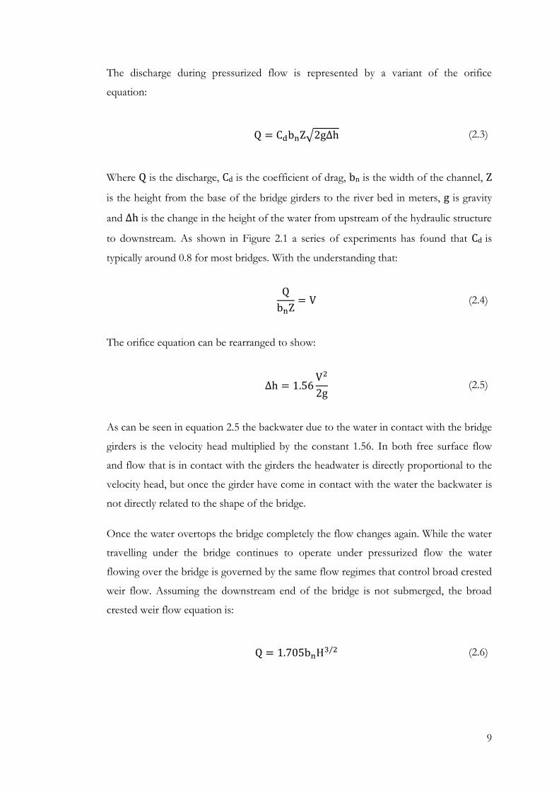
The discharge during pressurized flow is represented by a variant of the orifice

equation:

√ (2.3)

Where Q is the discharge, Cd is the coefficient of drag, bn is the width of the channel, Z

is the height from the base of the bridge girders to the river bed in meters, g is gravity

and Δ is the change in the height of the water from upstream of the hydraulic structure

to downstream. As shown in Figure 2.1 a series of experiments has found that Cd is

typically around 0.8 for most bridges. With the understanding that:

(2.4)

The orifice equation can be rearranged to show:

(2.5)

As can be seen in equation 2.5 the backwater due to the water in contact with the bridge

girders is the velocity head multiplied by the constant 1.56. In both free surface flow

and flow that is in contact with the girders the headwater is directly proportional to the

velocity head, but once the girder have come in contact with the water the backwater is

not directly related to the shape of the bridge.

Once the water overtops the bridge completely the flow changes again. While the water

travelling under the bridge continues to operate under pressurized flow the water

flowing over the bridge is governed by the same flow regimes that control broad crested

weir flow. Assuming the downstream end of the bridge is not submerged, the broad

crested weir flow equation is:

(2.6)

10

Where:

(2.7)

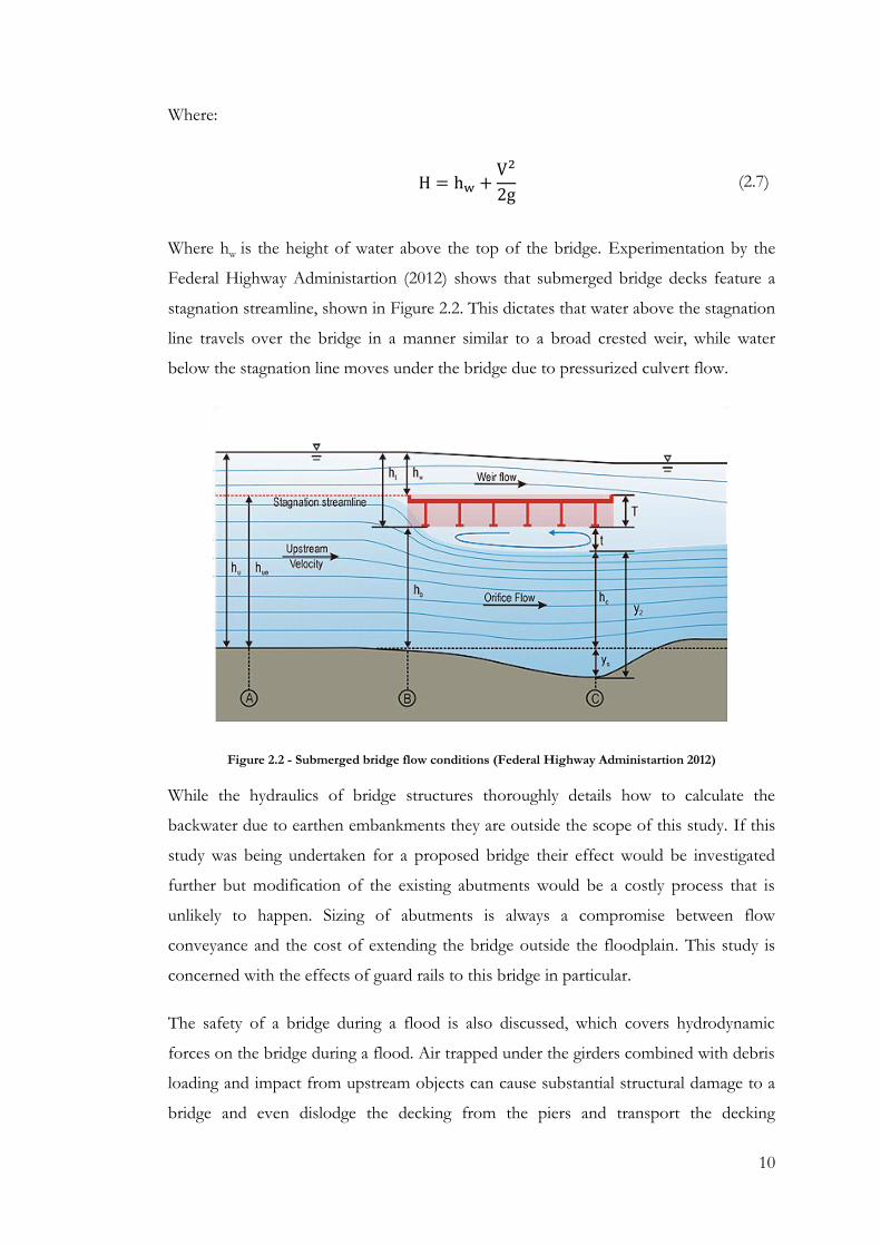
Where hw is the height of water above the top of the bridge. Experimentation by the

Federal Highway Administartion (2012) shows that submerged bridge decks feature a

stagnation streamline, shown in Figure 2.2. This dictates that water above the stagnation

line travels over the bridge in a manner similar to a broad crested weir, while water

below the stagnation line moves under the bridge due to pressurized culvert flow.

Figure 2.2 - Submerged bridge flow conditions (Federal Highway Administartion 2012)

While the hydraulics of bridge structures thoroughly details how to calculate the

backwater due to earthen embankments they are outside the scope of this study. If this

study was being undertaken for a proposed bridge their effect would be investigated

further but modification of the existing abutments would be a costly process that is

unlikely to happen. Sizing of abutments is always a compromise between flow

conveyance and the cost of extending the bridge outside the floodplain. This study is

concerned with the effects of guard rails to this bridge in particular.

The safety of a bridge during a flood is also discussed, which covers hydrodynamic

forces on the bridge during a flood. Air trapped under the girders combined with debris

loading and impact from upstream objects can cause substantial structural damage to a

bridge and even dislodge the decking from the piers and transport the decking

11

downstream. A similar event happened in Warwick to the McCahon Bridge just

downstream of the O.O. Madsen when it was hit by a shipping container in the 2013

floods. Since the O.O. Madsen Bridge has survived several large flood events which

have overtopped the deck, the safety of the forces on the bridge was considered outside

the scope of the study.

2.2 1D/2D Flood Models

Since the advent of computers flood modelling has become a more exact and accessible

science. Today there are a multitude of 1D and 2D flood models, with varying benefits

and limitations. Some notable examples are:

HEC-RAS – Stands for Hydraulic Engineer Centre River Analysis System, and

is published by the US Army Corps of Engineers (2014). HEC-RAS is a free 1D

flood model useful for modelling rivers within their banks, open channels or

other waterways where the flow can be considered essentially one dimensional.

Colloquially considered as the bench-mark of 1D flood models.

TUFLOW – The model used by SKM to undertake the Condamine River flood

study. Created by BMT WBM, it is covered extensively later in this report.

MIKE Flood – Incorporates several 1D and 2D programs within a single

package to model various combinations of flows, including rivers, floodplains,

coastal (including tidal incursion).

XP Solutions models – Includes XPSWMM, XPStorm, XP2D and other

applications for a complete flood modelling package. XPSWMM is included in

TUFLOW to model the 1D elements.

1-Dimensional flood models are useful for modelling rivers within their banks, culverts,

stormwater pipes or other flow patterns that are mostly 1-Dimensional when viewed

topographically (Syme 2011). 1D flood models use a series of cross sections to simulate

the depth and flow of water through the 1D line representing the flow object. While

they may sound limited in application, their low computation times make them a

practical alternative to 2D flood models when the flow can be represented 1

dimensionally accurately.

12

According to the Hydraulic Guidelines for Bridge Design Projects (DTMR 2013), if the

flow regime stays within the banks of the river, the hydraulic design of the bridge can be

estimated with a 1D model such as HEC-RAS, but if the river breaks its banks and

moves into the surrounding flood plain the behaviour no longer conforms to the

assumptions of a 1D model and a 2D approach must be employed. Flooding of the

Condamine River frequently leads to the river bursting its banks and flow proceeds into

the flood plain, requiring the use of a 2D flood model.

Most 1-D flood models operate under simple open channel flow equations, however 2-

Dimensional flood models use and finite difference methods are used to calculate the

depth averaged free surfaced flow in grid elements as opposed to a single line. The

more complex equations allow the models to include factors such as inertia and

momentum (Syme 2011) which a 1-D model does not account for. This document will

cover 2D flood modelling as it relates to the software package TUFLOW, because it is

the program that was used for the Condamine River Flood Study, and because

TUFLOW is one of the more popular 2D flood models used within Australia and the

UK (Pender 2009). A comparison and discussion into the assumptions, applications and

limitations of different 2D flood engines could form a project in its own right. From the

TUFLOW manual, “TUFLOW is a computer program for simulating depth-averaged,

two and one-dimensional free-surface flows such as occurs from floods and tides.”

(WBM 2007).

2D flood models require accurate topographical data in order to model the flows

effectively. This is usually accomplished using laser imagery from aircraft. Calibration of

2D models generally involves changing the Roughness values for the channel and flow

plain until the model conforms to historical flood data.

The main limitation for a 2D model is the computation time required to solve the

model. The author of TUFLOW, Bill Syme (2011) comments that “Cell sizes should be

large enough to minimise run-times, but small enough to meet hydraulic objectives”.

This means the mesh size for a 2D flood model can be up to 15m per grid, even in

urban areas. At that resolution many hydraulic objects such as culverts ca not be easily

modelled. TUFLOW is powerful because it is interlinked with the 1D model XP-

SWMM. Within a single 2D TUFLOW model many elements can be modelled as 1D

objects and the flows from the two models will interact and affect each other. This

13

means that objects that would otherwise be too small to model effectively using the grid

can be easily placed in the model to improve accuracy.

Figure 2.3 - 1D/2D model velocity contours (B.C. Phillips 2005)

Figure 2.4 - 2D only model velocity contours (B.C. Phillips 2005)

14

Figure 2.3 and Figure 2.4 show a comparison of a flood plain modelled with a 1D/2D

model compared to a pure 2D model. The study compared both results to actual data

obtained from river depth gauges and flood extent surveys and found that a 1D/2D

combined model produced significantly more accurate results than a pure 1D or pure

2D model. They claimed that the results of the 2D model could have been made more

accurate by decreasing the size of the 2D mesh, but this would significantly increase the

processing time. It was concluded “that these comparisons highlighted the advantages

of being able to define narrow watercourses and crossing using 1D elements and to link

these to a 2D floodplain.” (B.C. Phillips 2005) For this reason, the majority of flood

models created today are a combination 1D/2D model.

2.2.1 Modelling Bridges in a 2D Flood Model

Within 1D/2D flood modelling there are multiple methods of modelling bridge piers

and the bridge deck once it become inundated.

The first method is modelling the bridge piers as raised structures. This is

achieved by taking the elements that the bridge piers occur on and increasing

the elevation so they match the bridge height in reality. This has the advantage

of being very simple and easy to implement, but may not be accurate for several

reasons. Ordinarily, bridge piers in reality are not square edged objects because

of the poor hydrodynamic performance exhibited by such a structure. The

bridge piers may also not line up with the mesh of the 2D model at all. The

flow exhibited around a blocked out cell often does not match precisely with

reality. The coarseness of most 2D meshes means that often not all the energy

losses experienced from the increased velocities and eddy currents are correctly

accounted for.

In TUFLOW a flow constriction can be set to limit the flow of water through

the grid. This means a single square can be set to reduce the flow by 75%, which

could be very accurate if the bridge pier only takes up the space of 75% of the

block. Due to the inertial component of the equation used by TUFLOW this

often leads to a much more accurate result than increasing the height of the

element.

The elements that the bridge piers are drawn on can have the Manning’s n

roughness coefficient increased to increase the friction in the element. Similar to

a flow constriction this acts as a momentum sink. This method eliminates the

15

eddy currents experienced around the piers, which can make it useful for

modelling objects which are not as square as the 2D mesh.

Another method is to create a 1D line the width of the river with a flow

constriction equal to the ratio of the width of the piers to the width of the river.

This has the disadvantage that it may not be accurate at all flow heights, which is

important when the flood is increasing or receding.

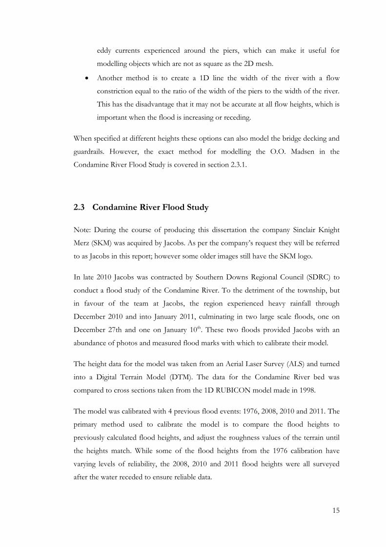
When specified at different heights these options can also model the bridge decking and

guardrails. However, the exact method for modelling the O.O. Madsen in the

Condamine River Flood Study is covered in section 2.3.1.

2.3 Condamine River Flood Study

Note: During the course of producing this dissertation the company Sinclair Knight

Merz (SKM) was acquired by Jacobs. As per the company’s request they will be referred

to as Jacobs in this report; however some older images still have the SKM logo.

In late 2010 Jacobs was contracted by Southern Downs Regional Council (SDRC) to

conduct a flood study of the Condamine River. To the detriment of the township, but

in favour of the team at Jacobs, the region experienced heavy rainfall through

December 2010 and into January 2011, culminating in two large scale floods, one on

December 27th and one on January 10th. These two floods provided Jacobs with an

abundance of photos and measured flood marks with which to calibrate their model.

The height data for the model was taken from an Aerial Laser Survey (ALS) and turned

into a Digital Terrain Model (DTM). The data for the Condamine River bed was

compared to cross sections taken from the 1D RUBICON model made in 1998.

The model was calibrated with 4 previous flood events: 1976, 2008, 2010 and 2011. The

primary method used to calibrate the model is to compare the flood heights to

previously calculated flood heights, and adjust the roughness values of the terrain until

the heights match. While some of the flood heights from the 1976 calibration have

varying levels of reliability, the 2008, 2010 and 2011 flood heights were all surveyed

after the water receded to ensure reliable data.

16

Figure 2.5 - Calibration flood heights around Warwick

Figure 2.5 shows that the flood heights obtained by the model are reasonably accurate,

with the majority of the flood points within 0.2m of the actual value.

Along with numerical validation, several community consultation sessions were held

with the help of Southern Downs Regional Council. These sessions encouraged local

citizens to bring along photographs and comment on the extents of the flood from

memory compared to the predictions made by the flood model. This proved to be

invaluable for the Leyburn model, as they identified that the model did not behave as

the 1976 flood did. Further analysis revealed a road that did not exist back then was

making an artificial levee in the current model redirecting flow.

2.3.1 Modelling the O.O. Madsen in TUFLOW

When modelling the O.O. Madsen Bridge, SKM first attempted to use a 1D flow

constriction modelled to the height of the bridge. This did not produce accurate results,

and consultation with the locals showed that the flow extents upstream of the bridge

were quite different to what the model was predicting. Jacobs then remodelled the

bridge as a series of 2D flow constrictions on top of one another. The layout of the

flow constrictions is shown in Figure 2.6.

17

Figure 2.6 - O.O. Madsen Bridge flow constriction in TUFLOW

TUFLOW calculates the depths and velocities at the centre of the grids as opposed to

the nodes. Water in TUFLOW cannot travel diagonally, only perpendicular to the edges

of each grid. In order for the water to flow from one grid into the grid diagonally

adjacent the program calculates the flow going across two lots of lines. In Figure 2.6 the

triangles represent the edges where the flow constriction occurs.

The flow constriction was created in 3 layers. The first layer represented the area under

the bridge deck, where the only flow constriction was the bridge piers. TUFLOW

calculates the flow constrictions based on the equations presented in Hydraulics of

Bridge Waterways (Bradley 1978). The energy loss coefficient for the bridge piers is set

to 0.2. The consultants explained that 0.2 was a higher than normal setting, but the

model was not producing accurate results with lower coefficients. Then within the

program the obvert (lowest portion of the bridge girders, or highest point of the flow

opening) is specified. A blockage of 5% was also applied to the bridge pier layer to

more accurately replicate the flow.

18

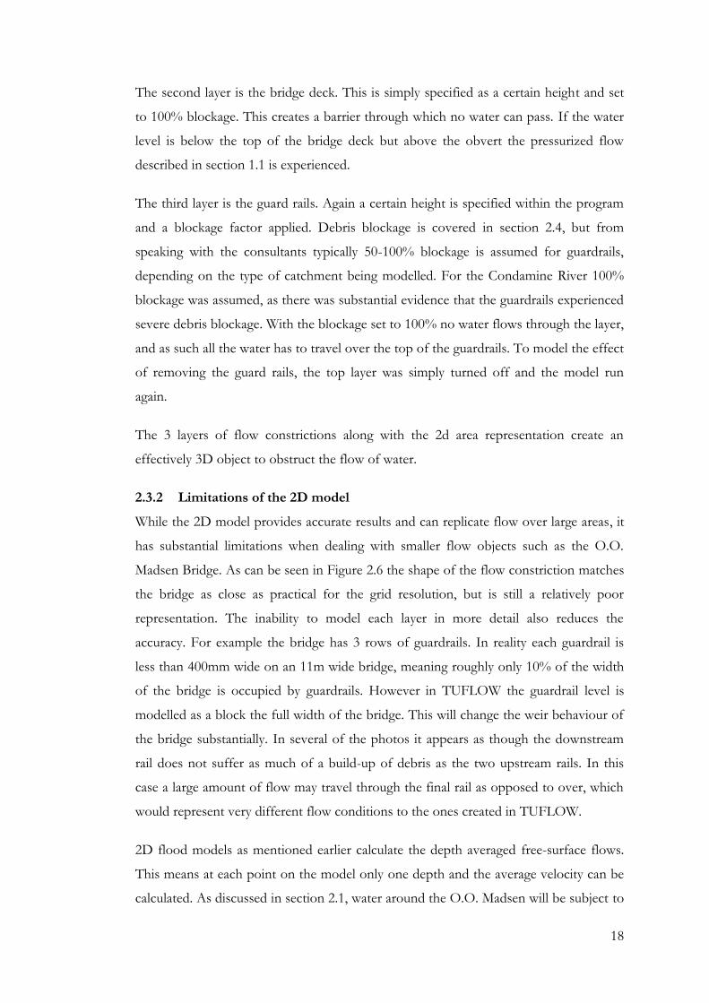
The second layer is the bridge deck. This is simply specified as a certain height and set

to 100% blockage. This creates a barrier through which no water can pass. If the water

level is below the top of the bridge deck but above the obvert the pressurized flow

described in section 1.1 is experienced.

The third layer is the guard rails. Again a certain height is specified within the program

and a blockage factor applied. Debris blockage is covered in section 2.4, but from

speaking with the consultants typically 50-100% blockage is assumed for guardrails,

depending on the type of catchment being modelled. For the Condamine River 100%

blockage was assumed, as there was substantial evidence that the guardrails experienced

severe debris blockage. With the blockage set to 100% no water flows through the layer,

and as such all the water has to travel over the top of the guardrails. To model the effect

of removing the guard rails, the top layer was simply turned off and the model run

again.

The 3 layers of flow constrictions along with the 2d area representation create an

effectively 3D object to obstruct the flow of water.

2.3.2 Limitations of the 2D model

While the 2D model provides accurate results and can replicate flow over large areas, it

has substantial limitations when dealing with smaller flow objects such as the O.O.

Madsen Bridge. As can be seen in Figure 2.6 the shape of the flow constriction matches

the bridge as close as practical for the grid resolution, but is still a relatively poor

representation. The inability to model each layer in more detail also reduces the

accuracy. For example the bridge has 3 rows of guardrails. In reality each guardrail is

less than 400mm wide on an 11m wide bridge, meaning roughly only 10% of the width

of the bridge is occupied by guardrails. However in TUFLOW the guardrail level is

modelled as a block the full width of the bridge. This will change the weir behaviour of

the bridge substantially. In several of the photos it appears as though the downstream

rail does not suffer as much of a build-up of debris as the two upstream rails. In this

case a large amount of flow may travel through the final rail as opposed to over, which

would represent very different flow conditions to the ones created in TUFLOW.

2D flood models as mentioned earlier calculate the depth averaged free-surface flows.

This means at each point on the model only one depth and the average velocity can be

calculated. As discussed in section 2.1, water around the O.O. Madsen will be subject to

19

culvert flow, weir flow and some of the water will stagnate around areas where flow is

minimal such as behind the piers or in between guard rails. This also means the depth is

only known at the centre of 15m grids, and the accuracy of the depth of the water

would be a function of the size of the grid.

One of the other major problems is that the model has been calibrated to fit a flood

event over a large area as well as possible, and the calibration does not necessarily

reproduce every small aspect of the flood accurately. For example, while the model has

a good overall fit to the surveyed flood heights in the calibration floods, there are not

many calibration points near the O.O Madsen, with only 2 near the bridge upstream

and none downstream for a considerable distance. In the 2011 event the flood heights

in front of the bridge are represented very accurately, with around 0.1m error. However

in the 2010 calibration event, only 2 weeks prior, the modelled flood height immediately

upstream of the bridge is 0.5m higher than the surveyed flood height. The Jacobs report

claim that a head loss of up to 0.5m was experienced in a 1 in 100 AEP flood, but the

model experienced an error of the same magnitude in one of the successful calibration

runs.

When asked as to how the head loss over the bridge was calibrated, it was explained

that the bridge was modelled and briefly modified to replicate the calibration flood

heights. The micro was modified to reflect the macro, and this does not mean that the

micro is still accurate.

Additionally, the accuracy of the DTM used for the 2D flood model is unknown. DTM

models give an elevation at a spatial coordinate, normally over a rectangular grid. This

means the accuracy of the height data is again a function of the size of the grid, but the

size of the grid and the nature of this function was not found through the course of the

literature review.

2.3.3 Removal of Guard Rails from the O.O. Madsen

Part of the study involved investigating options for reducing the damage caused by

floods. Under consultation with the local population it was determined that the guard

rails becoming congested with debris could be leading to increased flood depths

upstream from the bridge.

20

Figure 2.7 - 100 year ARI flood depths (Jacobs 2012)

Figure 2.8 - 100 year ARI extents after removal of O.O. Madsen guardrails (Jacobs 2012)

21

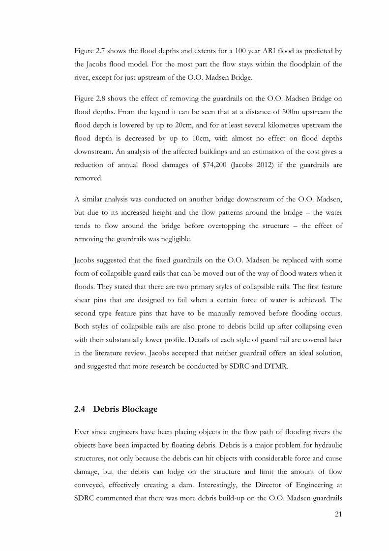
Figure 2.7 shows the flood depths and extents for a 100 year ARI flood as predicted by

the Jacobs flood model. For the most part the flow stays within the floodplain of the

river, except for just upstream of the O.O. Madsen Bridge.

Figure 2.8 shows the effect of removing the guardrails on the O.O. Madsen Bridge on

flood depths. From the legend it can be seen that at a distance of 500m upstream the

flood depth is lowered by up to 20cm, and for at least several kilometres upstream the

flood depth is decreased by up to 10cm, with almost no effect on flood depths

downstream. An analysis of the affected buildings and an estimation of the cost gives a

reduction of annual flood damages of $74,200 (Jacobs 2012) if the guardrails are

removed.

A similar analysis was conducted on another bridge downstream of the O.O. Madsen,

but due to its increased height and the flow patterns around the bridge – the water

tends to flow around the bridge before overtopping the structure – the effect of

removing the guardrails was negligible.

Jacobs suggested that the fixed guardrails on the O.O. Madsen be replaced with some

form of collapsible guard rails that can be moved out of the way of flood waters when it

floods. They stated that there are two primary styles of collapsible rails. The first feature

shear pins that are designed to fail when a certain force of water is achieved. The

second type feature pins that have to be manually removed before flooding occurs.

Both styles of collapsible rails are also prone to debris build up after collapsing even

with their substantially lower profile. Details of each style of guard rail are covered later

in the literature review. Jacobs accepted that neither guardrail offers an ideal solution,

and suggested that more research be conducted by SDRC and DTMR.

2.4 Debris Blockage

Ever since engineers have been placing objects in the flow path of flooding rivers the

objects have been impacted by floating debris. Debris is a major problem for hydraulic

structures, not only because the debris can hit objects with considerable force and cause

damage, but the debris can lodge on the structure and limit the amount of flow

conveyed, effectively creating a dam. Interestingly, the Director of Engineering at

SDRC commented that there was more debris build-up on the O.O. Madsen guardrails

22

in the January 10 2011 flood, only 2 weeks after the December 27 2010 flood. While the

literature review offered no certain explanation, one suggestion from a local engineer

was potentially more rainfall in different parts of the catchment where the debris was

not washed away by the first flood.

Figure 2.9 - Debris blockage on the O.O. Madsen after the 2011 floods (Warwick Daily News, 2011)

Whilst there has been some study regarding the blockage of smaller flow objects, such

as culverts and stormwater drainage inlets, the blockage of larger objects is generally

considered on a case by case basis. Section 11 of the most recent review of Australian

Rainfall and Runoff (Weeks et al. 2013) was devoted to the effects of blockage on

hydraulic structures. The text explains that there is still much debate amongst experts as

to what design debris blockages of structures should be assumed. A number of studies

were done around Wollongong during the flooding in 1998, but much of the data

gathered is specific for the catchments with similar characteristics to the Wollongong

area (Weeks et al. 2013). AR&R confirms that there is still a lot of work to be done in

this field.

23

The document does however offer some interim recommendations for assumed design

debris blockages for some structures, as well as some general comments for bridges. It

recommends assuming a 100% blockage of handrails and traffic barriers for a severe

blockage case. Different values are specified depending on the height of the bridge and

the distance between the piers. At its highest point the opening of the O.O. Madsen is

roughly 5.5m tall, however the abutments are grass banks at shallow angles, and as such

the height of the bridge decreases gradually to zero. AR&R provides a foot note stating

that the degree of blockage should be estimated based on the probability of groupings

of debris - known as debris rafts - from upstream. The bridge piers are roughly 13m

apart, and from the literature review blockage of the underneath of the structure has not

been a major issue during the past. Historically, it seems that for the O.O. Madsen that

the main concerns for flow lie with the guardrails.

Debris blockage not only leads to a decrease in hydraulic capacity but greatly increases

the force on the bridge structure. Debris Forces on Highway Bridges (Parola 2000) is a

literature review that gathered previous data collected by various sources to try and

form some generic equations to predict the effect of debris loading on piers and

roadways. The data for the investigation was gathered from two major attempts by

different universities to record the forces produced by debris loading. Both achieved

markedly different results, which further indicate that more research needs to be done

into debris blockage of structures. The report did not go into any detail about how to

predict the debris loading on guardrails. Drawings obtained from the O.O. Madsen

show that the guard rails have been changed since the bridges construction to a stronger

design to combat the effects of debris loading, as well as provide more resistance to

vehicle collisions.

2.5 Bridge Scour

Scour is defined as the movement of sediment and soil around bridge piers and

abutments by the erosive action of flowing water (TMR 2013). While investigating the

scour around the O.O. Madsen is not a primary objective of this project, scour has

implications for the conveyance of flow around a bridge during a flood.

24

Hydraulics of Bridge Waterways (Bradley 1978) briefly discusses the effect of bridge

scour on backwater. Essentially scour is due to the flow constriction created by the

bridge and its abutments. Reducing the available area to convey flow increases the

velocity; this increases shear on the stream bed which transports soil and sediment

downstream. The shifting of the soil and sediment is known as scour. While scour can

potentially occur at all times, it’s most pronounced during the increased velocities

experienced during flooding. When the water in the channel comes into contact with

the bridge girders the velocity increases further due to the pressurized culvert flow

effect.

While scouring can erode away the foundations of bridges and is one of the leading

causes of bridge failure (Wardhana & Hadipriono 2003), it has the benefit of increasing

the cross sectional area of the channel, which reduces velocities and decreases the

degree of backwater experienced. It is still not advisable to rely on scour as a means of

reducing backwater (Bradley 1978).

Scour can be difficult to measure, since the peak depth of the scour hole often occurs at

the height of the flood, and the hole can be filled by sediment as the flood recedes

(TMR 2013). In the long term it is conceivable that at some stage the transport of

sediment into the scour holes matches the transport of sediment out of the scour hole.

In this steady-state scenario the backwater would be nearly eliminated as the river has

reached is former flow regimes. However, in reality the ground below the bridge piers

would not be homogenous, and would likely contain boulders or rock strata that cannot

be moved by sediment transport. With such factors it’s unlikely that the channel will

ever achieve this soil transport steady-state.

Since the degree of scour around the O.O. Madsen Bridge is not known, it is not

possible to comment on the degree of effect scour could have on the depths upstream

of the O.O. Madsen. From the literature it is likely that a flat channel bed would

overestimate the effect of backwater if the abutments were modelled. Since only a

section of the bridge is being modelled a flat channel bed should be accurate enough to

investigate the effects of the guardrails.

25

2.6 CFD Modelling and Bridges

During the course of the literature review it became clear that there was a gap in the

literature, in that no one had used 3D CFD modelling to predict the change in depth of

a river over a bridge structure. CFD modelling has been used extensively to model the

turbulence and scour of a bridge during flooding conditions. Zhi-wen et.al (2012) found

that CFD modelling using 3D Reynolds-averaged Navier-Stokes equations (as used in

the current study) combined with the standard k-epsilon turbulence model can predict

the complicated flow around bridge piers. While their models did not accurately predict

the location of the scour holes, the mechanisms by which the scour holes were caused

were accurately represented by the CFD model.

A survey of bridge collapses in the US by F Wardhana and Hadipriono (2003) found

that over half of bridge collapses could be attributed to scouring and flood damage. In

consultation with the local engineers in Warwick and during the literature review it was

found that scouring has not been investigated around the O.O. Madsen, and could

potentially be a subject of future research.

Open channel CFD modelling has been used to study the hydrodynamic forces of an

inundated bridge deck, but not the resultant head-loss of the bridge deck being

overtopped. Kerenyi, Sofu and Guo (2009) investigated the forces of flood waters

through several shapes of bridges, in order to see the effects of using hydro-dynamically

shaped bridges in flood prone waterways. The investigation involved creating scale

models to verify the results obtained from the CFD modelling. The study also featured

a comparison between another piece of industry software, STAR-CD and Fluent.

STAR-CD and Fluent were found to each be better at modelling different behaviours of

the water over the bridge. Overall the 2 software packages were found to be good at

replicating the coefficient of drag over the bridge, but less accurate when the lifting

forces on the bridge were analysed. It was stated however that the flows were calibrated

for a single style of bridge, and while the other bridge models did not reproduce the

results as accurately, if they had been calibrated in the same way the results would have

been improved. The study concluded that while the CFD modelling did not consistently

produce accurate results, there is a lot of potential for CFD modelling to be used in the

future and with more refinements to the model accurate results could have been gained.

26

It is important to note that the study fully modelled the bridge guardrails as they would

be constructed, and did not account for the extra forces generated by debris loading.

Since the O.O. Madsen Bridge has survived several large flood events and has not

experienced any movement or major structural damage, it has been assumed that the

hydrodynamic forces on the bridge are not a concern and are outside the scope of this

study. However, the study by Kerenyi, Sofu and Guo (2009) has shown that Fluent is

relatively accurate at predicting the level of drag over the bridge, which shows Fluent

has a potential for accurately modelling the head loss caused by the O.O. Madsen.

2.7 Collapsible Guardrails

The literature review showed surprisingly little information for collapsing guard rails,

however a bridge engineer from Jacobs had worked with several cases previously and

provided information about his experience with collapsible guard rails.

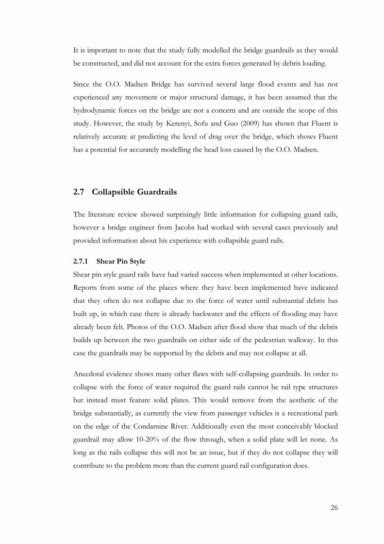
2.7.1 Shear Pin Style

Shear pin style guard rails have had varied success when implemented at other locations.

Reports from some of the places where they have been implemented have indicated

that they often do not collapse due to the force of water until substantial debris has

built up, in which case there is already backwater and the effects of flooding may have

already been felt. Photos of the O.O. Madsen after flood show that much of the debris

builds up between the two guardrails on either side of the pedestrian walkway. In this

case the guardrails may be supported by the debris and may not collapse at all.

Anecdotal evidence shows many other flaws with self-collapsing guardrails. In order to

collapse with the force of water required the guard rails cannot be rail type structures

but instead must feature solid plates. This would remove from the aesthetic of the

bridge substantially, as currently the view from passenger vehicles is a recreational park

on the edge of the Condamine River. Additionally even the most conceivably blocked

guardrail may allow 10-20% of the flow through, when a solid plate will let none. As

long as the rails collapse this will not be an issue, but if they do not collapse they will

contribute to the problem more than the current guard rail configuration does.

27

Initial prototypes were a single rail stretching the entire length of the bridge crossing.

Unfortunately these types tended to collapse in sections or not at all, rarely collapsing

the whole way over the channel. The sections left standing often held the collapsed

sections from collapsing completely. Later iterations were created in sections that could

collapse independently which led to more consistent collapses during flood events.

There is also anecdotal evidence to suggest that shear pin style guard rails have been

buckled and bent by delinquents swinging from them.

The final problem for self-collapsing guard rails is to ensure they collapse from the

forces created by flood waters but still maintain safety for the public. AS 5100 (Australia

2004) details design criteria for bridges and includes design forces for vehicle and

pedestrian guard rails.

There are 3 guardrails on the O.O. Madsen. From upstream to downstream, the first

guardrail sits between the pedestrians and the edge of the bridge, the second rail

between the pedestrians and road traffic and the third rail between road traffic and the

edge of the bridge. The first guard rail is therefore only designed for pedestrian loads,

while the second and third need to cater for loads produced from impacts by vehicles.

Clause 11.5 states that pedestrian guardrails need to be designed for a static load of

0.75kN/m at the top of the rail. Some preliminary calculations show that rails with a

0.3m tall barrier along the top could conceivably collapse when water velocities reach

1.5m/s, which are the highest velocities experienced at the O.O. Madsen Bridge during

the 100 year ARI. However this still requires the flood waters to reach the top of the rail

before it collapses, and as Figure 2.10 shows there is often substantial debris build-up

during the rising section of the flood.

28

Figure 2.10 - O.O. Madsen Bridge during 2010 Flood (Warwick Daily News, 2010)

The second guard rail on the O.O. Madsen Bridge is greater than 800mm tall and is

therefore classified as a regular height barrier as per table 11.2.3 (Australia 2004). The

third guardrail sits at 750mm and is therefore a low style guard rail (the kerb increases

their height but the standards only consider the guardrails themselves). Table 11.2.2

(Australia 2004) dictates the ultimate loads that the guardrails are required to resist, and

give values for outward loads and inward loads. For the second guardrail the water will

be acting to push the guard rail inward toward traffic, but for the third guardrail the

water will be acting outward. For a regular height guardrail, the inward load is a

distributed force of 72.7kN/m, and for a short guardrail the outward force is

113.6kN/m. These forces are far in excess of what can be produced by water in the

Condamine River under the worst flood conditions probable. It is therefore

inconceivable that traffic barriers could be made to automatically collapse under flood

conditions.

2.7.2 Manually Collapsed Style

While it is certainly conceivable that a manually collapsed style of guardrail could be

designed to withstand the required loads, the manual style guardrails are not without

faults either. This style of guard requires that the roads be closed before the guardrails

are lowered, which can place employee’s at risk in the event of a quickly approaching

flood. In order to remove the pins before an event that will overtop the bridge, effective

flood warning capabilities have to be in place in order to foresee a flood and lower the

guardrails before the flood arrives.

29

Currently predicting floods in Australia is difficult, as the majority of catchments in

Australia simply do not have enough long term data to create accurate trends.

Additionally, many catchments do not have rainfall gauges in every reach of a

catchment, meaning the available data may under or over predict a flood due to the

difference in rainfall temporal patterns. In the case of a false prediction, an unnecessary

road closure can aggravate the local people and lead to a reduced faith in the abilities of

the flood engineers. However, SDRC has invested into flood warning capabilities for

Killarney, a town upstream of Warwick on the Condamine River. Previous floods have

shown that flood heights at Killarney are achieved in Warwick roughly 24 hours later. In

this case manually collapsible style guardrails could be implemented with a reasonable

amount of faith in the bridge being closed appropriately.

30

Chapter 3

Methodology

Chapter 3 details the methodology used to solve the problem of water flowing over the

O.O. Madsen Bridge. Generating an accurate CFD simulation requires several steps.

Firstly the geometry for the model must be created. The geometry includes the object to

be modelled and a domain for the fluid that travels around the object. The domain is

then subdivided into finite volumes through meshing. Once the meshing has been

complete, a grid independence survey should be conducted. A grid independence survey

ensures that the resolution of the mesh is not affecting the outcome of the model. The

boundary conditions and solving options are set and the equations are solved.

The output of the model would then be validated by an experiment. While CFD

calculations are robust, they are still approximations of reality and are subject to

limitations. Validation allows the user to see if the model is accurate enough for the

required purposes.

3.1 Input Data and Assumptions

The input data for the CFD model was mostly gathered from the 2D flood model

produced by Jacobs. However, in order to get the data into a usable form for Fluent

several assumptions had to be made. For the analysis presented in this report the only

flood data modelled was the 100 year ARI flood.

The O.O. Madsen Bridge is located on a gradual bend in the Condamine River. When

water changes direction inertia that causes the water to loose energy and velocity, and in

extreme cases it can cause the surface of the water to become uneven due to the effect

of centrifugal force.

31

Figure 3.1 - Velocity vectors over O.O. Madsen

Figure 3.1 shows the velocity vectors extracted from the 2D Jacobs model. While this

shows there is a bend in the river, it is assumed that the change in direction experienced

over the bridge is insignificant, and modelling the flow in a straight line will be

sufficiently accurate for examining the effects of the guard rails.

While discharge data was available, the open channel flow option in Fluent only requires

that the depth and velocity be specified. As such the depth and velocity were extracted

in various sections through the model, shown in Figure 3.2. These sections were chosen

in order to compare the depths and velocities of the two models are varying distances

up and downstream from the bridge and at different locations along the bridge. A single

profile was taken along the tallest section of the bridge in order to create a profile of the

water as it travelled over the bridge. The input velocities and depths were taken from

the upstream boundary profile, as these values were less affected by the backwater

produced by the bridge. Data that was completely unaffected by the backwater caused

by the bridge was not attainable, because the backwater reached the boundary of the

model around Warwick, and because the model run where the bridge was removed was

not available. The final velocity was 1.5m/s, and a depth of 7m was taken.

32

Figure 3.2 - Depth and velocity sections from 2D flood model

During interrogation of the channel bed data it became apparent that there was a dip in

the profile of the bed around the location of the bridge, shown in Figure 3.3. This dip is

roughly 0.6m deep at its deepest point, and judging from the location it may have been

created as the result of scour from the turbulent flows around the bridge.

As mentioned in section 2.3 the data for the channel bed was taken from 2 sources, the

ALS data from early 2010 and cross section data from a 1D RUBICON model from

1998. Since these dates there have been 3 major flood events; 27/12/2010, 10/1/2011,

and 26/1/2013. It is conceivable that this data is no longer accurate and as such, it is

assumed that the channel of the bed is flat around the bridge. As discussed in section

2.5 a flat channel bed will likely provide a reasonable estimate of the backwater. From

Figure 3.3 and the discussion in the Condamine River Flood Study, the drop in depth of

the water over the bridge is roughly 0.5m.

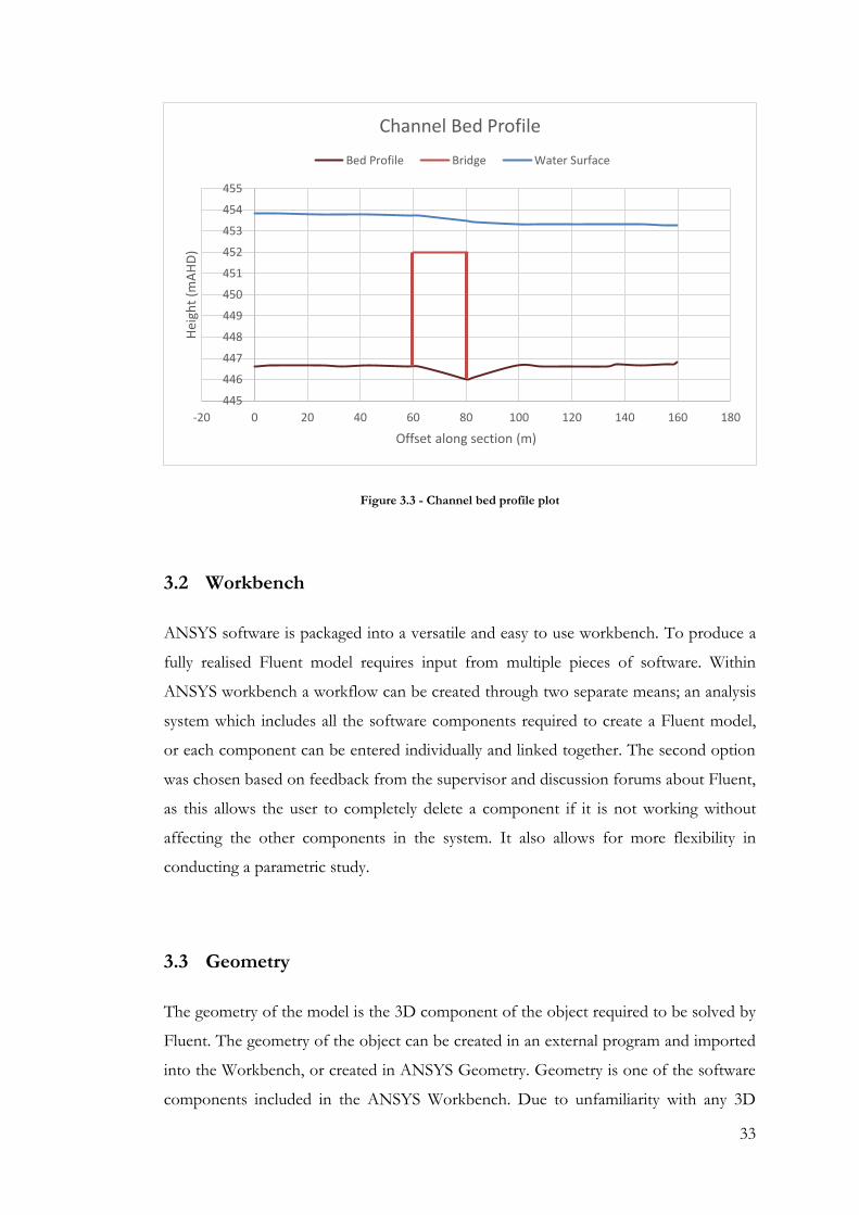
33

Figure 3.3 - Channel bed profile plot

3.2 Workbench

ANSYS software is packaged into a versatile and easy to use workbench. To produce a

fully realised Fluent model requires input from multiple pieces of software. Within

ANSYS workbench a workflow can be created through two separate means; an analysis

system which includes all the software components required to create a Fluent model,

or each component can be entered individually and linked together. The second option

was chosen based on feedback from the supervisor and discussion forums about Fluent,

as this allows the user to completely delete a component if it is not working without

affecting the other components in the system. It also allows for more flexibility in

conducting a parametric study.

3.3 Geometry

The geometry of the model is the 3D component of the object required to be solved by

Fluent. The geometry of the object can be created in an external program and imported

into the Workbench, or created in ANSYS Geometry. Geometry is one of the software

components included in the ANSYS Workbench. Due to unfamiliarity with any 3D

445

446

447

448

449

450

451

452

453

454

455

-20 0 20 40 60 80 100 120 140 160 180

Hei

ght

(mA

HD

)

Offset along section (m)

Channel Bed Profile

Bed Profile Bridge Water Surface

34

modelling software, the author decided to use ANSYS Geometry, as it was the simplest

to integrate into the Fluent workflow, and easiest to modify for subsequent model runs.

The preliminary geometry modelled was a simple cylinder representing a pier, created in

order to become familiar with the program and to find the correct boundary conditions

to predict open channel flow.

Due to restrictions in the element count for the academic licence, and the time required

to conduct a simulation the model of the bridge had to be simplified wherever possible.

Firstly, this meant that the entire length of the bridge could not be modelled. Instead, a

section of the bridge was modelled as demonstrated in Figure 3.4.

Figure 3.4 - Example of bridge section

The 3 styles of guard rails were modelled as rectangular prisms, since modelling every

tubular rail component would have taken too many elements. This was considered to be

a good approximation since the rails are generally heavily blocked by debris in severe

floods, which in terms of flow would give a similar result. The guard rails were

modelled separate to the bridge geometry in order to effectively turn them off and on

by changing their section from solid to fluid.

The I-beam girders below the bridge deck were modelled as I-beams, but this produced

errors in the mesh unless a fine mesh smoothing was specified, which created too many

elements. For the final geometry the I-beams were simplified into rectangular prisms, as

it was assumed that the flow patterns under the bridge deck would not be affected

much by the simplification.

The final bridge geometry is presented in Figure 3.5 and Figure 3.6. The right hand side

of the image is the upstream side of the bridge. The bridge decking is skewed with

respect to the flow of the river by 20°.

35

Figure 3.5 - Final bridge geometry – with rails

Figure 3.6 - Final bridge geometry - no rails

The second component of the geometry is the fluid domain. The domain gives the

extents that the fluid can occupy. An enclosure is made around the bridge for the fluid

to travel through. The geometry for the bridge is then subtracted from the enclosure,

shown in Figure 3.7. Upstream is again the right hand side of the image.

36

Figure 3.7 - Geometry of fluid enclosure

The domain extends for a large distance upstream and downstream of the bridge in

order to minimise the effects of the boundary conditions on the flow around the bridge.

While there was no indication from the literature review of distances required for two-

phase CFD calculations, aerodynamic simulations have found that roughly 3 body

lengths in front and 5 body lengths behind are a minimum to prevent interference from

boundary conditions (Lanfrit 2005). Since measuring backwater was the main objective

of the model, it was required that the effect of the inlet boundary be minimised as much

as possible. As such the model was given roughly 4 body lengths up and downstream

for the domain.

3.4 Meshing

Meshing is regarded as one of the most important steps in CFD modelling. Fluent uses

finite volume methods to solve the various equations at each point or node of the

model. If these elements are too few or not close enough to accurately calculate the

gradients for the partial differential equations the model will not converge on the

correct answer, particularly in points of complex flow. Thus the mesh has to be

sufficiently fine to calculate the correct result, but not wasteful. Excess nodes increase

calculation time. In areas of simple flow may add nothing to the accuracy of the model.

While there exists a lot of studies and information for creating a mesh intended for

aerodynamics around car bodies, there was no literature available that has explored the

ideal options for open channel flow.

37

In order to check that the mesh is accurately solving the problem a grid independence

study would be conducted. A grid independence survey is essentially a sensitivity

analysis of the mesh performed by altering various parameters and seeing their effect on

the model. The parameters are altered until the result stops changing, in which case the

user can be certain that the solution of the model is not being affected by the resolution

of the mesh. Due to the run times of the model a grid independence study was not

possible.

The mesh can be optimised automatically by ANSYS meshing for different styles of

numerical solvers. In this case this physics preference is set to CFD, since the mesh is

being used to solve a fluid problem. Similarly, the solver preference is set to Fluent.

Given the geometry of the O.O. Madsen Bridge a regular tetrahedral mesh was used

with a coarse Relevance Centre and Medium Smoothing. A medium relevance centre

was trialled but due to the size of the domain the node count became prohibitive.

Instead Body Sizing functions were employed. A body sizing function allows the user to

specify a maximum element size for the domain with a separate geometry dictating the

boundary of the sizing function. The body sizing function around the bridge is shown

as a green box in Figure 3.8.

Figure 3.8 - Body sizing function

ANSYS Meshing offers several types of advanced sizing functions. After experimenting

with all 5 functions, the Proximity and Curvature advanced sizing function was

specified. It gave the most uniform and smooth mesh, and allows for control over the

curvature normal angle and the accuracy of the proximity.

38

The growth rate controls the rate of increase in the size of the elements. A growth rate

of 1.2 means each element can only be 20% larger than any of the elements around it.

Initially a growth rate of 20% was used on the preliminary cylindrical pier model, but a

greater convergence was found with a 10% growth rate. Figure 3.9 shows the effect of

the growth rate, with the fine mesh around the surface of the water gradually increasing

in size to the top of the domain.

Figure 3.9 - View of entire meshed domain

Based on the findings of Lanfrit (2005) the mesh was given a program controlled

automatic inflation, set to first aspect ratio, with a maximum of 5 layers and 20%

growth rate. This allowed the model to converge however the need for the first aspect

ratio inflation was overcome in the final version of the mesh with the body sizing

function placed around the bridge, and a face sizing function was created for the faces

of the bridge, limiting the maximum cell size to 0.005m. The face sizing function had

that added benefit of giving a higher resolution to the sides of the pier where there was

a substantial amount of turbulence. The final mesh had 1.35 million nodes and 7.5

million elements. A cross section of the final mesh aroung the bridge and pier is shown

in Figure 3.10.

39

Figure 3.10 - Cross sectional view of mesh

3.5 Fluent

Fluent is one of the two CFD solvers included in the ANSYS package, with CFX being

the other. While either component could have been used to model the O.O. Madsen,

the popularity within the literature, combined with the supervisor’s previous experience

led to Fluent being chosen.

3.5.1 General Set Up

Two solver types are presented, pressure-based and density-based. Since the backwater

caused by the bridge leads to a head loss over the top the pressure-based solver was

selected. The velocity formulation was left at the default Absolute, and gravity was

enabled as 9.81m/s downwards.

All the literature concerning open channel flow always considered the flow as transient.

Attempts to solve open channel flow in a steady state resulted in a model that

immediately diverged. The ANSYS documentation mentioned that smaller step sizes are

preferable initially in order to get the model to converge. Once the model has

converged the step size can be made larger to quickly develop the required flow

patterns. Before the first convergence the time step was set to 0.01 seconds. The time

step was adjusted throughout the modelling process to try and optimise the iterations

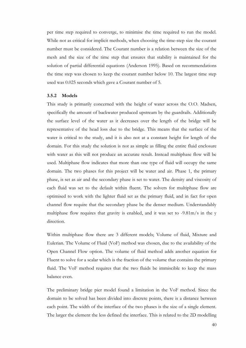
40

per time step required to converge, to minimise the time required to run the model.

While not as critical for implicit methods, when choosing the time-step size the courant

number must be considered. The Courant number is a relation between the size of the

mesh and the size of the time step that ensures that stability is maintained for the

solution of partial differential equations (Anderson 1995). Based on recommendations

the time step was chosen to keep the courant number below 10. The largest time step

used was 0.025 seconds which gave a Courant number of 5.

3.5.2 Models

This study is primarily concerned with the height of water across the O.O. Madsen,

specifically the amount of backwater produced upstream by the guardrails. Additionally

the surface level of the water as it decreases over the length of the bridge will be

representative of the head loss due to the bridge. This means that the surface of the

water is critical to the study, and it is also not at a constant height for length of the

domain. For this study the solution is not as simple as filling the entire fluid enclosure

with water as this will not produce an accurate result. Instead multiphase flow will be

used. Multiphase flow indicates that more than one type of fluid will occupy the same

domain. The two phases for this project will be water and air. Phase 1, the primary

phase, is set as air and the secondary phase is set to water. The density and viscosity of

each fluid was set to the default within fluent. The solvers for multiphase flow are

optimised to work with the lighter fluid set as the primary fluid, and in fact for open

channel flow require that the secondary phase be the denser medium. Understandably

multiphase flow requires that gravity is enabled, and it was set to -9.81m/s in the y

direction.

Within multiphase flow there are 3 different models; Volume of fluid, Mixture and

Eulerian. The Volume of Fluid (VoF) method was chosen, due to the availability of the

Open Channel Flow option. The volume of fluid method adds another equation for

Fluent to solve for a scalar which is the fraction of the volume that contains the primary

fluid. The VoF method requires that the two fluids be immiscible to keep the mass

balance even.

The preliminary bridge pier model found a limitation in the VoF method. Since the

domain to be solved has been divided into discrete points, there is a distance between

each point. The width of the interface of the two phases is the size of a single element.

The larger the element the less defined the interface. This is related to the 2D modelling

41

problems mentioned earlier; the accuracy can only be a great as the size of the mesh.

Since meshing the entire domain with a fine mesh was not possible due to the node

limit and time constraints, a body sizing function was introduced into the geometry to

smooth the mesh around the interface of the two phases.

Figure 3.11 - Water surface body sizing function

For this model the max element size was specified as 0.25m, and the growth rate was set

to 10%. Ideally an element size of 0.1m would have been used, but this more than

doubled the number of elements in the model which would have made computation

times completely prohibitive.

Within the VoF method the Open-Channel Flow option was enabled. The boundary

conditions for the open channel method assume that the free surface level is normal to

the direction of gravity, and as such no slope needs to be specified for the bed of the

channel.

Another limitation was found once the model was run for extended periods of time.

The interface between the two phases would grow larger making identification of the

precise surface level of the water extremely difficult as shown in Figure 3.12.

42

Figure 3.12 - Phase interface at 0.48s, 1.48s, 3.48s and 5.92s

Initially this was thought to be an issue with the VoF method; however results from

other research papers and industry simulations showed sharp fluid interfaces and even

the formation of bubbles with the VoF model. The problem was found to be the

solution method for the spatial discretization for Volume Fraction utilised by Fluent. At

default it is set to First Order Upwind, shown in Figure 3.13. By specifying the solution

method as the compressive slope limiter the interface is modelled sharper (ANSYS

2012). Figure 3.14 shows the effect of the compressive solution method after 14.25

seconds of simulation time. By utilising the compressive solution method the surface of

the water was able to be assumed as the middle of the interface. This is covered further

in section 3.7.

43

Figure 3.13 - Comparison of spatial discretization solution methods for volume fraction (ANSYS 2012)

Figure 3.14 - Interface with compressive spatial discretization specified; simulation time 14.25 seconds

For the majority of the solutions the viscous turbulence model with the standard k-

epsilon equation was chosen, with standard wall functions.

All other models were left off. Under materials the solid components were set to

aluminium. While the majority of the bridge is concrete, specifying a material for a solid

only gives it a density; surface roughness is specified in boundary conditions. Since the

bridge is not moving within the model the density is irrelevant.

44

3.5.3 Cell Zone Conditions

Cell zone conditions dictate what each body or object in the model is. For the

preliminary and for many of the initial models there was only body which was the fluid

domain. However when the rails were modelled as fluids there became 4 domains, the

fluid domain and one for each guard rail. This allows the guard rails to be easily turned

into fluid domains to allow the water to pass through. While this could have been

accomplished through deleting the rails in the geometry, by utilising the cell zone

conditions the mesh could be identical for both simulations. Within the cell zone

conditions for fluids a porosity can be specified. Porosity within Fluent essentially acts

as a momentum sink as the fluid moves through the porous media. Porosity was

experimented with but time constraints limited the ability to do a full parametric study

on different guardrail porosities.

For the final results run of the model the 3rd guardrail was specified as a fluid. Based on

images found in the literature review this was deemed to be the most realistic blockage

condition.

3.5.4 Boundary Conditions

Open channel flow only works with a selective set of boundary conditions.

Consultation of the user guide found that the inlet should be specified as a pressure

inlet and the outlet as a pressure outlet, as this only requires the free surface level and

velocity of the water to be specified, something that was easily attained from the Jacobs

flood model. The most problematic boundary was the top boundary above the air. The

ANSYS user guide advised that specifying this boundary as a pressure outlet can

sometimes lead to non-convergent solutions due to a pressure singularity in the corners

of the domain (ANSYS 2014). Running the simulation with the top boundary set to a

pressure outlet took much longer to lead to a convergent solution, with the air entering

through the pressure inlet on the upstream side of the domain and travelling straight

outwards through the top boundary. An identical situation was occurring at the end of

the model with air travelling in through the pressure outlet and out through the top

boundary. The top boundary was changed to solve as a pressure inlet, a mass flow inlet,

and a wall. The inlet options experienced the same errors as the pressure outlet, but to

varying degrees. For the final solution the top boundary was changed to a wall with zero

shear which essentially trapped the air in the box. Initially there was concern that this

might lead to a negative pressure zone as the water height drops over the O.O. Madsen,

45

but various runs of the model shows no difference in surface height when compared to

the models which allowed air to move freely through the top boundary.

One of the primary advantages of open channel flow is that it is not necessary to specify

complex boundary conditions at the inlet or split the enclosure into separate parts for

water and air. Under the multiphase tab in boundary conditions the open channel

option is selected, and for this project the Flow Specification Method used was Free

Surface Level and Velocity. The initial free surface level from the origin and velocity of

the second phase (water) at that boundary is specified.

For the inlet, the initial free surface level and velocity magnitude were set to the values

obtained from the Jacobs flood model, with a height of 3m (above the origin) and a

velocity of 1.5m/s. Since this model is concerned with the backwater created by the

bridge it is very important to understand how the inlet and outlet conditions control the

surface height of the water.

The ANSYS help documentation advises that the boundary conditions should be set as

close as possible to the expected outcome to limit the computation time. Based on the

data gathered from the 2D Jacobs model the outlet boundary was set to 0.5m lower

than the inlet. Initially this had the unexpected side effect that the air in the domain had

a velocity of 0m/s, while with equal inlet and outlet heights the velocity travelled along

at the same velocity that the water did. This is due to the initialisation which sets the

entire domain to the same velocity. The air can be “patched” into the program at a

velocity of 0m/s, but it was decided that air travelling at the same speed as the water

gives the greatest chance of producing a more defined water surface free of turbulence.

However, after running the program for several hundred iterations the air began to

travel backwards, entering through the outlet and exiting through the upstream inlet.

After 2000 iterations the velocity of the air began increasing quickly up to 42m/s. At

this velocity the wind shear effect was enough to create large turbulent eddies on the

surface of the water. That model was aborted, and the solution was restarted with the

outlet and inlet conditions at the same height.

The sides of the model used symmetry planes to create the effect that the bridge

continues on each side of the model. A symmetry plane in fluent is not quite the same

as a zero shear wall. A zero-shear wall has a zero gradient for the velocity normal to the

surface, while a symmetry plane has a zero gradient for all quantities normal to the

46

surface. So the fluid is free to move along the wall without losing energy, as it would if

more fluid was passing at the same velocity next to it.

The bottom boundary representing the river bed was set to a no-slip wall. A no slip wall

prohibits movement of the fluid along the boundary layer, which allows shear stress to

be induced in the fluid.

The boundary layer for the bridge was set as a no-slip wall as well, with a specified

roughness height of 0.013, 0.025 and 0.05mm. Due to the coarse mesh and size of the

object there was no discernible difference in the surface level of the water between the

different roughness heights.

Dynamic mesh options were not explored, and the reference values were left at the

default as specified by Fluent.

3.5.5 Initialisation

Initialisation is considered one of the most important aspects of creating a model with

open channel flow. Initialisation essentially gives each node in the model values that are

an appropriate starting point in order to reduce solution time and allow the model to

converge. For example, before initialisation the entire domain will be filled with the

phase 1 fluid with a velocity of 0m/s. If the simulation was started without being

initialised the water would have to flow in through the inlet and slowly fill the domain,

increasing the computation time dramatically. Among other things, initialisation allows

the user to specify a constant velocity for the whole domain, so that a large portion of

the domain will be close to correct before the program even begins solving. The

ANSYS user manual has an entry devoted to the initialisation of open channel flow. For

the problem presented, it was recommended that the initialisation be computed from

the inlet. This means the entire domain will be set to the inputs specified in the inlet

boundary conditions; for this problem that is the height and velocity of the phase two

fluid. The manual also recommended using a standard initialisation as opposed to the

hybrid initialisation. The initialisation allows the specification of a reference frame,

either Relative to Cell or absolute. The reference frame governs how each cell is

initialised. The two options available is every cell is initialised from a single absolute

value or they are initialised relative to the neighbouring cells, allowing a gradient of

velocities or other factors at the beginning of the model.

47

3.5.6 Solution

Fluent gives many options for solution methods and controls, but they were not

explored in this study. The user manual’s suggestions for open channel flow were the

default values options, and they were not changed. Under monitors the absolute criteria

for the residuals were set to 1.000e-4 to ensure sufficient convergence.

After many different versions of the model it became apparent that the fluid was not

behaving as expected. The surface of the water would rise before a flow obstruction,

fall after as would be expected, and then it would return to the height specified by the

boundary conditions. After rigorous experimentation with different boundary

conditions and other parameters, it appeared as though the flow had simply not had

enough simulation time to develop.

In order to understand why the flow needs time to develop it’s important to understand

what the model is trying to represent in reality. In essence the initialisation tells the

program that the water is travelling at a certain velocity in a domain with no

obstructions. When the model begins solving, it is in effect placing the bridge in the

path of flow instantaneously. The initial models were converging in 120 iterations, or a

simulation time of 0.075 seconds. In reality if an object was placed in the path of water

in an instant and observed for 0.075 seconds the flow would not have changed

substantially. This is especially true for an object 11m wide with water travelling at

1.5m/s. The model requires time for the flow to react to the obstruction that has been

placed in its path.

In order to get an estimate of how long the model has to be run for the residence time

has to be considered. The residence time is the amount of time taken for the fluid to

clear the extent of the domain being considered, in this case the bridge. The residence

time is given by equation 3.1:

(3.1)

Since the water is travelling at 1.5m/s, and the bridge is 11.2m wide a single residence

time is 7.47 seconds. However, due to the fact that the water is slowed substantially by

the rails and the bridge girders several residence times must be experienced. This model

was solved for a minimum of 3 residence times, or 22.5 seconds.

48

After increasing the size of the time step and drastically increasing the number of time

steps the model solves for the models began to display the types of flows that were

expected. Another problem was introduced when the flow had proceeded long enough

to become more turbulent then the short term model. The K-epsilon turbulence solver

produced accurate results with convergence in the order of 1.0e-3 consistently within 4

iterations per time step up until 7.5 seconds model time. At 7.5 seconds the model

began requiring more iterations per time step to converge. After 11 more time steps the

model began to diverge and was stopped. While the exact cause of the divergence is not

known it may have been due to a turbulent eddy current moving into a section of the

domain with a mesh resolution too high to be solved accurately by the turbulence

model.

The Transition Shear Stress Transport (SST) model was employed for future runs of the

model. This turbulent solver unifies the advantages of the most widely employed two-

equation models and is the most reliable model for fluids with flow separation (ANSYS

2011). The SST model gave a larger displacement of water over the bridge rails, and

continued to converge well after the K-epsilon model began to diverge. The Transition

SST solver continued to converge satisfactorily past 29 seconds, at which stage the

model was converging in a single iteration per time-step.

A summary of the changes made to models for the duration of this project is presented

in a non-comprehensive model log in Appendix D.

3.6 Scour Estimation

The HEC-RAS User Manual (Engineers 2014) gives several empirical equations for the

calculation of scour based on the size and shape of piers and locations of the

abutments. However, the methods outlined are quite limited, especially for the relatively

complex geometry of the O.O. Madsen Bridge. The abutments for the bridge are

located outside of the main flow channel, the bridge is skewed to the direction of flow

and located on a bend in the river.

Scour was not a primary concern of the project, but Fluent is quite capable of

estimating the shear stress on a wall due to the fluid moving past it. In order to get an

appreciation of the magnitude of scour around the O.O. Madsen Bridge, and how that

magnitude could be affected by the removal of the guard rails a preliminary estimation

49

of the size of particles that can be moved by water travelling under the bridge will be

undertaken.

The method used will be the entrainment function. The entrainment function provides

a relationship between the shear stress experienced and the particle size and density that

will be moved, assuming that the soil is cohesionless (Gillies 2013). Cohesive soils have

a bonding force that gives them resistance to erosion, but for this brief analysis

assuming that he soil is cohesionless is more conservative. Essentially the entrainment

function is a ratio of shear force to gravity force:

( ) (3.2)

Where Fs is the unit less entrainment force number, 0 is the shear stress on the bed in

Pa, s is the density of the soil particles in kg/m3, is the density of water in kg/m3, g is

acceleration due to gravity in m/s, and d is the diameter of the largest particle that is

moved by the shear stress. Fs varies with the Reynolds number experienced in the

stream, however once the water enters the rough turbulent flow zone Fs ≈ 0.056. With

the assumption that the Condamine River is in rough turbulent flow the equation can

be rearranged to solve for the diameter:

( ) (3.3)

Exact data for the soils in the channel of the Condamine River would be obtained for a

comprehensive study of scour around the O.O. Madsen Bridge, however for this

estimation the soil particle density will be assumed as 2650kg/m3. From this

relationship it can be seen that the diameter of the particle that can be moved increases

linearly with the shear stress.

3.6.1 Shear Stress In Fluent

In Fluent the magnitude of the shear stress is governed by the roughness height of the

boundary layer. The roughness height specified in Fluent is the equivalent sand grain

roughness height (ANSYS 2014). In order to gain an appreciation of the effect of the

roughness height on the shear stress experienced, the initial cylindrical bridge pier

50

geometry simulation was run with a multitude of roughness heights between 0 and

0.5m, and the maximum shear stress was recorded.

Roughness Height (m)

Max Shear Stress (Pa)

0 16

0.0002 20

0.002 50

0.02 90

0.05 95

0.5 119 Table 3.1 - Roughness height vs shear stress

When plotted with the roughness on a log scale, the relationship between shear stress

and roughness height appeared to be logarithmic. Reliable data for the roughness height

of the stream bed around the O.O. Madsen Bridge was not available. A roughness

height of 0.5m was specified for the bed to be conservative, but by undertaking a

comparison of shear stress vs. roughness the results can be easily adjusted later when

more accurate data is available.

Figure 3.15 - Roughness height vs shear stress

3.7 Post Processing of Data

In order to quantify the head loss experienced due to the O.O. Madsen Bridge the

location of the surface of the water will have to be found. The VoF method gives each

0

20

40

60

80

100

120

140

0.00001 0.0001 0.001 0.01 0.1 1

She

ar S

tre

ss (

Pa)

Roughness Height (m)

Roughness Height vs Shear Stress

51

cell a scalar of the fraction each phase experienced in the cell, called the volume

fraction. When the volume fraction for phase 1 is 0, the element is water, and when the

volume fraction is 1 the element is entirely air. Therefore the surface of the water or

interface of the two phases occurs where the volume fraction of either phase is equal to

0.5.

CFD-Post is another program included in workbench that is designed to provide easy

interpretation of the data from Fluent. Fluent calculates values for volumes at the centre

of a cell, but CFD-Post gives plots and exports data based on the value at the nodes

between cells (ANSYS 2014). To see the effect of the different centring options the

results were exported from both CFD-Post and Fluent as .csv files. The fidelity of the

fluent plot was substantially higher; however the final numerical answers stayed the

same. The comparisons are presented in Appendix G. The domain chosen for the

volume fraction data was a vertical plane running parallel to the flow in the centre of the

bridge. The data exported from CFD-Post has 4 columns; X-location, Y-location, Z-

location and volume fraction of the node. While the X-location should have been

entirely zero as the plane travelled through the origin, the largest value experienced was

5.96e-8, which to the numerical precision of the model can be taken as zero.

Interpretation of the data directly from the exported file is difficult. The mesh used is

tetrahedral and not rectangular, so the nodes are not in even grid coordinates that can

be easily graphed. Furthermore, the volume fraction information for the 2D plane is

interpolated from surrounding points in the 3D domain, shown in Figure 3.16. In order

to overcome these deficiencies the data was post processed with a MATLAB algorithm.

The MATLAB code is presented in Appendix E.

52

Figure 3.16 - Distribution of nodes in 2d plane

The script file imports the data and finds the y and z coordinates of each point. The

function then finds the distance between the output nodes and nodes within the

rectangular MATLAB array within a specified tolerance. The script uses a normal

distribution density function to assign a weighted value based on the distance between

all output nodes and the MATLAB node. This weighting is then multiplied by the

volume fraction to find the appropriate volume fraction for the MATLAB node. The

new MATLAB array is plotted to compare to the results from CFD-Post and Fluent to

ensure the algorithm is working as intended. The results are presented in Appendix G.

The second part of the algorithm reads the volume fraction data at each of the new

MATLAB nodes and interpolates between them to find the height at which the volume

fraction is 0.5. The surface plots are then visually compared to the volume fraction plots

to ensure the algorithm has worked as expected. The results are presented in Appendix

G.

The tolerance specified for weighting the exported nodes to the MATLAB nodes was

0.05m. This means the accuracy of the surface level found with the script is only

accurate to ±0.05m, on top of the accuracy of grid at ±0.125m. The surface level results

53

are therefore only accurate to ±0.130m. This will be considered the minimum limit of

confidence in the results.

Due to the various approximations in achieving the surface level plot in MATLAB there

was some ‘noise’ present. Estimating the change in the water surface by finding the

maximum and minimum values in the array would not have provided an accurate result.

Instead the depths from 1m to 35m both up and downstream from the bridge were

averaged. This distance was chosen to minimise the effect of the boundary conditions

and localised effects from the bridge. Assuming a geometrically random assignment of

nodes during the meshing process, averaging the depths could potentially increase the

confidence in the accuracy of the height of water. It is difficult to assign a numerical

value to this increase in confidence.

3.8 Model Validation

A critical step in producing a reliable CFD model is validating the outputs with

observations from experimental data (Trucano 2000). While flood height and extents

data was available around the bridge none of the points were close enough to verify the

depth results of the model. With an object as complex as the bridge the turbulence

would need to be validated as well. With no validation data the accuracy of the model

cannot be determined.

54

Chapter 4

Results and Discussion

Chapter 4 details the results gathered from the CFD model and interpretation of the

data. The model is confirmed as steady state, and then the effect of the guardrails on the

surface is investigated. Stagnant streamline and vector plots are used to discuss the

change in flow behaviour below the bridge, and the shear on the river bed is also

discussed. Finally the limitations of the current model and future work following on

from this project are discussed.

Wherever possible the plots are presented with upstream on the left, however in order

to convey the required information some images have upstream on the right and are

labelled as such.

4.1 Steady State Analysis

In order to interpret the data it was required that the model reach a steady state. While

fluent cannot solve open channel flow directly in steady state, eventually the model will

reach a point where the solution stops changing and the same event occurs from one

time-step to the next.

The minimum time required was set at 3 residence times, or 22.5 seconds. The guard

rails model was run up to 26.73 seconds as this was a convenient time to stop the

model. The comparison tool in CFD Post was used to compare the same model

between 26.73 seconds and 24.50 seconds. There is a slight difference in the depth of

the water some distance out from the bridge, however it is less than the height of a

single cell. It is therefore considered close enough to steady state for the purposes of

this analysis. The simulation with no guard rails was run for a similar simulation time

and the same analysis was undertaken. The images are presented in Appendix F.

55

4.2 Volume Fraction and Surface Plots

Figure 4.1 - Volume fraction plot with blocked guardrails

Figure 4.2 - Volume fraction plot with no guardrails

The average afflux with blocked guard rails (Figure 4.1) was found to be 0.08m, while

the simulation without rails had no discernible afflux. This is considerably less than the

results obtained from the Condamine River flood study. With the guardrails removed

(Figure 4.2), the 2D model showed depths immediately upstream of the bridge

dropping by up to 20cm in the centre, and up to 30cm near the abutments.

Additionally, the flood study mentioned that the depth of water dropped up to 0.5m

while travelling over the bridge with debris blocked guard rails. The CFD model

showed an average change in depth after the bridge of 0.09m, giving a head loss of

0.17m. The simulation with no rails showed no significant head loss over the bridge.

Both the afflux and head loss after the bridge for the blocked rail simulation are under

the minimum limit of confidence for the mesh size used. However, the fact that there is

56

a difference between the values found for the simulation with blocked guard rails and

the simulation without blocked guardrails indicates that the blocked guard rails certainly

have an effect on the depth of the water. Within the accuracy of this model it is not

possible to say precisely what the change in depth is.

4.3 Stagnant Streamline and Vector Plots

Figure 4.3 - Stagnation line with guard rails

Figure 4.4 - Stagnation streamline without guardrails

The different flow regimes experienced around a bridge are separated by the stagnation

streamline, discussed in section 2.1. Comparing the streamlines from the model with

rails to the model without rails will give an indication of what depth of water acts as

broad weir flow and what depth acts under pressurized culvert flow.

Stagnation Streamline

Stagnation Streamline

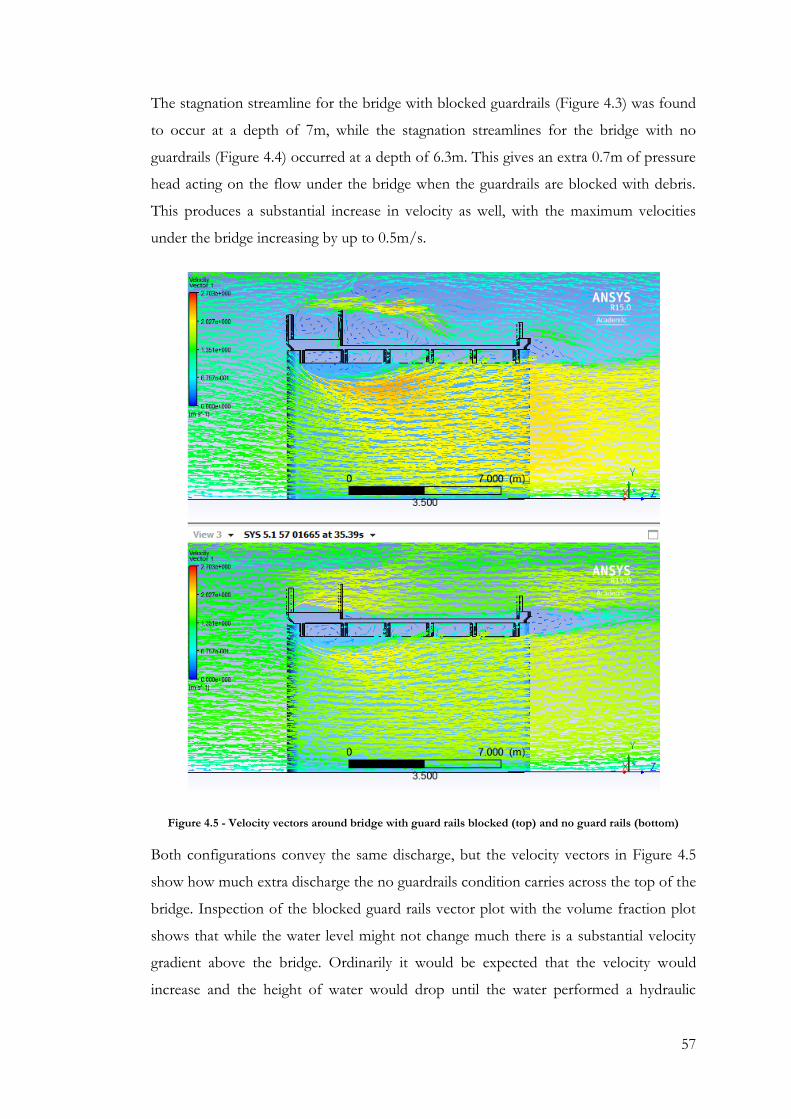
57

The stagnation streamline for the bridge with blocked guardrails (Figure 4.3) was found

to occur at a depth of 7m, while the stagnation streamlines for the bridge with no

guardrails (Figure 4.4) occurred at a depth of 6.3m. This gives an extra 0.7m of pressure

head acting on the flow under the bridge when the guardrails are blocked with debris.

This produces a substantial increase in velocity as well, with the maximum velocities

under the bridge increasing by up to 0.5m/s.

Figure 4.5 - Velocity vectors around bridge with guard rails blocked (top) and no guard rails (bottom)

Both configurations convey the same discharge, but the velocity vectors in Figure 4.5

show how much extra discharge the no guardrails condition carries across the top of the

bridge. Inspection of the blocked guard rails vector plot with the volume fraction plot

shows that while the water level might not change much there is a substantial velocity

gradient above the bridge. Ordinarily it would be expected that the velocity would

increase and the height of water would drop until the water performed a hydraulic

58

jump. It is possible that the initialisation or boundary conditions are affecting the

behaviour of the water at this point over the bridge. It could be that the water that is

being initialised at this point is becoming stagnant due to the flow around it. Without

running the simulation from a domain with entirely air and allowing the water to flow

into the domain on its own, it is not be possible to determine whether the options

selected are limiting the accuracy of the model. The blocked guard rail simulation has

velocities of 2m/s up to 25m past the end of the bridge.

Figure 4.6 - Velocity vectors near bridge pier with blocked guardrails (left) and no guardrails (right)

Figure 4.6 is taken from a plane 0.2m away from the edge of the pier. The streamline

and vector plots also show that the regardless of the guardrail condition there is a large

amount of turbulence below the bridge decking around the pier. This is expected as this

is the point of greatest flow constriction for the model.

59

4.4 Bed Shear Plots

Figure 4.7 – Topographic comparison of bed shear with blocked guardrails (left) and no guardrails (right) Upstream is at the top of image

Comparison of the bed shear plots in Figure 4.7 shows that when the guardrails are

blocked with debris the bed experiences a substantial amount more shear. Interpretation

from the plots shows the average maximum shear under the bridge around 40 Pa with

blocked guard rails and around 30 Pa with no guard rails. This corresponds to a 25%

difference in shear, which is quite significant considering the guard rails are only

blocking approximately 14% of the flow area.

It is important to reiterate that the shear stress values obtained here are only indicative,

and are based off surface roughness values that are almost certainly an overestimate.

The data gathered from this model can be adjusted when more accurate stream bed data

becomes available.

For a shear stress of 40 Pa, the maximum particle size that would be transported is

4.4cm, and for a shear stress of 30 Pa the maximum size is 3.3cm. With more accurate

data for the roughness of the streambed the correct maximum size particle could be

found. This does indicate however that the degree of scour around the bridge could be

substantially reduced if the debris on the guard rails of the bridge is managed.

60

Additionally there is another increase in the shear stress after the bridge with blocked

guardrails that does not appear on the simulation with no guard rails. Investigation of

stream lines and vector plots show a large increase in the downward velocity of the

water after the water exits from underneath the bridge. Presumably this is because the

water flowing over the blocked guardrails decreases in velocity substantially while water

flowing under the bridge increases velocity due to the effect of the pressurised flow.

The effect of combining these two flows is essentially a compressive action on the water

below the bridge that increases the shear stress on the bed of the channel. The

difference in velocities for the simulation with no guard rails is far less, which leads to a

far smaller and less violent combination. Figure 4.8 shows the velocity vectors around

the bridge; the length of the vector is the absolute magnitude of the velocity and the

vectors are coloured by the magnitude of their downward vertical velocity component.

Figure 4.8 - Velocity vectors with blocked guardrails (top) and no guardrails (bottom). Colour scale shows negative vertical velocity. Right is upstream.

61

It is important to consider that as the scour transports sediment the shear stress profile

would change and the flow regimes around the bridge would change as well. The

location of the maximum shear areas on the model correspond with the location of the

proposed scour hole in the base of the river shown in Figure 3.3, which gives an

indication that the turbulence shown here could be representative of reality.

An unexpected result from the vector and shear plots is that the flow is very asymmetric

about the bridge pier. The cause of this is not known, but the same style of turbulence

was experienced in various runs of the model, with different turbulence solvers and

different meshes. It is possible that for the trailing half of the bridge the turbulence

from the pier and the turbulence from the bridge decking combine to maximise their

effects, while on the leading half the turbulent conditions work to cancel each other out.

4.5 Limitations

While 3D CFD models are powerful tools, there are some limitations that impact the

accuracy of this study.

A critical step in creating an accurate CFD model is validating the model by comparing

it to experimental data. Since there was no experimental data to be compared to, the

accuracy of this model is unknown.

Time constraints and the size of the physical object meant that a relatively coarse grid

was chosen. Ordinarily a full grid independence study would be conducted to ensure

that the result is independent of the mesh specified. A previous run of the model with a

more coarse mesh around the bridge showed twice as many cells with a limited

turbulent viscosity ratio. The finer mesh had a higher cell density in the problem area,

which gives an indication that the final mesh is more accurate. However, due to the

length of time required to run the model a comprehensive grid independence study was

not able to be completed. The coarse nature of the mesh gives an imprecise indication

of the location of the water surface. Using a finer mesh would have produced more

accurate results.

Initially both the tallest and shortest sections of the bridge were intended to be

modelled, as this would give an indication of the effect of the rails at the extremes of

their height relative to the depth of the channel. Only the deepest section was modelled,

which is within the channel banks. Flow within channel banks typically encounters less

62

friction than flow over the floodplains due to the makeup of the stream bed compared

to grass that is generally on floodplains. When modelling individual sections it’s

important to consider the ability of water to move sideways in relation to flow

obstructions. In reality these sections are not operating in isolation from one another

and the entire length of the bridge will share the increase in backwater caused by the

flow obstruction. Modelling the whole bridge is unfeasible in the scope of an

undergraduate dissertation.

The Transition SST turbulence model was chosen as it was more robust than the k-ε

turbulence model, however, Menter (2009) found that the SST model had a tendency to

overestimate the size of turbulent eddies in some applications. A previous study by Zhu

Zhi-wen (2012) found that the k-ε turbulence model accurately modelled the process by

which scour happens but not the locations of the scour. Without validating data it is not

possible to comment on the accuracy of the chosen turbulence model.

The initialisation method chosen set the whole domain to the same volume fraction as

the inlet boundary, which means the model was initialised with the all fluid zones below

the water surface level being occupied by water. Initialising the model in this way may

not represent the final conditions in reality, since the depth of the water increases

gradually as the flood progresses, which could trap air under the bridge deck. Hydraulics

of Bridge Structures (Bradley 1978) states that air trapped in the bridge girders can

cause enough floatation to lift the bridge deck off the piers and shift it downstream. By

initialising water between the bridge girders the opportunity for air to be trapped under

the bridge decking never occurred. The presence of air between the girders could

change the flow considerably.

The boundary conditions chosen may be limiting the extent of the afflux. While there

was no literature found that explained the boundary conditions effect on the rest of the

model, the ANSYS manual seemed to indicate that specifying the velocity and depth for

the inlet was essentially the same as specifying the discharge, and posts on forums and

open channel flow CFD simulation videos corroborated this. However, without

running the simulation with the inlet at varying distances away from the bridge it’s

difficult to comment on the boundary conditions effects on the outcome of the model.

Additionally, the model was always run with a free surface level specified at the outlet.

Running the simulation without this may have changed the results. A combination of

63

the inlet conditions and the initialisation could be affecting the height of the flow

directly above the bridge.

4.6 Future Work

A grid independence study would need to be conducted in order to verify that the

results of the model are not being affected by the resolution of the mesh. For this study

the resolution of the model would be decreased until the results of the model stop

changing. Investigations into the effect of the inflation layers and body sizing functions

would also need to be undertaken.

In order to validate the model a scale physical model could be produced. A scale model

would be able to show the styles of turbulence experienced and the backwater generated

by the bridge. Once the CFD model has been validated by the physical model a

parametric study could be conducted including altering the porosity of the rails, as well

as the style of the rails to find a more hydraulically efficient rail configuration.

Validation of the model would include investigation into different turbulence models.

A different section of the bridge with a different obvert height should be modelled to

give a more complete picture of the effect of the rails. If the flow area obstructed by the

rails is increased relative to the depth of the water the effect of the rails would be

increased. The scenario explored in this project is the scenario where the rails would

have the least impact. A section of bridge with the piers on the symmetry planes and the

span of the bridge central could be modelled as well to confirm that the turbulence

being experienced is consistent.

The I-beam girders themselves do not seem to affect the degree of flow under the

bridge as much as the blocked guardrails. However, the bridge may convey more flow if

the girders are covered in some manner to produce a smoother underneath of the

bridge. An example may be a thin steel plate placed over the girders. Further study is

required to quantify the effect.

The model could be run in a more transient manner, with the domain initially air and

with boundary conditions that gradually increase the height of the water to investigate

the interaction between water and air around the girders. This could also give more

64

insight into how the backwater increases with time, as it is probable that the worst

backwater condition occurs when the water is in contact with the guard rails but not

flowing over them yet.

While this study was not primarily concerned with scour, from the literature review it’s

apparent that CFD is a powerful tool in modelling scour. The model could be modified

with a transportable channel bed as demonstrated in Submerged Flow Bridge Scour

Under Clear Water Conditions (Federal Highway Administartion 2012) and the effect of

scour around the piers on the O.O. Madsen bridge could be investigated. While the

O.O. Madsen Bridge has survived several large flood events this is no guarantee that

scour will not affect the bridge in the future.

65

Chapter 5

Conclusions and Recommendations

The O.O. Madsen Bridge experiences severe debris blockage in the guard rails when the

bridge is overtopped during large flood events. The local population believe the

blockage is leading to an increased depth of water upstream of the bridge during floods.

A 2D flood model of the Condamine River determined that the change in depth

immediately upstream of the bridge by removing the debris blocked guardrails was up

to 0.20m.

2D flood models provide councils and state governments with important tools for

planning and disaster mitigation. However, the assumptions and simplifications made in

order to produce a comprehensive model within reasonable time frames may not hold

true when interrogated on a small scale. In order to explore the accuracy of the

simplifications to the O.O. Madsen in the Condamine River Flood Study a 3D CFD

model was created.

A 3D CFD model of a section of the O.O. Madsen Bridge was created in ANSYS

Fluent. The CFD model allowed the bridge to be modelled in far greater detail than the

2D flood model. Even with this greater detail the minimum limit of confidence of the

model was 0.130m. The model allowed not only the afflux caused by the guardrails to

be investigated, but the turbulence and shear stress on the river bed caused by the

bridge and guard rails were also determined.

From the simulations performed the afflux caused by the first two guard rails being

100% blocked with debris was 8cm, with a further 9cm drop in the height of water after

the bridge from the energy loss of the water travelling over the bridge. Both values are

less than the minimum limits of confidence due the size of the grid used. The

simulation without guard rails showed no discernible change in surface water elevation.

With the current grid size it’s not possible to comment on the accuracy of the heights

66

produced, but the fact that there is a difference between the two simulations means that

the debris blocked guardrails do have an effect on flood depths.

The CFD simulation was not able to produce the same results as the 2D model by

Jacobs. This could be related to the limitations of the CFD study. The primary

limitation of this study was the scale of the object being modelled. Due to the size of

the bridge only a single section was simulated. The section modelled was the tallest,

which is the section with the least relative flow area blocked by guard rails. Individual

sections of the bridge do not operate hydraulically in isolation however, and the waters

ability to move sideways would ensure that the height of water across the bridge is

relatively constant along the length. Even though this section of the bridge does not

produce an afflux as large as the 2D Condamine River Flood Study, the bridge as a

whole would likely generate a larger afflux.

The results presented are unable to be verified as accurate. The inability to conduct a

grid independence study means that it is unknown whether the mesh used is affecting

the results. Without validating data it is not possible to confirm the flow patterns and

turbulence experienced, which could impact the accuracy of the results produced.

Within these limitations the model still shows that when blocked with debris the

guardrails have a substantial impact on the flow conditions experienced around the

O.O. Madsen Bridge, especially underneath the bridge. The guardrails increased the

height of the stagnation streamline by 0.7m, adding excess pressure head to the water

travelling under the bridge, increasing its velocity. This extra velocity increased the

average shear stress experienced on the river bed by 25%. The reduced velocity of the

flow travelling over the bridge caused substantial turbulence when it joined the high

speed flow from underneath the bridge. This turbulence added another area of high

shear stress that was not experienced on the model without guard rails. It was not

initially a consideration of this study that the guardrails would affect flow underneath

the bridge as much as they did.

Even though accurate backwater data was not able to be obtained from the model, the

data gathered suggests that more hydraulically efficient guard rails should be employed

at the O.O. Madsen Bridge. The current guards likely contribute to scour experienced

around the bridge. A study of scour around the O.O. Madsen was not found during the

literature review, so it is recommended that one is undertaken. While the cost to

67

community from backwater was estimated at $74,200 (Jacobs 2012) per year, the cost of

damage to the bridge from scour and the interruption of a vital transport road could be

far greater.

Due to the size of the object and the computation times required to achieve accurate

results, producing a CFD model of a complete bridge for every 2D flood model is not

practical. Instead fully validated CFD models could prove very useful in comparing

various bridge and guard rail designs, or improving the hydrodynamics of bridges that

are likely to be overtopped. The ability to compare turbulence and shear or scour

accurately for various bridge designs gives CFD modelling a distinct advantage over

basic empirical equations or 2D flood models.

68

Chapter 6 References

ABS 2011, Warwick, 2011 Census QuickStats, Australian Bureau of Statistics, viewed 30 May, <http://www.censusdata.abs.gov.au/census_services/getproduct/census/2011/quickstat/UCL313007>.

Anderson, LD 1995, Computational Fluid Dynamics: The Basics with Applications, McGraw-Hill, Inc.

ANSYS 2011, Turbulence Modelling, 275 Technology Drive Canonsburg, PA 15317, U.S.A.

ANSYS 2012, Multiphase Modelling in Automotive Industries.

ANSYS 2014, ANSYS Workbench User Manual.

Australia, S 2004, Bridge Design - Scope and General Principals, AS 5100.1, Standards Online.

B.C. Phillips, SY, G.R. Thompson and N. de Silva 2005, '1D and 2D Modelling of Urban Drainage Systems using XP-SWMM and TUFLOW', in 10th Internation Conference on Urban Drainage: proceedings of the10th Internation Conference on Urban Drainage Copenhagen/Denmark.

Bradley, JN, Hydraulics of Bridge Waterways, 1978, BD Federal Highway Administartion.

DTMR, Hydraulic Guidelines for Bridge Design Projects, 2013, DoTaMR Queensland, Online Technical Document.

Engineers, UACo 2014, HEC-RAS River Analysis Manual CPR-69 CEIW, US Army Corps of Engineers, viewed 27 May, <http://www.hec.usace.army.mil/software/hec-ras/>.

Federal Highway Administartion, BD, Submerged Flow Bridge Scour Under Clear Water Conditions, 2012, USDo Transportation, Turner-Fairbank Highway Research Center.

Gillies, M 2013, ENV3104 - Hydraulics II Module 6 - Sediment Transport, University of Southern Queensland, Toowoomba.

69

IJmker, S, Huysmans, M, Blatter, BM, van der Beek, AJ, van Mechelen, W & Bongers, PM 2007, 'Should office workers spend fewer hours at their computer? A systematic review of the literature', Occupational and Environmental Medicine, vol. 64, no. 4, pp. 211-22.

Jacobs 2012, Condamine River and Tributaries Flood Study Final Report.

Kerenyi, K, Sofu, T & Guo, J, Hydrodynamic Forces on Inundated Bridge Decks, 2009, Report No. FHWA-HRT-09-028.

Lanfrit, M 2005, Best Practice Guidelines for Handling Automotive External Aerodynamics with FLUENT.

Menter, FR 2009, 'Review of the Shear-Stress Transport Turbulence Model Experience from an Industrial Perspective', Int. J. of Comp. Fluid Dynamics, vol. 23, no. 4, pp. 305-16.

Parola, AC 2000, Debris Forces on Highway Bridges, National Cooperative Highway Research Program.

Pender, SNaG, Desktop review of 2D hydraulic modelling packages, 2009, DfEFaR Affairs, Environment Agency.

Syme, B 2011, 'Pro's and Cons of 1D and 2D Modeling', in FMA Converence: proceedings of theFMA Converence San Diego.

TMR, Bridge Scour Manual, 2013, DoTaMR Queensland.

Trucano, WLOaTG 2000, Validation Methodology in Computational Fluid Dynamics, Sandia National Laboratories, Albuquerque, New Mexico 87185-0828.

Wardhana, K & Hadipriono, FC 2003, 'Analysis of recent bridge failures in the United States', Journal of Performance of Constructed Facilities, vol. 17, no. 3, pp. 144-50.

WBM, B 2007, TUFLOW User Manual

Weeks, W, Witheridge, G, Rigby, E, and, AB & O‘Loughlin, G 2013, Project 11: Blockage of Hydraulic Structures.

Zhu Zhi-wen, LZ-q 2012, CFD prediction of local scour hole around bridge piers, Central South University Press and Springer-Verlag Berlin Heidelberg.

70

Appendix A

Project Specification

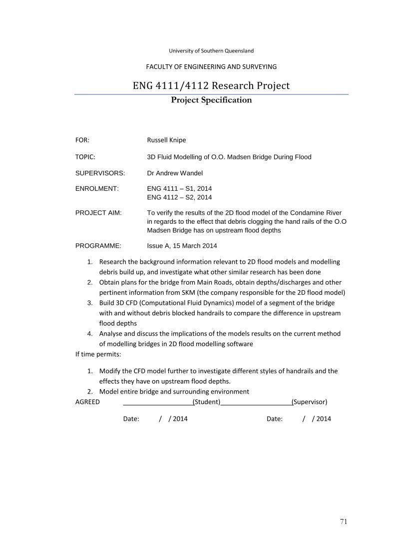
71

University of Southern Queensland

FACULTY OF ENGINEERING AND SURVEYING

ENG 4111/4112 Research Project

Project Specification

FOR: Russell Knipe

TOPIC: 3D Fluid Modelling of O.O. Madsen Bridge During Flood

SUPERVISORS: Dr Andrew Wandel

ENROLMENT: ENG 4111 – S1, 2014

ENG 4112 – S2, 2014

PROJECT AIM: To verify the results of the 2D flood model of the Condamine River

in regards to the effect that debris clogging the hand rails of the O.O

Madsen Bridge has on upstream flood depths

PROGRAMME: Issue A, 15 March 2014

1. Research the background information relevant to 2D flood models and modelling

debris build up, and investigate what other similar research has been done

2. Obtain plans for the bridge from Main Roads, obtain depths/discharges and other

pertinent information from SKM (the company responsible for the 2D flood model)

3. Build 3D CFD (Computational Fluid Dynamics) model of a segment of the bridge

with and without debris blocked handrails to compare the difference in upstream

flood depths

4. Analyse and discuss the implications of the models results on the current method

of modelling bridges in 2D flood modelling software

If time permits:

1. Modify the CFD model further to investigate different styles of handrails and the

effects they have on upstream flood depths.

2. Model entire bridge and surrounding environment

AGREED (Student) (Supervisor)

Date: / / 2014 Date: / / 2014

72

Appendix B

Project Timeline

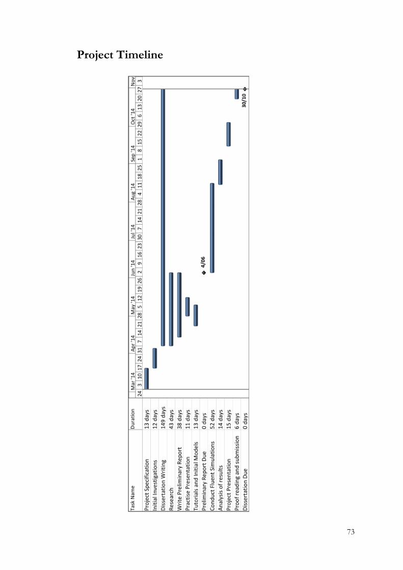
73

Project Timeline

74

Appendix C

Risk Assessment

75

Risk Assessment

There are 6 steps in performing a risk assessment:

1. Identify the Hazard

2. Identify the Risk

3. Assess the Risk

4. Control the Risk

5. Document the Process

6. Monitor and Review

Identifying the hazard involved identifying potentially sources of risk. Once the source

of the risk has been identified the risk itself is identified and quantified so it can be

assessed. Assessing the risk requires use of a risk matrix. First the likelihood of the

hazard is identified, then the consequences. These two attributes are entered into the

matrix and the risk is identified. Controlling the risk requires that measures be put in

place to either reduce the likelihood, mitigate the consequences or both. The risk is then

reassessed to see what the new risk is. The risk matrix is shown in Figure C.6.1.

Steps 5 and 6 are not necessarily relevant in the context of this project, and as such only

steps 1 through 4 will be undertaken.

Figure C.6.1 - Risk Assessment Matrix

76

Hazard Extended time spent using computers

The project involves CFD calculations which can take a large amount of time. Studies

have shown that spending large amounts of time in front of computers can lead to eye

damage and muscular skeletal issues.

Likelihood Likely

Consequences Major

Risk High

Control Measures Reduce brightness of monitor

Limit length of computer sessions

Stretch and exercise frequently

Reduced Risk Medium – Hazard still needs to be monitored

Hazard Consequences of Project

The project deals with guard rails and the effect they have on flood depths upstream of

the bridge. Flooding affects people’s property and lives, and the findings of this project

could potentially influence future decisions made regarding the configuration of the

guard rails, which likewise affects the people upstream of the O.O. Madsen.

Likelihood Possible

Consequences Severe

Risk High

Control Measures Thoroughly complete project to highest standard possible

Identify and state all sources of potential inaccuracies

Validate model to experimental data

Reduced Risk Medium – Hazard still needs to be monitored

77

Appendix D

Model Version Log

78

Version Date File Name Changes Made Comments

Alpha 27/03/2014 Practise Single Phase Ahmed Body - Fluent Familiarisation

1.01 10/04/2014 Flow Empty domain, transient, gravity set, multiphase VoF method, k-epsilon turbulent solver

Attempted two phase flow - model not converging

1.02 15/04/2014 Fluidstuff Open Channel Flow, Pressure inlet boundary, pressure outlet boundary, top boundary pressure outlet

Model not converging, air leaving out top boundary

1.03 15/05/2014 Working Top Boundary set to wall, Initialisation methods set following ANSYS user guide

Model converging, but it’s not apparent whether the solutions are working as expected in the empty domain

1.04 19/05/2014 Working Cylindrical "pier" placed in path of flow

Model not converging

1.05 21/05/2014 Working Growth rate set to 1.1, Added body for water surface, added face sizing and body sizing functions

Model was not converging before face sizing function was introduced to pier, and growth rate reduced to 1.1, surface indistinct until body sizing function introduced

1.06 30/05/2014 Working Top boundary layer changed to pressure outlet, pressure inlet, mass flow inlet

All boundary's except wall create a suction effect where air leaves out the top boundary

1.1 30/06/2014 Working Geometry Began modelling bridge geometry - still learning how to use the geometry program

1.11 1/07/2014 Working Geometry, meshing Bridge geometry complete, have not moved geometry into fluent file

1.12 2/07/2014 Working Imported bridge geometry into fluent from pier model, reset boundary condition surface levels and velocities, adjusted growth rate to 1.1, coarse mesh

Model not converging even after mesh adjusted. Need to try first aspect ratio inflation

1.13 15/07/2014 Bridge First aspect ratio set Model now converging, 4.8 million elements, roughly 20 mins of calculations for convergence, very low drop of water over bridge

79

1.14 22/07/2014 Bridge Output interpretation Spent several hours experimenting with Fluent and CFD-Post output's to create usable results, still insignificant drop over bridge

1.14 25/07/2014 No Rails Geometry - Removed Guardrails, re-meshed

Deleted guardrails and re ran calculations, model takes roughly the same amount of time to converge and there is very little perceivable difference in water heights across bridge from the model with rails

1.15 7/08/2014 Bridge Geometry and meshing - added body sizing function

Body sizing function added for water surface, similar to the cylindrical pier before, gives a much more usable surface profile

1.16 19/08/2014 Bridge Outlet boundary = 2.5m

The outlet boundary was changed to be 0.5m lower than the inlet boundary, to reflect the results of the Jacobs model. No significant change in surface profile was observed

1.16 25/08/2014 No Rails No rails with body sizing function

Similar result to above

1.17 29/08/2014 Bridge Rail faces - Named selections - set to porous jump

Gave the faces of the rail their own named selection, set them to a porous jump in attempt to create permeable rails. No effect

1.18 3/09/2014 Bridge Porous jump options changed

Tried various different options for porous jump based on calculations presented in the ANSYS documentation but to no effect

2.0 6/09/2014 060914 Bridge geometry changed

Initial bridge geometry’s failed to model the I beam girders beneath the bridge deck. The girders increase the profile of the bridge deck that is perpendicular to flow by over 200%

2.1 7/09/2014 070914 Meshing - medium smoothing, removed first aspect ratio inflation

I beam girders not meshing, the profiles are too fine for the meshing program to accurately reproduce with such a coarse mesh, and if the mesh is made finer it will make computation too lengthy

2.2 8/09/2014 080914 Geometry - modified Changed the I beam girders into rectangular boxes of the same width and height. Meshing now solves first aspect ratio inflation and will mesh with course sizing.

80

2.3 9/09/2014 090914 Finalised geometry, into fluent

Ran the model with the final bridge geometry with rails. Head loss over the bridge far more apparent than in previous versions. Suggests that a large amount of energy loss through the model is caused by the girders as well. Convergence was achieved in similar times

1.19 10/09/2014 Bridge Geometry - rails separated from bridge, changed to fluids, set with porosity of 0.8

Separated the rails from the bridge body, and modelled the rails as fluids. Previously water could not travel through because the rails were essentially outside the domain. Water now flows through the rails however the porosity does not seem to be affecting the ability of the water to flow through the section

2.4 10/09/2014 100914 New geometry with porous rails

Separated the new geometry into porous rails, same result as before with no noticeable effect due to the rails.

2.5 12/09/2014 120914 Porosity set from 0.01 to 0.99

Various porosity's were set for the rails; however none had any perceivable difference in the model.

2.6 14/09/2014 140914 Porosity removed, faces of rails set as porous jumps

The faces of the rails were set up as porous jumps. Initially there was no effect but after adjusting the parameters to increase the effect of the porous jump there was some effect. However the values entered are unrealistically high

1.07 16/09/2014 Porous Test

Bridge pier geometry - changed to wall

Experimenting with porosity on the full size domain was taking too much time, so the initial geometry was modified to test the effect of porosity. Similar problems with porosity occurred as with the full scale model, however it was discovered that the model requires more time to run.

81

1.08 16/09/2014 Porous Test

Test wall made solid Test wall was changed from a fluid to a solid. For all other runs the model was only run until the model converged, but in this test the model was run for a large amount of time after converging to see the effects. From this run it became obvious that the problem with the model was that the flow was not being allowed to develop properly. Future runs of all models will be run for a greater length of time

2.7 19/09/2014 190914 Rails set to solid, Run for 230 iterations

Model run for 1.9 seconds model time. Results more in line with what’s expected. Need to allow flow to develop further

2.8 19/09/2014 190914 - No rails

Rails set to fluid Model was run for .8 seconds model time, flow still developing

2.7 20/09/2014 200914 Run for 4.8 seconds At 4.8 seconds flow still changing. Velocity of wind is 8m/s in reverse direction

2.8 20/09/2014 200914 - No rails

Run for 3.5 seconds At 3.5 seconds flow still changing. Velocity of wind is 7.5m/s in reverse direction

2.7 21/09/2014 210914 Run for 7.5 seconds Wind travelling at 42m/s, creating substantial changes to surface of water. Model aborted.

2.8 21/09/2014 210914 - No rails

Run for 6.8 seconds Wind travelling at 42m/s, creating substantial changes to surface of water. Model aborted.

2.9 22/09/2014 220914 Outlet boundary = 3m, run for 4.4 seconds

The outlet boundary for the model was set back to the same height as the inlet, which in previous models has led to the air travelling at the same speed as the water. Fluid still developing but air travelling at sensible velocities. Wanted to run no rails model but not enough licenses available.

2.9 23/09/2014 230914 Run for 7.5 seconds Model began to take more iterations to solve each time step at 7.5 seconds. Still no extra licenses available

2.9 30/09/2014 300914 Run for 7.68 seconds Model began to diverge at 7.68 seconds. Possible that one of the eddy currents moved into a section of coarse mesh with the k-epsilon solver could not deal with. Model aborted

82

2.10 2/10/2014 021014 Turbulent solver set to transition SST

Model run for 3.6 seconds. So far model looks more stable and surface is more responsive to the bridge obstruction

03/10/14 to 10/10/14

No licenses available, no progress

2.10 11/10/2014 111014 Run for 11.78 seconds Model still stable and converging, however turbulent viscosity limited to viscosity ratio of 1.00000e+05 in 62 cells

3.1 11/10/2014 High-Res Mesh

Medium sizing, 1.07 growth rate

Tried many different ways of getting a mesh with medium smoothing and a 1.07 growth rate into the already established fluent model, but had a lot of difficulty. Eventually worked, but took model nearly 2 hours to converge. Time constraints make finer mesh prohibitive

2.10 12/10/2014 121014 Run for 21 seconds Model still converging, however viscosity ratio is limited in 700 cells.

2.11 12/10/2014 121014 - No rails

Run for 7.5 seconds Model converging nicely, no errors to report

2.10 13/10/2014 131014 Run for 29 seconds Model converging in a single iteration, inspection of plots reveals it appears to have achieved steady state. Viscosity ratio limited in 27,000 cells, however model has 6.5 million elements. Discussion with supervisor explained that viscosity ratio limits the amount of transport a model does and is not necessarily damaging to results. Model with rails is considered complete.

2.11 13/10/2014 131014 - No rails

Run for 15.2 seconds Model converging nicely, turbulent viscosity went up to 700 at one point but has decreased to 400

2.11 14/10/2014 141014 - No rails

Run for 22 seconds Model converging nicely, turbulent viscosity stable at around 360. Model appears to have achieved steady state earlier than the blocked rails model

2.11 15/10/2014 151014 - No rails

Run for 25 seconds Plots compared, model has achieved steady state. Model without rails is considered complete

83

3.20 18/10/2014 Final No Rails Geometry - Moved inlet boundary further away Meshing - Added body sizing function around bridge, 0.25m cells. Face sizing function on bridge faces, 0.05m. Fluent - Checked Zonal Discretization, lowered convergence to 1e-4

Zonal discretization specifies the discretization to compressive, which produces a much finer boundary layer. The resolution of the mesh around the bridge was increased in order to reduce the turbulent viscosity, and the inlet boundary was moved further away from the bridge to try and eliminate any interference with the height of the water. Time constraints make this the final version. Only first 2 rails blocked, 3rd rail set to fluid.

3.21 18/10/2014 Final - No rails

No Rails Geometry - Moved inlet boundary further away Meshing - Added body sizing function around bridge, 0.25m cells. Face sizing function on bridge faces, 0.05m. Fluent - Checked Zonal Discretization, lowered convergence to 1e-4

Zonal discretization specifies the discretization to compressive, which produces a much finer boundary layer. The resolution of the mesh around the bridge was increased in order to reduce the turbulent viscosity, and the inlet boundary was moved further away from the bridge to try and eliminate any interference with the height of the water. Time constraints make this the final version. All rails set to fluid

3.20 19/10/2014 Final 191014

Modelled to 2.2 seconds

Increased mesh resolution and convergence criteria has slowed model considerably. Solution stable, surface of water is being modelled with high fidelity

3.21 19/10/2014 Final - No rails 191014

Modelled to 2.1 seconds

Increased mesh resolution and convergence criteria has slowed model considerably. Solution stable, surface of water is being modelled with high fidelity

3.20 20/10/2014 Final 201014

Modelled to 3.0 seconds

Solution stable and continuing as expected

3.21 20/10/2014 Final - No rails 201014

Modelled to 3.1 seconds

Less turbulence is allowing the no rails model to solve faster

3.20 21/10/2014 Final 211014

Modelled to 6.7 seconds, timestep increased to 0.02s

Model is converging nicely, courant number shown at maximum of 2, so time-step increased

3.21 21/10/2014 Final - No rails 211014

Modelled to 7 seconds, timestep increased to 0.02s

Model is converging nicely, courant number shown at maximum of 2, so time-step increased

84

Appendix E

MATLAB Code

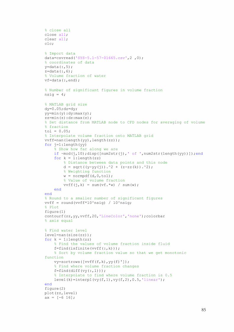
85

% close all close all; clear all; clc;

% Import data data=csvread('SYS-5.1-57-01665.csv',2 ,0); % coordinates of data y=data(:,5); z=data(:,6); % Volume fraction of water vf=data(:,end);

% Number of significant figures in volume fraction nsig = 4;

% MATLAB grid size dy=0.05;dz=dy; yy=min(y):dy:max(y); zz=min(z):dz:max(z); % Set distance from MATLAB node to CFD nodes for averaging of volume % fraction tol = 0.05; % Interpolate volume fraction onto MATLAB grid vvff=nan(length(yy),length(zz)); for j=1:length(yy) % Show how far along we are if ~mod(j,10);disp([num2str(j),' of ',num2str(length(yy))]);end for k = 1:length(zz) % Distance between data points and this node d = sqrt((y-yy(j)).^2 + (z-zz(k)).^2); % Weighting function w = normpdf(d,0,tol); % Value of volume fraction vvff(j,k) = sum(vf.*w) / sum(w); end end % Round to a smaller number of significant figures vvff = round(vvff*10^nsig) / 10^nsig; % Plot figure(1) contourf(zz,yy,vvff,20,'LineColor','none');colorbar % axis equal

% Find water level level=nan(size(zz)); for k = 1:length(zz) % Find the values of volume fraction inside fluid f=find(isfinite(vvff(:,k))); % Sort by volume fraction value so that we get monotonic

function vy=sortrows([vvff(f,k),yy(f)']); % Find where volume fraction changes f=find(diff(vy(:,1))); % Interpolate to find where volume fraction is 0.5 level(k)=interp1(vy(f,1),vy(f,2),0.5,'linear'); end figure(2) plot(zz,level) ax = [-6 16];

86

ylim(ax); line(11/2*[-1 -1; 1 1]',[ax;ax]') figure(1) hold on plot(zz,level,'r') hold off ylim([-6 16]) line (zz, 3)

% find average afflux upstream of the bridge upstrm = level(-40<zz & zz<-7); afflux = mean(upstrm);

% find average headloss of water after bridge dnstrm = level(7<zz & zz<40); hloss = mean(dnstrm);

87

Appendix F

Steady State Analysis

88

Figure 6.2 - Steady state volume fraction comparison, blocked guard rails

Figure 6.3 - Steady state volume fraction comparison, no guardrails

89

Appendix G

Comparison of CFD-Post, Fluent and

MATLAB Plots

90

Blocked Guard Rails

Figure 6.4 - CFD-Post node volume fraction plot – Blocked guard rails

Figure 6.5 - FLUENT cell centred volume fraction plot – Blocked guard rails

91

Figure 6.6 - MATLAB volume fraction plot from CFD-Post Export – Blocked guard rails

Figure 6.7 - MATLAB volume fraction plot from Fluent Export – Blocked guard rails

92

Figure 6.8 - Surface plot, blocked guard rails. Green and blue vertical lines represent location of bridge

Figure 6.9 - Volume fraction and surface plot, blocked guard rails – red line represents calculated water surface

93

No Guard Rails

Figure 6.10 - CFD-Post node volume fraction plot – No guard rails

Figure 6.11 - Fluent cell centre volume fraction plot - No guard rails

94

Figure 6.12 - MATLAB volume fraction plot from CFD-Post Export – No guard rails

Figure 6.13 - MATLAB volume fraction plot from Fluent Export – No guard rails

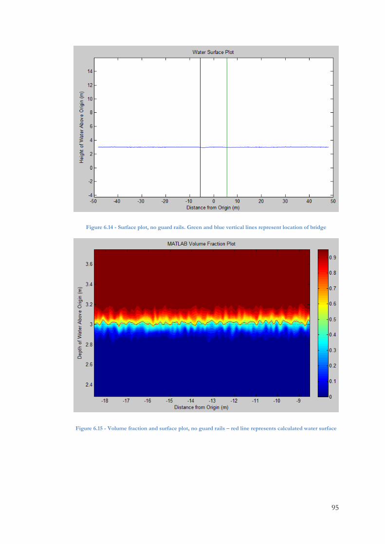
95

Figure 6.14 - Surface plot, no guard rails. Green and blue vertical lines represent location of bridge

Figure 6.15 - Volume fraction and surface plot, no guard rails – red line represents calculated water surface

96

Appendix H

Vector Plots

97

Figure 6.16 - Vector plot with guard rails blocked (Top) and no guard rails (Bottom)