3.5: Euler’s Method (cont’d) and 3.7: Population ModelingEuler’s Method Algorithm To calculate...
45
3.5: Euler’s Method (cont’d) and 3.7: Population Modeling Mathematics 3 Lecture 19 Dartmouth College February 15, 2010 – Typeset by Foil T E X –
Transcript of 3.5: Euler’s Method (cont’d) and 3.7: Population ModelingEuler’s Method Algorithm To calculate...

3.5: Euler’s Method (cont’d)and
3.7: Population Modeling
Mathematics 3Lecture 19
Dartmouth College
February 15, 2010
– Typeset by FoilTEX –
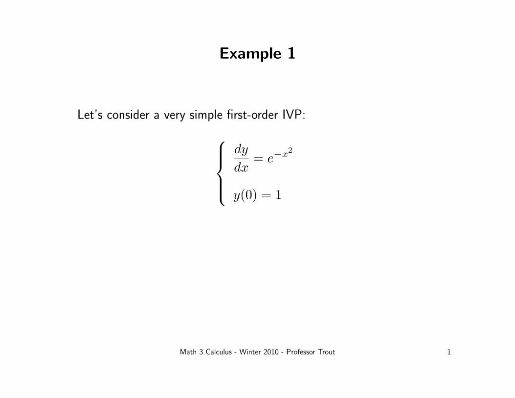
Example 1
Let’s consider a very simple first-order IVP:dy
dx= e−x2
y(0) = 1
Math 3 Calculus - Winter 2010 - Professor Trout 1

Example 1
Let’s consider a very simple first-order IVP:dy
dx= e−x2
y(0) = 1
This is clearly separable, so we try to solve as follows:
dy = e−x2dx =⇒ y =
∫e−x2
dx = ???
Math 3 Calculus - Winter 2010 - Professor Trout 1

Example 1
Let’s consider a very simple first-order IVP:dy
dx= e−x2
y(0) = 1
This is clearly separable, so we try to solve as follows:
dy = e−x2dx =⇒ y =
∫e−x2
dx = ???
Problem: There is NO known elementary formula for this integral!!!
Math 3 Calculus - Winter 2010 - Professor Trout 1

Recall: Euler’s Method Algorithm
To calculate a numerical approximate value to the solution value y(b) of
IVP
8>><>>:dy
dx= F (x, y)
y(x0) = y0
on the interval [x0, b] (where x0 < b) using N ≥ 1 steps:
1.) Use the increment h = ∆x = (b− x0)/N .
2.) Start with the initial (value) point P0 = (x0, y0). Set n = 0.
3.) Given the “old point”(xn, yn), the “next point”(xn+1, yn+1) of the approx-
imate solution is: xn+1 = xn+h
yn+1 = yn+hF (xn, yn)
4.) If n + 1 = N , xN = b, STOP. Use yN ≈ y(b). Otherwise increase n by
1 and GOTO Step 3.
Math 3 Calculus - Winter 2010 - Professor Trout 2

Recall: Euler’s Method Algorithm
To calculate a numerical approximate value to the solution value y(b) of
IVP
8>><>>:dy
dx= F (x, y)
y(x0) = y0
on the interval [x0, b] (where x0 < b) using N ≥ 1 steps:
1.) Use the increment h = ∆x = (b− x0)/N .
2.) Start with the initial (value) point P0 = (x0, y0). Set n = 0.
3.) Given the “old point”(xn, yn), the “next point”(xn+1, yn+1) of the approx-
imate solution is: xn+1 = xn+h
yn+1 = yn+hF (xn, yn)
4.) If n + 1 = N , xN = b, STOP. Use yN ≈ y(b). Otherwise increase n by
1 and GOTO Step 3.
NOTE: This algorithm also works if b < x0, we just change + in Step 3 to −.
Math 3 Calculus - Winter 2010 - Professor Trout 2

Example 1 (cont’d)
Let’s consider that unsolvable IVP:dy
dx= e−x2
y(0) = 1
Math 3 Calculus - Winter 2010 - Professor Trout 3

Example 1 (cont’d)
Let’s consider that unsolvable IVP:dy
dx= e−x2
y(0) = 1
a.) Use Euler’s method with N = 2 steps to approximate y(8).
Math 3 Calculus - Winter 2010 - Professor Trout 3

Example 1 (cont’d)
Let’s consider that unsolvable IVP:dy
dx= e−x2
y(0) = 1
a.) Use Euler’s method with N = 2 steps to approximate y(8).
Answer: y(8) ≈ y2 = 5 but actually y(8) = 1.88623... §
Math 3 Calculus - Winter 2010 - Professor Trout 3

Example 1 (cont’d)
Let’s consider that unsolvable IVP:dy
dx= e−x2
y(0) = 1
a.) Use Euler’s method with N = 2 steps to approximate y(8).
Answer: y(8) ≈ y2 = 5 but actually y(8) = 1.88623... §
b.) Use the Euler Method applet with the steps in the table below toapproximate y(8).
Math 3 Calculus - Winter 2010 - Professor Trout 3

Example 1 (cont’d)
b.) Use the Euler Method applet with the steps in the table below toapproximate y(8).
N h = ∆x yN
2 44 28 1
16 0.532 0.25
8,000 0.001
Math 3 Calculus - Winter 2010 - Professor Trout 4

Example 1 (cont’d)
b.) Use the Euler Method applet with the steps in the table below toapproximate y(8).
N h = ∆x yN
2 4 54 2 3.036638 1 2.38632
16 0.5 2.1362332 0.25 2.01123
8,000 0.001 1.88673
Recall that y(8) = 1.88623...
Math 3 Calculus - Winter 2010 - Professor Trout 5
Example 1 (cont’d)
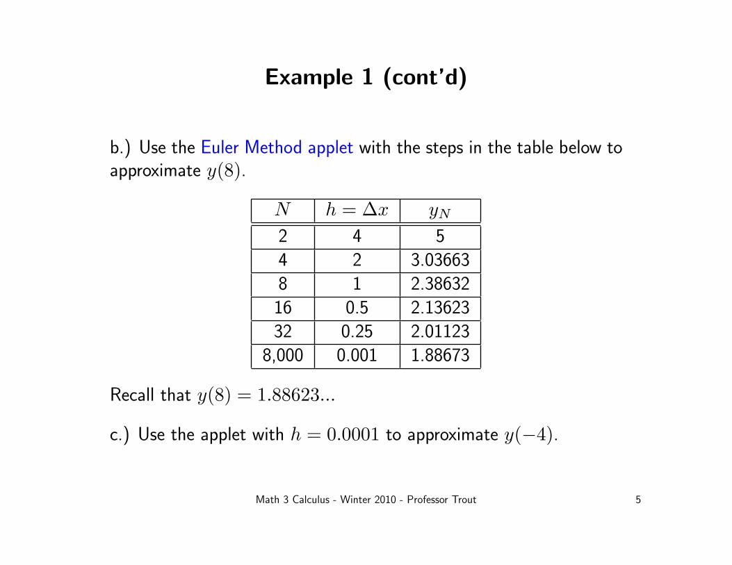
b.) Use the Euler Method applet with the steps in the table below toapproximate y(8).
N h = ∆x yN
2 4 54 2 3.036638 1 2.38632
16 0.5 2.1362332 0.25 2.01123
8,000 0.001 1.88673
Recall that y(8) = 1.88623...
c.) Use the applet with h = 0.0001 to approximate y(−4).
Math 3 Calculus - Winter 2010 - Professor Trout 5

Example 1 (cont’d)
b.) Use the Euler Method applet with the steps in the table below toapproximate y(8).
N h = ∆x yN
2 4 54 2 3.036638 1 2.38632
16 0.5 2.1362332 0.25 2.01123
8,000 0.001 1.88673
Recall that y(8) = 1.88623...
c.) Use the applet with h = 0.0001 to approximate y(−4).
Ans: y(−4) ≈ 0.11372 which is good since y(−4) = 0.113773...
Math 3 Calculus - Winter 2010 - Professor Trout 5

Example 2
Consider the (nonseparable) IVP:dy
dx= x sin(xy)
y(−4) = 5
Use the Euler Method applet to find the increment size h = ∆x thatwill give an approximation to the actual solution value
y(9) = 2.446829...
accurate to 4 decimal places.
Math 3 Calculus - Winter 2010 - Professor Trout 6

Example 2
Consider the (nonseparable) IVP:dy
dx= x sin(xy)
y(−4) = 5
Use the Euler Method applet to find the increment size h = ∆x thatwill give an approximation to the actual solution value
y(9) = 2.446829...
accurate to 4 decimal places.
Answer: When h = 0.01, y(9) ≈ 2.44683 accurate to 4 decimals.
Math 3 Calculus - Winter 2010 - Professor Trout 6

How to Build (Better) Mathematical Models
1. Translate real-world problems into mathematical models.
Math 3 Calculus - Winter 2010 - Professor Trout 7

How to Build (Better) Mathematical Models
1. Translate real-world problems into mathematical models.
2. Subject the models to mathematical analysis and prediction.
Math 3 Calculus - Winter 2010 - Professor Trout 7
How to Build (Better) Mathematical Models
1. Translate real-world problems into mathematical models.
2. Subject the models to mathematical analysis and prediction.
3. Draw conclusions from the models.
Math 3 Calculus - Winter 2010 - Professor Trout 7

How to Build (Better) Mathematical Models
1. Translate real-world problems into mathematical models.
2. Subject the models to mathematical analysis and prediction.
3. Draw conclusions from the models.
4. Test the conclusions in the laboratory and compare the results withthe original real-world data.
5. Revise the model as necessary and repeat the above steps until themodel is a reliable predictor of real-world observations.
Math 3 Calculus - Winter 2010 - Professor Trout 7

3.7: Case Study: Population Modeling
Objective: Predict the size of the population of the United Stateswell into the 21st century.
Math 3 Calculus - Winter 2010 - Professor Trout 8

3.7: Case Study: Population Modeling
Objective: Predict the size of the population of the United Stateswell into the 21st century.
Math 3 Calculus - Winter 2010 - Professor Trout 8

Population Census Data of the United States
The U.S. Census Bureau is required by the U. S. Constitution to doa national census of the population every 10 years.
Math 3 Calculus - Winter 2010 - Professor Trout 9

Population Census Data of the United States
The U.S. Census Bureau is required by the U. S. Constitution to doa national census of the population every 10 years.
We will use only the populations recorded in the census of the years1790, 1990 and 2000:
Year Population (millions)
1790 3.91990 248.72000 281.4
Math 3 Calculus - Winter 2010 - Professor Trout 9

The Malthus Population Model
Math 3 Calculus - Winter 2010 - Professor Trout 10

The Malthus Population Model
• The Malthus model for growth of a population assumes an idealenvironment.
Math 3 Calculus - Winter 2010 - Professor Trout 10

The Malthus Population Model
• The Malthus model for growth of a population assumes an idealenvironment.
• Resources are unlimited, disease is constrained, and individuals arehappy.
Math 3 Calculus - Winter 2010 - Professor Trout 10

The Malthus Population Model
• The Malthus model for growth of a population assumes an idealenvironment.
• Resources are unlimited, disease is constrained, and individuals arehappy.
• The population increases at a rate proportional to the number ofindividuals present.
Math 3 Calculus - Winter 2010 - Professor Trout 10

Malthus Model: Exponential Growth
Q = Q(t) be the population of the USA (in millions) at time t.t = number of years since the 1790 census.
Math 3 Calculus - Winter 2010 - Professor Trout 11

Malthus Model: Exponential Growth
Q = Q(t) be the population of the USA (in millions) at time t.t = number of years since the 1790 census.
Starting with a population of 3.9 million in 1790, we have the IVP:dQ
dt= kQ
Q(0) = 3.9
Math 3 Calculus - Winter 2010 - Professor Trout 11

Malthus Model: Exponential Growth
Q = Q(t) be the population of the USA (in millions) at time t.t = number of years since the 1790 census.
Starting with a population of 3.9 million in 1790, we have the IVP:dQ
dt= kQ
Q(0) = 3.9
Example 3 Use the Malthus model to do the following:a.) Use the Population Modeling applet to guess the right value of kto give the 1990 census figure (at t = 200) and check your answeralgebraically.b.) Estimate the US populations in 2000 and 2010 and analyze theresults. Is the Malthus model a good predictor?
Math 3 Calculus - Winter 2010 - Professor Trout 11

The Verhulst Population Model
The Verhulst model assumes that the growth rate declines, from avalue k when conditions are very favorable, to the value 0 when thepopulation has increased to the maximum value M that the environ-ment can support.
Math 3 Calculus - Winter 2010 - Professor Trout 12

The Verhulst Population Model
The Verhulst model assumes that the growth rate declines, from avalue k when conditions are very favorable, to the value 0 when thepopulation has increased to the maximum value M that the environ-ment can support.
Takes into account the effects of a limiting environment.
It is a more realistic model.
Math 3 Calculus - Winter 2010 - Professor Trout 12

Verhulst Model: Limited Exponential Growth
The Verhulst model assumes that the growth rate declines, from avalue k when conditions are very favorable, to the value 0 when thepopulation has increased to the maximum value M that the environ-ment can support.
Math 3 Calculus - Winter 2010 - Professor Trout 13

Verhulst Model: Limited Exponential Growth
The Verhulst model assumes that the growth rate declines, from avalue k when conditions are very favorable, to the value 0 when thepopulation has increased to the maximum value M that the environ-ment can support.
It replaces the growth constant k by the algebraic expression
k(M −Q(t)
M
)
This leads to the differential equation
dQ
dt= k
(M −Q
M
)Q.
Math 3 Calculus - Winter 2010 - Professor Trout 13

The factor M−QM has a value between 0 and 1:
0 ≤ M −Q
M≤ 1
and is sometimes called the unrealized potential for pop. growth.
Math 3 Calculus - Winter 2010 - Professor Trout 14

The factor M−QM has a value between 0 and 1:
0 ≤ M −Q
M≤ 1
and is sometimes called the unrealized potential for pop. growth.
When Q is small (Q ≈ 0) we have that this factor
M −Q
M≈ 1 =⇒ k
(M −Q
M
)Q ≈ kQ
and the growth of the population is essentially exponential.
As Q approaches its asymptotic limiting value (Q ↗ M), however,the factor
M −Q
M↘ 0
is close to zero, and the population grows ever more slowly. [See GC]
Math 3 Calculus - Winter 2010 - Professor Trout 14

Objective
• The U.S. population cannot sustain exponential growth indefi-nitely.
• The Malthus model gives unrealistic projections of the populationover the next century.
• We would like to use the Verhulst model instead to make suchprojections.
• We also need to assume that Q(0) = 3.9 million, and M = 750million, the maximum value of the population (0 ≤ Q(t) ≤M).
Math 3 Calculus - Winter 2010 - Professor Trout 15

Verhulst U.S. Population Model
dQ
dt= k
(750−Q
750
)Q
Q(0) = 3.9
Math 3 Calculus - Winter 2010 - Professor Trout 16

Verhulst U.S. Population Model
dQ
dt= k
(750−Q
750
)Q
Q(0) = 3.9
Example 4 Use the Verhulst U.S. population model to do the fol-lowing:
a.) Predict with the Population Modeling applet using k = 0.0228the US population in the years 1990, 2000 and analyze the results. Isthis a better model than the Malthus model?
b.) Now estimate the US population in the years 2010 and 2020.
Math 3 Calculus - Winter 2010 - Professor Trout 16