31, 2012 . 6. PERFORMING ORGANIZATION CODE 7. AUTHOR(S) Balabhaskar Balasundaram . Satish T.S....

OTCREOS9.1-02-F

ECONOMIC ENHANCEMENT THROUGH INFRASTRUCTURE STEWARDSHIP

PROACTIVE APPROACH TO TRANSPORTATION RESOURCE ALLOCATION UNDER SEVERE

WINTER WEATHER EMERGENCIES

BALABHASKAR BALASUNDARAM, PH.D.

SATISH T. S. BUKKAPATNAM, PH.D. ZHENYU KONG, PH.D.

YANG HONG, PH.D.

Phone: 405.732.6580

Fax: 405.732.6586

www.oktc.org

Oklahoma Transportation Center

2601 Liberty Parkway, Suite 110

Midwest City, Oklahoma 73110

http://www.oktc.org

DISCLAIMER

The contents of this report reflect the views of the authors, who are responsible for the facts and

accuracy of the information presented herein. This document is disseminated under the sponsorship

of the Department of Transportation University Transportation Centers Program, in the interest of

information exchange. The U.S. Government assumes no liability for the contents or use thereof.

i

TECHNICAL REPORT DOCUMENTATION PAGE

1. REPORT NO. OTCREOS9.1-02-F

2. GOVERNMENT ACCESSION NO. 3. RECIPIENT’S CATALOG NO.

4. TITLE AND SUBTITLE Proactive Approach to Transportation Resource Allocation Under Severe Winter Weather Emergencies

5. REPORT DATE January 31, 2012 6. PERFORMING ORGANIZATION CODE

7. AUTHOR(S) Balabhaskar Balasundaram Satish T.S. Bukkapatnam Zhenyu Kong Yang Hong

8. PERFOMING ORGANIZATION REPORT

9. PERFORMING ORGANIZATION NAME AND ADDRESS Oklahoma State University, School of Industrial Engineering & Management, 322 Engineering North, Stillwater OK 74078 The University of Oklahoma, School of Civil Engineering and Environmental Sciences, 202 W. Boyd St., Carson Engineering Center, Room 334 Norman, OK 73019

10. WORK UNIT NO.

11. CONTRACT OR GRANT NO. DTRT06-G-0016

12. SPONSORING AGENCY NAME AND ADDRESS Oklahoma Transportation Center (Fiscal) 201 ATRC Stillwater, OK 74078 (Technical) 2601 Liberty Parkway, Suite 110 Midwest City, OK 73110

13. TYPE OF REPORT AND PERIOD COVERED FINAL REPORT, July 1, 2009 – January 31, 2011

14. SPONSORING AGENCY CODE

15. SUPPLEMENTARY NOTES University Transportation Center

16. ABSTRACT: Severe winter weather dramatically reduces road transportation infrastructure serviceability and decreases safety throughout Oklahoma. Although it has relatively mild winters when compared with northern regions of the United States, Oklahoma has reported more winter related major disaster declarations than any other state. This requires the effective monitoring of road conditions across the state in order to treat slick roadways and bridges, assist traffic control in case of accidents and other activities. To this end, in our study, we developed a transportation infrastructure specific Storm Severity Index (SSI) to quantify storm severity, built prediction models for weather parameter, including snow/ice thickness forecasting, conducted vulnerability analysis via traffic flow assignment models on the road network link, and built a conditional value at risk (CVaR) optimization model for mitigating risks via maintenance resource allocation.

17. KEY WORDS Winter maintenance resource allocation, storm severity, prediction

18. DISTRIBUTION STATEMENT No restrictions. This publication is available at www.oktc.org.

19. SECURITY CLASSIF. (OF THIS REPORT) Unclassified

20. SECURITY CLASSIF. (OF THIS PAGE) Unclassified

21. NO. OF PAGES 76 + covers

22. PRICE

ii

SI (METRIC) CONVERSION FACTORS

Approximate Conversions to SI Units

Symbol When you know

Multiply by

LENGTH

To Find Symbol

in inches 25.40 millimeters mm

ft feet 0.3048 meters m

yd yards 0.9144 meters m

mi miles 1.609 kilometers km

AREA

in² square

inches 645.2

square

millimeters mm

ft² square

feet 0.0929

square

meters m²

yd² square

yards 0.8361

square

meters m²

ac acres 0.4047 hectares ha

mi² square

miles 2.590

square

kilometers km²

VOLUME

fl oz fluid

ounces 29.57 milliliters mL

gal gallons 3.785 liters L

ft³ cubic

feet 0.0283

cubic

meters m³

yd³ cubic

yards 0.7645

cubic

meters m³

MASS

oz ounces 28.35 grams g

lb pounds 0.4536 kilograms kg

T short tons

(2000 lb) 0.907 megagrams Mg

TEMPERATURE (exact)

ºF degrees

Fahrenheit

(ºF-32)/1.8 degrees

Celsius

ºC

FORCE and PRESSURE or STRESS

lbf poundforce 4.448 Newtons N

lbf/in² poundforce

per square inch

6.895 kilopascals kPa

Approximate Conversions from SI Units

Symbol When you know

Multiply by

LENGTH

To Find Symbol

mm millimeters 0.0394 inches in

m meters 3.281 feet ft

m meters 1.094 yards yd

km kilometers 0.6214 miles mi

AREA

mm² square

millimeters 0.00155

square

inches in²

m² square

meters 10.764

square

feet ft²

m² square

meters 1.196

square

yards yd²

ha hectares 2.471 acres ac

km² square

kilometers 0.3861

square

miles mi²

VOLUME

mL milliliters 0.0338 fluid

ounces fl oz

L liters 0.2642 gallons gal

m³ cubic

meters 35.315

cubic

feet ft³

m³ cubic

meters 1.308

cubic

yards yd³

MASS

g grams 0.0353 ounces oz

kg kilograms 2.205 pounds lb

Mg megagrams 1.1023 short tons

(2000 lb) T

TEMPERATURE (exact)

ºC degrees

Celsius

9/5+32 degrees

Fahrenheit

ºF

FORCE and PRESSURE or STRESS

N Newtons 0.2248 poundforce lbf

kPa kilopascals 0.1450 poundforce

per square inch

lbf/in²

iii

ACKNOWLEDGMENTS

The authors would like to express their gratitude for the OTCREOS9.1-02 grant from the Oklahoma

Transportation Center (OkTC) that enabled us to conduct this research. We received support and guidance

from several individuals in OkTC, Oklahoma Department of Emergency Management (OEM) and

Oklahoma Department of Transportation (ODOT). Specifically, we would like to thank Dr. Arnulf

Hagen, Technical Director, OkTC; Mr. Putnam Reiter, EOC Manager, OEM; Mr. Albert Ashwood,

Director, OEM; Mr. Kevin Bloss, Maintenance Division, ODOT; Ms. Ginger McGovern, Planning and

Research Division Engineer, ODOT; Mr. John Bowman, Assistant Planning and Research Division

Engineer, ODOT; Mr. David Streb, Director of Engineering, ODOT.

The investigators would like to thank the following graduate research assistants for their hard work and

contributions: Omer Beyca, Juliana Bright, Changqing Cheng, Trevor Grout, Esmaeel Moradi, Foad

Mahdavi Pajouh, and Rakesh Prakash.

The OSU and OU research teams would also like to acknowledge the support of their respective proposal

services, grants administration and departmental staff.

iv

PROACTIVE APPROACH TO TRANSPORTATION RESOURCE ALLOCATION

UNDER SEVERE WINTER WEATHER EMERGENCIES

Final Report

July 2013

Dr. Balabhaskar Balasundaram, Ph.D., Associate Professor, Oklahoma State University Dr. Satish Bukkapatnam,, Ph.D., Professor, Oklahoma State University

Dr. Zhenyu Kong, Ph.D., Associate Professor, Oklahoma State University Dr. Yang Hong, Ph.D., Associate Professor, The University of Oklahoma

Sponsoring Agency:

Oklahoma Transportation Center

2601 Liberty Parkway, Suite 110

Midwest City, Oklahoma 73110

v

Table of Contents 1. Introduction ........................................................................................................................................... 1

1.1 Winter Storm Data Collection and Economic Analysis ...................................................................... 1

1.2 Storm Severity Index .......................................................................................................................... 3

1.3 Prediction Models for Snow/Ice Thickness ........................................................................................ 4

1.4 Vulnerability Analysis and Optimization under Weather Uncertainty ............................................... 5

1.5 A Prototype Decision Support System ................................................................................................ 5

2. Significant Winter Weather Events and Socioeconomic Impacts ......................................................... 7

2.1 Data Collection and Collation ............................................................................................................. 9

2.2 Results and Discussion ..................................................................................................................... 12

2.2.1 Storm Data Analysis .................................................................................................................. 12

2.2.2 Climatological Trends ................................................................................................................ 19

2.2.3 FEMA Analysis ......................................................................................................................... 21

2.3 Conclusion ........................................................................................................................................ 22

3. Development and Implementation of a Storm Severity Index ............................................................ 24

3.1 Storm Severity Index Development .................................................................................................. 25

3.1.1 Base Index .................................................................................................................................. 26

3.1.2 Precip Index ............................................................................................................................... 27

3.2 SSI Implementation and Preliminary Evaluation .............................................................................. 30

3.3 Conclusion ........................................................................................................................................ 31

4. Nonlinear Bayesian Analysis for Snow/Ice Thickness Prediction ...................................................... 32

4.1 Literature Review .............................................................................................................................. 32

4.2 Methodology ..................................................................................................................................... 33

4.3 Predicting Snow Depth Using Artificial Neural Networks ............................................................... 37

4.4 Conclusion ........................................................................................................................................ 38

5. Optimization Model for Resource Allocation and Risk Mitigation .................................................... 40

5.1 Hazard, Vulnerability and Risk ......................................................................................................... 40

5.2 Optimization of Conditional Value-at-Risk (CVaR) ........................................................................ 42

5.2.1 A CVaR Model .......................................................................................................................... 43

5.3 Results from Numerical Experiments ............................................................................................... 45

6. Deliverable: Prototype DSS Implementation ...................................................................................... 51

6.1 SSI Analysis Tab ............................................................................................................................... 51

6.2 Prediction Model Tab ....................................................................................................................... 53

vi

6.3 Optimization Model Tab ................................................................................................................... 57

6.4 Concluding Comments ...................................................................................................................... 59

7. References ........................................................................................................................................... 61

vii

LIST OF FIGURES Figure 1 Storm Severity Index for a winter related major disaster in December, 2009 ........................................ 4

Figure 2 Overall architecture of the prototype DSS.............................................................................................. 6

Figure 3 MODIS derived image of an ongoing blizzard affecting Oklahoma on March 27, 2009. Red regions over northwest Oklahoma indicate snow on the ground. Storm types (from Storm Data) are shown in legend. Accumulations in northwest Oklahoma exceeded 60cm in some locations. ........................................................ 7

Figure 4 (a) Major disaster declarations (b) total FEMA monetary aid (c) FEMA aid per capita ...................... 13

Figure 5 Total winter reports 1 November 1999 - 1 May 2010 (a) and population (b) from 2010 census ......... 14

Figure 6 Spatial distribution of storm types from 1 November 1999 - 1 May 2010 ........................................... 16

Figure 7 Ratio of total winter reports (minus Winter Weather) to major disaster declarations .......................... 17

Figure 8 Ratio of Ice Storm reports during disasters to total Ice Storm reports from 1 November 1999 - 1 May 2010 .................................................................................................................................................................... 18

Figure 9 Flowchart for Base Index: Base index score is calculated by multiplying the parameter weight with the parameter score. Max score is 100. .............................................................................................................. 28

Figure 10 Flowchart for Precip Index: Precip index score is calculated by multiplying the parameter weight with the parameter score. Max score is 100. ...................................................................................................... 29

Figure 11 Log SSI distribution on a 12 hour basis ............................................................................................. 30

Figure 12 Log SSI distribution of SSI scores on a daily basis ............................................................................ 31

Figure 13 Flowchart of the particle filter forecast model ................................................................................... 34

Figure 14 Comparison of various forecasting methods for one-step ahead temperature prediction ................... 35

Figure 15 One Step Ahead Forecast of Relative Humidity (%) (top) and Solar Radiation 𝐖𝐖/𝐦𝐦𝐦𝐦 (bottom) .............................................................................................................................................................. 36

Figure 16 One Step Ahead Forecast of Air Pressure (mbar)(top) and Air Temperature at 9 m ......................... 36

Figure 17 One Step Ahead Forecast of Average Wind Speed (m/s) (top) and Wind Direction (degree) (bottom) ............................................................................................................................................................................ 37

Figure 18 Flowchart for snow depth forecasting using the predicted weather parameters ................................. 38

Figure 19 Comparison of observation and prediction of the snow depth using Neural Network model ............ 38

Figure 20 Heuristic algorithm for freight flow assignment ................................................................................ 42

Figure 21 Vulnerability analysis before assignment ........................................................................................... 50

Figure 22 Vulnerability analysis after assignment .............................................................................................. 50

Figure 23 SSI tab screenshot............................................................................................................................... 52

viii

Figure 24 SSI output illustration ......................................................................................................................... 52

Figure 25 Prediction model tab screenshot ......................................................................................................... 54

Figure 26 Forecast of temperature (degree ℃) ................................................................................................... 54

Figure 27 Forecast of relative humidity (%) ....................................................................................................... 55

Figure 28 Forecast of wind speed (m/s) .............................................................................................................. 55

Figure 29 Forecast of air pressure (mbar) ........................................................................................................... 56

Figure 30 Probability of low weather condition ................................................................................................. 56

Figure 31 Probability of medium weather condition .......................................................................................... 57

Figure 32 Probability of severe weather condition ............................................................................................. 57

Figure 33 Optimization tab screenshot ............................................................................................................... 58

Figure 34 Illustration of link treatments found by the optimization model ........................................................ 59

ix

LIST OF TABLES Table 1 National Weather Service storm type definitions for Oklahoma ............................................................. 2

Table 2 Cost summary for major disaster declarations ....................................................................................... 10

Table 3 Base index description ........................................................................................................................... 26

Table 4 Accuracy of different forecasting methods ............................................................................................ 35

Table 5 Accuracy Results for Forecast of Weather Parameters .......................................................................... 37

Table 6 Amount of resources used by each treatment ........................................................................................ 46

Table 7 Maximum amount of resources available .............................................................................................. 46

Table 8 Unit cost to apply each treatment........................................................................................................... 46

Table 9 Unit cost to rent each resource ............................................................................................................... 46

Table 10 Percentage improvement from unit application of a treatment ............................................................ 47

x

EXECUTIVE SUMMARY Ice storms accompanied by excessive winter precipitation are high-impact weather events for the State of

Oklahoma. Such hazardous conditions dramatically reduce road transportation infrastructure

serviceability, and decrease safety. Consequently, these high-impact weather events are a planning and

preparedness priority for the Oklahoma Department of Transportation (ODOT). Hence, the need for

ODOT to monitor road conditions across the state in order to treat slick roadways and bridges, move

power generators and supply potable water to regions suffering from power outages, manage debris

removal in case of ice storms, and assist traffic control in case of accidents, among other activities. This

Oklahoma Transportation Center (OkTC) project combines weather prediction models, risk-analysis, and

optimization techniques to develop a prototype decision support system that recommends optimal

resource allocation and risk mitigation strategies under severe winter weather emergencies.

The prediction of severe winter weather in the form of regional and temporal distribution of ice/snow

thickness is based on artificial neural network approaches that include forecasts from Short Range

Ensemble Forecasting (SREF) model as inputs. The transportation infrastructure vulnerability is

estimated using passenger and freight flow on various highway segments. An appropriate loss function

was developed which depends on the distribution of ice/snow thickness, and the reduction in traffic flow

due to reduced system capacity. The mathematical optimization model allocates winter maintenance

resources to minimize the conditional value-at-risk of losses, which leads to risk-averse resource

allocation recommendations.

xi

1. Introduction Although the northern United States experiences the most severe winter weather, Oklahoma has

had more declared disasters than any other state during the period 2000 to 2010. Additionally, all

of Oklahoma’s winter related major disasters occurred during this period. Federal aid, used as an

economic baseline, was nearly 800 million dollars statewide for all winter disasters. Because of

the significant transportation, economic, and social impacts of severe winter weather in

Oklahoma, it is essential to understand where winter weather typically occurs in Oklahoma, what

regions are most impacted by severe winter weather, and if Oklahoma’s winter storms are

becoming more or less frequent when compared with climatology. This was the first step prior to

modeling the transportation impact of severe winter weather, and developing prediction and

optimization models for allocating winter maintenance resources.

1.1 Winter Storm Data Collection and Economic Analysis To better understand the consequences of the recent high-impact winter weather events in

Oklahoma, this study compiled all United States National Weather Service (NWS) winter

weather reports for the ten year period (2000 – 2010) with specific goals to determine the

following.

(1) The spatial distribution of winter weather in Oklahoma during the study period,

(2) Whether the events occurred within climatological norms and,

(3) The overall socioeconomic impacts of the severe, high-impact winter weather events.

The NWS [1] classifies winter weather into five different categories (see Table 1), including

Blizzard, Ice Storm, Winter Storm, Heavy Snow and Winter Snow. Oklahoma led the nation

with nine winter related disaster declarations during the focus period of this study (1 November

1999 – 1 May 2010). When compared with past climatological analyses, the number and

intensity of the high-impact winter weather events was anomalously large across most of

Oklahoma and particularly over southern and central portions of the state. For example, central

Oklahoma experienced, on average, a two-year snow event nearly every year while southwest

and central Oklahoma experienced as many or more blizzards during the study period than over

the previous forty-year period from 1959 – 2000. In addition, at least half of all Oklahoma

counties reached or exceeded the ten-year, statewide, climatological average of catastrophic ice

storms. Such ice storm events were particularly devastating across much of southern, central, and

northeast Oklahoma and the results of this study demonstrated that approximately 50% of all ice

storm reports occurred during disaster declaration periods. Because the number of ice storm

1

events was anomalously large and encompassed large spatial areas during each event, the

impacts frequently occurred in less prepared regions.

TABLE 1 NATIONAL WEATHER SERVICE STORM TYPE DEFINITIONS FOR OKLAHOMA

Amarillo Forecast Office

Norman Forecast Office

Tulsa Forecast Office

Shreveport Forecast Office

Blizzard1 A blizzard means that the following conditions are expected to prevail for a period of 3 hours or longer: Sustained wind or frequent gusts to 15 ms -1 (35 miles per hour) or greater; Considerable falling and/or blowing snow (i.e., reducing visibility frequently to less than 0.4 km (1/4 mile).

Ice Storm1 Freezing Rain Accumulations of 0.64 cm (1/4 inch) or more

Winter Storm2 Snow accumulation of 15 cm (6 inches) or more in 24 hours AND/OR sleet accumulation of 5 cm (2 inches) or more

Snow accumulation of 10 cm (4 inches) or more in 12 hours OR 15 cm (6 inches) or more in 24 hours AND/OR sleet

Snow accumulation of 10 cm (4 inches) or more AND/OR sleet accumulation of 10 cm (4 inches) or more

Snow accumulation of 10 cm (4 inches) or more in 12 hours OR between 10 cm and 15 cm (4 - 6 inches) in 24 hours AND/OR sleet accumulation of 1.25 (0.5 inches) or more

Heavy Snow 1,2 Snow accumulation of 10 cm (4 inches) or more in 12 hours OR 15 cm (6 inches) or more in 24 hours

Snow accumulation of 10 cm (4 inches) or more in 12 hours OR between 10 cm and 15 cm (4 - 6 inches) in 24 hours AND/OR sleet accumulation of 1.25 (0.5 inches) or more

2

Amarillo Forecast Office

Norman Forecast Office

Tulsa Forecast Office

Shreveport Forecast Office

Winter Weather2

Issued for winter weather events that are of significance to the public, but do not constitute a serious enough threat to life and property to warrant a warning.

1) NWS Glossary (http://www.weather.gov/glossary/), Accessed 2011. 2) Personal Communication with David Andra (Norman NWS Office, 2011.

The devastating socioeconomic impact of these winter weather disasters was, in part, revealed by

the federal aid distributed to regions across the state. The spatial distribution of the aid revealed

that, while the two most populous counties received the most monetary aid, overall the rural

counties (1) received the majority of federal aid from the disaster events and (2) yielded greater

per capita cost than the more populated counties. Thus, rural regions, with fewer resources at their

disposal, were more easily affected by the high-impact winter weather events and required more

assistance from outside resources. The details of this study are described in Section 0. The

collected storm data not only permitted an aggregate level economic analysis, but it also led us to

the development of a metric to classify the severity of a storm from a transportation infrastructure

perspective.

1.2 Storm Severity Index Transportation specific Storm Severity Index (SSI) was developed to quantify various aspects of

severe winter weather by parameters such as winter precipitation intensity, visibility, and

accumulation among others. SSI was modeled for most of the winter related major disasters

through Oklahoma during the study period (see Figure 1 Storm Severity Index for a winter related

major disaster in December, 2009

). It is a summation of two separate indices which incorporate precipitation (Precip index) and

non-precipitation (Base index) parameters. The base index consists of three important non-

precipitation parameters (skin temperature, temperature trend, and wind speed), which have

significant impact on winter storm severity: skin temperature indicates how close the ground is to

freezing; temperature trend indicates if the temperature is decreasing (more severe) or increasing

(less severe); wind speed can influence traffic conditions as it becomes more severe, it can

drastically reduce visibilities due to blowing snow both during and after winter storms. The

Precip index includes precipitation based parameters and their impact on transportation. The first

3

parameter is the total precipitation accumulation, as the higher the accumulation, the more severe

the impact of the storm is, and the more adverse the impact on transportation. Precipitation

accumulation severity is also dependent upon the precipitation type. The second parameter

describes the impact of precipitation on free flow traffic speed. This parameter incorporates

precipitation type, intensity, and visibility and quantifies the cumulative effect on traffic flow.

Although this second parameter combines important precipitation components, it is also useful to

look at those precipitation components (Precipitation induced visibility and intensity) individually

as well. SSI is also designed to be used with advanced weather prediction models to allow

forecasts of winter storm severity for up to three days in advance. The SSI based classification

and the results from the prediction models are utilized by a mathematical optimization model that

provides winter maintenance recommendations, which is the focus of this study. The optimization

based resource allocation model is designed to account for the traffic flow, storm severity (which

is uncertain), winter treatment options, and resource limitations to provide tactical and operational

decision-support for winter maintenance resource allocation. Details of the SSI model are

provided in Section 3.

FIGURE 1 STORM SEVERITY INDEX FOR A WINTER RELATED MAJOR DISASTER IN DECEMBER, 2009

1.3 Prediction Models for Snow/Ice Thickness The accurate prediction of weather parameters including snow/ice thickness is of great

significance for SSI estimation, and also for the stochastic optimization model for maintenance

resource allocation. The well-known forecasting tool, Weather Research Forecasting used by the

National Weather Center uses a Gaussian process model for statistical forecasting, which assumes

Normal distribution and Gaussian noise for the data. Although this model can handle the

4

nonlinearity well, it has limitations for complex nonstationary data. Furthermore, the Gaussian

assumption may not hold during storms. In order to address the challenges in the prediction of

nonlinear and non-Gaussian weather parameters, a sequential Monte Carlo method, namely

Particle Filtering, is employed in the forecast application. Other prediction models are considered

for the purposes of comparison. Technical details on the prediction models developed and studied

are provided in Section 4.

1.4 Vulnerability Analysis and Optimization under Weather Uncertainty The importance of a particular link in the road network is measured as the freight plus passenger

traffic flow on the link. We use a heuristic approach to model the flow assignment.

Implementation of this heuristic using the mathematical programming solver IBM ILOG

CPLEX® was completed and another implementation based on Dijkstra’s algorithm was also

completed, which was found to be more scalable than CPLEX given the massive size of the US

highway network. We have further improved the Dijkstra implementation by employing some

well-known graph libraries using more sophisticated data structure. An alternative to this

approach for vulnerability analysis is to directly use the annual average daily traffic flow

available from public databases for measuring vulnerability.

Because the impact of winter storm is uncertain, the winter road maintenance (WRM)

recommendations both preventive and restorative should be based on a mathematical model that

captures this uncertainty, in addition to modeling resource capacity/availability constraints. We

develop a conditional value-at-risk (CVaR) optimization model for this purpose that helps us

identify risk-averse maintenance resource allocation decisions. The details regarding these ideas

are discussed in Section 5 of this report.

1.5 A Prototype Decision Support System In summary, this project combines weather prediction models, risk-analysis, and optimization

techniques to develop a prototype decision support system (DSS) that recommends risk-averse

maintenance resource allocation strategies under severe winter weather conditions. Figure 2

Overall architecture of the prototype DSS

illustrates the overall architecture of the proof-of-concept decision support tool developed in this

project. We conclude with details of this deliverable, a prototype DSS in Section 6.

5

FIGURE 2 OVERALL ARCHITECTURE OF THE PROTOTYPE DSS

6

2. Significant Winter Weather Events and Socioeconomic Impacts

While winter weather is a common occurrence throughout many regions of the United States, the

impact of significant winter storms (typically classified as snowstorms or ice storms) has yielded

an increasing toll on society. For example, more winter storm related major disasters have been

declared over the past decade (122 declarations during the period of 1 January 2000 – 31

December 2010) than over the previous forty seven years (1 January 1953 – 31 December 1999;

83 declarations) [2].

FIGURE 3 MODIS DERIVED IMAGE OF AN ONGOING BLIZZARD AFFECTING OKLAHOMA ON MARCH 27, 2009. RED REGIONS OVER NORTHWEST OKLAHOMA INDICATE SNOW ON THE GROUND. STORM TYPES (FROM STORM DATA) ARE SHOWN IN LEGEND. ACCUMULATIONS IN NORTHWEST OKLAHOMA EXCEEDED 60CM IN SOME LOCATIONS.

In terms of overall winter storms, Changnon [3] found that during the period of 1949-2003 a

statistically significant decrease in the number of catastrophic winter storms (storms with at least

$1 million damage) was observed across the United States, but he also claimed that a statistically

significant upward trend existed in the intensity of the storms measured by monetary costs. The

frequency of catastrophic winter storms decreased, but the overall events had a greater impact.

Changnon [3] also reported that catastrophic winter storms were most frequent in the northeast

U.S. and least frequent in the western United States. Further, despite a decreasing trend for US,

Oklahoma State experienced a 105% increase in catastrophic storm incidences during the twenty

7

year period of 1984-2003, when compared to the previous twenty year period of 1964-1983. Over

the same time periods, average catastrophic storm losses increased by 291% across the South

category of the United States (including Oklahoma). In terms of the regional climatology of

snowstorms (defined by accumulations greater than 15.2 cm in two days or less) between 1901

and 2001, snowstorm frequency remained constant across southern Oklahoma throughout the

entire period, while in northern Oklahoma the snowstorm frequency decreased over the same time

period [4]. Changnon et al. [4] also showed that an average of five snowstorms occur every ten

years in northwest Oklahoma while one snowstorm occurs every ten years in central and southern

Oklahoma. The results of the study also noted that over the same 100-year period the snowstorms

were most frequent in Oklahoma during January and February, while Changnon [5] determined

that the 10-year return period for a snowstorm ranged from over 20 cm in northwest Oklahoma to

just over 15 cm in southeast Oklahoma. In a statewide study, Branick [6] found that although

snowfall events in Oklahoma were most numerous in January, March was the most likely time to

experience ‘mega snowstorms’ (snowfall totals in excess of 40 cm). One such ‘mega snowstorm’

impacted most parts of northwest Oklahoma in March 2009 (see the satellite image shown in

Figure 3 MODIS derived image of an ongoing blizzard affecting Oklahoma on March 27, 2009. Red

regions over northwest Oklahoma indicate snow on the ground. Storm types (from Storm Data) are shown

in legend. Accumulations in northwest Oklahoma exceeded 60cm in some locations.

) with accumulations of approximately 60 cm.

In addition to heavy snowfall events, dangerous ice storms also occur in Oklahoma. A

climatological study of ice storms from 1949 to 2000 by Jones et al. [7] estimated the 50-year

return period for ice storms over much of Oklahoma is 1.9 cm or greater of ice accumulation

accompanied with 17 m/s wind speed values. Changnon and Karl [8] revealed that freezing rain

events in the South category of the United States (including Oklahoma) were most common in

December (northwest Oklahoma) and January (central/southern Oklahoma) and the number of

freezing rain days steadily increased from 1985 to 2000. While winter storms, especially ice

storms, are most frequent in the northeast United States [3, 8], Changnon [9] noted that in the

southern United States (including Oklahoma) when freezing rain occurred, (1) it was more likely

to be catastrophic and (2) the region had the greatest ice accumulations. Rauber et al. [10]

explained that ice storms in the United States were most frequently caused by arctic cold fronts

moving southward as warm, moist air ascends over the front. They further explained that this

process was pronounced in the southern United States as the air was very warm and moist and

8

that the arctic fronts typically slow in speed, or even stall. Such conditions can increase

precipitation intensity, lengthen storm duration, and produce devastating ice accumulations.

The economic and social costs from high-impact ice storms are compounded due to (1) the

infrequent nature of freezing rain events and (2) fewer resources to treat the excessive ice as it

accumulates on exposed surfaces including roads, power lines, and utilities. Call [11] noted that

power outages are the most adverse impact of ice storms because people have no way to heat

their homes. In addition, other major impacts of ice storms include transportation disruptions, the

shutdown of commercial businesses, and agricultural losses. Changnon [9] found that in the

South category of the United States (including Oklahoma) the average cost for catastrophic ice

storms, property losses greater than $1 million USD, occurring from 1949 - 2000 was $78 million

(expressed in 2000 dollars).

Eight ice storm related major disaster declarations were received by the United States Federal

Emergency Management Agency (FEMA) region VI (Louisiana, Arkansas, Oklahoma, Texas,

and New Mexico) in the Southern United States from 10 January 2000 to 1 January 2010 and

accounted for over a quarter of the twenty nine declared disasters nationally during the same

period. Conversely, prior to 2000, the region did not experience a single ice storm event that

required major disaster status [12, 13]. Yet, in the most recent decade, eight high-impact ice

storms overwhelmed the ability of local government such that disaster declarations were required.

The State of Oklahoma has been particularly affected by multiple high-impact winter events from

2000 to 2010 including ice storms, heavy snowfall, and blizzard conditions. At the same time,

when compared to other regions of the United States, the climate of Oklahoma is defined by

relatively mild winters. Yet during the study period spanning from 1 November 1999 to 1 May

2010, Oklahoma led the nation with nine winter weather related major disaster declarations [2].

To better understand the consequences of the recent high-impact winter weather events in

Oklahoma, this study compiled all United States National Weather Service (NWS) winter

weather reports for the 10-year period with specific goals to determine (1) the spatial distribution

of winter weather in Oklahoma during the study period, (2) whether the events occurred within

climatological norms and, (3) the overall socioeconomic impacts of the severe, high-impact

winter weather events.

2.1 Data Collection and Collation Data for this study consists primarily of two sources. The first is the Storm Data Publication

(hence forth referred to simply as Storm Data), an official publication of the National Oceanic

9

and Atmospheric Administration (NOAA) available from the National Climate Data Center

(NCDC). The Storm Data resource contains a listing of storm occurrences and unusual weather

phenomena across the United States [14]. The second dataset was obtained from FEMA and was

used to identify regions affected by high-impact storms and to determine a baseline for economic

impacts from each event.

All offices of the United States NWS relay confirmed winter weather reports to the NCDC for

their County Warning Area (CWA), the specific geographic region for which each office is

responsible for issuing forecasts, advisories and alerts. The NCDC then archives and publishes

this information in a monthly publication: Storm Data. The NWS classifies winter weather into

five different categories Ice Storm, Blizzard, Winter Storm, Heavy Snow, and Winter Weather

(NWS 2008 [1], see Table 1 for more details). All winter events from November 1st, 1999 to May

1st, 2010 were manually archived from Storm Data. Information such as date, time, counties

affected, storm type, and event summaries were recorded from Storm Data. With few exceptions,

one storm report corresponded with one storm event (e.g., one Ice Storm report corresponded

with one ice storm event).

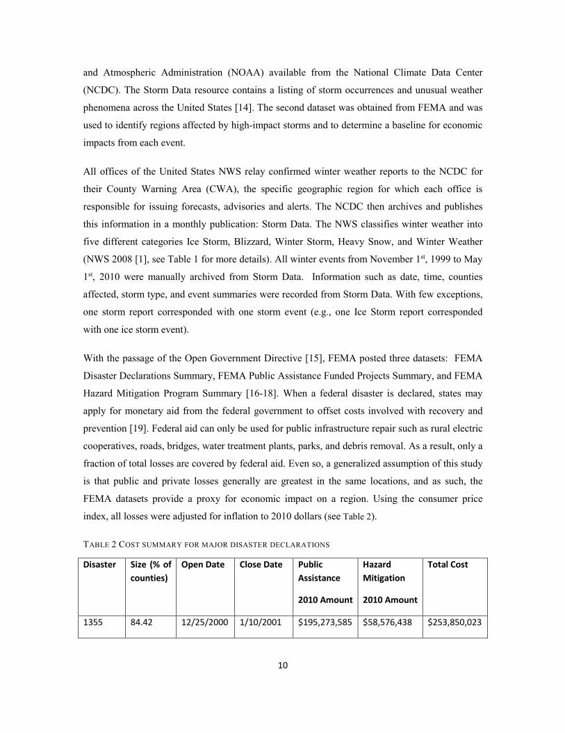
With the passage of the Open Government Directive [15], FEMA posted three datasets: FEMA

Disaster Declarations Summary, FEMA Public Assistance Funded Projects Summary, and FEMA

Hazard Mitigation Program Summary [16-18]. When a federal disaster is declared, states may

apply for monetary aid from the federal government to offset costs involved with recovery and

prevention [19]. Federal aid can only be used for public infrastructure repair such as rural electric

cooperatives, roads, bridges, water treatment plants, parks, and debris removal. As a result, only a

fraction of total losses are covered by federal aid. Even so, a generalized assumption of this study

is that public and private losses generally are greatest in the same locations, and as such, the

FEMA datasets provide a proxy for economic impact on a region. Using the consumer price

index, all losses were adjusted for inflation to 2010 dollars (see Table 2).

TABLE 2 COST SUMMARY FOR MAJOR DISASTER DECLARATIONS

Disaster Size (% of counties)

Open Date Close Date Public Assistance

2010 Amount

Hazard Mitigation

2010 Amount

Total Cost

1355 84.42 12/25/2000 1/10/2001 $195,273,585 $58,576,438 $253,850,023

10

Disaster Size (% of counties)

Open Date Close Date Public Assistance

2010 Amount

Hazard Mitigation

2010 Amount

Total Cost

1401 58.44 1/30/2002 1/11/2002 $135,435,131 $46,367,469 $177,802,600

1452 18.18 12/3/2002 12/4/2002 $5,142,582 $1,484,434 $6,627,016

1677 3.90 12/28/2006 12/30/2006 $7,131,386 $2,567,485 $9,698,871

1678 62.34 1/12/2007 1/26/2007 $82,643,557 $21,767,162 $104,410,720

1735 32.47 12/8/2007 1/3/2008 $103,873,997 $31,782,101 $135,656,098

1823 12.99 1/26/2009 1/28/2009 $9,479,711 $1,973,631 $11,453,341

1876 70.13 12/24/2009 12/25/2009 $18,063,800 $979,946 $19,043,746

1883 64.94 1/28/2010 1/30/2010 $75,457,829 $1,587,897 $77,045,726

Totals $628,501,577 $167,086,563 $795,588,140

FEMA disaster declarations summary. The Disaster Declarations Summary (Declaration)

dataset lists all declared major disasters since 1950. This dataset includes the unique disaster

number, dates of declaration, dates of incident, and names of counties affected.

FEMA public assistance funded projects summary. The Public Assistance Funded Projects

(PA) dataset lists all of the money disbursed by the federal government due to major disasters.

The PA funds offset costs to public property and interests, and do not include funds distributed by

private insurance companies. Further, the PA dataset lists federal aid disbursement by agency,

organization, declaration number, and county.

FEMA hazard mitigation program summary. The Hazard Mitigation Program (HM) dataset

lists money disbursed by FEMA to pay for projects that will help prevent future damages from

occurring. This dataset lists total costs of a project, location of project, and disaster number

associated with the project.

The three FEMA datasets were used to analyze spatial patterns of major disasters in Oklahoma, as

well as economic impacts on the state. Costs associated with the PA and HM datasets were

combined to determine the total public costs associated with the winter weather disasters during

this study. Because all of the data sources for this study reported locations by county, the spatial

11

resolution of this study is at the county level. There are several cases where funds, sometimes

considerable amounts, disbursed by the federal government were distributed statewide, as

opposed to an individual county. These statewide disbursements were omitted from the county

analysis, but were included when calculating overall total costs.

2.2 Results and Discussion 2.2.1 Storm Data Analysis The FEMA datasets demonstrated that nine major disasters were declared for Oklahoma due to

winter weather related conditions during the study period 2000 – 2010. In addition, the nine

declarations were the greatest number of any state in the United States during the period. The

counties with the most disaster declarations were oriented southwest to northeast and include

southwest, central, and northeast Oklahoma as shown in Figure 4 (a) Major disaster declarations (b)

total FEMA monetary aid (c) FEMA aid per capita

.

12

FIGURE 4 (A) MAJOR DISASTER DECLARATIONS (B) TOTAL FEMA MONETARY AID (C) FEMA AID PER CAPITA

13

FIGURE 5 TOTAL WINTER REPORTS 1 NOVEMBER 1999 - 1 MAY 2010 (A) AND POPULATION (B) FROM 2010 CENSUS

In terms of individual storm reports, from 2000 to 2010, the highest concentration of total winter

reports occurred in north central Oklahoma and the lowest concentration occurred in extreme

southern and southeastern Oklahoma (see Figure 5 Total winter reports 1 November 1999 - 1 May

2010 (a) and population (b) from 2010 census

14

). Biases in reporting, due to population, appears to be almost nonexistent as the correlation

between total storm reports and population yielded an R2 value of 0.01. For individual storm

types (Figure 6 Spatial distribution of storm types from 1 November 1999 - 1 May 2010

), Ice Storm reports were primarily concentrated in a southwest to northeast orientation, including

much of southwest, central, and northeast Oklahoma. This Ice Storm pattern was significant

because the state’s four most populous cities (Oklahoma City, Tulsa, Norman, and Lawton) were

located within this region. Heavy Snow was most frequently reported in the Oklahoma

panhandle while the Winter Storm category was most frequently reported in north central

Oklahoma. Blizzard reports, although few, were primarily located in the western half of

Oklahoma.

15

FIGURE 6 SPATIAL DISTRIBUTION OF STORM TYPES FROM 1 NOVEMBER 1999 - 1 MAY 2010

The patterns for Blizzard and Ice Storm reports, arguably the most severe winter storm types,

were spatially continuous throughout the study area. However, a reporting discontinuity between

NWS CWAs was evident between the Amarillo CWA and the Norman CWA for the Heavy Snow

and Winter Storm classifications. Another reporting discontinuity occurred as Winter Weather

reports were mostly confined to the Norman CWA and were virtually non-existent in both Tulsa

and Amarillo CWAs. To account for this pattern of reporting, all winter events (2000-2010) were

16

re-plotted without the Winter Weather reports to improve the overall consistency between NWS

CWAs.

The temporal analysis of the winter events during the study period revealed that December and

January received the most winter reports while the overall frequency of the reports were Winter

Storm (35%), Heavy Snow (26%), Ice Storm (16%), Winter Weather (20%), and Blizzard (3%).

For particular classifications, Ice Storms were most frequently reported in December, while

Winter Storm and Heavy Snow were most reported in December and January.

FIGURE 7 RATIO OF TOTAL WINTER REPORTS (MINUS WINTER WEATHER) TO MAJOR DISASTER DECLARATIONS

To better understand the frequency of these high impact winter events, total winter reports (minus

Winter Weather reports) were normalized with the number of major disasters declared (Figure 7

Ratio of total winter reports (minus Winter Weather) to major disaster declarations

). The results yielded that southwest Oklahoma had the lowest ratio of storm reports to disasters (as low as 2.2 storm events per declared disaster), while northwest Oklahoma had the highest ratio of storms to disasters (as high as 22 storm events per declared disaster). Overall, the minimum of storm reports to disasters was located in a southwest to northeast orientation across southwest, central, and northeast Oklahoma with much of southwest Oklahoma averaging three or less storm reports per declared disaster. Further, the ratio of Ice Storm reports during disaster declarations to total Ice Storm reports (Figure 8 Ratio of Ice Storm reports during disasters to total Ice Storm reports from 1 November 1999 - 1 May 2010

17

) demonstrated that at least 50% of the ice storm events yielded a disaster for nearly 70% of all Oklahoma counties (more than 80% of the population). Thus, while not as frequent, when ice storm events occurred they were usually associated with disaster related conditions over widespread regions that impacted significant portions of the population. By comparison, the ratio involving the combined Blizzard, Heavy Snow, and Winter Storm reports demonstrated that while such events often encompass large areas, generally less than 30% of the events would yield a disaster (Figure 8 Ratio of Ice Storm reports during disasters to total Ice Storm reports from 1 November 1999 - 1 May 2010

).

FIGURE 8 RATIO OF ICE STORM REPORTS DURING DISASTERS TO TOTAL ICE STORM REPORTS FROM 1

NOVEMBER 1999 - 1 MAY 2010

18

When considering total winter reports, one of the most noticeable patterns was the discontinuity

of reports between NWS CWAs. For example, the discontinuity was evident in the Heavy Snow

and Winter Storm reports and was especially noticeable with the Winter Weather reports. In this

case, the reporting discontinuity may be due to the preferences of the local NWS office. Given the

overlap of Heavy Snow and Winter Storm criteria it is possible that the Norman NWS office

prefers Winter Storm over Heavy Snow, especially because it is valid for multiple precipitation

types: snow for Heavy Snow and either snow or sleet for Winter Storm. Another possible reason

for the discontinuity of Winter Storm and Heavy Snow reports was based on the local, physical

conditions. The more frequent Heavy Snow reports in the Oklahoma panhandle may be due to a

common storm track known as the Panhandle Hook, a type of cyclone which develops in the

Oklahoma and Texas panhandle and typically deposits heavy snow just to the north of its track as

it moves northeast [20]. The higher elevations in the Oklahoma panhandle also contribute to more

frequent snow events as opposed to mixed precipitation events.

The specific discontinuity of Winter Weather reports also suggests a difference in reporting

preferences of the local NWS office. For this study, Winter Weather reports were virtually non-

existent in the Tulsa and Amarillo CWAs and were largely included within the Norman CWA.

Winter Weather reports typically reflect minor winter precipitation events and local NWS

forecast offices may not consistently report these low impact events. Branick [21] noticed

reporting inconsistencies in a nationwide study of Storm Data and concluded statewide

inconsistencies were possibly due to personnel at local NWS offices that have different standards

of reporting.

2.2.2 Climatological Trends Within broader climatological trends, the study period was characterized by an anomalously

greater number of significant winter-weather events. Changnon [4] showed that for Oklahoma

City (Oklahoma county in central Oklahoma), the two-year return period of a snow event was

approximately ten centimeters of snow. Over the study period (2000 – 2010) Oklahoma County

reported fifteen Heavy Snow and Winter Storm reports, each with a minimum threshold of ten

centimeters of snowfall. While the Winter Storm category could be reported solely because of

sleet, it is still reasonable that, many if not all Winter Storm reports met the snowfall criteria of

ten centimeters of snowfall. As such, Oklahoma City experienced a two-year event more than

once a year. Further, every county surrounding Oklahoma County also experienced at least ten

Heavy Snow and Winter Storm reports during the study period, which indicates that the local

region exceeded climatological norms for significant snowfall (2000 – 2010). 19

However, for all winter weather events, the results of this study noted that ice storms produce the

greatest frequency of disaster conditions. During the study period, such events were most

frequently reported in a southwest to northeast orientation across the central portion of the state.

Such occurrences were critical given that 80% of Oklahoma’s population resided in counties

which recorded four or more Ice Storm reports and over 40% of the population resided in

counties which recorded five or more Ice Storm reports.

Climatologically, the entire South category of the United States (including Oklahoma and

surrounding states) averages five to six catastrophic ( >$1 million) ice storms per decade [9].

Storm reports during all winter related disaster declarations [12] revealed that seven individual

counties within Oklahoma experienced four or more catastrophic ice storm events, during the

study period. As such, some individual counties in Oklahoma experienced nearly as many

catastrophic ice storms in the past decade as should impact a region that spans the entire South

category of the United States [9]. Further, Changnon [9] noted that over the period spanning the

period of 1949- 2000, the entire state of Oklahoma experienced eleven catastrophic ice storms or

approximately two per decade. Conversely, more than half of all Oklahoma counties experienced

between two and five catastrophic ice storms, measured by Ice Storm reports during disaster

declarations, through the study period (2000-2010).

Similar to Ice Storm reports, Blizzard reports were continuous across the state, further

demonstrating that the highest impact storms were consistently reported between NWS forecast

offices. Because Blizzards include wind criteria and climatologically stronger winds are located

across the western portion of the state [22], such reports were generally isolated to the western

half of Oklahoma. Schwartz and Schmidlin [23] analyzed blizzards across the United States from

1959 to 2000 and noted that during that 40-year period, only northwest Oklahoma experienced

any blizzards; approximately ten blizzards were reported in the Oklahoma Panhandle and up to

three in the northwest quarter of Oklahoma. However, from 2000 - 2010, the counties with the

most Blizzard reports were not located within the panhandle region, but across central and

southwest Oklahoma. Such results were significant given that the southwest quarter of Oklahoma,

a region which climatologically experienced no blizzards within the Schwartz and Schmidlin’s

study [23], had more Blizzard reports within the study period (2000 – 2010) than the entire forty

years previous (1959 – 2000). Further, when compared to the Schwartz and Schmidlin [23]

climatology, as many Blizzard reports occurred during the study period (2000 – 2010) over the

northwest quarter of Oklahoma as were recorded over the previous forty years (1959 – 2000).

20

2.2.3 FEMA Analysis Although Oklahoma typically experiences less winter storms than other regions of the United

States, the occurrence of high impact storms, as defined by disaster declarations, were numerous

during the study period. As such, with nine disasters statewide from 1 November 1999 – 1 May

2010, Oklahoma led the nation in winter weather related declarations and the areal coverage of

these events were large with the average winter related disaster encompassed approximately 45%

of the 77 counties in Oklahoma while the largest encompassed nearly 85% of all counties.

Further, over 60% of Oklahoma’s population resided in counties which had at least five

declarations during the study period and half of all Oklahoma counties were declared disasters at

least five times. Within a larger perspective, from 1 November 1999 to 1 May 2010, such

frequent local occurrences were greater than those for 43 entire states in the United States. The

total aid (PA & HM) allocated to the State of Oklahoma resulting from these disasters was

approximately 800 million USD (as shown in Table 2 Cost summary for major disaster declarations ).

The purpose for gauging high impact winter storms using disaster declarations (and allocated

Federal resources) is that it serves as a reliable proxy for estimating monetary damages associated

with these storms and associated socioeconomic impacts. While the total monetary disbursements

to Oklahoma from FEMA totaled near $800 million, the most populous counties, Oklahoma and

Tulsa counties, received the most monetary aid from the federal government, when compared to

other counties in the state. However, whereas 49% of Oklahoma’s population resides in five

counties (each with populations over 100,000 residents), these counties only accounted for 30%

of federal disbursements due to disasters. As such, 70% of federal funds were disbursed to the

remaining 72, more rural, counties (which included 51% of the population) during the winter

weather disasters. Thus, when associated disbursements were normalized to population, the

highest cost per capita occurred in rural counties outside of the main population centers.

Statistically, counties in the upper 50th percentile of disbursement per county (≥ $142 per capita)

accounted for 25% of the population and counties which had higher than the 75th percentile (≥

$284 per capita) accounted for only 10% of the population.

The allocation of federal resources in this manner demonstrates that although the most populous

counties received the greatest sum total of funds, the rural locales were most affected by the high-

impact winter storms and required more aid per given population base due to prolonged impact

on local infrastructure. The results are consistent with Call [24], who noted that rural regions are

more likely to suffer from prolonged power outages as utilities initially focus on regions with

higher numbers of customers. In addition, rural counties are less likely to have the resources 21

(personnel and updated technology) of more populated counties. Thus, when a wide-spread, high-

impact winter weather event occurs, rural areas require more external assistance than the local tax

base can accommodate.

For the study period, the highest cost per capita of federal funds due to disasters is located across

the southern half of Oklahoma, particularly southwest Oklahoma, which was also the region of

some of the lowest storm report per disaster ratios. As such, southwest Oklahoma, which was

largely rural, was particularly vulnerable to the frequent, high impact winter events that occurred

during the period and relied on increased external sources to assist the recovery.

2.3 Conclusion Oklahoma led the nation with nine winter related disaster declarations during the focus period of

this study (1 November 1999 – 1 May 2010) which accounted for nearly 800 Million USD in

total aid from the United States Federal Government. When compared with past climatological

analyses, the number and intensity of the high-impact winter weather events was anomalously

large across most of Oklahoma and particularly over southern and central portions of the state.

For example, central Oklahoma experienced, on average, a two-year snow event nearly every

year while southwest and central Oklahoma experienced as many as or more Blizzards during the

study period than over the previous forty-year period from 1959 – 2000 [23]. In addition, at least

half of all Oklahoma counties reached or exceeded the ten-year, statewide, climatological average

of catastrophic ice storms [9]. Such ice storm events were particularly devastating across much of

southern, central, and northeast Oklahoma and the results of this study demonstrated that

statewide approximately 50% of all Ice Storm reports occurred during disaster declaration

periods. Because the number of Ice Storm events was anomalously large and encompassed large

spatial areas during each event, the impacts frequently occurred in less prepared regions.

The devastating socioeconomic impacts of these winter weather disasters was, in part, revealed

by the federal aid distributed to regions across the state. The spatial distribution of the aid

revealed that, while the two most populous counties received the most monetary aid, overall the

rural counties (1) received the majority of federal aid from the disaster events and (2) yielded

greater per capita cost than the more populated counties. Thus, rural regions, with fewer resources

at their disposal, were more impacted by the high-impact winter weather events and required

more assistance from outside resources.

22

The contents of this section have appeared in, T. Grout, Y. Hong, J. Basara, B. Balasundaram, S.

T. S. Bukkapatnam and Z. Kong. Severe winter weather climatology and socioeconomic impact

in Oklahoma: 2000-2010. Journal of Weather, Climate, and Society, 2011, DOI 10.1175/WCAS-

D-11-00057.1.

23

3. Development and Implementation of a Storm Severity Index

During the past 50 years large-scale disruptions due to extreme winter weather events, especially

ice storms, have cost in excess of $45 billion on the nation’s infrastructure, and winter

maintenance approximately accounts for 25% of State Departments of Transportation (DOTs)

budgets [25]. Nationally, there have been 33 Presidential disasters declared because of snow and

ice since 2000 [12]. According to Federal Highway Administration (FHWA) statistics [26], State

and local agencies spend more than $2.5 billion on snow and ice control operations and more than

$5 billion to repair infrastructure damage caused by ice and snow. In the period of 1995–2004,

more than 389,000 crashes occurred in winter weather (6% of all crashes), more than 133,000

persons were injured in winter weather (more than 4% of all crash injuries) and more than 1,500

people were killed in crashes during winter weather (more than 3% of all crash fatalities).

Adverse weather is recognized as one of the leading causes of non-recurrent congestion, and in

particular winter precipitation alone can cause 15% of non-recurring delay. The cost of

congestion related travel delays on an economy is significant. It has been estimated that in

metropolitan areas, truckers lose about $3.4 billion (about 32 million hours) stuck in weather-

related traffic delays. A one-day highway shutdown can cost a metropolitan area up to $76

million in lost time, wages, and productivity [27]. Consequently, various state DoTs have been

striving for effective maintenance and response policies to mitigate hazard in the event of extreme

winter weather as part of their winter preparedness programs [28-33].

Weather data is essential to the decision making processes during severe winter weather. To make

effective decisions over large geographic regions, weather data must be gridded instead of point

based. To maximize preparedness, we need to forecast weather information (data) up to some

reasonable time scale into the future (2-3 days), which can be done through advanced weather

prediction models, such as the Weather Research and Forecasting model (WRF) and the Short

Range Ensemble Forecasting (SREF) model. Although these weather prediction models are ideal

for improving preparedness, they also require extensive background knowledge in meteorology to

be useful. It is important to present the model output clearly so that transportation managers can

focus on making decisions instead of learning those complex models. This goal can be

accomplished by developing winter severity indices tied to specific sectors of the economy.

There have been several indices developed recently and Maze et al. [34] contains a brief summary

of many of these. Many indices rank entire winter seasons using daily temperature and snow data

[35-37]. Some of these indices even factor in multiple precipitation types [38-40]. Nearly all of 24

these storm indices were developed using observed data and were applied to the entire winter

season. Maze et al. [34] notes a more recent index [41], which is storm based and includes factors

such as temperature, wind, and storm behavior. Other storm based indices have been developed

for specific types of precipitation such as the Nor’easter intensity index [42] or the Sperry-Piltz

[43] ice accumulation index which categorizes ice storms according to ice accumulation and

wind. Many of the existing indices are applied to winter seasons and not applied to individual

storms or they are based on observed data and not advanced numerical weather prediction

models. Furthermore, these indices are static and are not designed to be updated dynamically as

the storm data is gathered and forecasts are updated. Because winter storms affect different

sectors of the economy differently, it is important to tune an index to a specific sector. For

example, the Sperry-Piltz ice accumulation index applies to the electrical grid and utility

infrastructures and is hence used by utility managers. There are no known indices which utilize

advanced numerical weather prediction models and are tailored specifically to transportation

maintenance operations to classify individual storms.

3.1 Storm Severity Index Development A transportation-specific, storm-based, and dynamic Storm Severity Index (SSI), which accounts

for all major winter precipitation types (rain, snow, sleet, and freezing rain), was developed in

this study. It was designed to be compatible with multiple forecasting models such as the Weather

Research and Forecasting model (WRF) [44] or the Short-Range Ensemble and Forecast (SREF)

model [45]. Both of these models are advanced weather prediction models, which predict weather

conditions two to three days in advance. The WRF model has a higher resolution, more frequent

time steps and produces forecasts out of two days. The SREF is an ensemble model consisting of

over a dozen weather models and the mean of these models is used for the calculation of the SSI.

It has a coarser resolution compared to the WRF, but it forecasts for up to three days in advance.

Using weather parameters produced by weather prediction models, the SSI is specifically

formulated for transportation by accounting for precipitation intensity and visibility, precipitation

accumulation, as well as other non-precipitation hazards such as the winds, temperature, and

temperature trend. The SSI was developed similar to Boselly et al.’s work [36] with weather

parameters assigned categorical scores and then weighted relative to other parameters. The SSI is

composed of two sub-indices, which rate important non-precipitation parameters (Base Index)

and important precipitation parameters (Precip Index). The Base Index parameters are skin

temperature, temperature trend, and wind speed; while the Precip Index parameters are

precipitation impact on free flow traffic speed (a function of precipitation type, intensity, and 25

visibility) and precipitation accumulation. The total SSI is then the sum of both indexes. This SSI

is unique because it is a dynamic and gridded storm based index, which is tailored specifically to

transportation.

The SSI quantifies weather impacts on free flow traffic speed caused by both precipitation

intensity and precipitation accumulation. In addition, it can be used with multiple advanced

numerical weather prediction models (WRF or SREF), which can be used for both forecasting

and hindcasting purposes. Because this SSI is used with numerical weather models, it has the

same time step (typically 3 hours) and resolution (as low as 1km) as the weather prediction model

used. All parameters in both indices are divided into categories with each parameter category

assigned a score (from 0 to 1) based on severity. Additionally, each parameter is given a weight

(from 0 to 100%) so that they can be given a relative significance compared to other parameters

within each index. All parameter weights within an index must sum up to 100%, thus the index

score can have a maximum score of 100. The index score is the sum of the products of the

parameter’s categorical scores’ and that parameter’s weight. The mathematical formula (shown

as Eq. 1) for each index is represented as:

Index(maximum 100) = ∑[(Parameter category score ) × (Parameter Weight )] (1)

The SSI is only calculated during storm conditions, or when precipitation is forecast to begin until

24 hours after all precipitation has ended. Once a storm is over, the SSI is reset to zero and is not

calculated until precipitation is predicted to begin again. The 24 hour period assumes that the

emergency response to high-impact winter storms will be completed within 24 hours after the last

predicted winter precipitation falls.

3.1.1 Base Index The first index is the Base index (see Table 3 Base index description , adapted from Kyte et al. [46],

who quantified wind effects on driving conditions in free flow speed), which consists of three

important non–precipitation parameters (surface temperature, temperature trend, and wind speed)

that impact winter storm severity.

TABLE 3 BASE INDEX DESCRIPTION

Index Parameter Weight (%) Score (0 - 1)

BA

SE

Temperature 40 Above Freezing (1), Below Freezing (0)

Temperature Trend 10 Increasing (0), Decreasing (1)

26

Index Parameter Weight (%) Score (0 - 1)

Windspeed1 50

Windspeed < 10 mph (0); 16mph ≤ Windspeed ≤ 20 mph (0.33) 20 mph < Windspeed ≤ 30 mph (0.66)

Windspeed > 30 mph (1)

Surface temperature is important because it is the ground temperature and thus the closest

approximation to the pavement temperature. Temperature trend is important because it indicates

if the temperature is decreasing (more severe) or increasing (less severe). Finally, wind speed is

included because it can influence traffic conditions as velocities increase. Calculation of the base

index involves assigning a score to each weather parameter (between 0 and 1) as well as a

parameter weight (summed to 1) (see Figure 9 Flowchart for Base Index: Base index score is

calculated by multiplying the parameter weight with the parameter score. Max score is 100.

for details).

3.1.2 Precip Index The Precip index (see Figure 10 Flowchart for Precip Index: Precip index score is calculated by

multiplying the parameter weight with the parameter score. Max score is 100.

) consists of important precipitation based parameters and their impact on transportation. The

first parameter is storm total precipitation accumulation. Precipitation accumulation severity is

dependent upon the precipitation type; one inch of snow is not as severe as one inch of ice. The

second parameter describes the impact of precipitation on free flow traffic speed. This parameter

incorporates precipitation type, intensity and visibility, and quantifies the impact on traffic flow.

The Precip index consists of two parameters: precipitation accumulation and precipitation

intensity effect on free flow traffic speed. The scores and weights assigned each parameter are

explained in the following.

Precipitation Accumulation: Accumulation scores were adapted or slightly modified from Nixon

and Qiu [41], who quantified the relative impact of winter storm accumulations on transportation

for different precipitation types. All precipitation estimates are calculated using liquid equivalent

amounts. All freezing rain amounts are radial equivalent accumulations according to the method

described by Jones [47]. Snow and sleet amounts were derived using general conversions from

liquid equivalent amounts [48, 49].

27

FIGURE 9 FLOWCHART FOR BASE INDEX: BASE INDEX SCORE IS CALCULATED BY MULTIPLYING THE PARAMETER WEIGHT WITH THE PARAMETER SCORE. MAX SCORE IS 100.

28

FIGURE 10 FLOWCHART FOR PRECIP INDEX: PRECIP INDEX SCORE IS CALCULATED BY MULTIPLYING THE PARAMETER WEIGHT WITH THE PARAMETER SCORE. MAX SCORE IS 100.

Precipitation impact on Free Flow Traffic Speed: This parameter incorporates precipitation

intensity and visibility. Categories for this parameter are numerous but they are all based upon

visibility, intensity, and precipitation type. This parameter is weighted more than accumulation as

precipitation intensity is more impactful on transportation than storm accumulations.

Snow and Sleet: Snow and sleet have the highest impact on visibility. Average liquid-equivalent

hourly snowfall/sleet rates are calculated from model output and intensities are assigned

according to Rasmussen and Cole [50]. Visibility (a function of precipitation intensity),

temperature, and time of day, were assigned according to Rasmussen and Cole [50]. Rakha et al.

[51] studied how precipitation impacts free-flow traffic speed; it is a function of precipitation

intensity and visibility. Intensities and visibilities determined from Rasmussen and Cole [50]

were applied to Rakha et al [51] to determine the impact of precipitation intensity on free flow

traffic speed. Scoring was the ratio of the impact on free-flow traffic speed to the maximum

possible impact on free-flow traffic speed.

Rain/Freezing Rain: According to Rassmussen and Cole [50], liquid precipitation does not

impact visibilities near as much as snowfall. Rakha et al. [51] does quantify rainfall intensities on

free flow traffic speed. Unfortunately, freezing rain’s impact on free flow traffic speed is not well 29

studied and accurate impacts on free flow traffic speed are not available. To account for freezing

rain it was assumed that for any three hour period, or time step of the model, if a location was

forecast to experience freezing rain with radial ice accumulations greater than .01” then that

location would receive a maximum score of 1. This may be excessive, but the impact of freezing

rain cannot be overemphasized.

3.2 SSI Implementation and Preliminary Evaluation The SSI is implemented over the winter seasons of 2000-2010. A WRF model was run in-house

for all winter seasons (December to March) from 2000- 2010 for central Oklahoma. SSI scores

for each grid were accumulated on a 12 hourly and daily basis and they yielded a log-normal

distribution (see Figure 11 and Figure 12). In addition, a statewide WRF model was run for some

major disaster storms of the past decade in Oklahoma.

FIGURE 11 LOG SSI DISTRIBUTION ON A 12 HOUR BASIS

To evaluate the SSI, daily accident data including injuries and fatalities, for Oklahoma county for

10 winter months (from 2000 – 2010) was obtained from the Oklahoma Department of

Transportation [52]. These accident statistics spanned some of Oklahoma’s most severe winter

weather including many of the winter related major disasters. A statistical validation of the SSI is

underway at the time of this writing and is expected to be a part of a future research publication

that is planned, based on this work.

30

FIGURE 12 LOG SSI DISTRIBUTION OF SSI SCORES ON A DAILY BASIS

3.3 Conclusion A storm severity index was developed geared specifically toward transportation. The SSI

provides a user-friendly approach to enable transportation officials to be better informed with

regards to impending winter weather. This approach is an improvement over other severity

indices because it is transportation specific, storm based, and it is both (spatially) gridded and

dynamic. The SSI incorporates multiple weather parameters that influence transportation safety.

In addition, using advanced weather prediction models enables the SSI to be calculated for both

past and present winter events. By using a gridded and predictive SSI, transportation planning

managers can anticipate severe winter weather and specifically its potential impact on

transportation infrastructure. In rapidly changing weather conditions, as the weather models

update, SSI can also be updated dynamically. As weather prediction models improve in accuracy

so will the SSI. The SSI shows some preliminary statistical evidence of being a better indicator of

transportation specific storm severity than simpler indicators like predicted snow/ice thickness or

precipitation depth alone. The results of this research are currently being prepared for

publication.

31

4. Nonlinear Bayesian Analysis for Snow/Ice Thickness Prediction

Predicting weather parameters including ice/snow thickness is key to accurately forecasting SSI

and it is also needed in the stochastic optimization model for maintenance resource allocation.

The methodological contributions in this regard are detailed in this section. These numerical

prediction models are complementary to WRF/SREF models employed in the development of SSI

as they offer higher resolution, are relatively easier to work with from a computational

perspective, and enable probabilistic forecasts as opposed to point estimates of weather

parameters, when compared to WRF/SREF models that employ physics models and need

supercomputing resources.

Probabilistic forecast of weather parameters has many advantages over the non-probabilistic

forecast techniques in aiding weather related decision making processes [53]. An emergency

manager can better decide whether to use anti-icing treatments or de-icing treatments based on

the probability of icing on the road. Physical forecast models do not consider uncertainties in both

initial conditions and model formulation [54], a drawback that can be addressed by probabilistic

models. Previous research shows that, decision-makers provided with information about

uncertainty can make better decisions compared to those who do not have this information [55].

In addition, classifying storms into different categories in terms of their severity is essential for

the optimization based resource allocation decision support system. In order to classify upcoming

storms, we need accurate forecast of weather parameters. In this study we develop such a

probabilistic forecast system that incorporates outputs of physical models and historical data.

4.1 Literature Review Time series models such as autoregressive moving average (ARMA) models are widely used in

weather forecasting. ARMA models assume a linear relationship between current data and past

data. While they are effective for stationary and linear systems, they are not best suited for

predicting weather parameters. ARMA models use iterative methods to find the optimal model

parameters which makes them computationally demanding. For example, an ARMA model is

constructed by Torres et al. to forecast short term average wind speed in [56]. To overcome the

challenge of seasonality difference in their study, ARMA models are developed for each month.

Burlando et al. [57] employed ARMA models for rainfall forecasting by investigating all rainfall

occurrences in a period and using an event based approach.

32

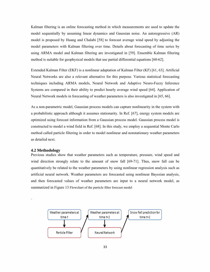
Kalman filtering is an online forecasting method in which measurements are used to update the

model sequentially by assuming linear dynamics and Gaussian noise. An autoregressive (AR)

model is proposed by Huang and Chalabi [58] to forecast average wind speed by adjusting the

model parameters with Kalman filtering over time. Details about forecasting of time series by

using ARMA model and Kalman filtering are investigated in [59]. Ensemble Kalman filtering

method is suitable for geophysical models that use partial differential equations [60-62].

Extended Kalman Filter (EKF) is a nonlinear adaptation of Kalman Filter (KF) [61, 63]. Artificial

Neural Networks are also a relevant alternative for this purpose. Various statistical forecasting

techniques including ARMA models, Neural Network and Adaptive Neuro-Fuzzy Inference

Systems are compared in their ability to predict hourly average wind speed [64]. Application of

Neural Network models in forecasting of weather parameters is also investigated in [65, 66].

As a non-parametric model, Gaussian process models can capture nonlinearity in the system with

a probabilistic approach although it assumes stationarity. In Ref. [67], energy system models are

optimized using forecast information from a Gaussian process model. Gaussian process model is

constructed to model a wind field in Ref. [68]. In this study, we employ a sequential Monte Carlo

method called particle filtering in order to model nonlinear and nonstationary weather parameters

as detailed next.

4.2 Methodology Previous studies show that weather parameters such as temperature, pressure, wind speed and

wind direction strongly relate to the amount of snow fall [69-71]. Thus, snow fall can be

quantitatively be related to the weather parameters by using nonlinear regression analysis such as

artificial neural network. Weather parameters are forecasted using nonlinear Bayesian analysis,

and then forecasted values of weather parameters are input to a neural network model, as

summarized in Figure 13 Flowchart of the particle filter forecast model

.

33

FIGURE 13 FLOWCHART OF THE PARTICLE FILTER FORECAST MODEL

During severe storm conditions, weather parameters changes rapidly. Thus, we need to run the

physical models frequently to get accurate forecast. Because physical models are

computationally intensive, it is not preferable to use them for short term forecasting. Statistical

methods can be useful since they are fast and accurate. WRF model itself for example uses

Gaussian process models for statistical forecasting. While they can handle the nonlinearity well,

Gaussian assumption restricts its application in the forecasting of weather data. In addition,

Gaussian process model assumes stationarity (the covariance structure is time independent),

which may not hold under storm conditions. In order to address this problem, a sequential Monte

Carlo method, namely Particle Filtering (PF) is utilized in this study to forecast the weather

parameters. PF method is also compared against other widely used techniques, including Kalman

filtering (KF) and Gaussian Process.

In order to demonstrate the advantage of particle filtering model over Kalman filtering and

Gaussian process, the models are applied to temperature data for one-hour ahead forecasting as

shown in Figure 14 Comparison of various forecasting methods for one-step ahead temperature

prediction

. The data is obtained from MESONET [72]. The accuracy of the different methods, defined in

Eq. 2 (also known as R2), is compared in

34

FIGURE 14 COMPARISON OF VARIOUS FORECASTING METHODS FOR ONE-STEP AHEAD TEMPERATURE PREDICTION

Accuracy = (1− Mean Square ErrorVariance of Data

) × 100 (2)

TABLE 4 ACCURACY OF DIFFERENT FORECASTING METHODS

FORECASTING METHOD ACCURACY (R2)

KALMAN FILTER 78.56%

GAUSSIAN PROCESS 86.37%

PARTICLE FILTER 92.35%

In addition to air temperature (at the height of 1.5 m), relative humidity, solar radiation, air

pressure, average wind speed, wind direction, temperature (at 9 m) parameters are also forecasted

in order to predict snow fall. Figure 15 One Step Ahead Forecast of Relative Humidity (%) (top) and

Solar Radiation W/m2 (bottom)

, Figure 16 One Step Ahead Forecast of Air Pressure (mbar)(top) and Air Temperature at 9 m 35

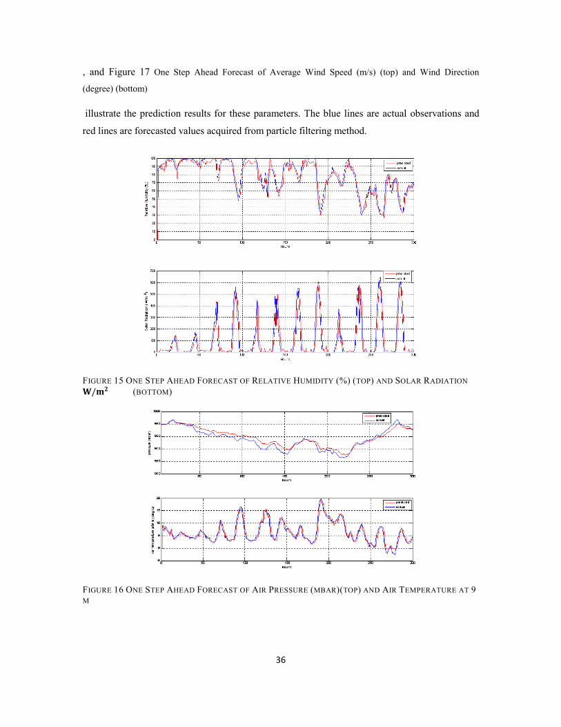
, and Figure 17 One Step Ahead Forecast of Average Wind Speed (m/s) (top) and Wind Direction

(degree) (bottom)

illustrate the prediction results for these parameters. The blue lines are actual observations and

red lines are forecasted values acquired from particle filtering method.

FIGURE 15 ONE STEP AHEAD FORECAST OF RELATIVE HUMIDITY (%) (TOP) AND SOLAR RADIATION 𝐖𝐖/𝐦𝐦𝐦𝐦 (BOTTOM)

FIGURE 16 ONE STEP AHEAD FORECAST OF AIR PRESSURE (MBAR)(TOP) AND AIR TEMPERATURE AT 9 M

36

FIGURE 17 ONE STEP AHEAD FORECAST OF AVERAGE WIND SPEED (M/S) (TOP) AND WIND DIRECTION (DEGREE) (BOTTOM)

TABLE 5 ACCURACY RESULTS FOR FORECAST OF WEATHER PARAMETERS

Weather Parameter Accuracy (R2)

Relative Humidity 91.36%

Solar radiation 86.32%

Air Pressure 88.24%

Air Temperature (at 9m) 92.25%

Average Wind Speed 89.58%

Wind Direction 87.46%

Table 5 shows R2 values for one step ahead forecasting of different weather parameters by using

particle filtering. All the values are above 85% accuracy which can be used for accurate snow

depth prediction.

4.3 Predicting Snow Depth Using Artificial Neural Networks After the prediction of the weather parameters (relative humidity, solar radiation, air pressure,

average wind speed, wind direction, temperature) using particle filtering method, these are input

to a neural network model to predict snow/ice thickness, as illustrated in Figure 18 Flowchart for

snow depth forecasting using the predicted weather parameters

.

37

FIGURE 18 FLOWCHART FOR SNOW DEPTH FORECASTING USING THE PREDICTED WEATHER PARAMETERS

A feed forward neural network with 2 layers and 20 neurons is used for snow depth prediction.

Out of 130 data points; 64 data points are used for training, 33 used for validation and 33 used for

testing. Prediction accuracy of snow depth is 80%. Comparison of observation and prediction of

the snow depth is illustrated in Figure 19 Comparison of observation and prediction of the snow depth

using Neural Network model

, which indicates the high accuracy of the neural network model.

FIGURE 19 COMPARISON OF OBSERVATION AND PREDICTION OF THE SNOW DEPTH USING NEURAL NETWORK MODEL

4.4 Conclusion This section surveyed various numerical prediction models available in the literature, specifically

ones used to predict weather parameters. A particle filter method is developed to predict several

weather parameters that are subsequently used in the prediction of snow/ice thickness using an

artificial neural network. Preliminary experiments indicate that this technique is better suited to

predict nonlinear and nonstationary weather parameters and snow/ice depth frequently over short

ranges with reasonable computational effort. The parameters predicted using the particle filter 38

method and the snow/ice depth predictions using the neural network model are used in the SSI

model to predict the SSI for future time periods during a storm event, which is used subsequently

in the stochastic optimization model for resource allocation.

39

5. Optimization Model for Resource Allocation and Risk Mitigation

In the United States, winter road maintenance (WRM) operations take up significant portion of

annual operating budgets in many states [73]. Under severe winter weather, the State DOTs are

typically responsible for different transportation risk mitigation activities such as plowing

(removal of snow and ice from the road using specially equipped trucks), anti-icing (preventing

ice formation on the road by treating with sodium chloride or rock salt, other compounds such as

calcium chloride, magnesium chloride are also used combined with road-bonding agents to

enhance corrosion inhibition properties), de-icing (if ice forms on the road, it is treated with

chemicals to keep it from compacting and bonding to the road surface, this facilitates plowing),

and spreading abrasives (chemically wetted sand is spread at turns, intersections, gradients on the

road to improve traction). The State DOT's responsibilities during emergencies may also include

moving power generators to hospitals and other critical places that are suffering from power

outage, restoring utility poles that are down, moving potable water in tankers to small towns

where water supply has been cut-off due to utilities being incapacitated, removing debris in the

wake of ice storms, setting up portable message boards warning commuters of frozen roads or

other hazards as they develop.

Clearly, the maintenance operations are complicated, and their effectiveness depends on the

availability of appropriate resources at the appropriate time and place, which in turn is

complicated by the uncertainty in the severity of the winter storm hazard in addition to resource

and capacity limitations. The maintenance resource allocation decisions have to be made under

limited capacity/resource availability, and uncertain information, and needs to be done a priori to

allow the development of a maintenance operational plan. It is hence, important to employ a

suitable optimization model that captures uncertainty and resource limitations, with an objective

which drives decisions leading to a desirable system behavior. We discuss some relevant

concepts prior to developing such a mathematical model in Section 5.2.

5.1 Hazard, Vulnerability and Risk Vulnerability analysis deals with the ``cost of an emergency,'' that is, the value of service

provided by the transportation system, or infrastructure. In contrast, hazard analysis deals with the

“likelihood of an emergency.” Risk, is the probability that more than a threshold level of service-

reduction is sustained by a transportation system, or infrastructure. That is, risk is a measure of

combined effects of vulnerability and hazard probability. Consider the following examples for

illustration purposes. Suppose a segment of a bridge is missing due to construction delays. This is 40

poses a hazard- certain catastrophe for any traffic ``on that segment.'' If this bridge is closed to

traffic, there is no service provided and hence, it is not vulnerable. Thus, a hazardous highway

segment poses no risk, if it is closed for service. On the other hand, consider a major highway

segment that serves a large volume of traffic, hence, it is a vulnerable asset. It would be

considered hazardous if its structural integrity is questionable, and it would then be considered

risky. If it is reinforced structurally, it is less hazardous and hence, it becomes less risky, even

though it is still equally vulnerable. If traffic flow is reduced by newly developed alternate routes,

this highway segment is less risky as it is now less vulnerable, although it is equally hazardous.

The importance of a particular link in a road network is measured as the normalized freight plus

passenger flow (rate) on the link, which can either be obtained directly from public databases or

by heuristically solving a freight flow assignment model. We use a heuristic approach to flow

assignment, illustrated in

Figure 20 Heuristic algorithm for freight flow assignment

, developed as a part of the Freight Movement Model project completed recently by Drs. Kamath

and Ingalls at OSU in collaboration with OU. Implementation of this heuristic using the

mathematical programming solver IBM ILOG CPLEX® was completed and another

implementation based on our implementation of Dijkstra’s algorithm was also completed, which

was found to scale better than CPLEX given the massive size of the US highway network under

41

consideration. Hence, we further improved the Dijkstra implementation by employing some well-

known graph libraries that implement the algorithm using more sophisticated data structures.

FIGURE 20 HEURISTIC ALGORITHM FOR FREIGHT FLOW ASSIGNMENT

5.2 Optimization of Conditional Value-at-Risk (CVaR) The modeling approach employed in this study is the optimization of Conditional Value-at-Risk

(CVaR). Rockafellar and Uryasev pioneered the work [74, 75] on developing the general

methodology of optimization of CVaR and applying it to portfolio optimization problems. The

notion of Value-at-risk (VaR) is well-known in financial applications, and the related notion of

CVaR as a downside measure of risk is fast gaining acceptance in finance due its many desirable

properties. In this study we develop CVaR optimization models to identify maintenance resource

allocation decisions that minimize the risk of high-losses under probabilistic storm severity

information.

The general framework is as follows. Assume, that L(x,Y) is the loss in a system associated with

the decision vector x and the random vector Y representing uncertain parameters involved in the

operations of a system. In our case, x represents the resource allocation decisions and y is a vector

of random variables indicating the severity of the storm event. For each x, the loss L(x,Y) is a

random variable having a distribution induced by that of Y. However, an analytical expression the

loss distribution is not needed for the implementation of this approach.

42

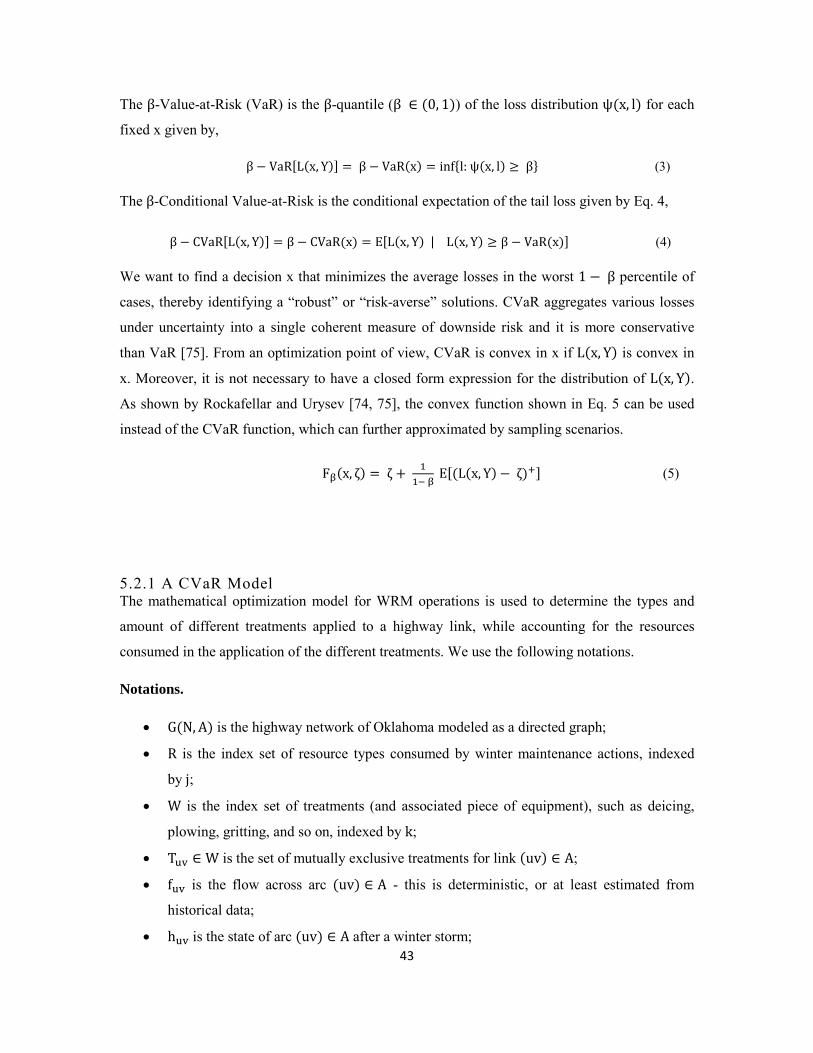
The β-Value-at-Risk (VaR) is the β-quantile (β ∈ (0, 1)) of the loss distribution ψ(x, l) for each

fixed x given by,

β − VaR[L(x, Y)] = β − VaR(x) = inf{l: ψ(x, l) ≥ β} (3)

The β-Conditional Value-at-Risk is the conditional expectation of the tail loss given by Eq. 4,

β − CVaR[L(x, Y)] = β − CVaR(x) = E[L(x, Y) | L(x, Y) ≥ β − VaR(x)] (4)

We want to find a decision x that minimizes the average losses in the worst 1 − β percentile of

cases, thereby identifying a “robust” or “risk-averse” solutions. CVaR aggregates various losses

under uncertainty into a single coherent measure of downside risk and it is more conservative

than VaR [75]. From an optimization point of view, CVaR is convex in x if L(x, Y) is convex in

x. Moreover, it is not necessary to have a closed form expression for the distribution of L(x, Y).

As shown by Rockafellar and Urysev [74, 75], the convex function shown in Eq. 5 can be used

instead of the CVaR function, which can further approximated by sampling scenarios.

Fβ(x, ζ) = ζ + 11− β

E[(L(x, Y)− ζ)+] (5)

5.2.1 A CVaR Model The mathematical optimization model for WRM operations is used to determine the types and

amount of different treatments applied to a highway link, while accounting for the resources

consumed in the application of the different treatments. We use the following notations.

Notations.

• G(N, A) is the highway network of Oklahoma modeled as a directed graph;

• R is the index set of resource types consumed by winter maintenance actions, indexed

by j;

• W is the index set of treatments (and associated piece of equipment), such as deicing,

plowing, gritting, and so on, indexed by k;

• Tuv ∈ W is the set of mutually exclusive treatments for link (uv) ∈ A;

• fuv is the flow across arc (uv) ∈ A - this is deterministic, or at least estimated from

historical data;

• huv is the state of arc (uv) ∈ A after a winter storm; 43

• ρuvk is the percentage improvement in condition that treatment k ∈ W restores to link

(uv) ∈ A;

• ruvjk is the amount of winter road maintenance resources of type j ∈ R consumed by one

unit of WRM equipment or crew for treatment k ∈ W on link (uv) ∈ A. If resource j ∈ R

is not used for treatment k ∈ W, then ruvjk = 0;

• rtotj is the total amount of resource j ∈ R currently in inventory;

• uj is the upper bound on the amount of resource j ∈ R available for purchase;

• Cuvk is the cost per unit of equipment to apply treatment k ∈ W to arc (uv) ∈ A;

• dj is cost to buy or rent one unit of resource j ∈ R;

• b is the total budget;

• muvk is the maximum units of treatment k ∈ W that can be applied to link (uv) ∈ A;

• S is the index set of scenarios, indexed by s;

• huvs is the condition of link (uv) ∈ A in scenario s ∈ S;

• β is the percentile of the loss distribution;

• 𝑝𝑝𝑠𝑠 is the probability of scenario 𝑠𝑠 ∈ 𝑆𝑆

• [θ]+ = max (0,θ).

Decision variables.

• xuvk is the units of WRM treatment k ∈ W applied to arc (uv) ∈ A;

• wuvk is 1 if treatment k ∈ W is applied to arc (uv) ∈ A, and 0 otherwise.

Loss function.

Loss function that is used in this model is described according to Eq. 6.

L(x,ℎ𝑠𝑠) = ∑ fuv�huvs − ∑ ρuvk xuvkk∈W �+(uv)∈A (6)

Model.

Minimize ζ + 11− β

[∑ 𝑝𝑝𝑠𝑠𝑠𝑠 ∈𝑆𝑆 (𝐿𝐿(𝑥𝑥,ℎ𝑢𝑢𝑢𝑢𝑠𝑠 )− ζ)+]

Subject to:

44

� � ruvjk xuvk

(uv)∈Ak∈W

≤ rtotj + uj ∀j ∈ R (7)

� � Cuvk xuvk(uv)∈A

+ �dj �� ruvjk xuvk − rtot

j

(uv)∈Ak∈W

�

+

j∈Rk∈W

≤ b (8)

xuvk ≤ muvk wuv

k ∀(uv) ∈ A, k ∈ W (9)

� wuvk ≤ 1 ∀(uv) ∈ A

k∈Tuv

(10)

xuvk ≥ 0 and integer; wuvk ∈ {0,1} ∀(uv) ∈ A, and k ∈ W (11)

Constraint (7) indicates that the amount of resources used should not exceed availability,

including what is immediately available and what can be purchased or rented. Constraint (8)

ensures that all expenditures are less than the total budget. Constraint (9) states that each link

cannot get assigned more units than the maximum that can be allocated to that link. Constraint

(10) ensures that at most one kind of treatment among the group of mutually exclusive treatments

associated with a link can be used on that link.

5.3 Results from Numerical Experiments This model was implemented in C++ using IBM ILOG CPLEX® libraries for solving the mixed

integer optimization problem. The experiments were conducted on a Windows XP PC with 2.26

GHz i3 CPU and 4.00 GB of RAM. The following combination of real-life data and synthetic

data was used in our preliminary experiments to validate this proof-of-concept model.

• Highway network of Oklahoma

• Vulnerability of links measured as annual average daily traffic flow rates

• Amount of resources used by each treatment.

• Maximum available amount of resources and maximum amount can be rented.

• Unit cost to apply each treatment.

• Unit cost to rent each resource.

• Percentages of improvement when one unit of each treatment is applied to a link.

Table 6 Amount of resources used by each treatment - Table 10 show the synthetic data that was

generated for experimental purposes.

45

TABLE 6 AMOUNT OF RESOURCES USED BY EACH TREATMENT

Resource 1 Resource 2 Resource 3 Resource 4 Resource 5

Treatment 1 2 3 2 0 3





TABLE 7 MAXIMUM AMOUNT OF RESOURCES AVAILABLE

Resource number In inventory Available to rent

1 50000 50000

2 20000 80000

3 60000 40000

4 80000 20000

5 40000 60000

TABLE 8 UNIT COST TO APPLY EACH TREATMENT

Treatment number Costs

1 200

2 180

3 300

4 80

5 120

TABLE 9 UNIT COST TO RENT EACH RESOURCE

Resource number Costs

1 250

46

Resource number Costs

2 210

3 380

4 140

5 150

TABLE 10 PERCENTAGE IMPROVEMENT FROM UNIT APPLICATION OF A TREATMENT

Treatment number % improvement

1 5

2 10

3 8

4 9

5 10

The Oklahoma highway network and traffic flow data used in our experiments was obtained from

the Freight Analysis Framework database maintained by the Federal Highway Administration. It

has 2806 nodes, and we only consider class 1, class 2, and class 3 highways resulting in 3303

links. This corresponds to an optimization model with 198, 236 decision variables and 350, 179

constraints and solving this model to optimality takes more than 1 hour. So, we terminate the

algorithm when the optimality gap (tolerance) reduced below 10%, which happens in under 400

seconds. Another aspect of solving this problem concerns scenario generation or sampling. We

solved the model with 50 scenarios generated by particle filtering, discussed in Section 4.

Particle filtering gives us probability of each weather parameters at time (t+s) given those at time

t. Then forecasted weather parameters are plugged into the SSI model discussed in Section 3 to

predict SSI values at the time (t+s). This process was repeated for all 120 mesonet stations in

Oklahoma and 100,000 scenarios are randomly generated. From these 100,000 randomly

generated scenarios, 50 scenarios with the highest probability were selected. Finally, the

probabilities were normalized to ensure that the summation of probabilities for all 50 scenarios is

equal to 1.

47

The goal of this model is to improve the link conditions under uncertain severe winter weather by

allocating maintenance resources to minimize the conditional-value-at-risk of losses. Figure 21

Vulnerability analysis before assignment

and Figure 22 Vulnerability analysis after assignment

48

illustrate the link conditions before and after assignment respectively. That is, comparing the

performance of the solution found by the model against the same CVaR objective when no

resources are allocated. This is an extreme comparison, however, it does provide a baseline for us

to assess the extent of the impact in the absence of any treatment, to the one recommended by the

model. One of the future tasks is to validate the model and its performance against simple greedy

heuristics that mimic the decision making process of a maintenance manager in the absence of

any sophisticated mathematical model to aid their decisions. As shown in Figure 21 Vulnerability

analysis before assignment

and Figure 22 Vulnerability analysis after assignment

49

, before assignment, flows on almost all links are reduced by more than the Beta value (0.95) due

to severe weather. But after assignment, link conditions are improved for most of the links.

FIGURE 21 VULNERABILITY ANALYSIS BEFORE ASSIGNMENT

FIGURE 22 VULNERABILITY ANALYSIS AFTER ASSIGNMENT

50

6. Deliverable: Prototype DSS Implementation The technical results and conlusions from the SSI model, prediction models and the CVaR

optimization model were discussed at the end of the respective sections. However, the overall

goal of this two year project was the development of a prototype DSS that combines each module

(SSI, prediction and optimization) into a single user-friendly interface along with pertinent data,

to generate visualizations and other numerical outputs that aid a maintenance manager. We

conclude this report with a discussion of such an implementation which is available upon request

from the research team. The DSS developed is a proof-of-concept demonstrating the feasibility of

integrating sophisticated mathematical models into a system that enables informed decision-

making. Our results demonstrate the potential advantages of developing our research results into

professional software packages that ODOT could employ.

The prototype DSS is called the Winter Resource Allocation & Maintenance: Decision Support

System (WinRAM DSS) and it has been implemented using Microsoft Visual Studio® and it

utilizes Matlab®, and IBM ILOG CPLEX® optimization engine for its various functions.

Visualization is done using the GIS software TransCAD®. WinRAM DSS has four tabs, namely,

SSI Analysis tab, Prediction Model tab, Optimization Model tab, and an About tab. All SSI

analysis, prediction model and optimization model tabs follow the same input procedure. They

read information from a working folder, set the parameters, check all input files, run models, and

visualize results. Also in those tabs, you can copy some files from another folder to the working

folder, if it is needed. This was done to faciliate “what-if” analyses where different what-if test

cases stored in different folders are automatically copied into the working folder with a single

button click to make them easier to run.

6.1 SSI Analysis Tab SSI Analysis tab can be used to generate color-coded maps of SSI for different storms including

future storms, based on the forecasts. To generate the color maps, two models (SREF or WRF)

are used. After a model is chosen, the date of the storm event must be chosen. After a model is

chosen, the event for that model will be shown in a drop-down box and other inapplicable events

are deactivated. Other inputs for the SSI model are accumulation and quantile. Both precipitation

accumulation and intensity are used to calculate the SSI, and the relative weights of their

importance must be provided. Default is 30% for accumlation with intensity accounting for 70%.

This is useful as sometimes intensity is more important, for example when if there is a heavy

snow squall which is brief but very intense. The accumulation would not be very significant but

the intensity would be very important as it would impact transportation. The quantile is provided 51

so that the SSI quantile score at three hour intervals can be generated for every event. The

median and maximum SSI are especially useful to see how severe the storm is on average and

how intense the storm will be at its worst. After all input files are confirmed, a chosen model can

be run. Outputs can be shown in detail or summary. The detailed plot output is a three hour SSI

model for the entire event. The summary plot is a quantile summaries for the entire storm.

Screenshot of the SSI tab is given in Figure 23 and a sample output from running the SSI model

with SREF is shown in Figure 24 for illustration purposes.

FIGURE 23 SSI TAB SCREENSHOT

FIGURE 24 SSI OUTPUT ILLUSTRATION

52

6.2 Prediction Model Tab The Prediction tab can be used to access and run the models for forecasting the weather

parameters, including temperature, relative humidity, wind speed and air pressure. The predicted

weather parameters are then used to calculate SSI as discussed in the previous section. The

weather condition as quantified by the SSI is separated into three classes, namely, low, medium

and severe. The probabilities of belonging to different categories are illustrated as color-coded

map throughout the state of Oklahoma. Predicted weather parameters are also used to generate

visualizations.

Particle filtering technique is employed here for the weather parameters forecasting. Historical

data files are extracted directly from MESONET website [72] which allows us to update the

model dynamically. The DSS requests two input parameters (number of particles, noise level)

from the user. Large number of particles can better approximate the distribution of weather

parameters, which can improve forecasting accuracy, but requires more computational effort.

There is a trade-off between computational time and accuracy controlled by the number of

particles chosen. The default particle number value is set as 100.

Second parameter is the noise level, which is relates to data quality. Especially during severe

weather conditions, the quality of data collected is questionable as the measurements under these

conditions may no longer be as reliable, requiring us filter out the noise in data. The default value

for noise level is set at 0.01 which means that 1% of data is assumed to be noise.

Forecasted weather parameters are plugged into the SSI model to get predicted SSI values.

According to SSI values, weather condition is categorized as low (SSI<50), medium

(50<SSI<75), severe (SSI>75). The probabilities for each condition are calculated. Given these

probabilities, the most probable 30 weather scenarios for Oklahoma network is generated and

given as an input for resource allocation optimization model. A snapshot of the prediction tab is

shown in Figure 25 Prediction model tab screenshot

.

53

FIGURE 25 PREDICTION MODEL TAB SCREENSHOT

One example for the prediction model is demonstrated. February 2nd is selected for the

demonstration. Number of particles is chosen as 100 and the noise level is set to 0.01. The

prediction of different weather parameters are shown in Figure 26 Forecast of temperature (degree

℃)

- Figure 29 Forecast of air pressure (mbar)

. You can select different radio buttons to see forecast of different weather parameters for the

state of Oklahoma.

FIGURE 26 FORECAST OF TEMPERATURE (DEGREE ℃)

54

FIGURE 27 FORECAST OF RELATIVE HUMIDITY (%)

FIGURE 28 FORECAST OF WIND SPEED (M/S)

55

FIGURE 29 FORECAST OF AIR PRESSURE (MBAR)

After the weather parameters are predicted, we can visualize the probability of each weather

condition (low, medium and severe weather conditions) based on the predicted SSI (see Figure 30

Probability map of low severity weather condition

- Figure 32 Probability map of high severity weather condition

for example). In the weather condition probability map, the red areas show high probability for

the corresponding weather conditions (up to 1) and blue areas show low probability.

FIGURE 30 PROBABILITY MAP OF LOW SEVERITY WEATHER CONDITION

56

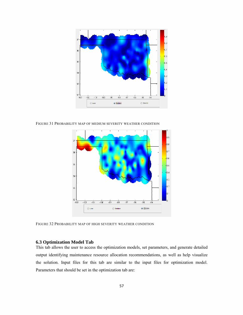
FIGURE 31 PROBABILITY MAP OF MEDIUM SEVERITY WEATHER CONDITION

FIGURE 32 PROBABILITY MAP OF HIGH SEVERITY WEATHER CONDITION

6.3 Optimization Model Tab This tab allows the user to access the optimization models, set parameters, and generate detailed

output identifying maintenance resource allocation recommendations, as well as help visualize

the solution. Input files for this tab are similar to the input files for optimization model.

Parameters that should be set in the optimization tab are:

57

• 𝛽𝛽 value that can vary from 0 to 1.

• Maximum budget.

• Maximum time the model is allowed to run can be set as a parameter.

The check box in front of the maximum budget parameter will allow us to remove the budget

constraint from our model. The maximum time limit provided can result in suboptimal solutions,

but given the intractability of such large-scale stochastic optimization models, this is necessary

for the graceful termination of the optimization algorithm. A screenshot of the optimization

model tab is shown in Figure 33 and Figure 34 depicts the assignment of different treatments on

to the links.

FIGURE 33 OPTIMIZATION TAB SCREENSHOT

58

FIGURE 34 ILLUSTRATION OF LINK TREATMENTS FOUND BY THE OPTIMIZATION MODEL

6.4 Concluding Comments Ice storms accompanied by excessive winter precipitation are high-impact weather events for the

State of Oklahoma. Such hazardous conditions dramatically reduce road transportation

infrastructure serviceability, and decrease safety. Consequently, these high-impact weather events

are a planning and preparedness priority for ODOT. This OkTC project combines weather

prediction models, risk-analysis, and optimization techniques to develop a prototype decision

support system that recommends optimal resource allocation and risk mitigation strategies under

severe winter weather emergencies.

The prediction of severe winter weather in the form of regional and temporal distribution of

ice/snow thickness is based on artificial neural network and particle filtering approaches that

include forecasts from SREF model as inputs. An appropriate loss function was developed which

depends on the distribution of ice/snow thickness, and the reduction in traffic flow due to reduced

system capacity. A stochastic optimization mode is developed that allocates winter maintenance

resources to minimize the conditional value-at-risk of losses, which leads to risk-averse resource

allocation recommendations.

The mathematical models developed to quantify storm severity, predict transportation specific

weather conditions, and to optimally allocate maintenance resources have been implemented in a

prototype decision support system and tested on a combination of real and synthetic data. The

deliverable developed and its individual modules show the potential for sophisticated models in

59

better aiding transportation decision-making. They also helped us identify several basic research

challenges in modeling and methodology that need to be addressed to expand the scalability and

resolution of the approaches developed in this project. This project has laid the foundation for

future studies along these lines, and has produced a useful and comprehensive deliverable

developed over its two year duration.

60

7. References [1] National Weather Service. "Online Glossary," www.weather.gov/glossary, Accessed 2011.

[2] Federal Emergency Management Agency. "Disaster Search," www.fema.gov/femaNews/disasterSearch.do?action=Reset, 2011.

[3] S. A. Changnon, “Catastrophic Winter Storms: An Escalating Problem,” Climate Change, vol. 84, pp. 131-139, 2007.

[4] S. A. Changnon, D. Changnon and T. R. Karl, “Temporal And Spatial Characteristics Of Snowstorms In The Contiguous United States,” Journal of Applied Meteorology and Climatology, vol. 45, pp. 1141-1155, 2006.

[5] S. A. Changnon, “Frequency Distributions Of Heavy Snowfall From Snowstorms In The United States,” Journal of Hydrologic Engineering, vol. 11, pp. 427, 2006.

[6] M. L. Branick, “Monthly And Geographic Distribution Of Heavy Snow Events In Oklahoma: 1951-2001,” National Weather Service, Technical Attachment, 2002.

[7] K. Jones, R. Thorkildson and N. Lott, “The Development Of A U.S. Climatology Of Extreme Ice Loads,” National Climatic Data Center: Technical Report, 2002.

[8] S. A. Changnon and T. R. Karl, “Temporal And Spatial Variations Of Freezing Rain In The Contiguous United States: 1948-2000,” Journal Of Applied Meteorology And Climatology, vol. 42, pp. 1302-1315, 2003.

[9] S. A. Changnon, “Characteristics Of Ice Storms In The United States,” Journal of applied meteorology and climatology, vol. 42, pp. 630-639, 2003.

[10] R. M. Rauber, L. S. Olthoff, M. K. Ramamurthy, D. Miller and K. E. Kunkel , “A Synoptic Weather Pattern And Sounding-Based Climatology Of Freezing Precipitation In The United States East Of The Rocky Mountains,” Journal Of Applied Meteorology And Climatology, vol. 40, pp. 1724-1747, 2001.

[11] D. A. Call, “Changes In Ice Storm Impacts Over Time: 1886-2000.,” Weather, Climate, and Society, vol. 2, pp. 23-35, 2010.

[12] Federal Emergency Management Agency."Presidential Disaster Declaration: 10 January 2000 - 1 January 2010," www.gismaps.fema.gov/recent.pdf, 2011.

[13] Federal Emergency Management Agency. "Presidential Disaster Declarations: 24 December 1964 - 1 January 2010," www.gismaps.fema.gov/historical.pdf, 2011.

[14] National Oceanic and Atmospheric Administration. "Storm Data Reference Note," www.ncdc.noaa.gov/oa/climate/sd/referencenotes.pdf, Accessed 2011.

[15] P. R. Orszag. "Memorandum For The Heads Of Executive Departments And Agencies: Open Government Directive," www.whitehouse.gov/open/documents/open-government-directive, Accessed 2011

[16] Federal Emergency Management Agency. “Public Assistance Funded Projects Summary,” www.data.gov, 2011.

[17] Federal Emergency Management Agency." Disaster Declaration Summary," www.data.gov, 2011.

61

http://www.weather.gov/glossary

http://www.fema.gov/femaNews/disasterSearch.do?action=Reset

http://www.gismaps.fema.gov/recent.pdf

http://www.gismaps.fema.gov/historical.pdf

http://www.ncdc.noaa.gov/oa/climate/sd/referencenotes.pdf

http://www.whitehouse.gov/open/documents/open-government-directive

http://www.data.gov/


[18] Federal Emergency Management Agency. "Hazard Mitigation Program Summary," www.data.gov, 2011.

[19] Federal Emergency Management Agency. "The Disaster Process and Disaster Aid Programs," www.fema.gov/hazard/dproc.shtm, 2011.

[20] National Weather Service. "Online Glossary," www.weather.gov/glossary, Accessed 2011.

[21] M. L. Branick, “A Climatology Of Significant Winter-Type Weather Events In The Contiguous United States,” Weather and Forecasting, vol. 12, pp. 193-207, 1997.

[22] Oklahoma Wind Power Initiative."Oklahoma Wind Resource Map: Estimated Wind Speeds at 50 Meters," www.ocgi.okstate.edu/owpi/OKWindInfo/OWPI_documents/OK_Wind_Resource_Map.pdf,

[23] R. M. Schwartz and T. W. Schmidlin, “Climatology Of Blizzards In The Conterminous United States: 1959-2000,” Journal of Climate, vol. 15, pp. 1765-1772, 2002.

[24] D. A. Call, “Changes In Ice Storm Impacts Over Time: 1886-2000,” Weather, Climate, and Society, vol. 2, pp. 23-35, 2010.

[25] S. A. Changnon, “Trend Analysis: Are Storms Getting Worse?,” Weatherwise, vol. 63, pp. 38-43, 2010.

[26] Federal Highway Administration."Priority, Market-Ready Technologies and Innovations," 2006, http://www.fhwa.dot.gov/resourcecenter/teams/operations/ops_mrt1.pdf

[27] Federal Highway Administration."Road Weather Management," 2004, http://ops.fhwa.dot.gov/aboutus/one_pagers/rwm.htm

[28] Colorado Department of Transportation, "Winter Maintenance," www.coloradodot.info/travel/winter-driving/faqs.html, 2011.

[29] Indiana Department of Transportation, "Winter Driving Safety," www.in.gov/indot/2795.htm, 2011.

[30] Virginia Department of Transportation, "VDOT prepares for winter," www.virginiadot.org/newsroom/snowseason.asp, 2011.

[31] Washington State Department of Transportation, "Snow and Ice Plan," www.wsdot.wa.gov/winter/SnowIcePlan.htm, 2011.

[32] "State Emergency Operations Plan (EOP)," Oklahoma Department of Emergency Management, 2009. http://www.ok.gov/OEM/Programs_&_Services/Planning/State_Emergency_Operations_Plan_-_EOP.html

[33] Department of Transportation, "New Ideas For A Nation On The Move," www.dot.gov/stratplan2011/dotstrategicplan.pdf, 2011.

[34] T. H. Maze, C. Albrecht, D. Kroeger and J. Wiegand, “Performance Measures For Snow And Ice Control Operations,” National Cooperative Highway Research Program Research Result Digest, vol. 335, 2009.

[35] M. Hulme, “A new winter index and geographical variations in winter weather,” Journal of Meteorology, vol. 7, pp. 294-300, 1982.

62


http://www.fema.gov/hazard/dproc.shtm

http://www.weather.gov/glossary

http://www.ocgi.okstate.edu/owpi/OKWindInfo/OWPI_documents/OK_Wind_Resource_Map.pdf

http://www.fhwa.dot.gov/resourcecenter/teams/operations/ops_mrt1.pdf

http://www.coloradodot.info/travel/winter-driving/faqs.html

http://www.coloradodot.info/travel/winter-driving/faqs.html

http://www.in.gov/indot/2795.htm

http://www.virginiadot.org/newsroom/snowseason.asp

http://www.wsdot.wa.gov/winter/SnowIcePlan.htm

http://www.dot.gov/stratplan2011/dotstrategicplan.pdf

[36] S. E. Boselly III, J. E. Thornes, C. Ulberg, "Road Weather Information Systems Volume 1, Research Report." Strategic Highway Research Program Publication - SHRP-H-350, National Research Council, Washington D.C., 1993. www4.trb.org/trb/onlinepubs.nsf/web/Highway_Operations_Reports

[37] M. C. Rissel and D. G. Scott, “Staffing Of Maintenance Crews During Winter Months,” Transportation Research Record, vol. 1019, pp. 12-21, 1985.

[38] J. Audrey, J. Li and B. Mills, "A Winter Index For Benchmarking Winter Road Maintenance Operations On Ontario Highways," Proceedings of the 2001 Annual Meeting of the Transportation Research Board, Transportation Research Board, 2001.

[39] C. G. Carmichael, W. A. G. Jr., B. R. Temeyer and M. K. Bryden , “A Winter Weather Index For Estimating Winter Roadway Maintenance Costs In The Midwest,” Journal of Applied Meteorology, vol. 43, no. 11, pp. 1783-1790, 2004.

[40] B. McCullouch, D. Belter, T. Konieczny and T. McClellan, "Indiana Winter Severity Index," Paper presented at the Sixth International Symposium on Snow Removal and Ice Control Technology, Transportation Research Board, 2004.

[41] W. A. Nixon and L. Qiu, "Developing A Storm Severity Index," Paper presented at the 2004 Annual Meeting of the Transportation Research Board, Transportation Research Board, 2004.

[42] G. Zielinski, “A Classification Scheme For Winter Storms In The Eastern And Central United States With An Emphasis On Nor'easters,” Bulletin of the American Meteorological Society, vol. 83, no. 1, pp. 37-51, 2001.

[43] G. McManus, S. F. Piltz, S. Sperry, R. A. McPherson, A. D. Gartside, D. McClain, T. Meyer, C. Fetsch and M. A. Shafer, "Development And Testing Of An Ice Accumulation Algorithm," 17th AMS Conference on Applied Climatology, American Meteorological Society, 2008.

[44] Developmental Testbed Center. "About The Weather Research And Forecasting Model," www.wrf-model.org/index.php, 2011.

[45] National Oceanic and Atmospheric Administration. "Short-Range Ensemble Forecasting," www.emc.ncep.noaa.gov/mmb/SREF/SREF.html, 2011.

[46] M. Kyte, Z. Khatib, P. Shannon and F. Kitchener, "Effect Of Environmental Factors On Free-Flow Speed." Transportation Research Circular E-C018: 4th International Symposium on Highway Capacity, pp. 108-119.

[47] K. F. Jones, “A Simple Model For Freezing Rain Ice Loads,” Atmospheric research, vol. 46, no. 1-2, pp. 87-97, 1998.

[48] National Climate Data Center. "Estimating The Water Equivalent Of Snow," www.ncdc.noaa.gov/oa/climate/conversion/newsnowfall.pdf, 2011.

[49] J. Jackson. "All About Mixed Winter Precipitation,” www.erh.noaa.gov/rnk/Newsletter/Fall_2008/mixed_precip/Mixed_precip.html, 2011.

[50] R. Rasmussen and J. A. Cole.National Center for Atmospheric Research, "How Snow Can Fool Pilots," www.rap.ucar.edu/projects/wsddm/SNOFOOL.pdf, 2011.

63

http://www.wrf-model.org/index.php

http://www.wrf-model.org/index.php

http://www.emc.ncep.noaa.gov/mmb/SREF/SREF.html

http://www.ncdc.noaa.gov/oa/climate/conversion/newsnowfall.pdf

http://www.erh.noaa.gov/rnk/Newsletter/Fall_2008/mixed_precip/Mixed_precip.html

http://www.rap.ucar.edu/projects/wsddm/SNOFOOL.pdf

[51] H. Rakha, M. Farzaneh, M. Arafeh and E. Sterzin, “Inclement Weather Impacts On Freeway Traffic Stream Behavior,” Transportation Research Record: Journal of the Transportation Research Board, vol. 2071, no. -1, pp. 8-18, 2008.

[52] Oklahoma Highway Safety Office. “Crash Data and Statistics." http://ok.gov/ohso/Data/Crash_Data_and_Statistics/index.html, Accessed 2011.

[53] American Meteorological Society. "Enhancing Weather Information With Probability Forecasts," Bulletin of the American Meteorological Society, pp. 450–452: 2002.

[54] T. N. Palmer, “Predicting Uncertainty In Forecasts Of Weather And Climate,” Reports on Progress in Physics, vol. 63, no. 2, pp. 71, 2000.

[55] M. Roulston, G. Bolton, A. Kleit and A. L. Sears-Collins, “A Laboratory Study Of The Benefits Of Including Uncertainty Information In Weather Forecasts,” Weather and Forecasting, vol. 21, no. 1, pp. 116-122, 2006.

[56] J. Torres, A. Garcia, M. De Blas and A. De Francisco, “Forecast Of Hourly Average Wind Speed With ARMA Models In Navarre (Spain),” Solar Energy, vol. 79, no. 1, pp. 65-77, 2005.

[57] P. Burlando, R. Rosso, L. Cadavid and J. D. Salas, “Forecasting Of Short-Term Rainfall Using ARMA Models,” Journal of Hydrology, vol. 144, no. 1-4, pp. 193-211, 1993.

[58] Z. Huang and Z. Chalabi, “Use Of Time-Series Analysis To Model And Forecast Wind Speed,” Journal of Wind Engineering and Industrial Aerodynamics, vol. 56, no. 2-3, pp. 311-322, 1995.

[59] A. Harvey, Forecasting, Structural Time Series Models And The Kalman Filter: Cambridge: University Press, 1989.

[60] P. Houtekamer, H. Mitchell, G. Pellerin, M. Buehner, M. Charron, L. Spacek and B. Hansen, “Atmospheric Data Assimilation With An Ensemble Kalman Filter: Results With Real Observations,” Monthly Weather Review, vol. 133, no. 3, pp. 604-620, 2005.

[61] G. Evensen, “The Ensemble Kalman Filter: Theoretical Formulation And Practical Implementation,” Ocean dynamics, vol. 53, no. 4, pp. 343-367, 2003.

[62] E. Ott, B. Hunt, I. Szunyogh, A. V. Zimin, E. J. Kostelich, M. Corazza, E. Kalnay, D. J. Patil, J. A. Yorke, “A Local Ensemble Kalman Filter For Atmospheric Data Assimilation,” Tellus A, vol. 56, no. 5, pp. 415-428, 2004.

[63] K. Ide and M. Ghil, “Extended Kalman Filtering For Vortex Systems. Part 1: Methodology And Point Vortices,” Dynamics of Atmospheres and Oceans, vol. 27, no. 1-4, pp. 301-332, 1998.

[64] A. Sfetsos, “A Comparison Of Various Forecasting Techniques Applied To Mean Hourly Wind Speed Time Series,” Renewable Energy, vol. 21, no. 1, pp. 23-35, 2000.

[65] W. Hsieh and B. Tang, “Applying Neural Network Models To Prediction And Data Analysis In Meteorology And Oceanography,” Bulletin of the American Meteorological Society, vol. 79, no. 9, pp. 1855-1870, 1998.

[66] M. Gardner and S. Dorling, “Artificial Neural Networks (The Multilayer Perceptron)—A Review Of Applications In The Atmospheric Sciences,” Atmospheric Environment, vol. 32, no. 14-15, pp. 2627-2636, 1998.

64

[67] V. Zavala, E. Constantinescu, T. Krause and M. Anitescu, “On-line economic Optimization Of Energy Systems Using Weather Forecast Information,” Journal of Process Control, vol. 19, no. 10, pp. 1725-1736, 2009.

[68] D. Cornford, “Flexible Gaussian process wind field models,” 1998.

[69] P. J. Roebber, M. R. Butt, S. J. Reinke and T. J. Grafenauer, “Real-time Forecasting Of Snowfall Using A Neural Network,” Weather and Forecasting, vol. 22, no. 3, pp. 676-684, 2007.

[70] P. J. Roebber, S. L. Bruening, D. M. Schultz and J. V. Cortinas Jr, “Improving Snowfall Forecasting By Diagnosing Snow Density,” Weather and Forecasting, vol. 18, no. 2, pp. 264-287, 2003.

[71] D. L. McGinnis, “Predicting Snowfall From Synoptic Circulation: A Comparison Of Linear Regression And Neural Network Methodologies,” Neural Nets: Applications in Geography, pp. 79–94, 1994.

[72] Mesonet. http://www.mesonet.org/, Accessed 2011.

[73] L. D. Minsk, Snow and Ice Control Manual for Transportation Facilities: NewYork: McGraw-Hill, 1998.

[74] R. T. Rockafellar and S. Uryasev, “Optimization Of Conditional Value-At-Risk,” The Journal of Risk, vol. 2, no. 3, pp. 21-41, 2000.

[75] R. T. Rockafellar and S. Uryasev., “Conditional Value-At-Risk For General Loss Distribution,” Journal of banking & finance, vol. 26, no. 7, pp. 1443-1471, 2002.

65

http://www.mesonet.org/

31, 2012 . 6. PERFORMING ORGANIZATION CODE 7. AUTHOR(S) Balabhaskar Balasundaram . Satish T.S....

Documents

Transcript of 31, 2012 . 6. PERFORMING ORGANIZATION CODE 7. AUTHOR(S) Balabhaskar Balasundaram . Satish T.S....