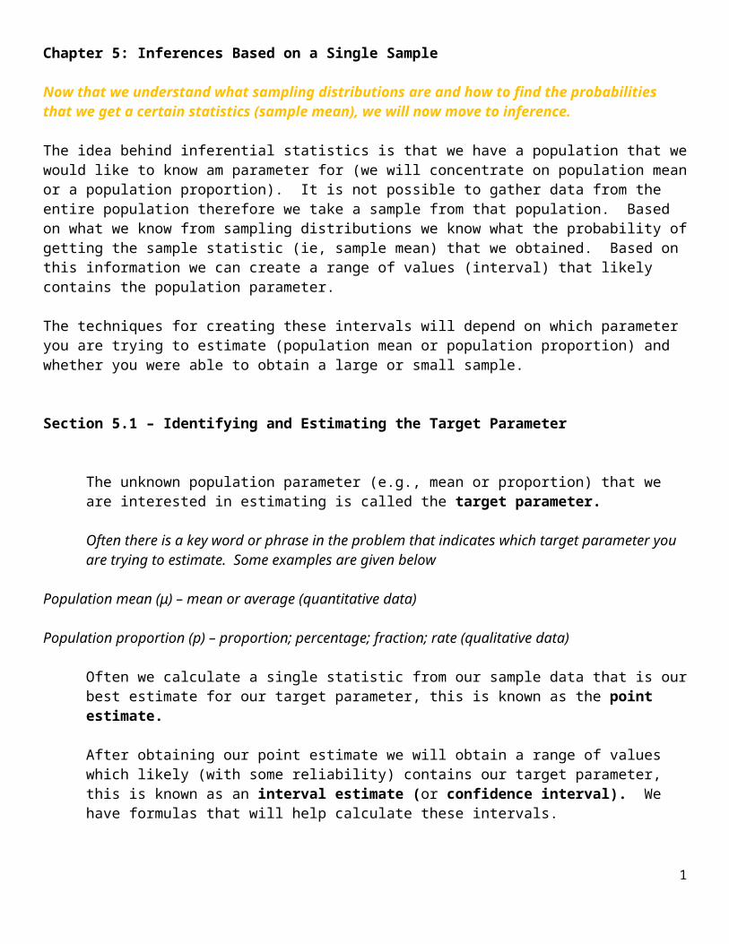
Chapter 5: Inferences Based on a Single Sample

Now that we understand what sampling distributions are and how to find the probabilities that we get a certain statistics (sample mean), we will now move to inference.

The idea behind inferential statistics is that we have a population that we would like to know am parameter for (we will concentrate on population mean or a population proportion). It is not possible to gather data from the entire population therefore we take a sample from that population. Based on what we know from sampling distributions we know what the probability of getting the sample statistic (ie, sample mean) that we obtained. Based on this information we can create a range of values (interval) that likely contains the population parameter.

The techniques for creating these intervals will depend on which parameter you are trying to estimate (population mean or population proportion) and whether you were able to obtain a large or small sample.

Section 5.1 – Identifying and Estimating the Target Parameter

The unknown population parameter (e.g., mean or proportion) that we are interested in estimating is called the target parameter.

Often there is a key word or phrase in the problem that indicates which target parameter you are trying to estimate. Some examples are given below

Population mean (μ) – mean or average (quantitative data)

Population proportion (p) – proportion; percentage; fraction; rate (qualitative data)

Often we calculate a single statistic from our sample data that is our best estimate for our target parameter, this is known as the point estimate.

After obtaining our point estimate we will obtain a range of values which likely (with some reliability) contains our target parameter, this is known as an interval estimate (or confidence interval). We have formulas that will help calculate these intervals.

Section 5.2 – Confidence Interval for a Population Mean: Normal (z) statistic

The general formula for a confidence interval is:Point estimate ± (critical value) (st. deviation of point estimate)

Recall that for large samples the sampling distribution for a sample mean is normally distributed with mean μ x̄=E ( x̄ )=μ and standard deviation

1

. When creating our interval estimate we have to have a measure of reliability (how sure are we that our interval contains the population parameter), this is known as the confidence coefficient.

The confidence coefficient is the probability that a randomly selected confidence interval encloses the population parameter – that is, the relative frequency with which similarly constructed intervals enclose the population parameter when the estimator is used repeatedly a very large number of times. The confidence level is the confidence coefficient expressed as a percentage.

For large samples our confidence interval for μ is:

x̄±(zα2)(σ√n )

- x̄ is the point estimate for the population parameter μ

- (zα 2) is our confidence coefficient – it is a z-score (number of st. deviations away from mean)

with the area to the right is α2 and (1−α ) is the confidence coefficient

2

There are some commonly used values for (zα2)

- ( σ√n ) is the standard deviation of the point estimate

In order for this confidence interval to be valid there are certain conditions that must be met…

Conditions Required for a Valid Large-Sample Confidence Interval for μ1. A random sample is selected from the target population.2. The sample size n is large (n ≥ 30). Due to the Central Limit Theorem, this condition guarantees that

the sampling distribution of x̄ is approximately normal. Also, for large n, s will be a good estimator of σ.)

Example - In a sample of 100 randomly selected employees, it was found that their mean height was 63.4 inches. From previous studies, it is assumed that the standard deviation, σ, is 2.4. Compute the 95% confidence interval for μ.

3

Example - A group of 49 randomly selected parrots has a mean age of 22.4 years with a population standard deviation of 3.8. Compute the 98% confidence interval for μ.

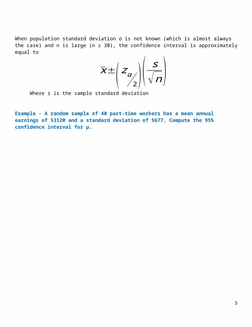
When population standard deviation σ is not known (which is almost always the case) and n is large (n ≥ 30), the confidence interval is approximately equal to

x̄±(zα2)(s

√n )Where s is the sample standard deviation

Example - A random sample of 40 part-time workers has a mean annual earnings of $3120 and a standard deviation of $677. Compute the 95% confidence interval for μ.

4

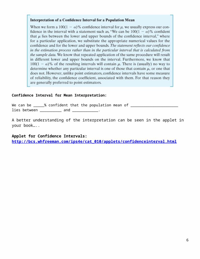
Confidence Interval for Mean Interpretation:

We can be _____% confident that the population mean of ______________________ lies between __________ and ____________.

A better understanding of the interpretation can be seen in the applet in your book…..

Applet for Confidence Intervals:http://bcs.whfreeman.com/ips4e/cat_010/applets/confidenceinterval.html

5

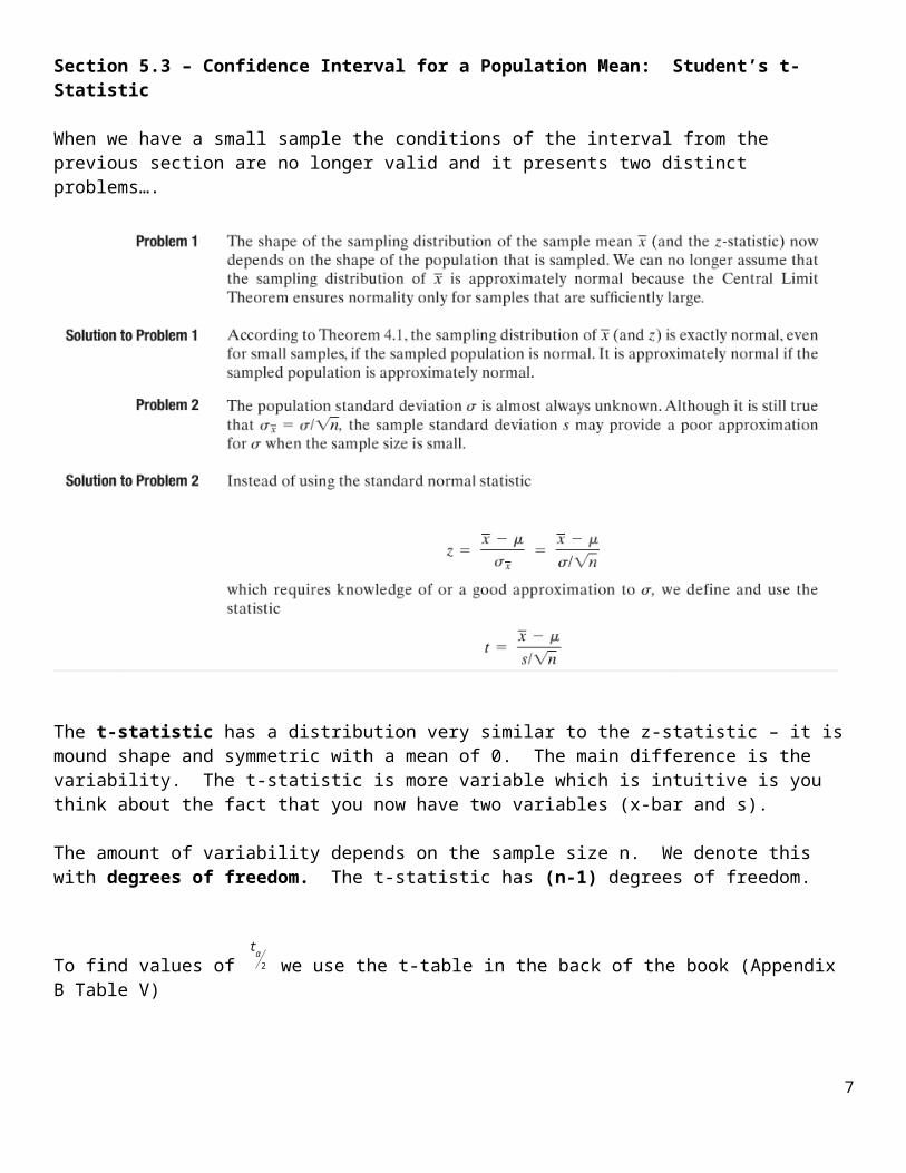
Section 5.3 – Confidence Interval for a Population Mean: Student’s t-Statistic

When we have a small sample the conditions of the interval from the previous section are no longer valid and it presents two distinct problems….

The t-statistic has a distribution very similar to the z-statistic – it is mound shape and symmetric with a mean of 0. The main difference is the variability. The t-statistic is more variable which is intuitive is you think about the fact that you now have two variables (x-bar and s).

The amount of variability depends on the sample size n. We denote this with degrees of freedom. The t-statistic has (n-1) degrees of freedom.

To find values of tα2 we use the t-table in the back of the book (Appendix B Table V)

6

Small Sample Confidence Interval for μ

x̄±(tα 2)(s

√n )Where t is based on (n-1) degrees of freedomConditions Required for a Valid Small-Sample Confidence Interval for μ

1. A random sample is selected from the target population2. The population has a relative frequency distribution that is approximately normal.

Example - Construct a 99% confidence interval for the population mean, μ. Assume the population has a normal distribution. A group of 19 randomly selected employees has a mean age of 22.4 years with a standard deviation of 3.8 years.

Example - Construct a 90% confidence interval for the population mean, μ. Assume the population has a normal distribution. A sample of 15 randomly selected math majors has a grade point average of 2.86 with a standard deviation of 0.78.

7

Section 5.4 – Large-Sample Confidence Interval for a Population Proportion

We now want to estimate the population proportion (the Binomial probability of success) rather than the population mean. This is the situation where you have qualitative data and want to estimate what percentage or proportion of the population has a particular quality of interest (this is particularly useful for polling data with election).

In order to create an interval estimate for the population proportion we need to know the sampling distribution of the sample proportion ( p̂ ).

Sampling Distribution of p̂1. The mean of the sampling distribution of p̂ is p; that is p̂ is an unbiased estimator of p.

2. The standard deviation of the sampling distribution of p̂ is √ pqn ; that is

3. For large samples, the sampling distribution of p̂ is approximately normal. A sample size is considered

large if both n p̂≥15 and n q̂≥15 .

Therefore, our confidence interval with for population proportion (p) from large samples is…

Large Sample Confidence Interval for p

p̂±(zα 2)(√ pqn )≈ p̂±( zα2)(√ p̂ q̂n )

Where p̂= xn and q̂=1− p̂

Conditions Required for a Valid Large-Sample Confidence Interval for p1. A random sample is selected from the target population.

2. The sample size n is large. (This condition will be satisfied if both n p̂≥15 and n q̂≥15 . Note that n p̂and n q̂ are simply the number of successes and number of failures, respectively, in the sample.

8

Example - A university dean is interested in determining the proportion of students who receive some sort of financial aid. Rather than examine the records for all students, the dean randomly selects 200 students and finds that 118 of them are receiving financial aid. Use a 95% confidence interval to estimate the true proportion of students on financial aid.

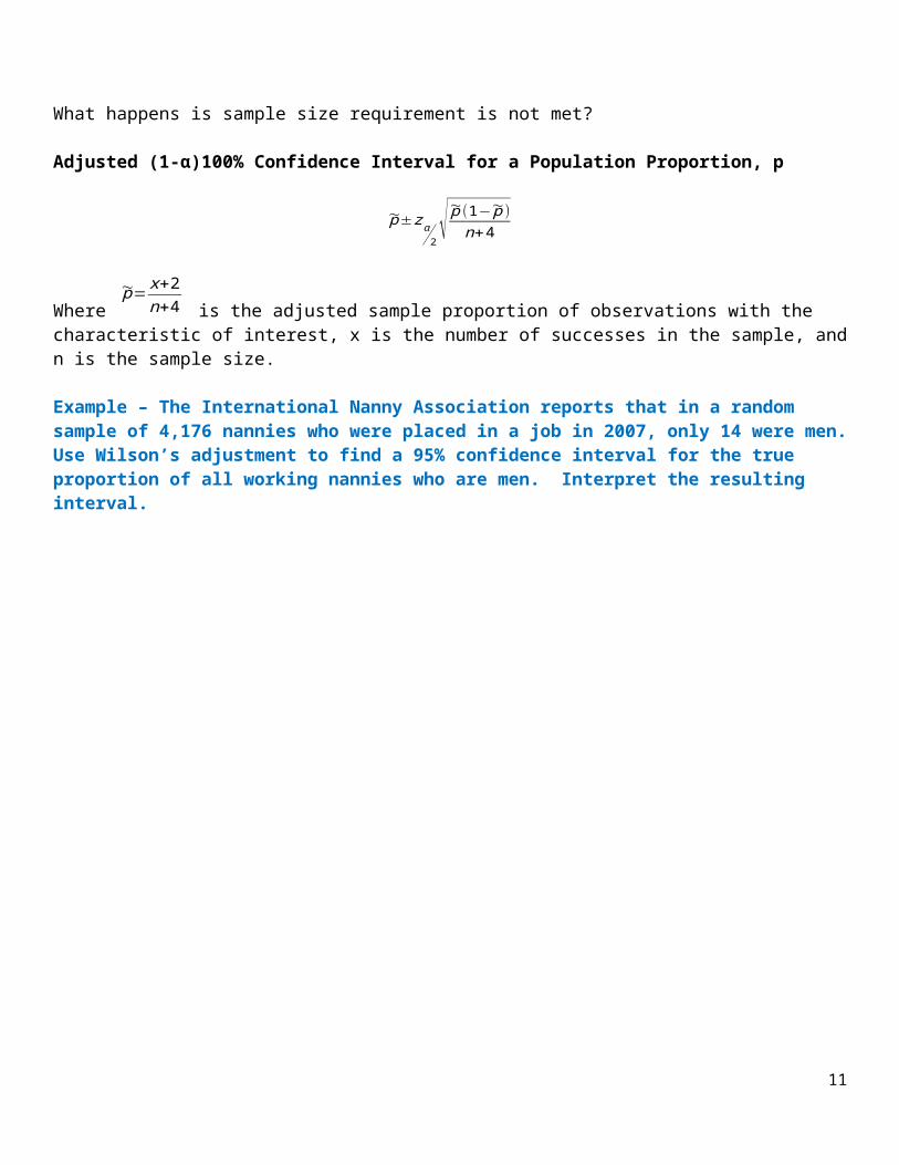
What happens is sample size requirement is not met?

Adjusted (1-α)100% Confidence Interval for a Population Proportion, p

~p±zα2√

~p (1−~p )n+4

Where ~p= x+2

n+4 is the adjusted sample proportion of observations with the characteristic of interest, x is the number of successes in the sample, and n is the sample size.

Example – The International Nanny Association reports that in a random sample of 4,176 nannies who were placed in a job in 2007, only 14 were men. Use Wilson’s adjustment to find a 95% confidence interval for the true proportion of all working nannies who are men. Interpret the resulting interval.

9

10

Section 5.5 – Determining the Sample Size

When estimating the Population Mean or Population Proportion it is sometimes helpful to know what sample size would be needed in order for you confidence interval to be within a certain amount at a given confidence level.

For a confidence interval to be “within” a certain amount what you add and subtract to the point estimate (critical value x st. deviation of point estimate) should be that amount. You are adding and subtracting this amount, this amount is called the sampling error or margin of error

Sample Size Determination for 100(1-α)% Confidence Interval for μ

In order to estimate μ with a sampling error and with 100(1-α)% confidence, the required sample size is found as follows:

zα2( σ√n )=SE

The solution for n is given by the equation

n=(zα2)

2 σ2

(SE )2

Note: The value of σ is usually unknown. It can be estimated by the standard deviation s, from a prior sample. Alternatively, we may approximate the rage R of observations in the population, and (conservatively) estimate σ ≈ R/4. In any case, you should round the value of n obtained upward to ensure that the sample size will be sufficient to achieve the specified reliability

Example - In order to set rates, an insurance company is trying to estimate the average number of sick days that full time workers at a local bank take per year. A previous study indicated that the standard deviation was 2.8 days. a) How large a sample must be selected if the company wants to be 90% confident that the true mean differs from the sample mean by no more than 1 day? b) Repeat part (a) using a 95% confidence interval. Which level of confidence requires a larger sample size? Explain.

11

Estimating Population Proportion

Sample Size Determination for 100(1-α)% Confidence Interval for pIn order to estimate the binomial probability p with sampling error SE and with 100(1-α)% confidence, the required sample size is found by solving the following equation for n:

The solution for n can be written as follows:

n=(zα2)

2 ( pq )

(SE )2

Note: Because the value of the product pq is unknown, it can be estimated by using the sample fraction of successes, p̂ , from a prior sample. Remember that the value of pq is at a maximum when p equals .5, so you can obtain conservatively large values of n by approximating p by .5 or values close to .5. In any case, you should round the value of n obtained upward to ensure that the sample size will be sufficient to achieve the specified reliability.

Example - In a college student poll, it is of interest to estimate the proportion p of students in favor of changing from a quarter-system to a semester-system. How many students should be polled so that we can estimate p to within 0.09 using a 99% confidence interval?

12