30408 two sph
17
AN ANALYTIC SOLUTION FOR LOW-FREQUENCY SCATTERING BY TWO SOFT SPHERES ∗ A. CHARALAMBOPOULOS †‡ , G. DASSI OS †‡ , AND M. HADJINICOLAOU †‡ SIAM J. APPL. MATH. c 1998 Society for Industrial and Appli ed Mathematics Vol. 58, No. 2, pp. 370–386, April 1998 002 Abstract. A plane wave is scatte red by two small spheres of not necessa rily equal radii. Low- frequency theory reduces this scattering problem to a sequence of potential problems which can be solved iteratively. It is shown that there exists exactly one bispherical coordinate system that fits the given geometry. Then R-separation is utilized to solve analytically the potential problems governing the leading two low-fr equ enc y approximations. It is sho wn that the Rayle igh approx imation is azimuthal indepen dent, while the first-o rder appro ximation involv es the azimuthal angle explicitly . The leading two nonv anishing approximations of the normalized scatteri ng amplitude as well as the scattering cross-section are also provided. The Rayleigh appro ximatio ns for the amplitude and for the cross-sec tion involv e only a monopole term, while their next order appro ximation s are expressed in terms of a monopol e as well as a dipole term. The dipol e term dis appe ars whenever the two spheres become equal, and this observation provides a way to determine whether the two spheres are equal or not, from far-field measu remen ts. Finall y , it is shown that for all practical purposes, first-order multiple scattering yields an excell ent approximation of this scattering process. Key words. bispherical coordinates, low-frequency scattering AMS subject classifications. 35C10, 35J25, 35P25 PII. S0036139996304081 1. Int roduction. The problem of direct and inverse scattering by a single ob- ject has been extensively investigated in the literature [2, 3]. F or some single shapes analytical results have been obtained for low frequency and high frequency as well as for any frequen cy [1, 4]. If the scat terin g region is compos ed of more than one con- nected component, then we refer to multiple scattering, since the wave field scattered by any one of the scatterers is received as an incident wave for the rest of the scatter- ers. For the mathematical formulation of multiple scattering problems we refer to the work of Twersk y [9, 10]. In [5] an analytic solution was obtained for scattering by a small sphere embedded in a half-space, based on an appropriate use of the bispherical coordinate system [6, 7, 8]. In the present work the bispherical system is further utilized to obtain the ana- lytic solution of the scattering problem corresponding to a plane wave that is incident upon two small spheres that are allow ed to have different radii. It is of interest to note that given the size and the position of the two spheres, there is exactly one bispherical coordinate system for which, as the spherical coordinate surface sweeps out the three-dimensional (3D) space, there are exactly two particular values of the correspondi ng coordinate va riab le that fit the giv en spheres. The two spheres are not allowed to touch each other. Hence, they describe a genuine two-body mul tipl e scatterin g probl em. The solutio n of the nonli near system that specifies the part icu- lar bispher ical syste m we seek is provided in the Appendix. The exterior boundary value problems that determine the leading two low-frequency approximations have been solv ed anal ytica lly. These closed form solut ions provid e results whic h, beside ∗ Received by the editors May 15, 1996; accepted for publicatio n (in revise d form) October 8, 1996. http://www.siam.org/journals/siap/58-2/30408.html † University of Patras, GR 265 00 Patras, Greece ([email protected]). ‡ Institute of Chemical Engineering and High Temperature Chemical Processes. 370
Transcript of 30408 two sph
7/31/2019 30408 two sph
http://slidepdf.com/reader/full/30408-two-sph 1/17
AN ANALYTIC SOLUTION FOR LOW-FREQUENCY SCATTERING
BY TWO SOFT SPHERES∗
A. CHARALAMBOPOULOS†‡ , G. DASSIOS†‡ , AND M. HADJINICOLAOU†‡
SIAM J. APPL. MATH. c 1998 Society for Industrial and Applied MathematicsVol. 58, No. 2, pp. 370–386, April 1998 002
Abstract. A plane wave is scattered by two small spheres of not necessarily equal radii. Low-frequency theory reduces this scattering problem to a sequence of potential problems which can besolved iteratively. It is shown that there exists exactly one bispherical coordinate system that fits thegiven geometry. Then R-separation is utilized to solve analytically the potential problems governingthe leading two low-frequency approximations. It is shown that the Rayleigh approximation isazimuthal independent, while the first-order approximation involves the azimuthal angle explicitly.The leading two nonvanishing approximations of the normalized scattering amplitude as well as thescattering cross-section are also provided. The Rayleigh approximations for the amplitude and forthe cross-section involve only a monopole term, while their next order approximations are expressedin terms of a monopole as well as a dipole term. The dipole term disappears whenever the twospheres become equal, and this observation provides a way to determine whether the two spheresare equal or not, from far-field measurements. Finally, it is shown that for all practical purposes,first-order multiple scattering yields an excellent approximation of this scattering process.
Key words. bispherical coordinates, low-frequency scattering
AMS subject classifications. 35C10, 35J25, 35P25
PII. S0036139996304081
1. Introduction. The problem of direct and inverse scattering by a single ob- ject has been extensively investigated in the literature [2, 3]. For some single shapesanalytical results have been obtained for low frequency and high frequency as well asfor any frequency [1, 4]. If the scattering region is composed of more than one con-nected component, then we refer to multiple scattering, since the wave field scatteredby any one of the scatterers is received as an incident wave for the rest of the scatter-ers. For the mathematical formulation of multiple scattering problems we refer to thework of Twersky [9, 10]. In [5] an analytic solution was obtained for scattering by a
small sphere embedded in a half-space, based on an appropriate use of the bisphericalcoordinate system [6, 7, 8].
In the present work the bispherical system is further utilized to obtain the ana-lytic solution of the scattering problem corresponding to a plane wave that is incidentupon two small spheres that are allowed to have different radii. It is of interest tonote that given the size and the position of the two spheres, there is exactly onebispherical coordinate system for which, as the spherical coordinate surface sweepsout the three-dimensional (3D) space, there are exactly two particular values of thecorresponding coordinate variable that fit the given spheres. The two spheres arenot allowed to touch each other. Hence, they describe a genuine two-body multiplescattering problem. The solution of the nonlinear system that specifies the particu-lar bispherical system we seek is provided in the Appendix. The exterior boundaryvalue problems that determine the leading two low-frequency approximations havebeen solved analytically. These closed form solutions provide results which, beside
∗Received by the editors May 15, 1996; accepted for publication (in revised form) October 8,1996.
http://www.siam.org/journals/siap/58-2/30408.html†University of Patras, GR 265 00 Patras, Greece ([email protected]).‡Institute of Chemical Engineering and High Temperature Chemical Processes.
370
7/31/2019 30408 two sph
http://slidepdf.com/reader/full/30408-two-sph 2/17
LOW-FREQUENCY SCATTERING BY TWO SOFT SPHERES 371
their significance to multiple scattering theory, can be used to check numerical codesdesigned to handle more general shapes.
Section 2 contains the statement of the scattering problem and its low-frequencytreatment. The zeroth-order, low-frequency approximation, known as Rayleigh ap-
proximation, is given in section 3, while in section 4 the solution of the first order of approximation is provided. The solution given in section 4 was possible through theuse of appropriate calculational techniques. Then orthogonality arguments lead to thecalculation of the surface integrals needed for the determination of both the scatteringamplitude and the scattering cross-section, in section 5. It is shown there that thefirst-order approximation for the scattering amplitude behaves as a monopole, whilethe second-order approximation involves a monopole term as well as a term that isproportional to the projection of the difference between the direction of incidence andthe direction of observation, on the axis connecting the centers of the two spheres.This term vanishes whenever the two spheres become equal. Hence, a dipole behaviorof the second-order low-frequency approximation in the far field establishes the factthat the two spheres have different radii. A similar situation holds true for the scat-tering cross-section, where the different sizes of the two spheres are coded in a dipole
term with respect to the direction of incidence, for the second-order approximationof the cross-section.
All the obtained results are given in terms of series which converge very rapidly.This series behavior reflects the multiple scattering characteristics of the two-bodysystem [9, 10]. A discussion of the results and some two-dimensional (2D) and 3Dgraphs showing the rapid convergence of the basic series involved are given in section6. From the graphs of the partial sums, it is easily shown that the first two terms of the series provide an approximation that is indistinguishable from the exact value of the infinite sum.
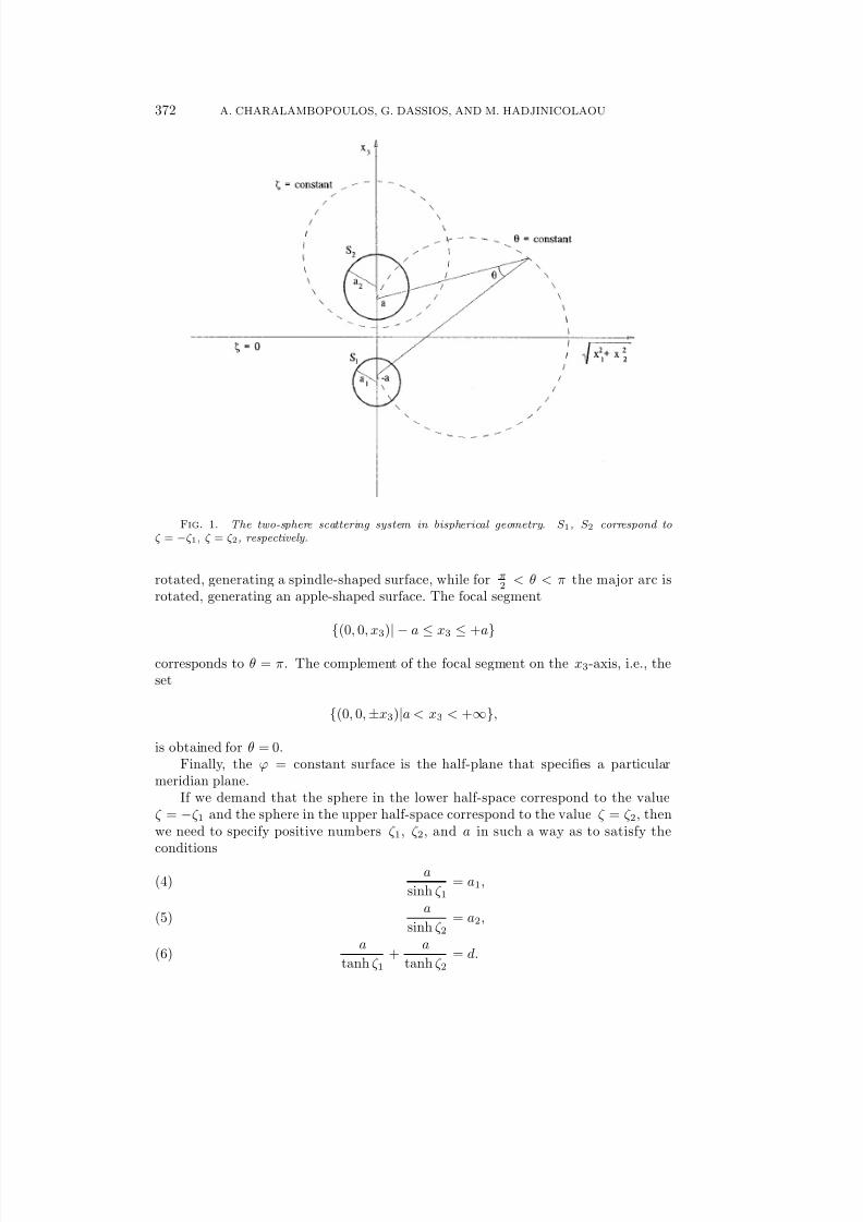
2. Statement of the problem. Let us consider two spheres of radii a1 and a2with centers that are located a distance d > a1 + a2 apart (Figure 1). Our first taskis to adapt a bispherical coordinate system in such a way as to be able to identify the
two given spheres with two specified values of one of the system variables.The bispherical system (ζ , θ, ϕ) is an orthogonal coordinate system [6, 7, 8] whichis connected to the cartesian system (x1, x2, x3) through the equations
x1 = asin θ cos ϕ
cosh ζ − cos θ,(1)
x2 = asin θ sin ϕ
cosh ζ − cos θ,(2)
x3 = asinh ζ
cosh ζ − cos θ,(3)
where 2a denotes the focii distance, ζ ∈ R specifies the nonintersecting spheres,θ ∈ [0, π] specifies the intersecting spheres, and ϕ ∈ [0, 2π) is the azimuthal anglewhich represents the axial symmetry of the bispherical system.
The coordinate surface ζ = constant is a sphere centered at the point(0, 0, a/tanh ζ ) with radius a/| sinh ζ |. As ζ runs from −∞ to +∞ the correspondingcoordinate sphere springs at the focus (0, 0, −a) for ζ → −∞, sweeps the x3 < 0half-space for ζ < 0, passes through the x3 = 0 plane for ζ = 0, and then sweeps thex3 > 0 half-space for ζ > 0 to end up at (0, 0, +a) for ζ → +∞.
The θ = constant surface is generated through rotation of a circular arc aroundits chord which coincides with the focal segment. For 0 < θ < π
2 the minor arc is
7/31/2019 30408 two sph
http://slidepdf.com/reader/full/30408-two-sph 3/17
372 A. CHARALAMBOPOULOS, G. DASSIOS, AND M. HADJINICOLAOU
FIG. 1. The two-sphere scattering system in bispherical geometry. S 1, S 2 correspond to
ζ = −ζ 1, ζ = ζ 2, respectively.
rotated, generating a spindle-shaped surface, while for π2 < θ < π the major arc is
rotated, generating an apple-shaped surface. The focal segment
{(0, 0, x3)
| −a
≤x3
≤+a
}corresponds to θ = π. The complement of the focal segment on the x3-axis, i.e., theset
{(0, 0, ±x3)|a < x3 < +∞},
is obtained for θ = 0.Finally, the ϕ = constant surface is the half-plane that specifies a particular
meridian plane.If we demand that the sphere in the lower half-space correspond to the value
ζ = −ζ 1 and the sphere in the upper half-space correspond to the value ζ = ζ 2, thenwe need to specify positive numbers ζ 1, ζ 2, and a in such a way as to satisfy theconditions
a
sinh ζ 1= a1,(4)
a
sinh ζ 2= a2,(5)
a
tanh ζ 1+
a
tanh ζ 2= d.(6)
7/31/2019 30408 two sph
http://slidepdf.com/reader/full/30408-two-sph 4/17
LOW-FREQUENCY SCATTERING BY TWO SOFT SPHERES 373
The nonlinear system (4)–(6) has the solution (see the appendix)
a =
d2 − (a1 − a2)2
d2 − (a1 + a2)2
2d,(7)
ζ 1 = ln d2 + (a1 − a2)(a1 + a2) +
d2 − (a1 − a2)2
d2 − (a1 + a2)2
2 da1,(8)
ζ 2 = lnd2 − (a1 − a2)(a1 + a2) +
d2 − (a1 − a2)2
d2 − (a1 + a2)2
2 da2,(9)
which, under the assumption that all ζ 1, ζ 2, and a are positive, is unique. There-fore, there is exactly one bispherical system that fits the given two-sphere scatteringobstacle, and this is shown in Figure 1.
The actual region where the scattered wave propagates is specified by the exteriorof the two spheres. This corresponds to the domain
V = {(ζ , θ , ϕ)|ζ ∈ (−ζ 1, ζ 2), θ ∈ [0, π], ϕ ∈ [0, 2π)}(10)
and forms a bispherical shell. The interior of the sphere S 1(ζ = −ζ 1) corresponds toζ ∈ (−∞, −ζ 1) and the interior of the sphere S 2(ζ = ζ 2) corresponds to ζ ∈ (ζ 2, +∞).
The spherical radial distance is given by
r = a
cosh ζ + cos θ
cosh ζ − cos θ,(11)
which implies that the far-field region corresponds to a small neighborhood of (ζ, θ) = (0, 0) in the bispherical domain.
Suppressing the harmonic time dependence exp{−iωt}, where ω denotes the an-gular frequency, and assuming the plane wave incidence
u
i
(r) = e
ik·r
,(12)
with k = kk̂ the propagation vector and k the wave number, we arrive at the followingscalar scattering problem for a pair of acoustically soft spheres.
Find the total field
u(r) = ui(r) + us(r), r ∈ V,(13)
which satisfies the Helmholtz equation
(∆ + k2)u(r) = 0, r ∈ V,(14)
and the boundary conditions
u(r) = 0, r ∈ S 1 ∪ S 2;(15)
the scattered field uS satisfies the Sommerfeld radiation condition
limr→∞
r
∂us
∂r− ikus
= 0(16)
uniformly over the unit sphere S 2.
7/31/2019 30408 two sph
http://slidepdf.com/reader/full/30408-two-sph 5/17
374 A. CHARALAMBOPOULOS, G. DASSIOS, AND M. HADJINICOLAOU
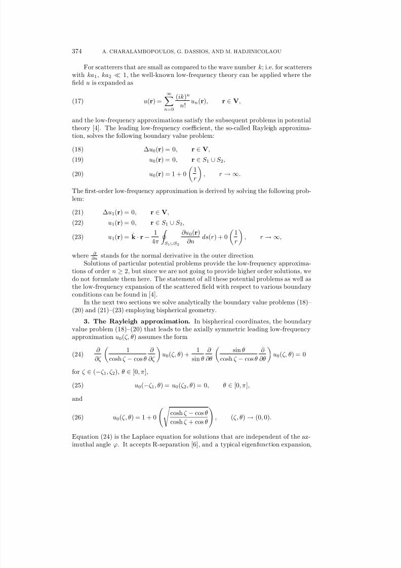
For scatterers that are small as compared to the wave number k; i.e. for scattererswith ka1, ka2 1, the well-known low-frequency theory can be applied where thefield u is expanded as
u(r) =
∞n=0
(ik)n
n! un(r), r ∈ V,(17)
and the low-frequency approximations satisfy the subsequent problems in potentialtheory [4]. The leading low-frequency coefficient, the so-called Rayleigh approxima-tion, solves the following boundary value problem:
∆u0(r) = 0, r ∈ V,(18)
u0(r) = 0, r ∈ S 1 ∪ S 2,(19)
u0(r) = 1 + 0
1
r
, r → ∞.(20)
The first-order low-frequency approximation is derived by solving the following prob-
lem:
∆u1(r) = 0, r ∈ V,(21)
u1(r) = 0, r ∈ S 1 ∪ S 2,(22)
u1(r) = k̂ · r − 1
4π
S1∪S2
∂u0(r)
∂nds(r) + 0
1
r
, r → ∞,(23)
where ∂ ∂n stands for the normal derivative in the outer direction.
Solutions of particular potential problems provide the low-frequency approxima-tions of order n ≥ 2, but since we are not going to provide higher order solutions, wedo not formulate them here. The statement of all these potential problems as well asthe low-frequency expansion of the scattered field with respect to various boundaryconditions can be found in [4].
In the next two sections we solve analytically the boundary value problems (18)–(20) and (21)–(23) employing bispherical geometry.
3. The Rayleigh approximation. In bispherical coordinates, the boundaryvalue problem (18)–(20) that leads to the axially symmetric leading low-frequencyapproximation u0(ζ, θ) assumes the form
∂
∂ζ
1
cosh ζ − cos θ
∂
∂ζ
u0(ζ, θ) +
1
sin θ
∂
∂θ
sin θ
cosh ζ − cos θ
∂
∂θ
u0(ζ, θ) = 0(24)
for ζ ∈ (−ζ 1, ζ 2), θ ∈ [0, π],
u0(−ζ 1, θ) = u0(ζ 2, θ) = 0, θ ∈ [0, π],(25)
and
u0(ζ, θ) = 1 + 0
cosh ζ − cos θ
cosh ζ + cos θ
, (ζ, θ) → (0, 0).(26)
Equation (24) is the Laplace equation for solutions that are independent of the az-imuthal angle ϕ. It accepts R-separation [6], and a typical eigenfunction expansion,

7/31/2019 30408 two sph
http://slidepdf.com/reader/full/30408-two-sph 6/17
LOW-FREQUENCY SCATTERING BY TWO SOFT SPHERES 375
regular on the axis, assumes the form
f (ζ, θ) =
cosh ζ − cos θ
∞
n=0[Ane(n+
1
2)ζ + Bne−(n+
1
2)ζ ]P n(cos θ),(27)
where P n are the Legendre polynomials. A key formula in our work is provided bythe uniformly convergent expansion
1√cosh ζ − cos θ
=√
2∞n=0
e−(n+1
2)|ζ|P n(cos θ)(28)
given in [8] (formula (10.3.70)). Note that the expansion (28) is independent of thesemifocal distance a. In view of (26), (27), and (28) we seek solutions in the form
u0(ζ, θ) =
cosh ζ − cos θ∞n=0
[√
2e−(n+1
2)|ζ|
+ Ane(n+1
2)ζ + Bne−(n+
1
2)ζ ]P n(cos θ),
(29)
where the coefficients An and Bn are related through the boundary conditions (25),implying
An + e(2n+1)ζ1Bn = −√
2,(30)
An + e−(2n+1)ζ2Bn = −√
2e−(2n+1)ζ2(31)
for n = 0, 1, 2, . . . .Solving the system (30), (31) we obtain
An = −√
2e(2n+1)ζ1 − 1
e(2n+1)(ζ1+ζ2) − 1,(32)
Bn =
−
√2
e(2n+1)ζ2 − 1
e(2n+1)(ζ1+ζ2)
− 1
(33)
for n = 0, 1, 2, . . . .Substituting (32) and (33) into (29) we arrive at the analytic expression for the
Rayleigh approximation
u0(ζ, θ) =
cosh ζ − cos θ
∞n=0
I n(ζ )P n(cos θ),(34)
where
I n(ζ ) =√
2
e−(n+
1
2)|ζ| − e(2n+1)ζ1 − 1
e(2n+1)(ζ1+ζ2) − 1e(n+
1
2)ζ
−e(2n+1)ζ2
−1
e(2n+1)(ζ1+ζ2) − 1 e
−(n+ 1
2)ζ
.
(35)
Obviously, expression (34) for u0 satisfies Laplace equation (24) and the boundaryconditions (25). If we define the function
Γ(ζ ) =∞n=0
e(2n+1)ζ − 1
e(2n+1)(ζ1+ζ2) − 1,(36)
7/31/2019 30408 two sph
http://slidepdf.com/reader/full/30408-two-sph 7/17
376 A. CHARALAMBOPOULOS, G. DASSIOS, AND M. HADJINICOLAOU
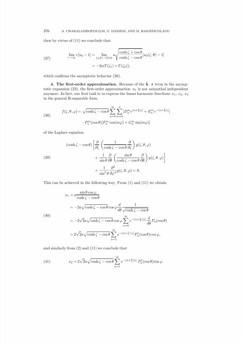
then by virtue of (11) we conclude that
limr→∞
r[u0 − 1] = lim(ζ,θ)→(0,0)
a cosh ζ + cos θ
cosh ζ −
cos θ[u0(ζ, θ) − 1]
= −2a(Γ(ζ 1) + Γ(ζ 2)),(37)
which confirms the asymptotic behavior (26).
4. The first-order approximation. Because of the k̂ · r term in the asymp-totic expansion (23), the first-order approximation u1 is not azimuthal independentanymore. In fact, our first task is to express the linear harmonic functions x1, x2, x3in the general R-separable form
f (ζ , θ , ϕ) =
cosh ζ − cos θ
∞
n=0n
m=0
[Dmn e(n+
1
2)ζ + E mn e−(n+
1
2)ζ]
· P mn (cos θ)[F mn cos(mϕ) + Gmn sin(mϕ)]
(38)
of the Laplace equation
(cosh ζ − cos θ)
∂
∂ζ
1
cosh ζ − cos θ
∂
∂ζ
g(ζ , θ , ϕ)
+1
sin θ
∂
∂θ
sin θ
cosh ζ − cos θ
∂
∂θ
g(ζ , θ , ϕ)
+1
sin2 θ
∂ 2
∂ϕ2g(ζ , θ , ϕ) = 0.
(39)
This can be achieved in the following way. From (1) and (11) we obtain
x1 = asin θ cos ϕ
cosh ζ − cos θ
= −2a
cosh ζ − cos θ cos ϕd
dθ
1√cosh ζ − cos θ
= −2√
2a
cosh ζ − cos θ cos ϕ∞n=0
e−(n+1
2)|ζ| d
dθP n(cos θ)
= 2√
2a cosh ζ − cos θ
∞
n=1
e−(n+1
2)|ζ|P 1n(cos θ)cos ϕ,
(40)
and similarly from (2) and (11) we conclude that
x2 = 2√
2a
cosh ζ − cos θ∞n=1
e−(n+1
2)|ζ|P 1n(cos θ)sin ϕ.(41)
7/31/2019 30408 two sph
http://slidepdf.com/reader/full/30408-two-sph 8/17
LOW-FREQUENCY SCATTERING BY TWO SOFT SPHERES 377
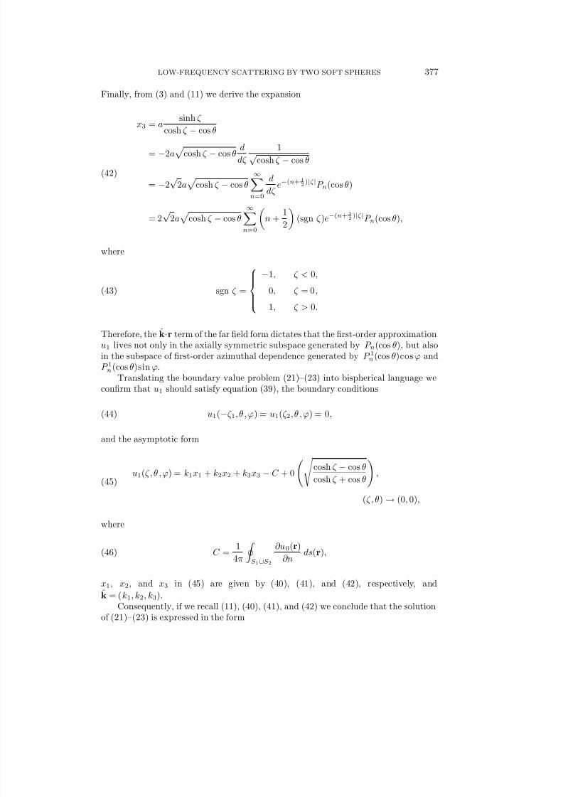
Finally, from (3) and (11) we derive the expansion
x3 = asinh ζ
cosh ζ
−cos θ
= −2a
cosh ζ − cos θd
dζ
1√cosh ζ − cos θ
= −2√
2a
cosh ζ − cos θ
∞n=0
d
dζ e−(n+
1
2)|ζ|P n(cos θ)
= 2√
2a
cosh ζ − cos θ∞n=0
n +
1
2
(sgn ζ )e−(n+
1
2)|ζ|P n(cos θ),
(42)
where
sgn ζ =
−1, ζ < 0,0, ζ = 0,
1, ζ > 0.
(43)
Therefore, the k̂·r term of the far field form dictates that the first-order approximationu1 lives not only in the axially symmetric subspace generated by P n(cos θ), but alsoin the subspace of first-order azimuthal dependence generated by P 1n(cos θ)cos ϕ andP 1n(cos θ)sin ϕ.
Translating the boundary value problem (21)–(23) into bispherical language weconfirm that u1 should satisfy equation (39), the boundary conditions
u1(−ζ 1, θ , ϕ) = u1(ζ 2, θ , ϕ) = 0,(44)
and the asymptotic form
u1(ζ , θ , ϕ) = k1x1 + k2x2 + k3x3 − C + 0
cosh ζ − cos θ
cosh ζ + cos θ
,
(ζ, θ) → (0, 0),
(45)
where
C =1
4π S1∪S2
∂u0(r)
∂nds(r),(46)
x1, x2, and x3 in (45) are given by (40), (41), and (42), respectively, and
k̂ = (k1, k2, k3).Consequently, if we recall (11), (40), (41), and (42) we conclude that the solution
of (21)–(23) is expressed in the form
7/31/2019 30408 two sph
http://slidepdf.com/reader/full/30408-two-sph 9/17
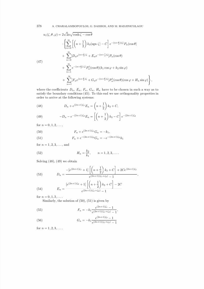
378 A. CHARALAMBOPOULOS, G. DASSIOS, AND M. HADJINICOLAOU
u1(ζ , θ , ϕ) = 2√
2a
cosh ζ − cos θ
·
∞
n=0
n +1
2
k3(sgn ζ ) − C
e−(n+
1
2)|ζ|P n(cos θ)
+∞n=0
[Dne(n+1
2)ζ + E ne−(n+
1
2)ζ ]P n(cos θ)
+∞n=1
e−(n+1
2)|ζ|P 1n(cos θ)(k1 cos ϕ + k2 sin ϕ)
+∞n=1
[F ne(n+1
2)ζ + Gne−(n+
1
2)ζ ]P 1n(cos θ)(cos ϕ + H n sin ϕ)
,
(47)
where the coefficients Dn, E n, F n, Gn, H n have to be chosen in such a way as tosatisfy the boundary conditions (45). To this end we use orthogonality properties inorder to arrive at the following systems:
Dn + e(2n+1)ζ1E n =
n +
1
2
k3 + C,(48)
−Dn − e−(2n+1)ζ2E n =
n +
1
2
k3 − C
e−(2n+1)ζ2(49)
for n = 0, 1, 2, . . . ,
F n + e(2n+1)ζ1Gn = −k1,(50)
F n + e−(2n+1)ζ2Gn = −e−(2n+1)ζ2k1(51)
for n = 1, 2, 3, . . . , and
H n = k2k1
, n = 1, 2, 3, . . . .(52)
Solving (48), (49) we obtain
Dn =
−[e(2n+1)ζ1 + 1]
n +
1
2
k3 + C
+ 2Ce(2n+1)ζ1
e(2n+1)(ζ1+ζ2) − 1,(53)
E n =
[e(2n+1)ζ2 + 1]
n +
1
2
k3 + C
− 2C
e(2n+1)(ζ1+ζ2) − 1(54)
for n = 0, 1, 2, . . . .Similarly, the solution of (50), (51) is given by
F n = −k1e(2n+1)ζ1 − 1
e(2n+1)(ζ1+ζ2) − 1,(55)
Gn = −k1e(2n+1)ζ2 − 1
e(2n+1)(ζ1+ζ2) − 1(56)
for n = 1, 2, 3, . . . .
7/31/2019 30408 two sph
http://slidepdf.com/reader/full/30408-two-sph 10/17
LOW-FREQUENCY SCATTERING BY TWO SOFT SPHERES 379
Substituting (52)–(56) into (47) we derive the following analytic form of the first-order approximation:
u1(ζ , θ , ϕ) = 2√
2a√
cosh ζ − cos θ
·
∞n=0
K n(ζ )P n(cos θ) +∞n=1
Λn(ζ )P 1n(cos θ)(k1 cos ϕ + k2 sin ϕ)
,(57)
where, for n = 0, 1, 2, . . .
K n(ζ ) =
n +
1
2
k3(sgn ζ ) − C
e−(n+
1
2)|ζ|
−
n +
1
2
k3 − C
[e(2n+1)ζ1 + 1] + 2C
e(2n+1)(ζ1+ζ2) − 1e(n+
1
2)ζ
+n +
1
2 k3 + C [e(2n+1)ζ2 + 1] − 2C
e(2n+1)(ζ1+ζ2) − 1 e−(n+ 1
2)ζ
,
(58)
and for n = 1, 2, 3, . . .
Λn(ζ ) = e−(n+1
2)|ζ| − e(2n+1)ζ1 − 1
e(2n+1)(ζ1+ζ2) − 1e(n+
1
2)ζ − e(2n+1)ζ2 − 1
e(2n+1)(ζ1+ζ2) − 1e−(n+
1
2)ζ .(59)
It can easily be shown that the boundary conditions (42) imply that
K n(−ζ 1) = K n(ζ 2) = 0, n = 0, 1, 2, . . . ,(60)
and
Λn(−ζ 1) = Λn(ζ 2) = 0, n = 1, 2, 3, . . . .(61)
We observe here that the expression (k1 cos ϕ + k2 sin ϕ) denotes the inner productof the horizontal projections, of the direction of propagation k̂ and the direction of observation r̂, on a plane perpendicular to the axis of symmetry. Therefore, wheneverthe horizontal directions of k̂ and r̂ are perpendicular, the second series in the right-hand side of the solution (57) vanishes, and the first-order approximation u1 does notinvolve the azimuthal angle explicitly.
5. The far field. The scattered field us accepts the integral representation
us(r) = − ik
4π
S1∪S2
h(k|r − r|) ∂
∂nu(r) ds(r), r ∈ V,(62)
where
h(x) = eixix
(63)
is the fundamental solution of the Helmholtz operator in three dimensions. From therepresentation (62) we obtain the following asymptotic form:
us(r) = g(r̂, k̂)h(kr) + 0
1
r2
, r → ∞,(64)
7/31/2019 30408 two sph
http://slidepdf.com/reader/full/30408-two-sph 11/17
380 A. CHARALAMBOPOULOS, G. DASSIOS, AND M. HADJINICOLAOU
where
g(r̂, k̂) = − ik
4π
S1∪S2
e−ikr̂·r ∂u(r)
∂nds(r)(65)
denotes the scattering amplitude which is normalized to the same dimensions as us.Comparing (62) and (64) we see that the only difference between the representationof the near field (62) and that of the far field (65) is observed in the kernel function,which in (62) represents a point source located at r ∈ S 1∪S 2, while in (65) representsa point source situated at the origin, modified by the phase factor of a plane wave.Hence, the scattering amplitude describes how the obstacle responds in the far fieldand in the direction r̂, when it is excited by a plane wave propagating in the directionk̂. In other words, the scattering amplitude provides a directional analysis of theinteraction between the incident field and the obstacle as it is established far awayfrom the region of interaction. It has been proved in inverse scattering theory [3] thatthe scattering amplitude, also known as far-field pattern, registers all the informationboth of physical as well as geometrical character, about the scattering obstacle.
Low-frequency analysis of the scattering amplitude [4] leads to the approximation
g(r̂, k̂) = − ik
4π
S1∪S2
∂u0(r)
∂nds(r)
+k2
4π
S1∪S2
∂u1(r)
∂n− (r̂ · r)
∂u0(r)
∂n
ds(r) + 0(k3).
(66)
In order to obtain an analytic expression for the low-frequency approximation of thescattering amplitude, the three integrals in (66) must be evaluated.
In view of the metric coefficients
gζ = gθ =gϕ
sin2 θ=
a2
(cosh ζ − cos θ)2(67)
we confirm the expression
∂
∂n= n̂ · =
cosh ζ − cos θ
a
∂
∂ζ (68)
for the normal derivative and
ds(r) =a2 sin θ
(cosh ζ − cos θ)2dθdϕ(69)
for the surface element on the ζ = constant surface.As the variable ζ increases, it describes a sphere expanding in the lower half-
space, where ζ is negative, and a contracting sphere in the upper half-space, where ζ is positive. Therefore, the sign of the normal derivative on S 2 has to be reversed inorder to secure normal differentiation in the outer direction.
Consequently, in view of (25), which implies that
I n(−ζ 1) = I n(ζ 2) = 0, n = 0, 1, 2, . . . ,(70)
we arrive at
∂u0(r)
∂n
ζ=−ζ1
=(cosh ζ 1 − cos θ)3/2
a
∞n=0
I n(−ζ 1)P n(cos θ)(71)
7/31/2019 30408 two sph
http://slidepdf.com/reader/full/30408-two-sph 12/17
LOW-FREQUENCY SCATTERING BY TWO SOFT SPHERES 381
and
∂u0(r)
∂n
ζ=ζ2
= − (cosh ζ 2 − cos θ)3/2
a
∞n=0
I n(ζ 2)P n(cos θ).(72)
Substituting (69), (70), and (71) in the first integral on the right-hand side of (66)and using orthogonality arguments for the Legendre polynomials as well as the basicformula (28) we obtain
S1∪S2
∂u0(r)
∂nds(r)
= a∞n=0
I n(−ζ 1)
S1
P n(cos θ)sin θ√cosh ζ 1 − cos θ
dθdϕ
− a∞n=0
I n(ζ 2)
S2
P n(cos θ)sin θ√cosh ζ 2 − cos θ
dθdϕ
= 2√2πa
∞n=0
∞κ=0
[I n(−ζ 1)e−(κ+1
2 )ζ1 − I n(ζ 2)e−(κ+1
2 )ζ2 ]
· π0
P n(cos θ)P κ(cos θ)sin θ dθ
= 2√
2πa∞n=0
2
(2n + 1)[I n(−ζ 1)e−(n+
1
2)ζ1 − I n(ζ 2)e−(n+
1
2)ζ2 ].
(73)
Long but straightforward calculations verify that
I n(−ζ 1)e−(n+1
2)ζ1 − I n(ζ 2)e−(n+
1
2)ζ2
=√
2(2n + 1)e(2n+1)ζ1 + e(2n+1)ζ2 − 2
e(2n+1)(ζ1+ζ2)
− 1
.(74)
Therefore, in view of (36) and (74), the surface integral in (73) yields S1∪S2
∂u0(r)
∂nds(r) = 8πa(Γ(ζ 1) + Γ(ζ 2)),(75)
which also implies that
C = 2a(Γ(ζ 1) + Γ(ζ 2)).(76)
As a byproduct of the above calculations we recover the capacity [4] of the two sphereswhich is equal to 2a(Γ(ζ 1) + Γ(ζ 2)) (see [7]).
In a similar way, using (28), (57), (61), and (62), it is shown that
S1∪S2
∂u1(r
)∂n
ds(r)
= 16πa2∞n=0
1
2n + 1[K n(−ζ 1)e−(n+
1
2)ζ1 − K n(ζ 2)e−(n+
1
2)ζ2 ],
(77)
where the vanishing of the contributions from the terms involving the functions Λn(ζ )is due to the orthogonality with respect to the azimuthal angle.
7/31/2019 30408 two sph
http://slidepdf.com/reader/full/30408-two-sph 13/17
382 A. CHARALAMBOPOULOS, G. DASSIOS, AND M. HADJINICOLAOU
Some more calculations lead to
K n(−ζ 1)e−(n+1
2)ζ1 − K n(ζ 2)e−(n+
1
2)ζ2
= 2k3
n +
1
22 e(2n+1)ζ1
−e(2n+1)ζ2
e(2n+1)(ζ1+ζ2) − 1
− 2C
n +
1
2
e(2n+1)ζ1 + e(2n+1)ζ2 − 2
e(2n+1)(ζ1+ζ2) − 1,
(78)
which by substitution into (77) yields S1∪S2
∂u1(r)
∂nds(r)
= 8πa2k3
∞n=0
(2n + 1)e(2n+1)ζ1 − e(2n+1)ζ2
e(2n+1)(ζ1+ζ2) − 1
− 16πa
2
(Γ(ζ 1) + Γ(ζ 2))
2
.
(79)
Because of the uniform convergence of the series in (36), which defines the functionΓ(ζ ), we can easily conclude that
∞n=0
(2n + 1)e(2n+1)ζ1 − e(2n+1)ζ2
e(2n+1)(ζ1+ζ2) − 1= Γ(ζ 1) − Γ(ζ 2),(80)
which implies that S1∪S2
∂u1(r)
∂nds(r) = 8πa2k3(Γ(ζ 1) − Γ(ζ 2)) − 16πa2(Γ(ζ 1) + Γ(ζ 2))2.(81)
Combining techniques similar to that used to obtain (75) and (81) we arrive at thevalue of the third integral in (66), which is
S1∪S2
(r̂ · r)∂u0(r)
∂nds(r) = 8πa2O3(Γ(ζ 1) − Γ(ζ 2)),(82)
where r̂ = (O1, O2, O3).Introducing the expressions (75), (81), and (82) in (66) we obtain the following
low-frequency approximation of the scattering amplitude:
g(r̂, k̂) = −2ikaA − 2(ka)2[(O3 − k3)B + 2A2] + 0((ka)3), ka → 0,(83)
where
A = Γ(ζ 1) + Γ(ζ 2)(84)
and
B = Γ(ζ 1) − Γ(ζ 2).(85)
It is interesting to note that the first-order approximation of g is a monopole termwith respect to both the direction of incidence and the direction of observation. Onthe other hand, the second-order approximation involves a monopole and a dipole
7/31/2019 30408 two sph
http://slidepdf.com/reader/full/30408-two-sph 14/17
LOW-FREQUENCY SCATTERING BY TWO SOFT SPHERES 383
term which vanish whenever the two spheres are equal. Hence, for equal spheres thesecond-order approximation of g is isotropic, just as the first-order is. This remarkcould be useful in inverse scattering, since it provides the information that, if the first-and the second-order terms of the low-frequency approximation of g do not change
with the variation of either the direction of incidence or the direction of observation,then the two spheres are equal.
For equal spheres, i.e., for ζ 1 = ζ 2, the scattering amplitude reduces to the simpleform
g(r̂, k̂) = −4ikaΓ(ζ 1) + [4ikaΓ(ζ 1)]2 + 0(k3).(86)
If we substitute the expression (83) for the scattering amplitude into the formula
σ =1
k2
S2
|g(r̂, k̂)|2 ds(r̂),(87)
which defines the scattering cross-section as the L2-norm of g on the unit sphere, weobtain
σ = 4a2 S2
[A2 + 4k2a2A4 + 4k2a2(O3 − k3)A2B + k2a2(O3 − k3)2B2] ds(r̂)
= 16πa2
A2 + (ka)2
(2A2 − k3B)2 +B2
3
+ 0((ka)4), ka → 0.
(88)
Here also we can ascertain if the two spheres are equal or not by varying the directionof incidence and observing whether the scattering cross-section changes.
6. Discussion. The bispherical coordinate system provides the appropriate en-vironment for solving multiple scattering problems by two spheres. This is true onlyin the low-frequency realm since Laplace equation accepts R-separation in bispher-ical coordinates while Helmholtz’s equation does not. The bispherical system is a
rotational system [6] with two coordinate surfaces generated by rotating a completecircle and a circular arc, and a third one which describes a meridean plane. Thesurfaces of the two scattering spheres are depicted from two different values of thecoordinate variable describing the complete spheres, while the far field is limited to asmall neighborhood of the origin within the parametric space of the variables ζ and θ.
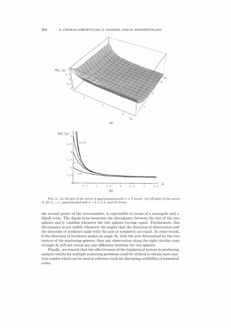
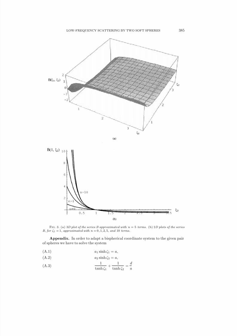
In accord with the theory of multiple scattering [9, 10], all the results obtained forthe near and the far fields are expressed in a series form which confirms the multipleinteraction between each one of the spheres and the field scattered from the order.Since we solve the problem analytically without any computational error, all ordersof the multiple scattering processes [9, 10] are included. Nevertheless, as shown inFigures 2 and 3, because of the exponential behavior of the terms defining the seriesA and B in (36), (84), and (85), the convergence is so fast that the restriction to twoleading terms alone derives results which are satisfactory for any practical purpose.
In the terminology of multiple scattering theory, this means that first-order mul-tiple scattering [9, 10] is enough for this particular problem. Hence, for practicalapplications it is enough to consider as an incident field impinging on each one of thespheres the external illumination field plus the outcome of its first interaction withthe other sphere.
The leading approximation of the scattering amplitude is proportional to the firstpower of the wavenumber and is isotropic since it is expressible in terms of a monopoleterm. The next approximation of the scattering amplitude, which is proportional to
7/31/2019 30408 two sph
http://slidepdf.com/reader/full/30408-two-sph 15/17
384 A. CHARALAMBOPOULOS, G. DASSIOS, AND M. HADJINICOLAOU
FIG. 2. (a) 3D plot of the series A approximated with n = 5 terms. (b) 2D plots of the series
A, for ζ 1 = 1, approximated with n = 0, 1, 2, 5, and 10 terms.
the second power of the wavenumber, is expressible in terms of a monopole and adipole term. The dipole term measures the discrepancy between the size of the twospheres and it vanishes whenever the two spheres become equal. Furthermore, thisdiscrepancy is not visible whenever the angles that the direction of observation andthe direction of incidence make with the axis of symmetry are equal. In other words,if the direction of incidence makes an angle θ0 with the axis determined by the twocenters of the scattering spheres, then any observation along the right circular coneof angle θ0 will not reveal any size difference between the two spheres.
Finally, we remark that the effectiveness of the bispherical system in producinganalytic results for multiple scattering problems could be utilized to obtain more ana-lytic results which can be used as reference tools for discussing credibility of numericalcodes.
7/31/2019 30408 two sph
http://slidepdf.com/reader/full/30408-two-sph 16/17
LOW-FREQUENCY SCATTERING BY TWO SOFT SPHERES 385
FIG. 3. (a) 3D plot of the series B approximated with n = 5 terms. (b) 2D plots of the series
B, for ζ 1 = 1, approximated with n = 0, 1, 2, 5, and 10 terms.
Appendix. In order to adapt a bispherical coordinate system to the given pairof spheres we have to solve the system
a1 sinh ζ 1 = a,(A.1)
a2 sinh ζ 2 = a,(A.2)
1
tanh ζ 1+
1
tanh ζ 2=
d
a(A.3)
7/31/2019 30408 two sph
http://slidepdf.com/reader/full/30408-two-sph 17/17
386 A. CHARALAMBOPOULOS, G. DASSIOS, AND M. HADJINICOLAOU
with respect to the unknowns a, ζ 1, and ζ 2. Equations (A.1), (A.2) imply
cosh ζ 1 =
1 +
a2
a21,(A.4)
cosh ζ 2 =
1 +
a2
a22.(A.5)
Substituting (A.1), (A.2), (A.4), and (A.5) into (A.3) we arrive at a21 + a2 +
a22 + a2 = d(A.6)
or, after eliminating the square roots,
4d2a2 = d4 + (a21 − a22)2 − 2d2(a21 + a22) = [d2 − (a1 − a2)2][d2 − (a1 + a2)2],(A.7)
which implies (7).
From (A.1), (A.2) we obtain
ζ i = sinh−1a
ai= ln
a +
a2 + a2iai
, i = 1, 2.(A.8)
Finally, substituting (7) into (A.8) for i = 1 and 2, we obtain (8) and (9), respectively.
REFERENCES
[1] J. J. BOWMAN, T. B. A. SENIOR, AND P. L. E. USLENGHI, Electromagnetic and Acoustic
Scattering by Simple Shapes, North-Holland, Amsterdam, 1969.[2] D. COLTON AND R. KRESS, Integral Equation Methods in Scattering Theory , John Wiley, New
York, 1983.[3] D. COLTON AND R. KRESS, Inverse Acoustic and Electromagnetic Scattering Theory , Springer-
Verlag, Berlin, 1992.[4] G. DASSIOS AND R. E. KLEINMAN, On Kelvin inversion and low-frequency scattering , SIAM
Rev., 31 (1989), pp. 565–585.[5] G. DASSIOS AND R. E. KLEINMAN, Low-frequency scattering by targets above a ground plane,
in Proc. 583 Advisory Group for Aerospace Research and Development Meeting on RadarSingature Analysis and Imaging of Military Targets, Ankara, Turkey, 1996, pp. 4-1–4-10.
[6] P. MOON AND D. E. SPENCER, Field Theory Handbook , Springer-Verlag, Berlin, 1961.[7] P. MOON AND D. E. SPENCER, Field Theory for Engineers, Van Nostrand, Princeton, 1961.[8] P. M. MORSE AND H. FESHBACH, Methods of Theoretical Physics, Vols. I, II, McGraw–Hill,
New York, 1953.[9] V. TWERSKY, Multiple scattering by arbitrary configuration in three dimensions, J. Math.
Phys., 3 (1962), pp. 83–91.[10] V. TWERSKY, Multiple scattering of electromagnetic waves by arbitrary configurations,
J. Math. Phys., 8 (1967), pp. 589–610.