3-DIMENSIONAL NUMERICAL MODELING OF AN · PDF fileheating systems, using the wave equation...

International Microwave Power Institute 87

T.V. Chow Ting Chan, J. Tang and F. Younce

Biological Systems Engineering Dept. Washington State University, Pullman, WA 99164-6120

This paper presents a new, yet simple and effective approach to modeling industrial Radio Frequency heating systems, using the wave equation applied in three dimensions instead of the conventional electrostatics method. The central idea is that the tank oscillatory circuit is excited using an external source. This then excites the applicator circuit which is then used to heat or dry the processed load. Good agreement was obtained between the experimental and numerical data, namely the S11-parameter, phase, and heating patterns for different sized loads and positions.

Submission Date: April, 2004Acceptance Date: October, 2004

3-DIMENSIONAL NUMERICAL MODELING OF AN INDUSTRIAL RADIO FREQUENCY HEATING SYSTEM

USING FINITE ELEMENTS

Keywords: Radio Frequency Heating, Computer Modeling, Finite Elements

Introduction

Industrial Radio Frequency (RF) heating systems, operating in the ISM (Industrial Scientific Medical) frequency bands at 13.56 MHz, 27.12 MHz, and 40.68 MHz, are a well-established method for processing various types of non-food materials, including textile and paper drying, plastics welding, and curing glue in plywood. Industrial applications can also be found in drying operations for food products, e.g., drying bakery products after baking processes [Metaxas and Clee, 1993; Metaxas, 1996a]. There is also a strong interest in using RF energy to preserve packaged foods [Wang et al., 2003a], or to control insect pests in agricultural commodities [Wang et al., 2002; Ikediala et al., 2002; Wang et al., 2003c].

Because of its long wavelength, RF energy penetrates dielectric materials deeper than microwaves. But the loss factor of most moist

foods, especially those containing high salt contents, increases with product temperature in the RF frequency range [Wang et al., 2003b; Guan et al., 2004]. This may lead to significant non-uniform heating.

It is, therefore, critical to design applicators that provide uniform RF field patterns in foods, and thereby overcoming the possibility of thermal runaway in moist foods containing dissolved salts [Wang et al., 2003a]. In current practice, experienced manufacturers often rely on intuition to build systems that meet their customers’ needs. In fact, most of the industrial RF systems are normally “designed” using trial and error by experienced people used to working with RF systems. Generally, time and money are wasted in troubleshooting and modifying the systems if they do not meet the design requirements. Computer simulation can play an important role in facilitating the design of RF heating systems. Although simulation, as such, cannot replace experimental work, it nevertheless can provide valuable information such as the electric field pattern in an applicator

88 Journal of Microwave Power & Electromagnetic Energy Vol. 39, No. 2, 2004 International Microwave Power Institute 89

with specific loads to guide the design of a new system.

An extensive literature survey of work done in the area of modeling has been described in Neophytou and Metaxas [1998]. Very good work has also been published by the same authors [Neophytou and Metaxas, 1996b, 1997, and 1999a] that lays the background for using a 3-D approach to modeling RF heating systems, i.e. by considering the combined tank and applicator circuits. Most of the simulation work prior to the above publications is based on the assumption of quasi-static conditions. A justification for this approach is that the RF wavelengths are large, in the order of meters, compared to the applicator cavity size which is only a fraction of a wavelength. Therefore, the Laplace equation is used to calculate the electromagnetic fields within the applicator and modeled independently of the generator unit, by using simplified one or two dimensional models. Metaxas and his co-author have found that there are, however, certain limitations in modeling RF heating systems by simply using one or two dimensional quasi-static models. Although, the quasi-static assumption was found to work in very small-sized applicators, an accurate prediction of the electromagnetic distribution in an RF applicator can only be obtained by modeling the complete system (tank and applicator) in three dimensions using the wave equation.

A challenge in using a computer to model RF systems is to validate the simulated results with experiments. This is undeniably the most difficult part for any research group working on simulation, whether it is in microwave or RF heating. Until good agreement is shown between the experimental and simulated results, simulation can provide little insight into the RF heating process and cannot be used in designing RF heating systems. Much less, it will be impossible to convince an audience of its usefulness.

The objective of our research was to develop a method of modeling RF heating systems. The

idea behind the method is to model the entire system, tank and applicator included. Although the combined system has been investigated by Neophytou and Metaxas [1999a], the latter only considered the eigenmodes, i.e. the natural resonances, within the system. This paper considers the combined system with the addition of a means of excitation to the tank oscillatory circuit with an external, properly positioned coaxial source. In so doing, the S11-parameter and phase of the combined tank and applicator circuits can be derived and compared with experimental work using a network analyzer. There may be other ways to model industrial RF heating systems; this paper, however, presents a way to visualize the heating pattern inside the load. Once correlated data has been obtained, it is then possible to study and understand the complex interaction between the RF field and the load. Designing new RF systems can then emanate from this understanding.

Various commercial packages such as HFSS® from Ansoft (Pitts, PA, USA); FEMLAB® from Comsol (Los Angeles, CA, USA); ANSYS® from Ansys Corp. (Canonsburg, PA, USA), CST Microwave Studio from CST (Darmstadt, Germany) can be used to model an RF system with varying degrees of success. In this paper, HFSS® was arbitrarily chosen.

Governing Equations

The governing equations in calculating the electromagnetic field inside an RF heating system are described by Maxwellʼs equations:

∇ = − ∂∂

x E Hµt (1)

∇ = ′ ∂

∂+

x H Eε ε σ0 r t (2)

∇ =• H 0 (3)

∇ =• D ρ (4)


where E is the electric field strength and H is the magnetic field strength. D is the electric flux density, ρ is the charge density, µ is the permeability, εo is the permittivity of free space (8.854×10-12 F/m), εrʹ is the relative dielectric constant, and σ is the effective (conductive and dipolar) conductivity.

If the fields are assumed to be time-harmonics, the following wave equation is obtained after manipulation of equations 1 and 2:

∇

′∇ − =x x E E1 02

µε

rrk

(5)

where k20 0= ω µ ε and ε ε σ ε ωr r OJ= ′ − / , μʹ

0 is

the relative permeability, μ0 is the permeability

of free space, and ω = 2πf represents the angular frequency of the waves.

In modeling an RF heating system, normally, the predicted variable from equation 5 is the electric field, from which the power density is computed knowing the effective loss factor. Since the main purpose of this paper

is to emphasize the use of a 3-D simulated model to predict the general heating pattern obtained during experiment, only a qualitative comparison, i.e. simulated electric field and experimental temperature patterns, has been provided. Heat transfer has not been incorporated in the simulated model as it was deemed unnecessary for the purpose of our investigation at this stage.

Industrial RF Heating System

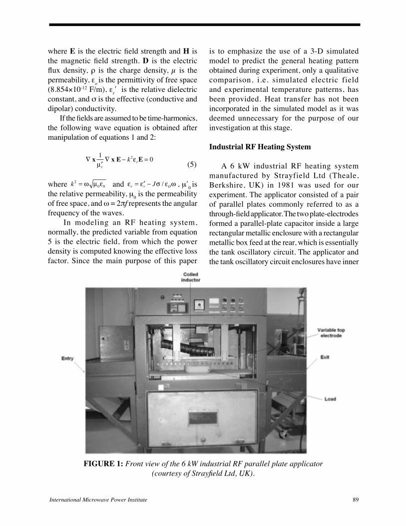
A 6 kW industrial RF heating system manufactured by Strayfield Ltd (Theale, Berkshire, UK) in 1981 was used for our experiment. The applicator consisted of a pair of parallel plates commonly referred to as a through-field applicator. The two plate-electrodes formed a parallel-plate capacitor inside a large rectangular metallic enclosure with a rectangular metallic box feed at the rear, which is essentially the tank oscillatory circuit. The applicator and the tank oscillatory circuit enclosures have inner

FIGURE 1: Front view of the 6 kW industrial RF parallel plate applicator (courtesy of Strayfield Ltd, UK).


dimensions of 120 x 65 x 75 cm3 and 56.2 x 58.6 x 50.4 cm3, respectively.

The top plate electrode of the applicator, with adjustable height, was inductively coupled to the tank oscillator circuit via a rectangular coaxial feed. The bottom side of the enclosure acted as the other electrode. With proper matching, the energy from the RF power unit which contained the tank oscillatory circuit was optimally transferred to the processed material between the movable top and fixed bottom plates, situated at the center of the enclosure. The load placed between the electrodes essentially became an

integral part of the applicator circuit.The top plate was also connected to a coiled

inductor (see Figure 1) to tune the applicator circuit to the intended operating frequency of 27.12 MHz. The required inductance depends on the dielectric properties and geometry of the load. The coiled inductor is not a common feature of RF applicators, but it can influence the heating pattern. If properly positioned, it can improve the heating uniformity.

A schematic view illustrating the equivalent electric circuit of the RF system is shown in Figure 2. It is basically a self-excited oscillatory

FIGURE 2: Equivalent electric circuit for the industrial RF heating system of Figure 1 without the coiled inductor (Courtesy of Strayfield Ltd, UK)


circuit system, typical of most RF systems on the market. Capacitor CAP3 and inductor IND1 form part of the tank oscillatory circuit, and inductor IND2 with the load form part of the applicator circuit. IND2 is essentially a pick-up inductor linked to the top plate of the applicator. The coiled inductor, not shown in the schematic, also forms part of the applicator circuit. CAP2 are two blocking anode capacitors having a value of 500pF each. The high voltage (6 kV d.c) is fed through a feed-through capacitor CAP1 to the triode valve. Capacitors CAP 4 to 7 and inductor IND3 form part of the oscillatory circuit.

Materials and Methods

Sample Preparation and Physical Characteristics

The material used for the study is CarboxyMethylCellulose (CMC) powder (pre-hydrated CMC 6000 powder, TIC Gums Inc., Belcamp, MD, USA). CMC is used because the material is very consistent over the working temperature range of our experiment, typically from 20oC to 80oC. It can, therefore, be used as a good model to compare simulation and experimental results. The test load is prepared by mixing CMC powder with water. The addition of CMC powder to water primarily changes the

dielectric loss factor, conductivity and viscosity depending on the concentration of the added CMC.

For this experiment, 1 % of CMC powder was used. If less than 1% of CMC powder is used, the viscosity of the solution would be very low at room temperature. After RF heating, the viscosity would be even less and would be difficult to handle because of its fluidity, especially when removing it from the system for infrared thermal camera measurement, described later in this paper. Low viscosity of the CMC solution might also result in natural convection in the load caused by possible non-uniform heating and the measured temperature pattern might not reflect the RF field pattern. After the solution was prepared, it was left for 24 hours to remove all the bubbles that were formed by mixing the CMC with water.

Dielectric Properties Measurement of 1% CarboxyMethylCellulose (CMC) Solution

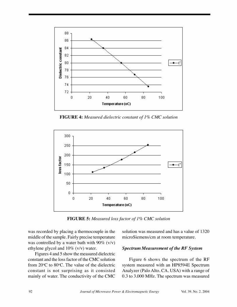
Figure 3 shows the dielectric properties measurement setup for the CMC solution. It consisted of an HP4291B Impedance Analyzer (Palo Alto, CA, USA), an HP85070B dielectric probe kit, and a custom-built test cell, in which the CMC solution was placed. The setup can measure material properties over a frequency range of 10 to 1,800 MHz. The temperature

FIGURE 3: Dielectric property measurement setup [Wang et al., 2003c]


was recorded by placing a thermocouple in the middle of the sample. Fairly precise temperature was controlled by a water bath with 90% (v/v) ethylene glycol and 10% (v/v) water.

Figures 4 and 5 show the measured dielectric constant and the loss factor of the CMC solution from 20oC to 80oC. The value of the dielectric constant is not surprising as it consisted mainly of water. The conductivity of the CMC

solution was measured and has a value of 1320 microSiemens/cm at room temperature.

Spectrum Measurement of the RF System

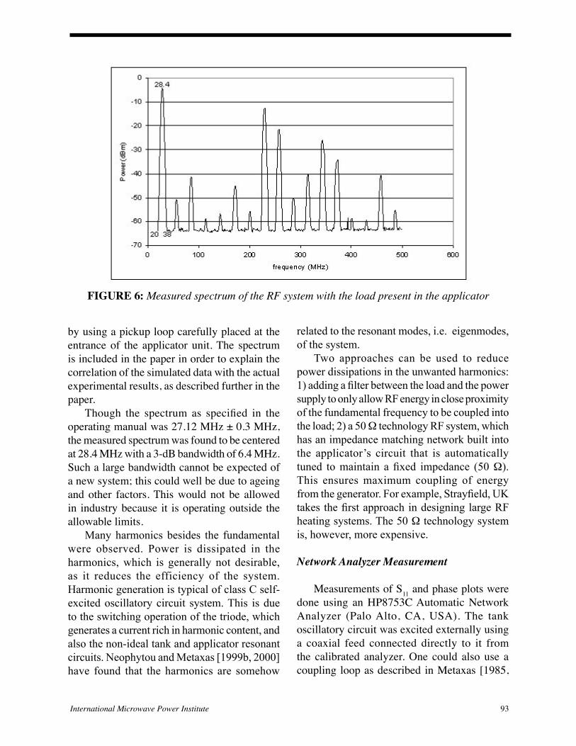
Figure 6 shows the spectrum of the RF system measured with an HP8594E Spectrum Analyzer (Palo Alto, CA, USA) with a range of 0.3 to 3,000 MHz. The spectrum was measured

FIGURE 4: Measured dielectric constant of 1% CMC solution

FIGURE 5: Measured loss factor of 1% CMC solution


by using a pickup loop carefully placed at the entrance of the applicator unit. The spectrum is included in the paper in order to explain the correlation of the simulated data with the actual experimental results, as described further in the paper.

Though the spectrum as specified in the operating manual was 27.12 MHz ± 0.3 MHz, the measured spectrum was found to be centered at 28.4 MHz with a 3-dB bandwidth of 6.4 MHz. Such a large bandwidth cannot be expected of a new system; this could well be due to ageing and other factors. This would not be allowed in industry because it is operating outside the allowable limits.

Many harmonics besides the fundamental were observed. Power is dissipated in the harmonics, which is generally not desirable, as it reduces the efficiency of the system. Harmonic generation is typical of class C self-excited oscillatory circuit system. This is due to the switching operation of the triode, which generates a current rich in harmonic content, and also the non-ideal tank and applicator resonant circuits. Neophytou and Metaxas [1999b, 2000] have found that the harmonics are somehow

related to the resonant modes, i.e. eigenmodes, of the system.

Two approaches can be used to reduce power dissipations in the unwanted harmonics: 1) adding a filter between the load and the power supply to only allow RF energy in close proximity of the fundamental frequency to be coupled into the load; 2) a 50 Ω technology RF system, which has an impedance matching network built into the applicator’s circuit that is automatically tuned to maintain a fixed impedance (50 Ω). This ensures maximum coupling of energy from the generator. For example, Strayfield, UK takes the first approach in designing large RF heating systems. The 50 Ω technology system is, however, more expensive.

Network Analyzer Measurement

Measurements of S11 and phase plots were done using an HP8753C Automatic Network Analyzer (Palo Alto, CA, USA). The tank oscillatory circuit was excited externally using a coaxial feed connected directly to it from the calibrated analyzer. One could also use a coupling loop as described in Metaxas [1985,

FIGURE 6: Measured spectrum of the RF system with the load present in the applicator


1987], and Neophytou and Metaxas [1997]. Unlike direct coupling, the coupling loop has the obvious advantage that it does not load the system. In our experiment, direct connection using an N-type connector to the tank circuit was found to work relatively well and did not affect the system significantly.

Special care is, however, required with regards to the feeding pointʼs location as the position of the direct feeding point using the coaxial feed will affect the degree of coupling and hence will have an effect on the S11-parameter. Improper coupling position could lead to high reflection, and therefore minimal or no power is coupled to the tank and applicator

circuit. For different RF systems, different feed locations will most likely be required.

Numerical Modeling of the Through-field RF Industrial Heating System

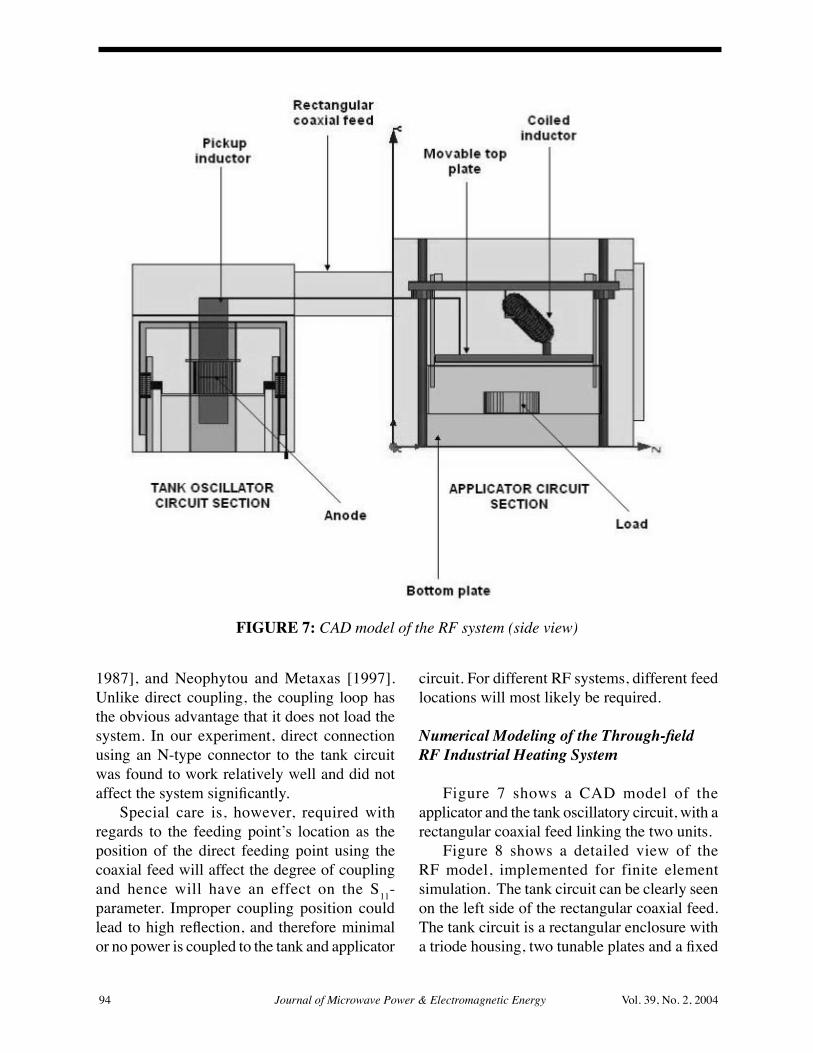
Figure 7 shows a CAD model of the applicator and the tank oscillatory circuit, with a rectangular coaxial feed linking the two units.

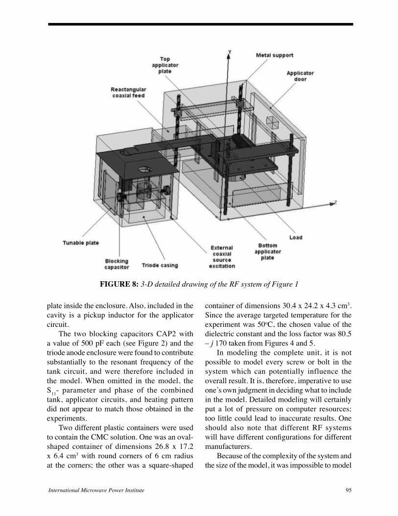
Figure 8 shows a detailed view of the RF model, implemented for finite element simulation. The tank circuit can be clearly seen on the left side of the rectangular coaxial feed. The tank circuit is a rectangular enclosure with a triode housing, two tunable plates and a fixed

FIGURE 7: CAD model of the RF system (side view)


plate inside the enclosure. Also, included in the cavity is a pickup inductor for the applicator circuit.

The two blocking capacitors CAP2 with a value of 500 pF each (see Figure 2) and the triode anode enclosure were found to contribute substantially to the resonant frequency of the tank circuit, and were therefore included in the model. When omitted in the model, the S11- parameter and phase of the combined tank, applicator circuits, and heating pattern did not appear to match those obtained in the experiments.

Two different plastic containers were used to contain the CMC solution. One was an oval-shaped container of dimensions 26.8 x 17.2 x 6.4 cm3 with round corners of 6 cm radius at the corners; the other was a square-shaped

container of dimensions 30.4 x 24.2 x 4.3 cm3. Since the average targeted temperature for the experiment was 50oC, the chosen value of the dielectric constant and the loss factor was 80.5 – j 170 taken from Figures 4 and 5.

In modeling the complete unit, it is not possible to model every screw or bolt in the system which can potentially influence the overall result. It is, therefore, imperative to use oneʼs own judgment in deciding what to include in the model. Detailed modeling will certainly put a lot of pressure on computer resources; too little could lead to inaccurate results. One should also note that different RF systems will have different configurations for different manufacturers.

Because of the complexity of the system and the size of the model, it was impossible to model

FIGURE 8: 3-D detailed drawing of the RF system of Figure 1


such system on a regular PC. Simulated model was done on a Hewlett-Packard workstation consisting of two 1.3 GHz Itanium CPUs and 8 G of RAM. The average number of tetrahedra for convergence for each model is around 180,000.

Neophytou and Metaxas [1998] considered in their paper the impedance of a prototype applicator to correlate their experimental results with the simulations. Other significant parameters that can give us valuable insight into the overall system are: S-parameters, VSWR, and phase. In this paper, two parameters, namely the S11-parameter and the phase are considered, in addition to the field patterns.

Results and Discussions

S11 -Parameter and Phase

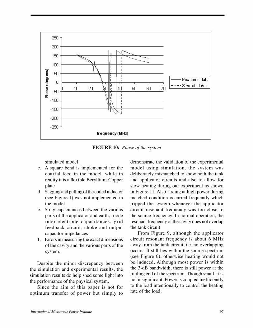
Figures 9 and 10 show the simulated and experimental S11 and phase plots of the oval container filled with CMC solution located at

the center of the applicator. Similar validation results were also done for the other load size and positions. As one would expect, the first peak is due to the physical dimensions of the coaxial tank circuit when energized by RF energy. It essentially establishes the operating frequency of the RF source. The second resonance is due to the applicator circuit.

A fairly good agreement was observed between the simulated and measured results of the S11-parameter and phase plots. The difference between the simulated and measured resonant frequencies was about 8 %. Ideally, it would be nice to have a perfect match between the simulated and experimental data. This is, however, unrealistic because it is impossible to include every physical feature in the simulation model. In particular, the discrepancy in the simulated and experimental S11 and phase plots can be attributed to a combination of any of the following:

a. Numerical errorsb. Non-inclusion of pins and screws in the

FIGURE 9: S11 of the tank and applicator circuit


FIGURE 10: Phase of the system

simulated modelc. A square bend is implemented for the

coaxial feed in the model, while in reality it is a flexible Beryllium-Copper plate

d. Sagging and pulling of the coiled inductor (see Figure 1) was not implemented in the model

e. Stray capacitances between the various parts of the applicator and earth, triode inter-electrode capacitances, grid feedback circuit, choke and output capacitor impedances

f. Errors in measuring the exact dimensions of the cavity and the various parts of the system.

Despite the minor discrepancy between the simulation and experimental results, the simulation results do help shed some light into the performance of the physical system.

Since the aim of this paper is not for optimum transfer of power but simply to

demonstrate the validation of the experimental model using simulation, the system was deliberately mismatched to show both the tank and applicator circuits and also to allow for slow heating during our experiment as shown in Figure 11. Also, arcing at high power during matched condition occurred frequently which tripped the system whenever the applicator circuit resonant frequency was too close to the source frequency. In normal operation, the resonant frequency of the cavity does not overlap the tank circuit.

From Figure 9, although the applicator circuit resonant frequency is about 6 MHz away from the tank circuit, i.e. no overlapping occurs. It still lies within the source spectrum (see Figure 6), otherwise heating would not be induced. Although most power is within the 3-dB bandwidth, there is still power at the trailing end of the spectrum. Though small, it is not insignificant. Power is coupled inefficiently to the load intentionally to control the heating rate of the load.


FIGURE 11: Measured temperature using 3 fiber-optic probes

Temperature changes of the CMC solution

Fiber-optic temperature probes (FISO Technologies Inc., Quebec, Canada) connected to a computer were used to record temperatures at three different points inside the CMC solution. An arbitrary average target temperature of 50oC was chosen to stop the experiment. The temperature recorded gave a qualitative indication of the load temperature at which the system should be turned off and the load removed for thermal camera measurement. Obviously, placing the probes at other locations will indicate different temperature measurements.

Heating Patterns

Although the fiber-optic probes are generally reliable and give reasonably accurate indication of the hot and cold regions inside the load, the logistics of measuring temperature at each point inside the load is overwhelming. An infrared thermal camera model ThermaCam SC300 with an accuracy of ±2oC and 5 picture recordings per second [Flir Systems, Portland, Oregon] was used to measure the surface temperature

profile. Although the camera could only record the surface temperature, this information is useful to validate the surface pattern predicted by the model. Once validated, the model can then be used to determine the heating pattern inside the load.

Figures 12 to 16 show a very good comparison between the measured temperature patterns and predicted RF electric field patterns for five different load positions and container sizes. Top views of the RF system showing the relative positions of the load inside the applicator for the various scenarios are also given.

The heating spots at the right side of Figure 12a and the top left corner of Figure 13a are due to handling the container immediately after removal from the applicator. From Figures 12 and 16, as one would expect, container size, shape and position influence the heating pattern. Notable observations from Figures 12 to 15 are that heating primarily occurs on the edge of the container. In Figure 16, since part of the container lies outside of the plate, no heating could be expected.

The material properties for the 1% CMC solution used in the simulation are for 50oC.


a)

b)

FIGURE 12: a) Measured temperature of the 1% CMC solution in the oval container at the center of the applicator; b) simulated electric

field of the 1% CMC solution in the oval container at the center of the applicator


FIGURE 13: (a) Measured temperature of the 1% CMC solution in the oval container at the center of the applicator, but rotated by 90o,

(b) simulated electric field of the 1% CMC solution in the oval container at the center of

the applicator, but rotated by 90o

a)

b)


a)

b)

FIGURE 14: (a) Measured temperature of the 1% CMC solution in the rectangular container, (b) simulated electric field of the

1% CMC solution in the rectangular container


a)

b)

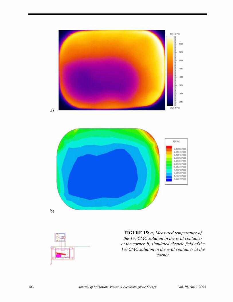
FIGURE 15: a) Measured temperature of the 1% CMC solution in the oval container

at the corner, b) simulated electric field of the 1% CMC solution in the oval container at the

corner


FIGURE 16: (a) Measured temperature of the 1% CMC solution in the offset oval container,

b) simulated electric field of the 1% CMC solution in the offset oval container

a)

b)


Since the fiber-optic probes recorded the temperature inside the load, it could be that the surface temperature exceeded 50oC, which would explain the discrepancy between the heating patterns for the simulation and experiment. Nevertheless, the computer simulation model predicted very well the general field patterns in the CMC load. It can be used to guide the design of new RF applicators in on-going efforts to develop RF sterilization and pasteurization technologies for industrial heating applications currently undertaken at Washington State University.

Conclusions

This paper demonstrates the ability of an RF model to effectively simulate an actual RF system. The model uses an Automatic Network Analyzer and a thermal camera for experimental work, and finite elements for numerical simulations. Once the model is validated, the heating pattern can then be observed with confidence and changes be made to the system to alter the pattern for better heating uniformity.

In the industry, most people rely on their vast experience they have acquired while working with RF systems. While it is undeniable that simulation cannot replace experience, one would certainly agree that a good simulation platform definitely adds value and credibility to the design of RF systems.

Acknowledgements

The work is supported by funding from the US Army Natick Soldier Center, Natick, MA, USA and by Washington State University Agricultural Research Center. We acknowledge technical advise of Tony Koral from Strayfield Ltd, UK and for granting us the use of the industrial RF system. We thank Mr. Wayne Dewitt for providing us with technical support.

References

Guan, D., Cheng, M., Wang, Y., Tang, J. (2004). Dielectric Properties of Mashed Potatoes Relevant to Microwave and Radio-Frequency Pasteurization and Sterilization Processes. J. Food Sci. 69(1): 30-37.

Ikediala, J.N., Hansen, J., Tang, J., Drake, S.R., Wang, S. (2002). Quarantine Treatment of Cherries Using Radio Frequency Energy and Saline-water-immersion Technique. Post-harvest Biology and Technology 24(1): 25-37.

Metaxas, A.C. (1985). Network Analysis on Radio Frequency Prototype Industrial Applicators. J Microwave Power: 20 (4), 197-216.

Metaxas, A.C. (1987). The Dynamic Impedance of Radio Frequency Heating Generators. J Microwave Power and Electromagnetic Energy: 22(3),127-136.

Metaxas, A.C., & Clee, M. (1993). Coupling and Matching of Radio Frequency Industrial Applicators. IEE Power Engineering Journal, 7(2): 85-93.

Metaxas, A.C. (1996a). Foundations of Electroheat, A Unified Approach, John Wiley and Sons, USA.

Neophytou, R.I., & Metaxas, A.C. (1996b). Computer Simulation of a Radio Frequency Industrial System. J Microwave Power and Electromagnetic Energy 31 (4):251-259.

Neophytou, R.I., & Metaxas, A.C. (1997). Characterisation of Radio Frequency Heating Systems in Industry Using a Network Analyzer. IEE Proc.-Sci. Meas. Technol, 144 (5):215-222.

Neophytou, R.I., & Metaxas, A.C. (1998). Combined 3D FE and Circuit Modeling of Radio Frequency Heating Systems. J Microwave Power and Electromagnetic Energy 33 (4):243-262.

Neophytou, R.I., & Metaxas, A.C. (1999a). Combined Tank and Applicator Design of Radio Frequency Heating Systems. IEE Proc.-Microw. Antennas Propag. 146 (5), 311-318.

Neophytou, R.I., & Metaxas, A.C. (1999b). Investigation of the Harmonic Generation in Conventional Radio Frequency Heating Systems. J Microwave Power and Electromagnetic Energy 34 (2):84-96.

Neophytou, R.I., & Metaxas, A.C. (2000).


Determination of Resonant Modes of RF Heating Systems Using Eigenvalue Analysis. J Microwave Power and Electromagnetic Energy 35 (1):1-14.

Wang, S., Tang, J., Johnson, J., Mitcham, B., and Hansen, J. (2002). Process Protocols Based on Radio Frequency Energy to Control Field and Storage Pests in In-shell Walnuts. Postharvest Biology and Technology 26(3): 265-273.

Wang, Y., Wig, T., Tang, J, and Hallberg, L.M. (2003a). Sterilization of Foodstuffs using Radio Frequency Heating. J. Food Sci. 68(2): 539-544.

Wang, Y., Wig, T., Tang, J, and Hallberg, L.M. (2003b). Dielectric Properties of Food Relevant to RF and Microwave pasteurization and Sterilization. J. Food Engineering 57 (3): 257-268.

Wang, S. Tang, J., Cavalieri, R., Davis, D. (2003c). Differential Heating of Insects Pests in Walnuts in RF and Microwave Treatments, Trans. ASAE 46(4): 1175-1182.

106 Journal of Microwave Power & Electromagnetic Energy Vol. 39, No. 2, 2004

3-DIMENSIONAL NUMERICAL MODELING OF AN · PDF fileheating systems, using the wave equation...

Documents

Transcript of 3-DIMENSIONAL NUMERICAL MODELING OF AN · PDF fileheating systems, using the wave equation...