2A.4 Refining CAM-based Tornado Probability Forecasts ...2A.4 Refining CAM-based Tornado Probability...
5
2A.4 Refining CAM-based Tornado Probability Forecasts Using Storm-inflow and Storm-attribute Information David E. Jahn 1,2* , Burkely T. Gallo 1,2 , Chris Broyles 2 , Bryan T. Smith 2 , Israel Jirak 2 , Jeffrey Milne 1,2 1 Cooperative Institute for Mesoscale Meteorological Studies/University of Oklahoma, Norman, OK 2 Storm Prediction Center/NWS/NOAA, Norman, OK 1. INTRODUCTION With the real-time operational implementation of convective-allowing models (CAMs) having spatial resolution of 3 – 4 km, effort has been given among the weather research community to identify signatures from simulated storms to differentiate environments that favor tornadic storms. This relatively high spatial resolution is insufficient to resolve tornadogenesis explicitly; however, the attributes of resolved individual storms and storm complexes as proxies of tornado development have been studied. For example, Thompson et al. (2003, 2012) formulated a single parameter that combines values of select environmental attributes that favor tornadic storms, namely the Significant Tornado Parameter (STP). The STP accounts for environmental instability, convective inhibition, wind speed and directional shear, as well as lifting condensation level of the near-storm environment. Favorable tornado environments can be assessed by calculating STP based on CAM forecasts of these fields. Thompson et al. (2017) documented a near-linear relationship among STP values and tornado frequency (Fig. 1) by calculating STP for the near-storm environment of more than 6,500 right-moving supercell storms associated with a severe report (not all tornadic) observed over a two-year period, 2014 – 15. In addition to forecasting environmental characteristics, CAMs are able to predict storm attributes such as updraft helicity (UH), which has also been identified as a useful field for evaluating tornado potential (Kain et al., 2008; Clark et al., 2013). CAM-based mid-level storm rotation, represented by a vertically-integrated UH over a 2 – 5 km AGL layer, is shown to have a level of skill in distinguishing tornadic storms above the use of environmental parameters alone (Sobash et al. 2016, Gallo et al. 2016). Gallo et al. (2018) proposed a method (herein the “Gallo” method) to generate next-day probabilistic tornado guidance based on CAM forecasts of the near-storm environment (per a calculated STP) and storm attributes, specifically UH. Forecasts represent the probability of tornado occurrence within 40 km of a point and anytime in a 24-hour period beginning at 12 UTC of a given day. As detailed in Gallo et al. (2018), this method was designed using CAM forecasts of 4-km grid resolution that are initiated at 00 UTC. The Gallo method is comprised of three primary steps: 1) Consider only CAM model grid points with right-moving rotating storms such that UH is greater than or equal to a threshold value of 25 m 2 s -2 ; 2) For selected grid points, populate a distribution of STP values using data from surrounding points for which UH exceeds 25 m 2 s -2 within a circular sweep area of 40- km radius (Fig. 2) and from the previous forecast hour (the pre-storm environment); and, 0 5 10 15 20 25 30 35 40 45 50 0-0.9 1.0-1.9 2.0-2.9 3.0-3.9 4.0-4.9 5.0-5.9 6.0-6.9 Tornado Probability STP EF0+ EF2+ Figure 1. Derived from Thompson et al. (2017) showing relationship of STP and tornado probability for 6,500+ documented right-moving supercells. * Corresponding author address: David E. Jahn, CIMMS/Univ. of OK, 120 David L. Boren Blvd., Norman, OK 73072; e-mail: [email protected].
Transcript of 2A.4 Refining CAM-based Tornado Probability Forecasts ...2A.4 Refining CAM-based Tornado Probability...
2A.4 Refining CAM-based Tornado Probability Forecasts Using Storm-inflow and Storm-attribute Information
David E. Jahn 1,2*, Burkely T. Gallo1,2, Chris Broyles2, Bryan T. Smith2, Israel Jirak2, Jeffrey Milne1,2
1Cooperative Institute for Mesoscale Meteorological Studies/University of Oklahoma, Norman, OK 2Storm Prediction Center/NWS/NOAA, Norman, OK
1. INTRODUCTION
With the real-time operational implementation of convective-allowing models (CAMs) having spatial resolution of 3 – 4 km, effort has been given among the weather research community to identify signatures from simulated storms to differentiate environments that favor tornadic storms. This relatively high spatial resolution is insufficient to resolve tornadogenesis explicitly; however, the
attributes of resolved individual storms and storm complexes as proxies of tornado development have been studied. For example, Thompson et al. (2003, 2012) formulated a single parameter that combines values of select environmental attributes that favor tornadic storms, namely the Significant Tornado Parameter (STP). The STP accounts for environmental instability, convective inhibition, wind speed and directional shear, as well as lifting condensation level of the near-storm environment. Favorable tornado environments can
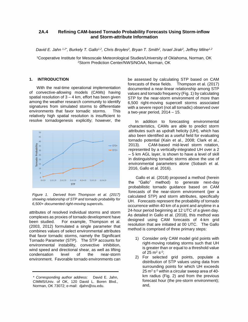
be assessed by calculating STP based on CAM forecasts of these fields. Thompson et al. (2017) documented a near-linear relationship among STP values and tornado frequency (Fig. 1) by calculating STP for the near-storm environment of more than 6,500 right-moving supercell storms associated with a severe report (not all tornadic) observed over a two-year period, 2014 – 15.
In addition to forecasting environmental characteristics, CAMs are able to predict storm attributes such as updraft helicity (UH), which has also been identified as a useful field for evaluating tornado potential (Kain et al., 2008; Clark et al., 2013). CAM-based mid-level storm rotation, represented by a vertically-integrated UH over a 2 – 5 km AGL layer, is shown to have a level of skill in distinguishing tornadic storms above the use of environmental parameters alone (Sobash et al. 2016, Gallo et al. 2016).
Gallo et al. (2018) proposed a method (herein the “Gallo” method) to generate next-day probabilistic tornado guidance based on CAM forecasts of the near-storm environment (per a calculated STP) and storm attributes, specifically UH. Forecasts represent the probability of tornado occurrence within 40 km of a point and anytime in a 24-hour period beginning at 12 UTC of a given day. As detailed in Gallo et al. (2018), this method was designed using CAM forecasts of 4-km grid resolution that are initiated at 00 UTC. The Gallo method is comprised of three primary steps:
1) Consider only CAM model grid points with right-moving rotating storms such that UH is greater than or equal to a threshold value of 25 m2 s-2;
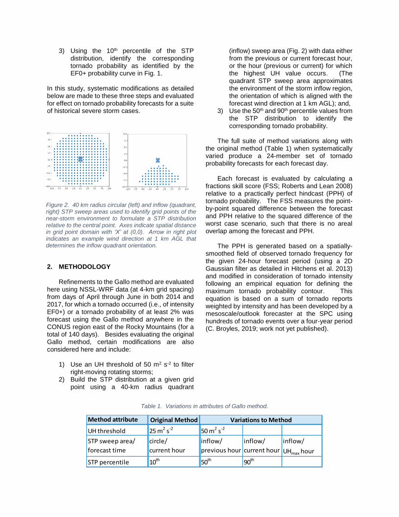
2) For selected grid points, populate a distribution of STP values using data from surrounding points for which UH exceeds 25 m2 s-2 within a circular sweep area of 40-km radius (Fig. 2) and from the previous forecast hour (the pre-storm environment); and,
0
5
10
15
20
25
30
35
40
45
50
0-0.9 1.0-1.9 2.0-2.9 3.0-3.9 4.0-4.9 5.0-5.9 6.0-6.9
Torn
ado
Pro
bab
ility
STP
EF0+
EF2+
Figure 1. Derived from Thompson et al. (2017)
showing relationship of STP and tornado probability for
6,500+ documented right-moving supercells.
* Corresponding author address: David E. Jahn,
CIMMS/Univ. of OK, 120 David L. Boren Blvd., Norman, OK 73072; e-mail: [email protected].
3) Using the 10th percentile of the STP distribution, identify the corresponding tornado probability as identified by the EF0+ probability curve in Fig. 1.
In this study, systematic modifications as detailed below are made to these three steps and evaluated for effect on tornado probability forecasts for a suite of historical severe storm cases.
2. METHODOLOGY
Refinements to the Gallo method are evaluated here using NSSL-WRF data (at 4-km grid spacing) from days of April through June in both 2014 and 2017, for which a tornado occurred (i.e., of intensity EF0+) or a tornado probability of at least 2% was forecast using the Gallo method anywhere in the CONUS region east of the Rocky Mountains (for a total of 140 days). Besides evaluating the original Gallo method, certain modifications are also considered here and include:
1) Use an UH threshold of 50 m2 s-2 to filter right-moving rotating storms;
2) Build the STP distribution at a given grid point using a 40-km radius quadrant
(inflow) sweep area (Fig. 2) with data either from the previous or current forecast hour, or the hour (previous or current) for which the highest UH value occurs. (The quadrant STP sweep area approximates the environment of the storm inflow region, the orientation of which is aligned with the forecast wind direction at 1 km AGL); and,
3) Use the 50th and 90th percentile values from the STP distribution to identify the corresponding tornado probability.
The full suite of method variations along with the original method (Table 1) when systematically varied produce a 24-member set of tornado probability forecasts for each forecast day.
Each forecast is evaluated by calculating a fractions skill score (FSS; Roberts and Lean 2008) relative to a practically perfect hindcast (PPH) of tornado probability. The FSS measures the point-by-point squared difference between the forecast and PPH relative to the squared difference of the worst case scenario, such that there is no areal overlap among the forecast and PPH.
The PPH is generated based on a spatially-smoothed field of observed tornado frequency for the given 24-hour forecast period (using a 2D Gaussian filter as detailed in Hitchens et al. 2013) and modified in consideration of tornado intensity following an empirical equation for defining the maximum tornado probability contour. This equation is based on a sum of tornado reports weighted by intensity and has been developed by a mesoscale/outlook forecaster at the SPC using hundreds of tornado events over a four-year period (C. Broyles, 2019; work not yet published).
Method attribute Original Method
UH threshold 25 m2 s-2 50 m2 s-2
STP sweep area/
forecast time
circle/
current hour
inflow/
previous hour
inflow/
current hour
inflow/
UHmax hour
STP percentile 10th 50th 90th
Variations to Method
Table 1. Variations in attributes of Gallo method.
Figure 2. 40 km radius circular (left) and inflow (quadrant, right) STP sweep areas used to identify grid points of the near-storm environment to formulate a STP distribution relative to the central point. Axes indicate spatial distance in grid point domain with ‘X’ at (0,0). Arrow in right plot indicates an example wind direction at 1 km AGL that determines the inflow quadrant orientation.
3. RESULTS
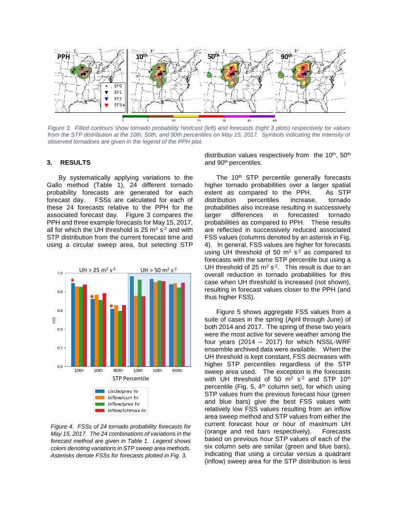
By systematically applying variations to the Gallo method (Table 1), 24 different tornado probability forecasts are generated for each forecast day. FSSs are calculated for each of these 24 forecasts relative to the PPH for the associated forecast day. Figure 3 compares the PPH and three example forecasts for May 15, 2017, all for which the UH threshold is 25 m2 s-2 and with STP distribution from the current forecast time and using a circular sweep area, but selecting STP
distribution values respectively from the 10th, 50th and 90th percentiles.
The 10th STP percentile generally forecasts higher tornado probabilities over a larger spatial extent as compared to the PPH. As STP distribution percentiles increase, tornado probabilities also increase resulting in successively larger differences in forecasted tornado probabilities as compared to PPH. These results are reflected in successively reduced associated FSS values (columns denoted by an asterisk in Fig. 4). In general, FSS values are higher for forecasts using UH threshold of 50 m2 s-2 as compared to forecasts with the same STP percentile but using a UH threshold of 25 m2 s-2. This result is due to an overall reduction in tornado probabilities for this case when UH threshold is increased (not shown), resulting in forecast values closer to the PPH (and thus higher FSS).
Figure 5 shows aggregate FSS values from a suite of cases in the spring (April through June) of both 2014 and 2017. The spring of these two years were the most active for severe weather among the four years (2014 – 2017) for which NSSL-WRF ensemble archived data were available. When the UH threshold is kept constant, FSS decreases with higher STP percentiles regardless of the STP sweep area used. The exception is the forecasts with UH threshold of 50 m2 s-2 and STP 10th percentile (Fig. 5, 4th column set), for which using STP values from the previous forecast hour (green and blue bars) give the best FSS values with relatively low FSS values resulting from an inflow area sweep method and STP values from either the current forecast hour or hour of maximum UH (orange and red bars respectively). Forecasts based on previous hour STP values of each of the six column sets are similar (green and blue bars), indicating that using a circular versus a quadrant (inflow) sweep area for the STP distribution is less
PPH 10th 50th 90th
Figure 3. Filled contours show tornado probability hindcast (left) and forecasts (right 3 plots) respectively for values from the STP distribution at the 10th, 50th, and 90th percentiles on May 15, 2017. Symbols indicating the Intensity of
observed tornadoes are given in the legend of the PPH plot.
Figure 4. FSSs of 24 tornado probability forecasts for
May 15, 2017. The 24 combinations of variations in the
forecast method are given in Table 1. Legend shows
colors denoting variations in STP sweep area methods.
Asterisks denote FSSs for forecasts plotted in Fig. 3.
STP Percentile
*
*
UH > 50 m2 s-2UH > 25 m2 s-2
*

a factor as compared to the relative forecast hour (previous or current) used to calculate STP.
The results of Fig. 5 are in consideration of observed tornadoes of any intensity, EF0+. Figure 6 gives aggregate FSSs across the same period (spring months of 2014 and 2017), but using PPH based on observed tornadoes of intensity EF2 and higher. Tornado probability forecasts are generated from CAM STP values using the EF2+ curve of Fig. 1. Results show a strong sensitivity to the STP percentile. FSS increases with higher STP percentile regardless of using a circular or inflow STP sweep area. Results are also less sensitive to UH threshold as compared to STP percentile.
The difference in FSS trends among Figs. 5 and 6 is striking when considering only observed tornadoes of intensity EF2 and greater. Tornado probabilities here are based on an empirical relationship of STP and tornado frequency strictly in consideration of right-moving rotating supercell storms (Thompson et al. 2017). However, the CAM-based tornado probabilities here do not filter out other storm modes that can produce tornadoes such as mesoscale convective systems (MCSs), nor are such systems filtered out of the tornado reports used here for verification. The STP-tornado probability EF0+ curve of Fig. 1 thus may not be appropriate for such subset of MCS-associated tornadoes here, which are generally of relatively low intensity (less than EF2) as compared to their supercell counterparts (Smith et al. 2012). This is less of a factor for tornado probabilities involving tornadoes of EF2 intensity and higher as shown in Fig. 6.
Toward improving tornado probabilities for
lower-end tornadoes (Fig. 1), research is on-going to develop methods to filter MCS-related UH in CAMs. Also, the relationship of STP and UH threshold values associated with tornadoes from MCSs is not known and would require further research.
4. SUMMARY
This study investigates the effect of various modifications to the Gallo method on tornado probability forecasts, which is a method dependent on CAM output fields associated with storm environment (i.e., STP) and storm attributes (i.e., UH). Modifications considered here include two different UH thresholds used to filter rotating storms, four different means for populating a STP distribution associated with the near-environment of a rotating storm, and selecting three different percentiles from the STP distribution to identify a single STP value for assigning a tornado probability at a given grid point of the domain. Systematically varying these set of modifications results in 24 forecasts for each forecast day. This approach is implemented for 140 forecast days occurring in the spring months of 2014 and 2017. Results show a primary sensitivity to STP percentile, with highest FSS values (best forecasts) when using the 10th STP percentile for tornadoes of any intensity. However, the best results for EF2+ tornadoes are given using the 90th percentile. Further work is required to identify causes for the different results
Figure 5. Same as Fig. 4, but showing aggregated results of 140 forecast days (see text).
STP Percentile
UH > 50 m2 s-2UH > 25 m2 s-2
Figure 6. Same as Fig. 5, but showing aggregated results in consideration only of tornadoes of intensity
EF2 and greater.
STP Percentile
UH > 50 m2 s-2UH > 25 m2 s-2
when filtering out low-intensity tornadoes. This discrepancy may be associated with non-supercell tornadoes. Acknowledgements This extended abstract was prepared by David Jahn with funding provided by NOAA/Office of Oceanic and Atmospheric Research under NOAA-University of Oklahoma Cooperative Agreement #NA16OAR4320115, U.S. Department of Commerce. The statements, findings, conclusions, and recommendations are those of the authors and do not necessarily reflect the views of NOAA or the U.S. Department of Commerce. References Clark, A. J., J. Gao, P. T. Marsh, T. Smith, J. S.
Kain, J. Correia, M. Xue, and F. Kong, 2013: Tornado pathlength forecasts from 2010 to 2011 using ensemble updraft helicity. Wea. Forecasting, 28, 387–407.
Gallo, B. T., A. J. Clark, B. T. Smith, R. L.
Thompson, I. Jirak, 2018: Blended probabilistic tornado forecasts: Combining climatological frequencies with NSSL-WRF ensemble forecasts. Wea. Forecasting, 33, 443-459.
Gallo, B. T., A. J. Clark, and S. R. Dembek, 2016:
Forecasting tornadoes using convection-
permitting ensembles. Wea. Forecasting, 31,
273–295.
Hitchens, N. M., H. E. Brooks and M. P. Kay, 2013:
Objective limits on forecasting skill of rare
events. Wea. Forecasting, 28, 525-534.
Kain, J. S., S. J. Weiss, D. R. Bright, M. E. Baldwin,
J. J. Levit, G. W. Cargin, C. S. Schwartz, M. L.
Weisman, K. K. Droegemeier, D. B. Weber, K.
W. Thomas, 2008: Some practical
considerations regarding horizontal resolution
in the first generation of operational convection-
allowing NWP. Wea. Forecasting, 23, 931–952
Roberts N. M., Lean H. W., 2008. Scale‐selective
verification of rainfall accumulations from high‐resolution forecasts of convective events. Mon.
Weather Rev. 136: 78– 97.
Smith, B. T., R. L. Thompson, J. S. Grams, and C.
Broyles, 2012: Convective modes for
significant severe thunderstorms in the
contiguous United States. Part I: Storm
classification and climatology. Wea.
Forecasting, 27, 1114-1135.
Sobash, R. A., G. S. Romine, C. S. Schwartz, D. J.
Gagne, and M. L. Weisman, 2016: Explicit
forecasts of low-level rotation from convection-
allowing models for next-day tornado
prediction. Wea. Forecasting, 31, 1591–1614
Thompson, R. L., B. T. Smith, J. S. Grams, A. R.
Dean, J. C. Picca, A. E. Cohen, E. M. Leitman,
A. M. Gleason, and P. T. Marsh, 2017:
Tornado damage rating probabilities derived
from WSR-88D data. Wea. Forecasting, 32,
1509-1528.
Thompson, R. L., B. T. Smith, J. S. Grams, A. R.
Dean, and C. Broyles, 2012: Convective
modes for significant severe thunderstorms in
the contiguous United States. Part II:
Supercell and QLCS tornado environments.
Wea. Forecasting, 27, 1136-1154.
Thompson, R. L., R. Edwards, J.A. Hart, K.L. Elmore and P.M. Markowski, 2003: Close proximity soundings within supercell environments obtained from the Rapid Update Cycle. Wea. Forecasting, 18, 1243–1261.