(a) ABB IRB 1206DOF robot arm.

(b) Atlas Humanoidrobot.

Figure 2.11: Fixed base (a) and floating base (b) systems.

2.8 Kinematics of Systems of BodiesMost robotic systems can be modeled as open kinematic structures composed of nl =nj + 1 links connected by nj joints (prismatic or revolute) with one degree of freedomeach. Since there is a single joint with displacement qi between two successive bodies,a simple transformation relates both bodies:

TBi−1Bi = TBi−1Bi (qi) (2.119)

There are two different types, namely fixed base and floating base systems wherebythe root link is either connected to the ground or freely moving. In the followingwhen discussing general aspects of multi-body kinematics we will focus on fixed basesystems such as manipulators. Floating base systems will be specifically covered insection 2.10. When dealing with fixed base systems, the frame attached to the root linkis often selected to be identical with the world fixed (inertial) frame.

2.8.1 Generalized Coordinates and Joint ConfigurationThe configuration of a robot such as a manipulator can be described by the generalizedcoordinate vector

q =

q1

...qn

. (2.120)

This set of scalar values must completely describe the configuration of the system,i.e. for constant values of q, the robot cannot move anymore. In most cases, onechooses coordinates that are independent, which implies that the number of generalizedcoordinates corresponds to the number of degrees of freedom. For a fixed base systemwithout additional kinematic constraints, this minimal set of generalized coordinatesare then called minimal coordinates. It is important to understand that the choice ofgeneralized coordinates is not unique. However, in most applications the generalizedcoordinates correspond to the degrees of freedom of the robot: For revolute joints, thesingle degree of freedom qi corresponds to the rotation angle of the joint. In case of aprismatic joint, qi represents the linear displacement.

29

eAy

eAz

eBxeBy

B

re

AeAx

eBz

Figure 2.12: Example of task space coordinates corresponding to the end-effector of amanipulator.

Example 2.8.1: Generalized Coordinates and Joint Configuration

The generalized coordinates of aSCARA robot arm are:

q =(α β γ ζ

)T, (2.121)

with the rotation angles α, β, and γaround the global vertical axis and thelinear displacement ζ.

2.8.2 Task-Space CoordinatesThe configuration of the end-effector of a robot arm as depicted in Fig. 2.12 can bedescribed by its relative position and orientation w.r.t. a reference frame. The referenceframe is often selected as the inertial or root frame.

End-Effector Configuration Parameters

As we have seen in section 2.2.1 and section 2.4.5, the position re ∈ R3 and rotationφe ∈ SO(3) of a frame with respect to a base can be parameterized byχP respectivelyχR. Hence, the combined position and orientation (of the end-effector) is given by

xe =

(reφe

)∈ SE(3), (2.122)

30

which can be parameterized by

χe =

(χePχeR

)=

χ1

...χm

∈ Rm. (2.123)

The number m varies depending on the parameterization. Please remember at thispoint that the rotation φe is only a theoretical abstraction of the orientation, for whichno numerical equivalent such as ”angular position” exists (see section 2.4).

Example 2.8.2: End-effector Configuration

To describe the end-effector in 3D space using Cartesian position parameters(3) as well as Euler Angles (3), gives a total of m = 6 parameters. In case oneuses spherical position parameters (3) and all elements of the direction cosinematrix associated with the rotation (9), m = 12 parameters will be necessary.

Operational Space Coordinates

The end-effector of a manipulator operates in the so-called operational space, whichdepends on the geometry and structure of the arm. The operational space can be de-scribed by

χo =

(χoPχoR

)=

χ1

...χm0

, (2.124)

whereby χ1, χ2, . . . , χm0are independent operational space coordinates1. Hence, they

can be understood as a minimal selection of end-effector configuration parameters.Note that m0 ≤ nj since the degree of mobility at the end-effector is certainly notlarger than the number of joints in the system.

Example 2.8.3: Operational Space Coordinates 1

To describe the end-effector in the most general case of a six-dimensional op-erational space requires m0 = 6 parameters. Hence, only Euler Angles are avalid parameterization while the choice of quaternions or rotation matrix is notpossible.

1Please note that there are different definitions for operational space coordinates in literature and someuse them as equivalent to end-effector coordinates. We introduce this here as minimal representation toproperly define things like e.g. singularities.

31

Example 2.8.4: Operational Space Coordinates 2

For a SCARA robot arm as depicted onthe left, the operational space is only4DOF, namely the three positions andthe rotation around the vertical axis.

χo =

xyzϕ

(2.125)

Note: In the example for the SCARA robot arm it is relatively simple to definefour operational space coordinates for a 4DOF arm. However, in case of an armwith four non co-linear rotation axes, it can be impossible to select four oper-ational space coordinates. In such an example, operational space coordinatesremain a rather theoretical concept.

In the following, we will not work with operational space coordinates but focus onthe more generic concept of end-effector configuration parameters.

2.8.3 Forward Kinematics

Forward kinematics describes the mapping between joint (generalized) coordinates qand the end-effector configuration χe:

χe = χe (q) . (2.126)

This relation can be obtained through the evaluation of (2.119) from the base to theend-effector. For a serial linkage system with nj joints, this is

TIE(q) = TI0 ·(

nj∏

k=1

Tk−1,k(qk)

)·TnjE =

[CIE(q) IrIE (q)01×3 1

]. (2.127)

When talking about fixed base robots, the first coordinate frame of the robot 0 isnot moving with respect to an inertial frame such that TI0 is a constant transformation.Furthermore, in most cases, an end-effector frame E is introduced, which is rigidlyconnected to the last link but which does not have to be identical with the last bodycoordinate frame. Hence, also TnjE is constant.

In order to create the representation in form of (2.126), it is necessary to trans-form the rotation matrix CIE(q) and the position vector IrIE(q) into end-effectorparameters χe. While this is straight forward for the position, i.e. χeP (q) = IrIE ,transferring the rotation matrix CIE(q) can be significantly more difficult dependingon the choice of parameterization (see section 2.5.1).

32

Example 2.8.5: Forward Kinematics

ϕ1

ϕ2

ϕ3

e0x = eIx

e0z = eIz

e1x

e1ze2x

e2z e3x

e3z

eEx

eEz

l0

l1

l2

l3

Find the forward kinematics for a planar 3DOF robot arm.

The generalized coordinates are

q =

q1

q2

q3

=

ϕ1

ϕ2

ϕ3

. (2.128)

With this we calculate the end-effector position and orientation:

χe (q) =

(χeP (q)χeR (q)

)(2.129)

χeP (q) =

(xz

)=

(l1 sin (q1) + l2 sin (q1 + q2) + l3 sin (q1 + q2 + q3)

l0 + l1 cos (q1) + l2 cos (q1 + q2) + l3 cos (q1 + q2 + q3)

)

(2.130)

χeR (q) = χeR (q) = q1 + q2 + q3 (2.131)

2.8.4 Differential Kinematics and Analytical JacobianVery often, we are interested in local changes or local changes per time (i.e. velocities)which is know as differential or instantaneous kinematics. A common approach is tolinearize the forward kinematics:

χe + δχe = χe (q + δq) = χe (q) +∂χe (q)

∂qδq +O

(δq2), (2.132)

which results in the first order approximation

δχe ≈∂χe (q)

∂qδq = JeA (q) δq, (2.133)

33

where

JeA (q) =

∂χ1

∂q1· · · ∂χ1

∂qnj...

. . ....

∂χm∂q1

· · · ∂χm∂qnj

(2.134)

is the m × nj analytical Jacobian matrix. The Jacobian matrix is very often used inkinematics and dynamics of robotic systems. It relates differences from joint to config-uration space. While it represents an approximation in the context of finite differences:

∆χe ≈ JeA (q) ∆q, (2.135)

it results in an exact relation between velocities:

χe = JeA (q) q. (2.136)

Position and Rotation Jacobian

Since the end-effector configuration (2.123) is parameterized by the stacked vector ofend-effector position χeP and orientation χeR, literature often talks about position androtation Jacobian:

JeA =

[JeAPJeAR

]=

[∂χeP∂q∂χeR∂q

]. (2.137)

Dependency on Parameterization

As we have seen in section 2.2.1 and section 2.4.5, this Jacobian strongly depends onthe selected parameterization. For example, when using Euler Angles the dimensionof JeAR is 3 × nj , in case of quaternions it is 4 × nj , and for the full rotation matrixparameters 9× nj .

Example 2.8.6: Analytical Jacobian

ϕ1

ϕ2

ϕ3

e0x = eIx

e0z = eIz

e1x

e1ze2x

e2z e3x

e3z

eEx

eEz

l0

l1

l2

l3

34

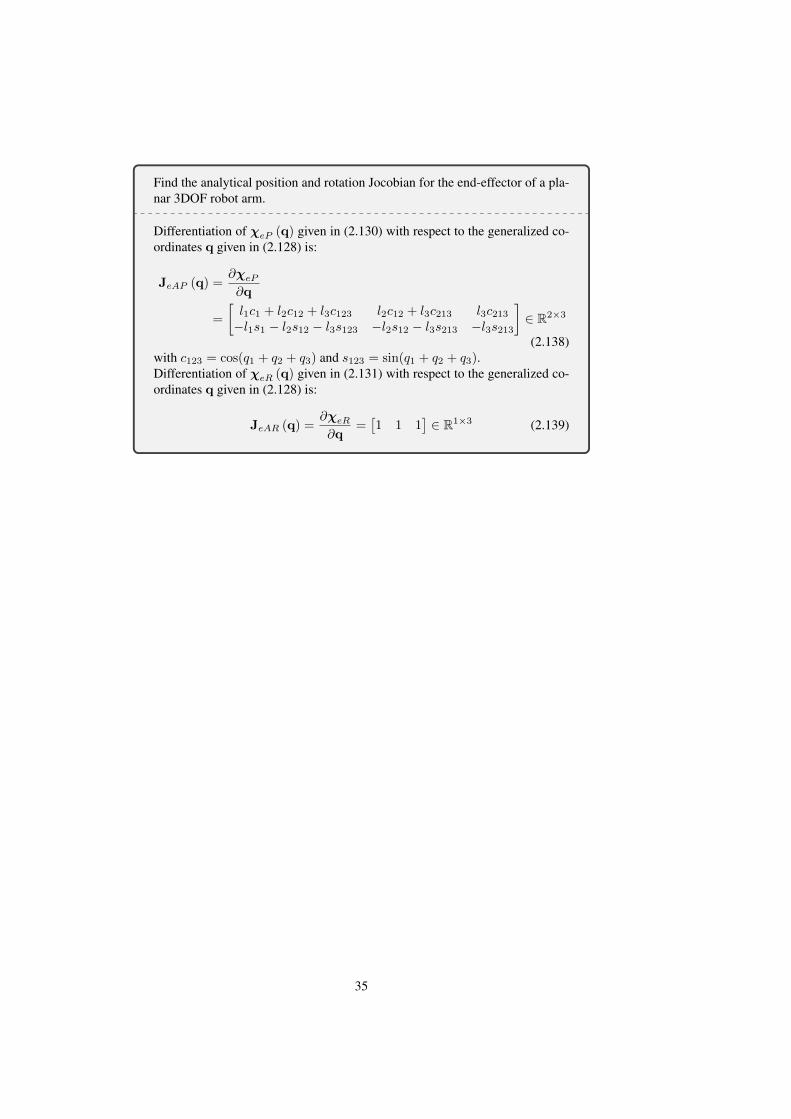
Find the analytical position and rotation Jocobian for the end-effector of a pla-nar 3DOF robot arm.

Differentiation of χeP (q) given in (2.130) with respect to the generalized co-ordinates q given in (2.128) is:

JeAP (q) =∂χeP∂q

=

[l1c1 + l2c12 + l3c123 l2c12 + l3c213 l3c213

−l1s1 − l2s12 − l3s123 −l2s12 − l3s213 −l3s213

]∈ R2×3

(2.138)with c123 = cos(q1 + q2 + q3) and s123 = sin(q1 + q2 + q3).Differentiation of χeR (q) given in (2.131) with respect to the generalized co-ordinates q given in (2.128) is:

JeAR (q) =∂χeR∂q

=[1 1 1

]∈ R1×3 (2.139)

35

e0x

e0z

e0y

eIz

eIx

eIye1x

e1y

e1z

e2y

e2x

e2z eEx

eEy

eEz

e(k−1)x

e(k−1)y

e(k−1)z

ekx

ekyekz

enx

enyenz

ωIk = Ωk

ωe = ΩE = ωIE

ve = rIE

ωI(k−1) = Ω(k−1)

rI(k−1)

rIk

r(k−1)k

Figure 2.13: Serial linkage arm with n moving links.

2.8.5 Geometric or Basic JacobianAs we have seen in (2.136), a Jacobian maps generalized velocities (in joint space)to time-derivatives of the end-effector configuration representation (which is not thelinear and angular velocity!). The associated partial differentiations of the end-effectorconfiguration JeA = ∂χe

∂q depends on the selected parameterization, especially on theparameterization of the rotation.

However, as we have learned previously, a body has a unique linear velocity veand angular velocity ωe. Hence, there must exist a unique Jacobian that relates thegeneralized velocity q to the velocity of the end-effector (linear ve and angular ωe):

we =

(veωe

)= Je0 (q) q. (2.140)

Je0 is called the geometric (or basic) Jacobian and it has in the most general cases thedimension 6×nj . Please also note at this point that the geometric Jacobian has a basisA as it maps generalized velocities to end-effector velocities represented in a specificcoordinate frame

Awe = AJe0 (q) q. (2.141)

Addition and Subtraction of Geometric Jacobians

From basic kinematics we know that the velocity of a point C can be calculated fromthe velocity of a point B and the relative velocity between B and C:

wC =

(vCωC

)= wB + wBC

JC q = JBq + JBC q

. (2.142)

36

From this we can identify that geometric Jacobians can be simply added

AJC = AJB + AJBC , (2.143)

as long as they are represented with respect to the same reference frame.

Calculation of geometric Jacobian using Rigid Body Formulation

From the analysis of the velocities of points on moving bodies (c.f. (2.110)) applied tothe serial linkage depicted in Fig. 2.13, it follows that the velocity of linkage k is givenby

rIk = rI(k−1) + ωI(k−1) × r(k−1)k. (2.144)

Please keep again in mind that for numerical addition it is crucial that all the vectorsare expressed in same coordinate system. When denoting the base frame as 0 and theend-effector frame as n+ 1, the end-effector velocity can be written as

rIE =

n∑

k=1

ωIk × rk(k+1). (2.145)

Using nk to represent the rotation axis of joint k such that

ω(k−1)k = nkqk (2.146)

and recalling thatωI(k) = ωI(k−1) + ω(k−1)k, (2.147)

the angular velocity of body k can be written as

ωIk =

k∑

i=1

niqi. (2.148)

Substituting this in (2.145) and rearranging terms results to

rIE =

n∑

k=1

(k∑

i=1

(niqi)× rk(k+1)

)(2.149)

=

n∑

k=1

nkqk ×n∑

i=k

ri(i+1) (2.150)

=

n∑

k=1

nkqk × rk(n+1) (2.151)

Bringing this in matrix formulation yields the geometric Jacobian

rIE =[n1 × r1(n+1) n2 × r2(n+1) . . . nn × rn(n+1)

]︸ ︷︷ ︸

Je0P

q1

q2

...qn

(2.152)

Given (2.148), the rotation Jacobian is

ωIE =

n∑

i=1

niqi =[n1 n2 . . . nn

]︸ ︷︷ ︸

Je0R

q1

q2

...qn

. (2.153)

37

Combining these two expressions yields the combined geometric Jacobian:

Je0 =

[Je0PJe0R

]=

[n1 × r1(n+1) n2 × r2(n+1) . . . nn × rn(n+1)

n1 n2 . . . nn

](2.154)

As stated at the beginning of this section, it is important that we need to define thisJacobian with respect to a basis, e.g. I (or any other frame):

IJe0 =

[IJe0PIJe0R

]=

[In1 × Ir1(n+1) In2 × Ir2(n+1) . . . Inn × Irn(n+1)

In1 In2 . . . Inn

].

(2.155)In this formulation, the rotation axis is given by

Ink = CI(k−1)(k−1)nk. (2.156)

Example 2.8.7: Basic Jacobian

ϕ1

ϕ2

ϕ3

e1x

e1ze2x

e2z e3x

e3z

eEx

eEz

l0

l1

l2

l3

ve

ωe

e0x = eIx

e0z = eIz

Determine the basic Jacobian for this planar robot arm

The generalized coordinates are

q =

q1

q2

q3

=

ϕ1

ϕ2

ϕ3

(2.157)

38

Step 1: determine the rotation matrices

CI1 =

c1 0 s1

0 1 0−s1 0 c1

(2.158)

CI2 = CI1 ·

c2 0 s2

0 1 0−s2 0 c2

=

c12 0 s12

0 1 0−s12 0 c12

(2.159)

CI3 = CI2 ·

c3 0 s3

0 1 0−s3 0 c3

=

c123 0 s123

0 1 0−s123 0 c123

, (2.160)

with s123 = sin (q1 + q2 + q3) and c123 = cos (q1 + q2 + q3) .Step 2: determine the local rotation axis (k−1)nk:

0n1 = 1n2 = 2n3 = ey (2.161)

Step 3: determine the rotation axis Ink = CI(k−1) · (k−1)nk:

In1 = 0n1 = ey (2.162)

In2 = CI1 · 1n2 = ey (2.163)

In3 = CI2 · 2n3 = ey (2.164)

Step 4: determine the position vectors from joint to end-effector:

Ir1E = Ir12 + Ir23 + Ir3E (2.165)= CI1 · 1r12 + CI2 · 2r23 + CI3 · 3r3E (2.166)

= l1

sq10cq1

+ l2

s12

0c12

+ l3

s123

0c123

(2.167)

Ir2E = Ir23 + Ir3E (2.168)= CI2 · 2r23 + CI3 · 3r3E (2.169)

= l2

s12

0c12

+ l3

s123

0c123

(2.170)

Ir3E = Ir3E (2.171)= CI3 · 3r3E (2.172)

= l3

s123

0c123

(2.173)

Step 5a: determine the position Jacobian:

IJe0P =[In1 × Ir1E In2 × Ir2E In3 × Ir3E

](2.174)

=

l1c1 + l2c12 + l3c123 l2c12 + l3c123 l3c123

0 0 0−l1s1 − l2s12 − l3c123 −l2s12 − l3s123 −l3s123

(2.175)

39

Step 5b: determine the rotation Jacobian:

IJe0R =[In1 In2 . . . Inn

](2.176)

=

0 0 01 1 10 0 0

(2.177)

2.8.6 Relation between Geometric and Analytic Jacobian MatrixAs introduced in section 2.2.1 and section 2.5.1, there exists a mapping between thedifferentials of the end-effector representation parameters χe and the twist we consist-ing of linear and angular velocities. This relationship also shows up in the mappingof the representation dependent Jacobians given by a partial differentiation of positionand rotation with respect to generalized coordinates JeA = ∂χe

∂q ∈ Rme×nj and thegeometric Jacobian Je0 ∈ R6×nj . Given that

χe = JeA (q) q with JeA (q) ∈ Rme×nj (2.178)

we = Je0 (q) q with Je0 (q) ∈ R6×nj (2.179)

χe = Ee (χe) we with Ee (χe) =

[EP 00 ER

]∈ Rme×6 (2.180)

the following mapping holds

JeA (q) = Ee (χ) Je0 (q) (2.181)

Please note that the parameterization dependent matrices E and E−1 were derivedearlier:

• Cartesian coordinates (2.12)

• Cylindrical coordinates (2.14) and (2.15)

• Spherical coordinates (2.16) and (2.17)

• Euler Angles

– XYZ: (2.77) and (2.78)

– ZYX: (2.75) and (2.76)

– ZYZ: (2.79) and (2.80)

• Quaternions (2.87) and (2.88)

• Angle Axis (2.91) and (2.92)

• Rotation Vector (2.95) and (2.96)

Literature often does not distinguish between geometric and analytic Jacobian.Mostly, when writing J it is referred to the geometric Jacobian. The same holds forthis course. For planar systems, the analytical and geometric Jacobian are identical.

40