NUMBER

749

JULY2015

Updated Ambient Concentrations of Toxic Chemicals in San Francisco Bay SedimentsJuly 2015

By:

Don Yee, Philip Trowbridge and Jennifer Sun

CLEAN WATER / RMP

S A N F R A N C I S C O E S T U A RY I N S T I T U T E 4911 Central Avenue, Richmond, CA 94804 • p: 510-746-7334 (SFEI) • f: 510-746-7300 • www.sfei.org

THIS REPORT SHOULD BE CITED AS:

Yee, D., Trowbridge, P., and Sun, J. 2015. Updated Ambient Concentrations of Toxic Chemicals in San Francisco Bay Sediments. San Francisco Estuary Institute, Richmond, CA. Contribution # 749. This work was supported by the Regional Monitoring Program for Water Quality in San Francisco Bay

Updated ambient concentrations of toxic chemicals in

San Francisco Bay sediments

July 24, 2015

Don Yee, Phil Trowbridge, and Jennifer Sun San Francisco Estuary Institute 4911 Central Avenue Richmond, CA 94604 www.sfei.org

2

Introduction Regulation of dredging and dredged material disposal or reuse under the San Francisco Bay Long Term Management Strategy for Dredging (LTMS) involves, in part, evaluation of sediment chemistry characteristics. For dredged material in California, for most chemicals, there are no numeric sediment quality standards or objectives that define chemical suitability for disposal or reuse at particular placement sites.1 Consequently, to evaluate potential pollution problems and regulate dredging, the San Francisco Bay Regional Water Quality Control Board (Regional Board) compares contaminant concentrations in Bay-dredged sediments to: (1) published contaminant screening values and other guidelines; (2) contaminant concentrations at reference sites; and (3) where available and appropriate, ambient sediment contaminant concentrations for the Bay as a whole. The first estimates of ambient sediment contaminant concentrations were made in 1998 by the Regional Board (SFBRWQCB, 1998). Since then, the ambient sediment concentrations have been updated in 2011, 2012, 2013, and 2014 for a only a small subset of high priority contaminants (mercury, polycyclic aromatic hydrocarbons [PAHs] and polychlorinated biphenyls [PCBs]). The calculations were not published in report but rather were posted on the website of the Regional Monitoring Program (RMP) for Water Quality in San Francisco Bay2. The purpose of this memo is to update the ambient sediment contaminant concentrations for all contaminants routinely monitored by the RMP, including nearly all contaminants with 1998 ambient sediment contaminant concentrations, using the most recent RMP sediment data (through 2012). In this report, the term “ambient sediment contaminant concentration” refers to a reference ambient condition for regulatory use that is different from the Bay-wide average sediment concentrations reported by the San Francisco Estuary Institute (SFEI) in the RMP “Pulse of the Estuary” reports. The term refers to the upper limits of typical sediment concentrations, not average values. The 1998 Ambient Sediment Values The Regional Board established the first set of ambient sediment contaminant concentrations in 1998 to fulfill a need for reference concentrations of toxic chemicals in Bay sediments that staff could use to evaluate potential pollution problems (SFBRWQCB, 1998). Since San Francisco Bay sediments are not totally free of anthropogenic and naturally occurring pollutants, the Regional Board defined “ambient” sediment concentrations as the typical range of 1 Pursuant to the Water Quality Control Plan for Enclosed Bays and Estuaries - Part 1 Sediment Quality, California’s Sediment Quality Objectives (SQOs) do not apply to dredged material suitability determinations. However, strict sediment chemistry limits may be established for individual contaminants or locations under Bay-wide TMDLs, site-specific remediation decisions, etc. 2 The results of the ambient sediment concentration calculations calculated since 2011 can be found on the RMP website: http://sfei.org/content/dredged-material-testing-thresholds-san-francisco-bay-area-sediments

3

concentrations one would expect to find in sediment in the less polluted, or “cleaner”, portions of the Bay. Contaminant concentrations above the threshold were considered elevated relative to the ambient population of sediment data. The Regional Board derived the 1998 ambient concentrations using RMP and Bay Protection and Toxic Cleanup Program fixed-station data collected from 1991-1995, setting the thresholds at the 95% upper tolerance limit of the 85th percentile concentrations (SFBRWQCB, 1998). Updated Ambient Sediment Values The original ambient sediment values from the 1998 analysis are now fairly old and are based on a relatively small data set compared to the amount of currently available sediment chemistry data from the RMP. In 2011, the LTMS agencies agreed upon a statistically robust definition of ambient Bay sediment contaminant concentrations that is relevant for dredged material regulatory use, while remaining based on data collected routinely by the RMP. Ambient sediment concentrations were defined as:

the 90% upper confidence limit of the 90th percentile concentrations using the most recent 10 years of data from the RMP’s randomized Bay-wide sediment sampling stations, after removal of statistical outliers due to highly contaminated samples (USACE/USEPA, 2011).

In 2011, SFEI and the LTMS agencies updated the ambient values for a small subset of sediment contaminants that are subject to total maximum daily load (TMDL) limits for in-Bay dredged material disposal (mercury and total PCBs) and/or bioaccumulation testing thresholds (mercury, total PCBs, total PAHs, total DDTs, total chlordane, dieldrin, and dioxins/furans). In subsequent years, the ambient values for mercury, total PCBs, and total PAHs have been updated with newer data and the latest results have been published on the RMP website2. This memo contains the latest update to the ambient sediment contaminant concentrations for not just the contaminants associated with TMDLs or bioaccumulation testing but also another 91 contaminants that have been routinely monitored in Bay sediments by the RMP. The ambient contaminant concentrations were calculated using the methodology outlined in USACE/USEPA (2011) using valid data from the most recent 10 years of the RMP’s randomized Bay-wide sediment sampling. For metals and other inorganic contaminants, data from 10 rounds of sediment sampling between 2003 and 2012 were used in the analysis. The analysis of organic contaminants was based on 8 rounds of sediment sampling from 2002, 2003, and 2007-20123. 3 Data for organic contaminants includes data collected and analyzed by the RMP during 2002-2003 and 2007-2012. Organic contaminant data collected and analyzed by the RMP in the 2004-2006 period have been excluded from the calculation due to an laboratory analytical artifact discovered in 2013 that resulted in underestimates of concentrations by 40% to 400% for a subset of samples later selected for reanalysis. Performance on quality control samples conducted with the initial analyses were within typical method acceptance limits (e.g., for EPA 1668 for PCBs). However, the QC samples were less impacted by the artifact (incomplete extraction due to moisture) for various reasons; certified reference materials typically are distributed pre-dried and homogenized, and matrix spikes

4

For dioxins/furans, the analysis is based on data from 2008-2010 because these contaminants were only measured as an RMP special study for this period. Data from historical fixed sampling stations that are not part of the RMP randomized sampling design were excluded. Outliers were removed to exclude any highly contaminated samples using an updated methodology described in Appendix A4. The RMP field sampling methodology includes visual selection of fine-grained sediments, and thus the ambient concentrations are representative of sediments with greater than 40% fines, which is typical of most sediments dredged in the Bay. Table 1 compares the Bay’s updated ambient sediment contaminant concentrations (2002-2012 data) to the original values from the SFBRWQCB (1998) report (1991-1995 data). Histograms illustrating the outliers and the ambient values for each of the contaminants are displayed in Appendix B. Ambient sediment concentrations (2002-2012) calculated as the 99th percentile 90% UTL are listed in Appendix C. Discussion The updated ambient sediment concentrations are generally lower than the values from the SFBRWQCB (1998) report but the changes vary by the type of contaminant. For metals, the updated ambient concentrations are 0.3-46% lower than the SFBRWQCB (1998) values. The updated ambient concentrations for individual pesticides are 33-94% lower than the previous values. Total PCB concentrations (total of 40 congeners) are 15% lower. The one exception to this pattern is PAHs. Changes in the ambient concentrations of individual PAHs are mixed, but ambient concentrations of total PAHs (total of 25 contaminants listed in Table 1) are 34% higher than the values in the SFBRWQCB (1998) report. This analysis of change was not possible for a number of contaminants because ambient concentrations were not calculated in 1998. The observed changes in the ambient sediment contaminant concentrations between this memo and the SFBRWQCB (1998) report likely have many explanations. First, the sampling design has changed from a fixed-station design in 1991-1995 to a randomized design in 2002-2012. Second, the algorithm used to calculate the ambient concentrations has changed and an automated method for identifying and excluding outliers has been added. Finally, the changes may reflect actual trends in the environment such as a spike of PAH concentrations in the Bay following the Cosco Busan oil spill in 2007 (SFEI, 2013). Ambient sediment concentrations can be used by the LTMS agencies in a variety of ways, including as a basis for considering updates to guidelines for beneficial reuse of dredged material at wetland restoration project sites near the margins of the Bay. However, it is important to note are typically added only shortly before analysis and thus not deeply embedded in the matrix where moisture would more impact extraction. Exclusion of this data has only had a moderate impact on the estimate of the 2014 ambient concentrations (based on 2002-2003 and 2007-2012 data, a 90th percentile 90% UTL of 18.3 ug/kg dw for total PCBs shown in Table 1) compared to the 2013 ambient values (based on 2002-2011 data, a 90th percentile 90% UTL of 17.4 ug/kg dw). 4 The description provided in Appendix A is also available at the following link: http://sfei.org/content/dredged-material-testing-thresholds-san-francisco-bay-area-sediments

5

that even if contaminant concentrations in a dredged material project are below the upper bound calculations of ambient sediment concentrations, this alone does not indicate that the dredged material is suitable for placement at any particular site. Ambient levels may be higher than environmentally desirable for some placement sites, while at other sites ambient concentrations may be far below levels of concern that need to be regulated. Ambient concentrations by themselves are not sediment screening values, and should not be used to make regulatory decisions. However, understanding how potential regulatory goals or limits under consideration may relate to existing Bay ambient sediment concentrations can be important in informing regulatory decisions that are both effective and feasible to implement. Recommendations The methodology for calculating ambient sediment contaminant concentrations calls for using the most recent 10 years of data (USACE/USEPA, 2011). However, starting in 2014, the RMP reduced the frequency of open Bay sediment sampling to once every 4 years. The result is that a 10-year time window will only include 3 sampling rounds with the new RMP sampling schedule. The calculated ambient concentrations will be based on less data and might be less stable. For comparison, the values in this report are based on 8-10 rounds of sediment sampling. To address this potential problem, the LTMS agencies may wish to consider a change to the calculation methodology. At a minimum, it is recommended that the time window for data be increased to 13 years, which would allow for 4 sets of data in each calculation. Another option is to specify a minimum number of data sets and an upper limit time window required in order to run the calculation of an ambient sediment concentration for a particular contaminant (e.g., 4 datasets less than 15 years old). The latter approach would be helpful for determining which contaminants will have enough data to calculate updated values since the target parameters for RMP sampling sometimes change. Further, the frequency of updates to the ambient sediment contaminant concentrations should match the frequency of RMP open Bay sediment sampling. It is recommended that the ambient sediment contaminant concentrations for mercury, PCBs, and PAHs be recalculated after each new round of RMP sediment sampling. For the longer list of contaminants, updates should occur after every other sampling round or every 8 years. References San Francisco Bay Regional Water Quality Control Board. 1998. Staff Report: Ambient Concentrations of Toxic Chemicals in San Francisco Bay Sediments. San Francisco Bay Regional Water Quality Control Board, Oakland, CA. http://www.swrcb.ca.gov/sanfranciscobay/publications_forms/documents/sfbaysediment.pdf

6

San Francisco Estuary Institute. 2013. The Pulse of the Bay: Contaminants of Emerging Concern. SFEI Contribution 701. San Francisco Estuary Institute, Richmond, CA. http://www.sfei.org/sites/default/files/Pulse%202013%20CECs(1).pdf U.S. Army Corps of Engineers and U.S. Environmental Protection Agency, Region 9. 2011. Memo to Robert S. Hoffmann, National Marine Fisheries Service, Long Beach, CA. http://www.sfei.org/sites/default/files/LTMS%20EFH%20full%20signed%20agreement%20FINAL%206-9-2011.pdf

7

Table 1. Ambient contaminant concentrations in San Francisco Bay area sediments.

Contaminant Ambient Sediment Values from SFBRWQCB (1998)2

(85th Percentile 95% UTL4)

Updated Ambient Sediment Values from this report3

(90th Percentile 90% UTL4)

METALS (mg/kw dw) 1991-1995 2003-2012 Arsenic 15.3 13.9

Cadmium 0.33 0.33 Chromium1 112 NA

Copper 68.1 53.9 Lead 43.2 25.1

Mercury 0.43 0.33 Nickel 112 98.3

Selenium 0.64 0.36 Silver 0.58 0.32

Zinc 158 136 PESTICIDES (ug/kg dw) 1991-1995 2002-2003, 2007-2012

Aldrin NA 0.03 Total Chlordane 1.1 0.34

Dieldrin 0.44 0.16 Endrin NA 0.01

Total DDT (total of 6 isomers) 7 4.68 DDD(o,p') NA 0.51 DDD(p,p') NA 1.98 DDE(o,p') NA 0.11 DDE(p,p') NA 1.98 DDT(o,p') NA 0.04 DDT(p,p') NA 0.27

Total HCH 0.78 0.05 Hexachlorobenzene 0.48 0.20

PAH (ug/kg dw) 1991-1995 2002-2003, 2007-2012 Total PAH 3390 4540

Total HPAH 3060 3870 Total LPAH 434 574

Acenaphthene 26.6 13.5 Acenaphthylene 31.7 32.6

Anthracene 88 80.1 Benz(a)anthracene 244 212

8

Contaminant Ambient Sediment Values from SFBRWQCB (1998)2

(85th Percentile 95% UTL4)

Updated Ambient Sediment Values from this report3

(90th Percentile 90% UTL4)

Benzo(a)pyrene 412 428 Benzo(b)fluoranthene 371 227

Benzo(e)pyrene 294 244 Benzo(g,h,i)perylene 310 416

Benzo(k)fluoranthene 258 231 Biphenyl 12.9 11.7 Chrysene 289 252

Dibenz(a,h)anthracene 32.7 49.9 Dibenzothiophene NA 16.3

Dimethylnaphthalene, 2,6- 12.1 13 Fluoranthene 514 620

Fluorene 25.3 27.1 Indeno(1,2,3-c,d)pyrene 382 337

Methylnaphthalene, 1- 12.1 13.4 Methylnaphthalene, 2- 19.4 20.8

Methylphenanthrene, 1- 31.7 37.6 Naphthalene 55.8 56.4

Perylene 145 216 Phenanthrene 237 176

Pyrene 665 791 Trimethylnaphthalene, 2,3,5- 9.8 7.43

PCB (ug/kg dw) 1991-1995 2002-2003, 2007-2012 Total PCB (sum of 40 congeners) 21.6 18.3

PCB 8 NA 0.14 PCB 18 NA 0.07 PCB 28 NA 0.28 PCB 31 NA 0.13 PCB 33 NA 0.08 PCB 44 NA 0.33 PCB 49 NA 0.25 PCB 52 NA 0.39 PCB 56 NA 0.14 PCB 60 NA 0.07 PCB 66 NA 0.48 PCB 70 NA 0.59

9

Contaminant Ambient Sediment Values from SFBRWQCB (1998)2

(85th Percentile 95% UTL4)

Updated Ambient Sediment Values from this report3

(90th Percentile 90% UTL4)

PCB 87 NA 0.46 PCB 95 NA 0.60 PCB 99 NA 0.65

PCB 101 NA 1.15 PCB 105 NA 0.36 PCB 110 NA 1.04 PCB 118 NA 0.98 PCB 128 NA 0.28 PCB 132 NA 0.37 PCB 138 NA 1.83 PCB 141 NA 0.20 PCB 149 NA 1.25 PCB 151 NA 0.56 PCB 153 NA 1.74 PCB 156 NA 0.16 PCB 158 NA 0.15 PCB 170 NA 0.47 PCB 174 NA 0.49 PCB 177 NA 0.36 PCB 180 NA 1.02 PCB 183 NA 0.37 PCB 187 NA 0.87 PCB 194 NA 0.33 PCB 195 NA 0.11 PCB 201 NA 0.05 PCB 203 NA 0.17

PBDE (ug/kg dw) 1991-1995 2002-2003, 2007-2012 Total PBDE NA 5.47

DIOXIN (ng TEQ/kg dw) 1991-1995 2008-2010 Sum of Dioxins TEQ NA 1.83 Sum of Furans TEQ NA 1.07

1RMP stopped monitoring chromium in 2002. 2NA = Data Not Available 3The time period over which data was used to calculate the 2014 ambient sediment values are shown in the contaminant category titles. 4UTL = upper tolerance limit

10

Appendix A

Updated Outlier Detection Method Summary The report from USACE/USEPA (2011) contained an automated outlier detection method (see Attachment 3 of that report). This appendix describes the modifications that have been made to methodology from USACE/USEPA (2011) to make the statistical methods more robust. Background Using the original coding of the R script for identifying outliers, the addition of RMP PCB data from 2011 to the previous data set (2002-2010) resulted in a statistical artifact that caused a large percentage of the data (~11%) to be regarded as outliers; previous years’ analyses considered most of these same points not outliers (1% or less of the data were outliers). This issue arose due to a randomly occurring tight cluster of values in one portion of the distribution. The original outlier function used a moderately small percentage of the total data set (2.5%, with a minimum of 12 values) to determine a local average difference expected between points. This very tight cluster of values resulted in a gap to the next higher value (between 15.9 and 16.7 ppb) that had previously been considered unremarkable (<10x the local average difference) to be labeled as the gap to a set of outliers when the 2011 data were included. Modifications to the Outlier Detection Method in USACE/USEPA (2011) To prevent future flagging of such chance statistical anomalies as outlier gaps, the following modifications to the outlier auto-detection function have been made:

1. A larger percentage of the nearest lower values (5% of the total data) are used to calculate a local average difference. Increasing from 2.5 % to 5% of the population decreases the influence of any small cluster of tightly spaced points (the anomaly seen in the 2002-2011 data set). However, in the upper tail of the data distribution where we usually expect sparser spacing, using a larger percentage of the population decreases the apparent local difference by averaging in some more tightly spaced points in the main body of the distribution, potentially flagging more gaps. This change stabilizes the local average difference, decreasing the probability of finding gaps in the main body of the distribution, but increasing the likelihood in sparse areas of the upper tail.

2. Any outlier has to be at least 25% greater than the mean of its nearest lower neighbors (a running average 10% of the total data) to be considered “meaningful.” In many laboratory chemical analyses, a 25% difference in replicate measurements is acceptable, so the difference between a possible outlier and its nearest lower neighbors should be at least as large to account for measurement uncertainty. The difference to a running average of nearest lower neighbors rather than a single nearest lower neighbor is used, as otherwise a few values between low and high

11

concentration groups could bridge apparent gaps, causing no outliers to be found. The use of 10% of the data for the running average further ensures that a small set of sparse values cannot bridge the zone between low and high concentration groups.

3. Since our concern is about high outlier values, any outlier has to occur above the upper quartile value. This avoids a case where a minority of very low values (e.g., clean sites near Golden Gate) would create an apparent gap to the main population of results, causing all of the latter to be called outliers. Using the upper quartile as the threshold, a bimodal distribution, in which a slight majority of the data is in the lower group, would still result in the upper portion labeled as outliers.

Imposing all three of the modifications described above makes the detection of outlier groups more stable and resistant to chance anomalies in the data distribution. The current data set now includes 10 years of data, and future calculations using the USAOC/USEPA ambient sediment calculation method will only include the most recent 10 years of data. Existing outlier groups are therefore unlikely to change just by the filling in of gaps using new data with similar concentration distributions; only larger and real shifts in distribution (e.g., 5% or more of the total data bridging the gaps) will cause appreciable shifts in the subset of points being identified as outliers.

12

Appendix B

Histograms of RMP Sediment Data

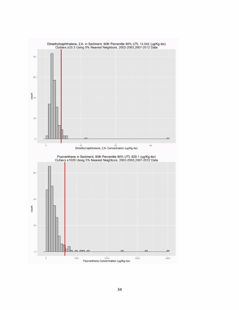
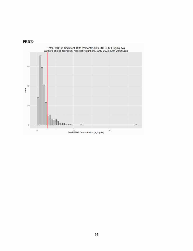
The RMP sediment data used to update the ambient sediment contaminant concentrations are shown on the following histogram plots. On each plot, the histogram shows the distribution of all RMP sediment data from randomized stations, the red line indicates the 90% upper tolerance limit of the 90th percentile concentration, and the title contains the concentration above which results were considered outliers. The years of data used in the analysis are also listed in the title to each plot.

13

Trace Metals

14

15

16

17

18

Pesticides

19

20

21

22

23

24

25

PAHs

26

27

28

29

30

31

32

33

34

35

36

37

38

39

40

PCBs

41

42

43

44

45

46

47

48

49

50

51

52

53

54

55

56

57

58

59

60

61

PBDEs

62

Dioxin TEQs

63

Appendix C

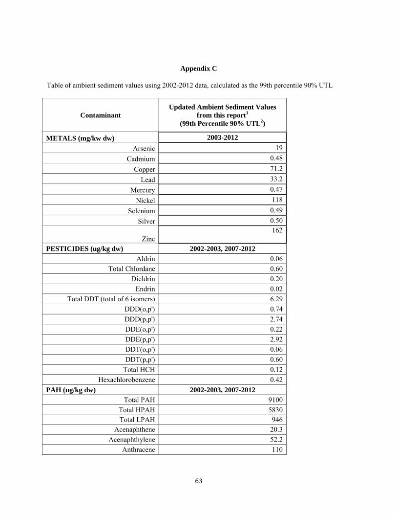
Table of ambient sediment values using 2002-2012 data, calculated as the 99th percentile 90% UTL

Contaminant Updated Ambient Sediment Values

from this report1 (99th Percentile 90% UTL2)

METALS (mg/kw dw) 2003-2012 Arsenic 19

Cadmium 0.48 Copper 71.2

Lead 33.2 Mercury 0.47

Nickel 118 Selenium 0.49

Silver 0.50

Zinc 162

PESTICIDES (ug/kg dw) 2002-2003, 2007-2012

Aldrin 0.06 Total Chlordane 0.60

Dieldrin 0.20 Endrin 0.02

Total DDT (total of 6 isomers) 6.29 DDD(o,p') 0.74 DDD(p,p') 2.74 DDE(o,p') 0.22 DDE(p,p') 2.92 DDT(o,p') 0.06 DDT(p,p') 0.60

Total HCH 0.12 Hexachlorobenzene 0.42

PAH (ug/kg dw) 2002-2003, 2007-2012 Total PAH 9100

Total HPAH 5830 Total LPAH 946

Acenaphthene 20.3 Acenaphthylene 52.2

Anthracene 110

64

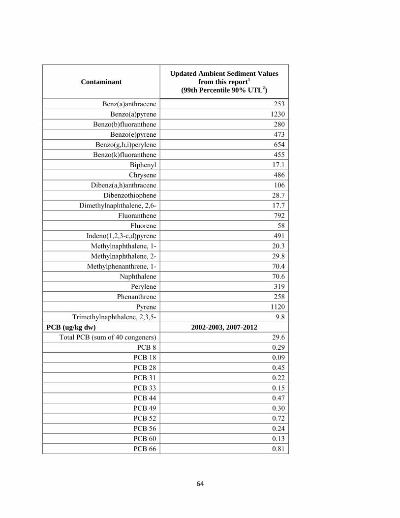
Contaminant Updated Ambient Sediment Values

from this report1 (99th Percentile 90% UTL2)

Benz(a)anthracene 253 Benzo(a)pyrene 1230

Benzo(b)fluoranthene 280 Benzo(e)pyrene 473

Benzo(g,h,i)perylene 654 Benzo(k)fluoranthene 455

Biphenyl 17.1 Chrysene 486

Dibenz(a,h)anthracene 106 Dibenzothiophene 28.7

Dimethylnaphthalene, 2,6- 17.7 Fluoranthene 792

Fluorene 58 Indeno(1,2,3-c,d)pyrene 491

Methylnaphthalene, 1- 20.3 Methylnaphthalene, 2- 29.8

Methylphenanthrene, 1- 70.4 Naphthalene 70.6

Perylene 319 Phenanthrene 258

Pyrene 1120 Trimethylnaphthalene, 2,3,5- 9.8

PCB (ug/kg dw) 2002-2003, 2007-2012 Total PCB (sum of 40 congeners) 29.6

PCB 8 0.29 PCB 18 0.09 PCB 28 0.45 PCB 31 0.22 PCB 33 0.15 PCB 44 0.47 PCB 49 0.30 PCB 52 0.72 PCB 56 0.24 PCB 60 0.13 PCB 66 0.81

65

Contaminant Updated Ambient Sediment Values

from this report1 (99th Percentile 90% UTL2)

PCB 70 0.95 PCB 87 0.60 PCB 95 1.28 PCB 99 1.25

PCB 101 2.26 PCB 105 0.49 PCB 110 1.93 PCB 118 1.33 PCB 128 0.51 PCB 132 0.44 PCB 138 2.62 PCB 141 0.31 PCB 149 2.56 PCB 151 1.29 PCB 153 2.63 PCB 156 0.22 PCB 158 0.30 PCB 170 0.66 PCB 174 0.70 PCB 177 0.53 PCB 180 2.18 PCB 183 0.48 PCB 187 1.11 PCB 194 0.41 PCB 195 0.14 PCB 201 0.12 PCB 203 0.23

PBDE (ug/kg dw) 2002-2003, 2007-2012 Total PBDE 21.4

DIOXIN (ng TEQ/kg dw) 2008-2010 Sum of Dioxins TEQ 2.69 Sum of Furans TEQ 1.35

1The time period over which data was used to calculate the ambient sediment values are shown in the contaminant category titles. 2UTL = upper tolerance limit