for and

PhD candidate:

Advisors:

Nil Garcia

Dr. Alexander M. Haimovich

Dr. Martial Coulon

April 29, 2015

Resources Allocation for Active Localization

◦ Summary

High Precision Passive Localization

◦ Introduction and context

◦ Problem statement and signal model

◦ Proposed approach

◦ Numerical results

Summary

Transmitters illuminate

target(s).

Application example: MIMO

radar

Source(s) emit their own

signals

Application example:

localization of mobile

equipment in cellular networks

Active Localization Passive Localization

Widely distributed transmitters and receivers

Transmitters access the medium using disjoint bandwidths of the spectrum.

CRLB on the target positions which depends on…

◦ Transmitter’s power

◦ Bandwidth of the signals

𝑠1 𝑠2 𝑠3

freq.

Total bandwidth

Rx

Tx

Tx

Target

Rx

Tx

Tx

Target

TOA-based

localization,

(multilateration)

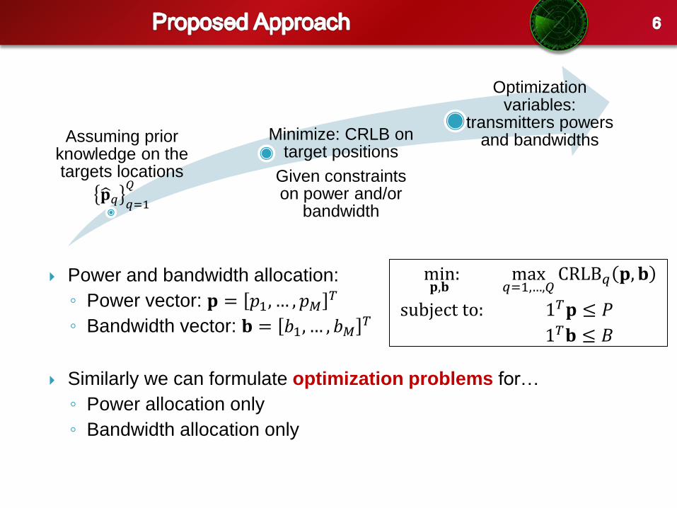
Power and bandwidth allocation:

◦ Power vector: 𝐩 = 𝑝1, … , 𝑝𝑀𝑇

◦ Bandwidth vector: 𝐛 = 𝑏1, … , 𝑏𝑀𝑇

Similarly we can formulate optimization problems for…

◦ Power allocation only

◦ Bandwidth allocation only

Assuming prior knowledge on the targets locations

𝐩 𝑞 𝑞=1𝑄

Minimize: CRLB on target positions

Given constraints on power and/or

bandwidth

Optimization variables:

transmitters powers and bandwidths

min𝐩,𝐛: max

𝑞=1,…,𝑄CRLB𝑞 𝐩, 𝐛

subject to: 1𝑇𝐩 ≤ 𝑃

1𝑇𝐛 ≤ 𝐵

CRLB𝑞 𝐩, 𝐛 not convex convex optimization methods

Sequential convex approximation

1. Convex approximation of the problem

2. Uses the solution for the next convex approximation

3. Stops upon practical convergence

Solve

convexified

problem

Solution at iteration 𝑛

𝐩 𝑛 , 𝐛 𝑛

Initialization

𝐩 0 , 𝐛 0

Stop at practical

convergence

𝐩 𝑛 , 𝐛 𝑛

= 𝐩 𝑛−1 , 𝐛 𝑛−1

With 5 transmitters, 10%, 50% and 70% reduction in localization error

in power, bandwidth and joint power-bandwidth allocating, respectively,

compared to uniform allocation.

Goal: Localization (geolocation) of RF emitters in multipath

environments

Challenges:

◦ Line-of-sight (LOS) paths

◦ Non-line-of-sight (NLOS) paths

◦ Blocked LOS paths (e.g. indoor)

Applications:

◦ Indoor positioning

◦ Defense/first responders

◦ Location based services

◦ E911

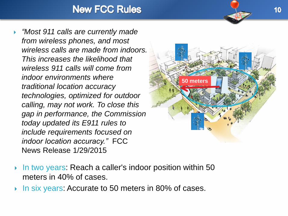
“Most 911 calls are currently made

from wireless phones, and most

wireless calls are made from indoors.

This increases the likelihood that

wireless 911 calls will come from

indoor environments where

traditional location accuracy

technologies, optimized for outdoor

calling, may not work. To close this

gap in performance, the Commission

today updated its E911 rules to

include requirements focused on

indoor location accuracy.” FCC

News Release 1/29/2015

50 meters

In two years: Reach a caller's indoor position within 50

meters in 40% of cases.

In six years: Accurate to 50 meters in 80% of cases.

Relies on TOA’s

The eNodeB assists the UE so it

can synchronize with the GNSS

signals faster.

Not more accurate than GNSS

Challenged in dense urban and

indoor situations

Relies on TOA/TDOA or signal

strength

Does not require GPS

Requires synchronization among

base stations.

Requires signals from at least 3

eNodeB

Challenged in dense urban and

indoor situations

Assisted Global Navigation

Satellite System (A-GNSS)

Positioning

Advanced Forward Link

Trilateration (AFLT)/TDOA

Satellite

eNodeB

Positioning signal

Assisting information

Connection needed to only a

signle eNodeB

Very coarse accuracy

Relies on TDOA’s

Uses uplink signals

Computation done in the

eNodeB’s instead of the UE.

Requires synchronization among

eNodeB’s

Challenged in dense urban and

indoor situations

Cell-ID-based Positioning Uplink TDOA (RAN)

Cell

eNodeB

Positioning signal

Methods designed for open outdoor spaces do not work well in

congested urban areas and indoors.

Source: Nextnav 2012

Emerging technology of Cloud Radio Access Network (Cloud-RAN or C-

RAN) shifts processing and complexity to the cloud thus simplifying the

design of sensors.

Concept of relatively simple sensors linked to the cloud may be ported to

applications other than cellular, for example first responders.

Optic fiber

Cloud computing

Localization over multipath channels still an open problem!

Goal

Estimate sources’ locations

Assumptions

Network of distributed sensors with fixed, known locations

Sensors have ideal communication with fusion center

Emitters’ waveforms and their timing are known

Synchronization

◦ Time synchronization between sensors and emitters

◦ No phase synchronization

Observation time << channel coherence time

Time-invariant multipath channel

No prior information on multipath channel

Fusion

center

Signal at the 𝑙-th sensor:

𝑦𝑙 𝑛 = 𝛼𝑙𝑞𝑠𝑞 𝑛 − 𝜏𝑙 𝐩𝑞

𝑄

𝑞=1

+ 𝛼𝑙𝑞(𝑚)𝑠𝑞 𝑛 − 𝜏𝑙𝑞

(𝑚)

𝑀𝑙𝑞

𝑚=1

𝑄

𝑞=1

+ 𝑛𝑙(𝑡)

𝑄 emitters and 𝐿 sensors

𝑠𝑞(𝑡): the signal of the 𝑞-th emitter

LOS parameters:

𝛼𝑙𝑞: complex amplitude of the LOS path between emitter q and sensor 𝑙

𝜏𝑙 𝐩𝑞 : propagation time from location 𝐩𝑞 to sensor 𝑙

NLOS parameters

𝛼𝑙𝑞(𝑚): complex amplitude of the 𝑚-th NLOS path between emitter

q and sensor 𝑙

𝜏𝑙𝑞(𝑚)

: propagation time of 𝑚-th NLOS path from between emitter q

and sensor 𝑙

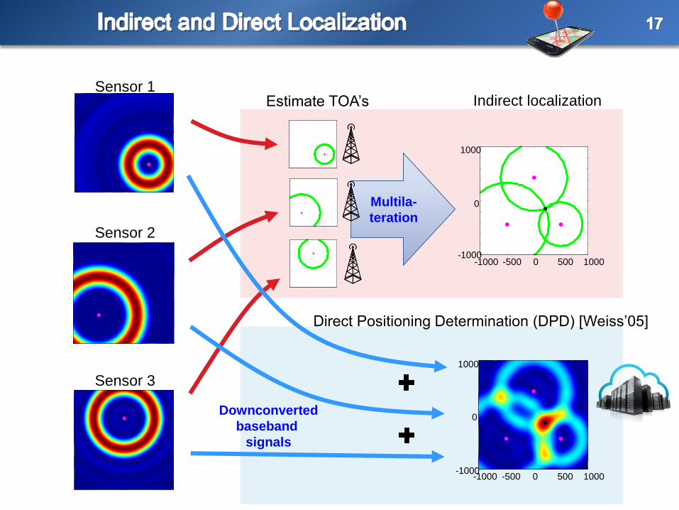
Sensor 1

-1000 -500 0 500 1000 -1000

0

1000

-1000 -500 0 500 1000 -1000

0

1000

Multila-

teration

Sensor 2

Sensor 3

Indirect localization

Direct Positioning Determination (DPD) [Weiss’05]

Downconverted

baseband

signals

Estimate TOA’s

Direct positioning determination

(DPD) is asymptotically optimal in the

maximum likelihood sense for ideal

LOS channels

DPD performs better than

multilateration at low SNR

DPD does not address localization in

multipath:

◦ Non-line-of-sight (NLOS) paths

◦ Blocked LOS paths

Various metrics were

suggested

NLOS signals bounce

only once

Known number of

reflectors

Joint estimation of

reflectors and emitters

locations.

Works only for discrete

MP contributions

If LOS is blocked

error

time

Mitigate/reject

contribution from

sensors with strong

NLOS [Chen’99]

Measure TOA of 1st

arrival [Lee’02]

Single-bounce

geometric model

[Liberti,Rappaport’96]

ML estimation in white Gaussian noise

◦ Measurements

◦ Unknown parameters related to LOS paths

◦ Unknown parameters related to NLOS paths

min𝐩1,…,𝐩𝑄𝛼11,…,𝛼𝐿𝑄𝑀11,…,𝑀𝐿𝑄

𝜏11(1),…,𝜏𝐿𝑄(𝑀𝐿𝑄)

𝑏111 ,…,𝑏𝐿𝑄

𝑀𝐿𝑄

𝑦𝑙 𝑛 − 𝛼𝑙𝑞𝑠𝑞 𝑛 − 𝜏𝑙 𝐩𝑞

𝑄

𝑞=1

− 𝛼𝑙𝑞(𝑚)𝑠𝑞 𝑛 − 𝜏𝑙𝑞

(𝑚)

𝑀𝑙𝑞

𝑚=1

𝑄

𝑞=1

2𝑁

𝑛=1

𝐿

𝑙=1

Large unknown parameters pool

Infeasible complexity

Overfitted solution even if problem could be solved

Procedure

Key info

Goal

Deconvolution

Multipath mitigation

LOS path is first arrival

MP paths are sparse

Estimate TOA’s : 𝜏 1 < 𝜏 2… < 𝜏 𝑇

and their amplitudes

𝑎 1, 𝑎 2, … , 𝑎 𝑇

at each sensor.

Exploit sparsity

Remove 2nd and later

estimated arrivals from

signals

𝑟 𝑙 𝑡 = 𝑟𝑙 𝑡 − 𝑎 𝑖𝑠(𝑡 − 𝜏 𝑖)𝑇

𝑖=1

Localization

Estimate sources locations

Sources are sparse

LOS paths originate from

common location

Multipath is local

Direct approach relies

directly on observations

Cloud-based

Formulate and solve a

convex optimization

problem

Least number of sources

and NLOS that describe

the measured signals

MP mitigation

(1) Sparse number of arrivals

(2) At each sensor, estimate propagation delays of MP paths

(3) Subtract out from data

For sensor 𝑙, propagation delays are solution to problem

min𝐱… 𝐲𝑙 − 𝐀𝐱

2+ 𝜆 𝐱 1

Here, the 𝑁 × 𝐷𝑄 matrix 𝐀 is a dictionary of the received signals for

all possible delay discrete MP delays and waveforms:

𝐀 = 𝐬1(0) ⋯ 𝐬1 𝐷 − 1 𝜏𝑟𝑒𝑠

.….𝐬𝑄(0) ⋯ 𝐬𝑄 𝐷 − 1 𝜏𝑟𝑒𝑠

Lasso optimization problem

◦ Solved by convex optimization methods.

◦ Yields sparsest solution. ≈ ×

All measurements are contained in a single matrix of size 𝑁 × 𝐿:

𝐑 =𝑦1(0) … 𝑦𝐿(0)⋮ ⋱ ⋮

𝑦1(𝑁 − 1) … 𝑦1(𝑁 − 1)

= 𝛼1𝑞𝐬𝑞 𝜏1 𝐩𝑞 ⋯ 𝛼𝐿𝑞𝐬𝑞 𝜏𝐿 𝐩𝑞

𝑄

𝑞=1

+ ⋯ 0 𝛼𝑙𝑞(𝑚)𝐬𝑞 𝜏𝑞𝑙

(𝑚)0 ⋯

𝑀𝑞𝑙

𝑚=1

𝐿

𝑙=1

𝑄

𝑞=1

+𝐖

𝐬𝑞(𝜏) stacks 𝑁 times samples of the emitted signal delayed by 𝜏:

𝐬𝑞(𝜏) = 𝑠𝑞 0 − 𝜏 ⋯ 𝑠𝑞 𝑁 − 1 𝑇 − 𝜏𝑇

Sensors

Samples

Observations at all sensors: 𝐑

Find sparsest number of sources and NLOS paths that

explains the observations Recover the source’s location

𝐑 = 𝛼1𝑞𝐬𝑞 𝜏1 𝐩𝑞 ⋯ 𝛼𝐿𝑞𝐬𝑞 𝜏𝐿 𝐩𝑞

𝑄

𝑞=1

+ ⋯ 0 𝛼𝑙𝑞(𝑚)𝐬𝑞 𝜏𝑞𝑙

(𝑚)0 ⋯

𝑀𝑞𝑙

𝑚=1

𝐿

𝑙=1

𝑄

𝑞=1

How to decide on the number of NLOS paths 𝑀𝑞𝑙 and estimate the

sources’ location? Apply tools from compressive sensing

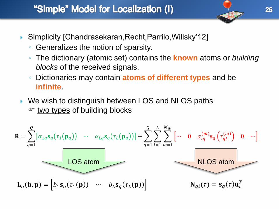
Simplicity [Chandrasekaran,Recht,Parrilo,Willsky’12]

◦ Generalizes the notion of sparsity.

◦ The dictionary (atomic set) contains the known atoms or building

blocks of the received signals.

◦ Dictionaries may contain atoms of different types and be

infinite.

We wish to distinguish between LOS and NLOS paths

two types of building blocks

𝐑 = 𝛼1𝑞𝐬𝑞 𝜏1 𝐩𝑞 ⋯ 𝛼𝐿𝑞𝐬𝑞 𝜏𝐿 𝐩𝑞

𝑄

𝑞=1

+ ⋯ 0 𝛼𝑙𝑞(𝑚)𝐬𝑞 𝜏𝑞𝑙

(𝑚)0 ⋯

𝑀𝑞𝑙

𝑚=1

𝐿

𝑙=1

𝑄

𝑞=1

LOS atom NLOS atom

𝐋𝑞 𝐛, 𝐩 =.

𝑏1𝐬𝑞 𝜏1 𝐩 ⋯ 𝑏𝐿𝐬𝑞 𝜏𝐿 𝐩 𝐍𝑞𝑙(𝜏) = 𝐬𝑞 𝜏 𝐮𝑙𝑇

Simple model of the data is

𝐑 = 𝑐𝑘𝐀𝑘

𝐾

𝑘=1

…where the atoms 𝐀𝑘 belong to the dictionary 𝒜

𝐀𝑘 ∈ 𝒜 = 𝒜𝐿𝑂𝑆 ⋃𝒜𝑁𝐿𝑂𝑆,

composed of LOS atoms…

𝒜𝐿𝑂𝑆 = 𝐋𝑞 𝐛, 𝐩 : 𝐛 ∈ ℂ𝐿, 𝐩 ∈ 𝑆

𝑄

𝑞=1

…and NLOS atoms:

𝒜𝑁𝐿𝑂𝑆 = 𝐍𝑞𝑙 𝜏 : 𝜏 ∈ 0, 𝜏𝑚𝑎𝑥

𝐿

𝑙=1

𝑄

𝑞=1

𝑆

Finding the simplest explanation (smallest linear combination of

atoms) of the data is an NP-hard problem.

The atomic norm ⋅ 𝒜 is the ℓ1-norm ⋅ 1 when 𝒜 is the set of

unit-norm one-sparse vectors.

𝐑 𝒜= min. 𝑐𝑘𝑘 such that 𝐑 = 𝑐𝑘𝐀𝑘𝑘

Simplicity is induced by minimizing the atomic norm:

The received signals are assumed simple in the sense that they

can expressed by a relatively small number of atoms

Approximate explanation

in presence of noise

Induces low number of atoms min𝑐𝑘. 𝑐𝑘

𝑘

subject to: 𝐑 − 𝑐𝑘𝐀𝑘𝑘 2

≤ 𝜖

min𝑐𝑘. 𝑐𝑘

𝑘

subject to: 𝐑 − 𝑐𝑘𝐀𝑘𝑘 2

≤ 𝜖

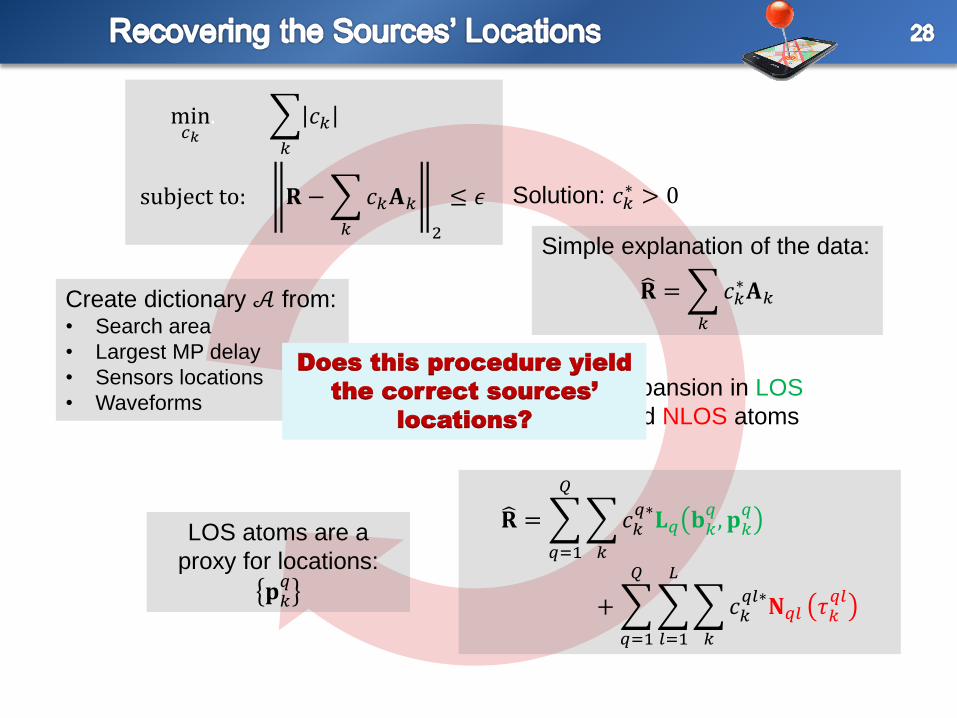
Simple explanation of the data:

𝐑 = 𝑐𝑘∗𝐀𝑘

𝑘

𝐑 = 𝑐𝑘𝑞∗𝐋𝑞 𝐛𝑘

𝑞, 𝐩𝑘𝑞

𝑘

𝑄

𝑞=1

+ 𝑐𝑘𝑞𝑙∗𝐍𝑞𝑙 𝜏𝑘

𝑞𝑙

𝑘

𝐿

𝑙=1

𝑄

𝑞=1

Solution: 𝑐𝑘∗ > 0

Expansion in LOS

and NLOS atoms

LOS atoms are a

proxy for locations:

𝐩𝑘𝑞

Create dictionary 𝒜 from: • Search area

• Largest MP delay

• Sensors locations

• Waveforms

Does this procedure yield

the correct sources’

locations?

Example:

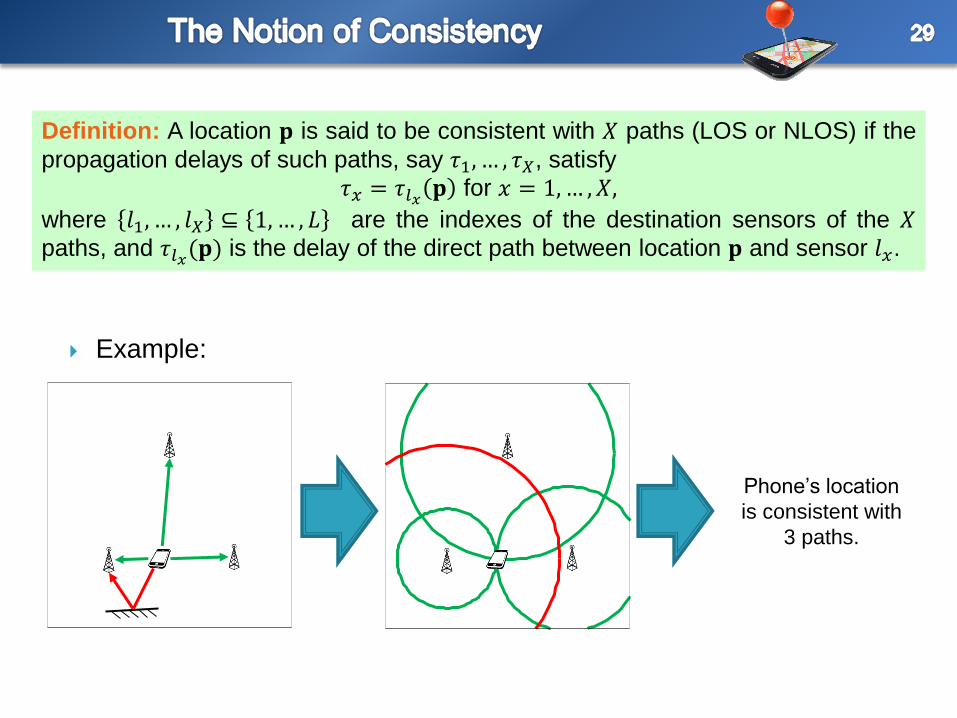
Definition: A location 𝐩 is said to be consistent with 𝑋 paths (LOS or NLOS) if the

propagation delays of such paths, say 𝜏1, … , 𝜏𝑋, satisfy

𝜏𝑥 = 𝜏𝑙𝑥 𝐩 for 𝑥 = 1,… , 𝑋,

where 𝑙1, … , 𝑙𝑋 ⊆ 1,… , 𝐿 are the indexes of the destination sensors of the 𝑋 paths, and 𝜏𝑙𝑥(𝐩) is the delay of the direct path between location 𝐩 and sensor 𝑙𝑥.

Phone’s location

is consistent with

3 paths.

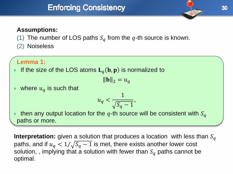
Assumptions:

(1) The number of LOS paths 𝑆𝑞 from the 𝑞-th source is known.

(2) Noiseless

Lemma 1:

If the size of the LOS atoms 𝐋𝑞 𝐛, 𝐩 is normalized to

𝐛 2 = 𝑢𝑞

where 𝑢𝑞 is such that

𝑢𝑞 <1

𝑆𝑞 − 1,

then any output location for the 𝑞-th source will be consistent with 𝑆𝑞 paths or more.

Interpretation: given a solution that produces a location with less than 𝑆𝑞

paths, and if 𝑢𝑞 < 1 𝑆𝑞 − 1 is met, there exists another lower cost

solution, , implying that a solution with fewer than 𝑆𝑞 paths cannot be optimal.

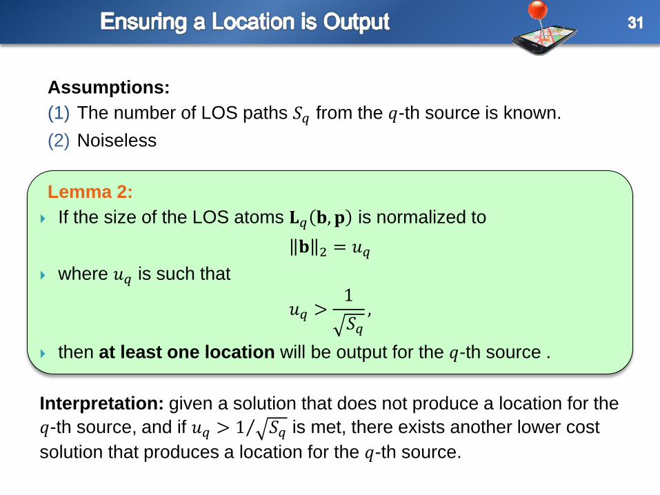
Assumptions:

(1) The number of LOS paths 𝑆𝑞 from the 𝑞-th source is known.

(2) Noiseless

Lemma 2:

If the size of the LOS atoms 𝐋𝑞 𝐛, 𝐩 is normalized to

𝐛 2 = 𝑢𝑞

where 𝑢𝑞 is such that

𝑢𝑞 >1

𝑆𝑞,

then at least one location will be output for the 𝑞-th source .

Interpretation: given a solution that does not produce a location for the

𝑞-th source, and if 𝑢𝑞 > 1 𝑆𝑞 is met, there exists another lower cost

solution that produces a location for the 𝑞-th source.

Assumptions:

(1) The number of LOS paths 𝑆𝑞 from the 𝑞-th source is known.

(2) Noiseless

(3) Only the true location of the 𝑞-th source is consistent with 𝑆𝑞 paths.

Theorem:

If the size of the LOS atoms 𝐋𝑞 𝐛, 𝐩 is normalized to

𝐛 2 = 𝑢𝑞

where 𝑢𝑞 is such that 1

𝑆𝑞 − 1< 𝑢𝑞 <

1

𝑆𝑞 − 1,

then by Lemma 1 and 2, a location will be output for the 𝑞-th source

that is consistent with 𝑆𝑞 paths, and by Assumption (3) it must be the

correct location.

𝑆1 = 4

Define 𝑣 = 1 𝑢1 2

By Theorem: 𝑆1 − 1 < 𝑣 < 𝑆1

Minimize atomic

norm and recover

sources locations

Relaxing assumption 𝑆𝑞 is known.

◦ 𝑆 𝑞 initial guess # LOS paths for source 𝑞.

◦ If 𝑢𝑞 is chosen such that 1

𝑆 𝑞−1< 𝑢𝑞 <

1

𝑆 𝑞−1 where 𝑆 𝑞 > 𝑆𝑞…

…no location will be output for source 𝑞.

If 𝐩 𝑞 = 𝑆 𝑞 𝑆 𝑞 − 1

for any 𝑞

𝑆 𝑞 = 𝐿

for all 𝑞

Stop if 𝐩 𝑞 ≠ for all 𝑞

Optimization problem is ∞-dimensional:

min𝑐𝑘𝑞,𝑐𝑘𝑞𝑙. 𝑐𝑘

𝑞

𝑘

+ 𝑐𝑘𝑞𝑙

𝑘

subject to: 𝐑 − 𝑐𝑘𝑞𝐋𝑞 𝐩𝑘

𝑞

𝑘

𝑄

𝑞=1

+ 𝑐𝑘𝑞𝑙𝐍𝑞𝑙 𝜏𝑘

𝑞𝑙

𝑘

𝐿

𝑙=1

𝑄

𝑞=12

≤ 𝜖

Grid approach (converges to original problem [Rang,Bhaskar,Recht’13])

𝐩𝑘𝑞∈

𝜏𝑘𝑞𝑙∈

Search area

2D

0 Max delay

∞ locations and ∞ delays

∞ atoms

Create

grids

𝐩𝑘𝑞∈

𝜏𝑘𝑞𝑙∈

Search area

2D

0 Max delay

Finite # locations and # delays

finite # atoms

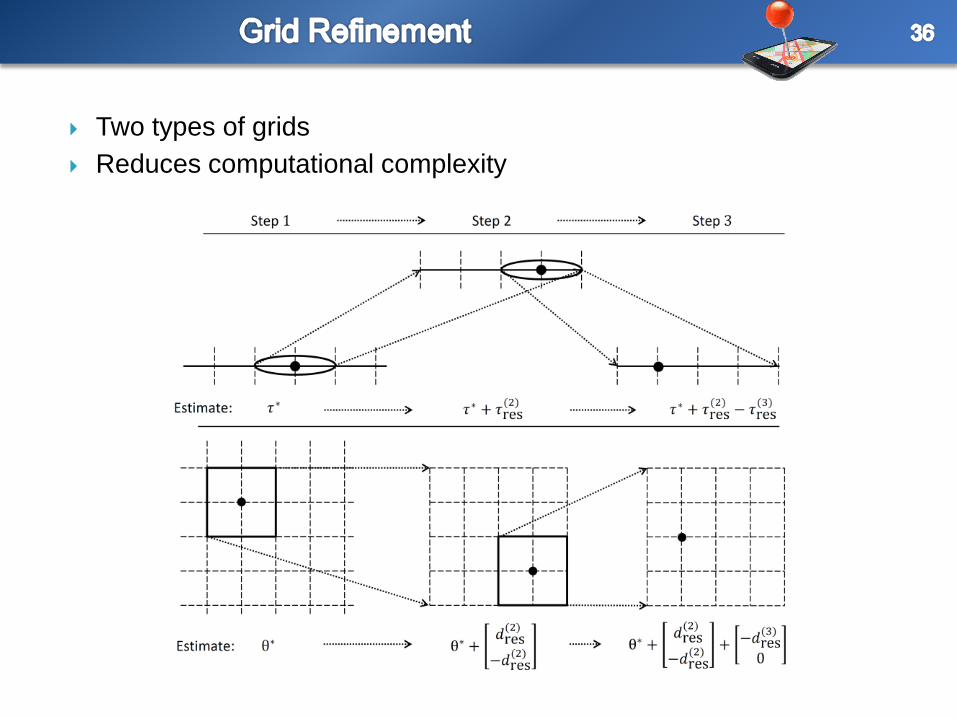
Two types of grids

Reduces computational complexity

10 MHz emitter (30 m ranging resolution)

Multipath channel RMS delay spread is 500 ns (exponential profile,

Poisson arrivals)

Search area: 200 x 200 m

5 base stations and 1 UE

100 samples/sensor

Sensor with blocked LOS

Correct recovery if error is smaller than 10 m

Error normalized to 30 m

SNR = 30 dB per observation window (100 samples and 5

sensors)

SNR = 30 dB per observation window

SNR = 30 dB per observation window

Resources allocation for MIMO radar

Algorithms for power and/or bandwidth allocation in the presence

of multiple targets are provided.

Bandwidth allocation shown to be more valuable than power

allocation.

A novel approach for localization of emitters in multipath featuring

Direct localization outperforms classical TOA indirect localization

An approximation of ML estimator

+ novel framework captures additional information:

Sparse multipath

LOS are first arrivals

Sparse # sources

LOS signals originate from a common emitter location

Multipath is local

Does not require channel state information, such as power

delay profile

Cloud-based

Computationally more expensive than indirect techniques but…

…Grid refinement approach proposed for reduced complexity