2012 Orange County Sanitation District (OCSD) Outfall...
23
2012 Orange County Sanitation District (OCSD) Outfall Diversion – Lessons Learned Report Eric Terrill, Principal Investigator Leslie Rosenfeld, Principal Investigator SCCOOS Technical Director CeNCOOS Program Director Scripps Institution of Oceanography Monterey Bay Aquarium Research Institute University of California, San Diego 7700 Sandholdt Road 9500 Gilman Drive, Mail Code 0214 Moss Landing, CA 95039 La Jolla, CA 92093-0213 (831) 775-2126 (858) 822-3101 [email protected] [email protected] Julie Thomas, Co-Investigator John Largier, Co-Investigator SCCOOS Executive Director Professor / CeNCOOS Principal Investigator Scripps Institution of Oceanography Bodega Marine Laboratory University of California, San Diego University of California, Davis 9500 Gilman Drive, Mail Code 0214 P.O. Box 247 La Jolla, CA 92093-0214 Bodega Bay, CA 94923 (858) 534-3034 (707) 875-1930 [email protected] [email protected] Anne Footer, Financial Representative Peter Rogowski, Lead Author Marine Physical Laboratory (MPL) Postdoctoral Researcher Scripps Institution of Oceanography Scripps Institution of Oceanography University of California, San Diego University of California, San Diego 291 Rosecrans Street 9500 Gilman Drive, Mail Code 0214 San Diego, CA 92106 La Jolla, CA 92093-0214 (858) 534-1802 (858 822-0681 [email protected] [email protected] March 25, 2014
-
Upload
duongkhanh -
Category
Documents
-
view
214 -
download
0
Transcript of 2012 Orange County Sanitation District (OCSD) Outfall...
2012 Orange County Sanitation District (OCSD) Outfall Diversion – Lessons Learned Report
Eric Terrill, Principal Investigator Leslie Rosenfeld, Principal Investigator
SCCOOS Technical Director CeNCOOS Program Director
Scripps Institution of Oceanography Monterey Bay Aquarium Research Institute
University of California, San Diego 7700 Sandholdt Road
9500 Gilman Drive, Mail Code 0214 Moss Landing, CA 95039
La Jolla, CA 92093-0213 (831) 775-2126
(858) 822-3101 [email protected]
Julie Thomas, Co-Investigator John Largier, Co-Investigator
SCCOOS Executive Director Professor / CeNCOOS Principal Investigator
Scripps Institution of Oceanography Bodega Marine Laboratory
University of California, San Diego University of California, Davis
9500 Gilman Drive, Mail Code 0214 P.O. Box 247
La Jolla, CA 92093-0214 Bodega Bay, CA 94923
(858) 534-3034 (707) 875-1930
[email protected] [email protected]
Anne Footer, Financial Representative Peter Rogowski, Lead Author
Marine Physical Laboratory (MPL) Postdoctoral Researcher
Scripps Institution of Oceanography Scripps Institution of Oceanography
University of California, San Diego University of California, San Diego
291 Rosecrans Street 9500 Gilman Drive, Mail Code 0214
San Diego, CA 92106 La Jolla, CA 92093-0214
(858) 534-1802 (858 822-0681
[email protected] [email protected]
March 25, 2014
Table of Contents
2012 Orange County Sanitation District (OCSD) Outfall Diversion – Lessons Learned Report ...........1
I. Introduction ...............................................................................................................................................3
II. Sampling Summary ...................................................................................................................................4
III. Recommendations .....................................................................................................................................6
A. Daily Decision Aids ................................................................................................................................. 6
B. Pre-Diversion ........................................................................................................................................... 7
C. Diversion .................................................................................................................................................. 7
D. Post-Diversion Analysis ........................................................................................................................... 8
E. Additional Recommendations .................................................................................................................. 9
IV. Study Assets ..............................................................................................................................................9
A. Near Real-Time ...................................................................................................................................... 10
High Frequency (HF) Radar Derived Surface Currents – Eric Terrill, SIO ................................................ 10
Moorings...................................................................................................................................................... 10
B. Delayed Mode ........................................................................................................................................ 13
Autonomous Profiling Gliders – Burt Jones, Burt Jones Laboratory, USC ................................................ 13
Drifters – Carter Ohlmann, UCSB .............................................................................................................. 13
REMUS AUV – Eric Terrill, SIO ............................................................................................................... 15
Satellites – Ben Holt, NASA JPL ................................................................................................................ 16
Water Quality Sampling Stations ................................................................................................................ 17
C. Self Contained ........................................................................................................................................ 19
Current Profilers - George Robertson, OCSD ............................................................................................. 19
D. Models .................................................................................................................................................... 21
Southern California Bight (SCB) Models – Yi Chao, RSS ......................................................................... 21
E. Web Portal .............................................................................................................................................. 22
V. References ...............................................................................................................................................23
I. Introduction
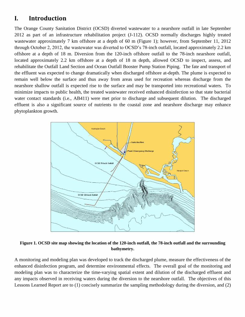
The Orange County Sanitation District (OCSD) diverted wastewater to a nearshore outfall in late September
2012 as part of an infrastructure rehabilitation project (J-112). OCSD normally discharges highly treated
wastewater approximately 7 km offshore at a depth of 60 m (Figure 1); however, from September 11, 2012
through October 2, 2012, the wastewater was diverted to OCSD’s 78-inch outfall, located approximately 2.2 km
offshore at a depth of 18 m. Diversion from the 120-inch offshore outfall to the 78-inch nearshore outfall,
located approximately 2.2 km offshore at a depth of 18 m depth, allowed OCSD to inspect, assess, and
rehabilitate the Outfall Land Section and Ocean Outfall Booster Pump Station Piping. The fate and transport of
the effluent was expected to change dramatically when discharged offshore at-depth. The plume is expected to
remain well below the surface and thus away from areas used for recreation whereas discharge from the
nearshore shallow outfall is expected rise to the surface and may be transported into recreational waters. To
minimize impacts to public health, the treated wastewater received enhanced disinfection so that state bacterial
water contact standards (i.e., AB411) were met prior to discharge and subsequent dilution. The discharged
effluent is also a significant source of nutrients to the coastal zone and nearshore discharge may enhance
phytoplankton growth.
Figure 1. OCSD site map showing the location of the 120-inch outfall, the 78-inch outfall and the surrounding
bathymetry.
A monitoring and modeling plan was developed to track the discharged plume, measure the effectiveness of the
enhanced disinfection program, and determine environmental effects. The overall goal of the monitoring and
modeling plan was to characterize the time-varying spatial extent and dilution of the discharged effluent and
any impacts observed in receiving waters during the diversion to the nearshore outfall. The objectives of this
Lessons Learned Report are to (1) concisely summarize the sampling methodology during the diversion, and (2)
make recommendations for future diversion projects, based on experience from this OCSD diversion. For a
more comprehensive report that covers all aspects of the project (e.g. instrumentation specifics, asset maps,
contact information), the interested reader is refer to the 2012 OSCD Outfall Diversion Summary Report.
This Lessons Learned Report fulfills the request from OCSD that the Southern California Coastal Ocean
Observing System (SCCOOS) and the Central and Northern California Ocean Observing System (CeNCOOS)
provide a summary of results of the diversion’s modeling and monitoring activities and a technical review of the
work performed to determine project recommendations for future diversion studies. The work was conducted by
multiple institutions (Table 1).
Table 1. OCSD 2012 Diversion participant list.
Principle Investigator Affiliation Work Performed Funding
Dave Caron/Caron
Laboratory
University of Southern
California (USC)
Phytoplankton Response J-112 and
NOAA
ECOHAB
Yi Chao Remote Sensing Solutions,
Inc. (RSS)
Regional Ocean Modeling System
(ROMS)
J-112
Ben Holt Jet Propulsion Laboratory
(JPL)
Satellite Support Imagery J-112
Meredith Howard Southern California Coastal
Water Research Project
(SCCWRP)
Project Management and investigator
on the NOAA ECOHAB grant
NOAA
ECOHAB
and SCCWRP
Burt Jones/Jones
Laboratory
University of Southern
California (USC)
Slocum Gliders and near real-time
water quality moorings
J-112 and
NOAA
ECOHAB Grant
Raphael Kudela University of California,
Santa Cruz (UCSC)
Robotic submarine gliders, surface
glider and other moored instruments
NOA ECOHAB
and NSF Grant
Andrew Lucas Scripps Institution of
Oceanography (SIO)
Wire Walkers NOAA
ECOHAB Grant
Carter Ohlman University of California,
Santa Barbara (UCSB)
Drifters J-112
George Robertson Orange County Sanitation
District (OCSD)
Offshore Sampling J-112
John Ryan Monterey Bay Aquarium
Research Institute (MBARI)
Environmental Sample Processor
(ESP)
NOAA
ECOHAB
Eric Terrill Scripps Institution of
Oceanography (SIO)
HF Radar, Telemetered Buoy, and
AUV Mission
J-112
Michael Von
Winklemann
Orange County Sanitation
District (OCSD)
In-Plant Sampling and Nearshore
Sampling
J-112
II. Sampling Summary
The sampling program was comprised of four parts: in-plant, nearshore waters, offshore near-outfall waters, and
offshore regional scale:
In-Plant: The enhanced disinfection program’s effectiveness was monitored by sampling the pre-discharge
effluent (in-plant) up to four times daily. Values for the total and fecal coliform and enterococci bacteria were
predominantly below their respective geometric and single sample means. No trends or changes were seen in
ammonia values.
Nearshore: Daily shoreline sampling for three fecal indicator bacteria (FIB; total coliform, fecal coliform and
enterococci), temperature and salinity occurred at 17 surf-zone stations located along the shore from Sunset
Beach to Crystal Cove.
Surf-zone water temperatures typically fell between 17 and 21 °C and did not appear to be affected by the
discharge plume. Two regional drops in water temperature were seen on September 15 and 29, coinciding with
spring tides. Salinity also did not illustrate impacts from the discharge plume with similar changes occurring
throughout the region during spring tides.
Total coliform counts along the coast were all below the single sample standard of 10,000 MPN/100 mL and,
with few exceptions, single-sample counts were also below the 30-day geometric mean standard of 1,000. No
changes were seen in either temporal or spatial patterns due to the diversion. Greater variability and higher
values were seen primarily from 9N to 3N and were consistent with the occurrence of spring tide events.
Similar patterns were seen in fecal coliform bacteria counts.
Enterococci bacteria showed more variability than either total or fecal coliform bacteria. In addition single
sample standards were exceeded on several occasions and at multiple stations. However, similar to the two
coliform bacteria, the temporal and spatial patterns did not change during the diversion.
Offshore Near-Outfall: An integrated approach was used to characterize the discharge plume and determine its
impacts on the receiving waters.
One telemetered mooring consisting of an integrated Acoustic Doppler Current Profiler (ADCP) and
temperature string was deployed prior to the diversion near the short outfall diffusers to monitor time-
varying ocean currents and temperature. Two telemetered Water Quality Monitoring (WQM) buoys
were also deployed up- and downcoast of the short outfall to measured biologic and optical (bio-optical)
water properties in surface waters. Co-located with the WQM buoys were two current profilers housed
in trawl-resistant bottom mounts (TRBMs). Additionally, three bottom mounted current profilers were
deployed elsewhere in the study area.
To map the spatial extent of the plume, two vessel-based sampling plans and an Autonomous
Underwater Vehicle (AUV) survey were conducted: (i) weekly picket-line sampling of FIB and NH3-N
along the 10 meter (~30 foot) bottom-contour, performed in conjunction with the nearshore (shoreline)
sampling; (ii) CTD profiles and discrete FIB and NH3-N samples at 48 stations located at and
downcurrent of the short outfall – stations were located in two, overlapping 12x4 grids (up- and
downcoast); (iii) a one-day AUV monitoring survey was performed to track the fate and transport of the
wastewater plume under dynamic ambient ocean conditions.
To track surface plume dispersion, water-following drifters were deployed and along-track sampling of
temperature, salinity and colored dissolved organic matter (CDOM) was done to determine surface
plume concentration and to quantify rates of dilution concurrent with advection trajectories.
Offshore Regional Scale: In addition to local-scale characteristics of the plume (within several kilometers of
the outfall pipe), several methods were utilized to track the plume in the far-field.
Three Webb Slocum electric gliders were utilized during the diversion (two actively deployed while one
was serviced) to monitor the spatial and temporal variability of salinity, temperature, and optical
properties (CDOM, backscatter, chlorophyll, phycoerythrin/rhodamine) of the effluent in the far-field.
Numerical modeling used the Regional Ocean Modeling System (ROMS) code and included 3 nested
domains with increasing spatial resolutions of 750-m, 250-m and 75-m over the region of interest.
Boundary conditions were obtained from an ongoing, operational ROMS model that provides real-time,
data-assimilating physical oceanographic output.
Data were used from two satellites: (i) the Advanced Spaceborne Thermal Emission and Reflection
Radiometer (ASTER), an imaging instrument flown on NASA’s Terra satellite, and (ii) the Advanced
Land Imager (ALI) and Hyperion sensors on NASA’s EO-1 satellite.
III. Recommendations
From a combination of observations and analyses that have been completed to-date, the OCSD monitoring and
modeling project yields the following recommendations for monitoring and modeling of future diversions.
A. Daily Decision Aids The following are a list of components used daily during the OCSD diversion and are recommended for future
diversions to guide in-situ sampling.
A web portal provides a centralized, interactive web presence for performers, decision makers, and the
general public to access information and observations that plays an integral role in a diversion
monitoring program. Daily use of an online webpage that displays near real-time observations can help
guide and adapt monitoring activities for making improved measurements in support of the
diversion. The web portal should include visualization or links to background physical parameters such
as wind, waves, currents, and temperature; daily summaries of monitoring efforts; and data products
such as trajectories or models. Having access to these observations allows participants and program
managers to make educated decisions regarding asset placement and go/no go field operations. The
portal could also have a participant only area to upload and disseminate data between performers that
may not be publicly distributable, but would allow for scientific collaborations. Integrated information
management systems are a critical tool to efficiently assess and manage observational programs and
studies.
The near-real-time ADCP data and trajectory estimates were key decision aids that reduced in-situ
sampling of “non-plume” waters – thus focusing available resources on the plume. It is recommended
that a telemetered mooring containing an ADCP and Conductivity and Temperature (CT) string be a
standard element in future outfall diversions. However, surface plumes are typically very thin and the
first velocity bin of the ADCP used for the OCSD diversion was at ~4 m below the ocean surface. For a
surfacing plume, it is recommended to add an instrument (e.g. Acoustic Doppler Velocimeter, ADV) to
measure the near-surface (~1 m) current velocity which will represent plume motion when present and
thus yield a more accurate surface plume trajectory estimate. As flow offshore may be significantly
different, an additional monitoring buoy could be deployed further offshore to guide in-situ sampling
when the plume moves offshore.
The ROMS and ongoing surface current observations from High Frequency (HF) Radar were used daily
to determine general circulation patterns within the observational domain. A similar model approach
with nesting is recommended, however further analysis is required to assess how well the model flow
patterns and dispersion matched observations at the scale of interest. It is likely that further data
assimilation is required (e.g. 2 km resolution HF radar derived surface currents if available) to reproduce
specific flow features on a daily/tidal time scale. Further, a plume model could be coupled to the ROMS
model to provide plume nowcasts.
The objective for glider observations during the diversion was to receive regional data in near real-time
to be used for daily planning of in-situ sampling. However, glider data transmission was too infrequent
(2-3 days) to be incorporated into daily planning due to the amount of data collected that when
downloaded, would lead to significant operational downtime of the vehicle. It is recommended to use
gliders for regional scale data, but daily data transmissions need to be scheduled so that observations can
be used in planning next-day in-situ sampling.
B. Pre-Diversion Deployment of an ADCP/CT mooring prior to the diversion will provide data on the expected surfacing
of the plume and horizontal excursions. It is recommended that such data be used in a plume model to
yield a priori estimates of plume behavior.
Incubation studies in the laboratory using natural plankton assemblages to examine the response of the
phytoplankton community over several days when subjected to different levels of effluent enrichment
showed the potential for significant phytoplankton blooms. This is low-cost and recommended.
A centralized database for all diversion related observational data is recommended – this will allow a
quicker “spin-up” of high-resolution model grids, advance the assimilation of data into high-resolution
numerical models, and provide daily analysis and graphical representation of data as obtained.
C. Diversion Five bottom mounted ADCPs and one ADCP mounted in a telemetered buoy provided current velocities
in the OCSD diversion region. Some sites were redundant due to inadequate spacing of the instruments.
While at least one telemetered ADCP is highly recommended, deployment of additional ADCPs is
suggested. However it is recommended to optimize the spacing of the ADCPs to better capture the
variability of currents within the region of interest.
Capturing the spatial extent and temporal variability of the plume through boat-based profile
observations was not successful. It is recommended to redesign this aspect of the plan. Potential
alternatives include high-speed surface mapping, with real-time map production (given that the surfaced
plume is the focus of attention), combined with either more rapid profiling (e.g., small boat with YSI
Castaway) or tow/yo profiles from a boat guided by the real-time surface mapping. This work requires a
dedicated (small) vessel. Alternatively, AUV surveys have proven effective at mapping the spatial and
temporal extent of wastewater plumes (Wu et al., 1994; Fletcher, 2001; Ramos et al., 2000, 2002, 2007;
Rogowski et al., 2012). The path of the vehicle can be optimized for in-plume sampling through
utilization of near real-time current data from a telemetered buoy. It is recommended to incorporate
glider data download dumps into the AUV path planning so observations can be monitored in a near
real-time manner (~ hourly), with the goal of providing daily decision aids during a future diversions.
Observations of elevated CDOM signature within the plume proved to be a primary natural tracer for the
OCSD diversion and it is recommended that both CDOM and salinity are used as primary tracers in
future diversions. Temperature observations are also useful.
Drifters used during the OCSD diversion reflected considerable near-field flow complexities in the
surface plume. Use of drifters is recommended to provide surface mapping and real-time support for
operational decisions regarding vessel-based sampling locations and to provide post-diversion dilution
assessment. It is recommended that drifters are also deployed late afternoon and evening to monitor the
effect of the onshore sea breeze (common in California) in advecting the surface plume onshore.
In-plant, nearshore and offshore FIB sampling showed the effectiveness of disinfection and is
recommended as a real-time check on public health risks and post-diversion assessment.
Offshore sampling of nutrients and phytoplankton is recommended to identify any algal bloom events
and, if so, to identify dominant taxa to provide safeguards against impacts of potential harmful algal
blooms. Experience in the OCSD monitoring suggests that algal blooms may not always occur.
Remote sensing from satellites and aircraft has the potential for synoptic imaging of a surfacing
discharge plume. However, reliable collection of these data is not always possible (during the OCSD
diversion satellite imagery was not available daily due to weather and mechanical failures).
Nevertheless, remotely sensed data observed during a diversion may be valuable in post-diversion
assessment – specifically it is worth exploring what plume-relevant information that can be obtained
from multispectral data. It is recommended that alternative remote sensing approaches be explored prior
to future use, e.g., autonomous low-altitude aircraft that can be locally deployed and can remain below
cloud cover (yet high enough to yield useful spatial coverage).
D. Post-Diversion Analysis Further analysis of all data collected during the OCSD diversion is recommended to properly assess the
effectiveness of project components and to refine recommendations of high/medium/low priority monitoring
and modeling actions during future diversions. The following is a list of recommended analyses:
A CDOM dilution analysis: compare the effectiveness of dilution calculations using CDOM data with
more traditional dilution methods (i.e. dilution estimates using salinity or drifter data).
An analysis of why no substantial phytoplankton bloom was observed – reasons may be the rapid
dilution of nutrients, the inhibition of phytoplankton growth by high NH4 levels, the occurrence of a
bloom beyond the area sampled (time delay in bloom should lead to spatial offset), or the interplay
between nutrients and the super-chlorination process (does chlorination inhibit algae growth?).
ROMs comparison studies. Drifter data and ADCP data were not assimilated into the model. It is
recommended to perform a comparison of model results with in-situ observations (ADCP, drifters) to
assess the validity and value of ROMS output as an operational tool. Also, analyses could look at
potential improvement to model results if adequate data are assimilated (e.g., fine-scale HF Radar,
ADCP, drifters).
Analysis of costs of diverse approaches in terms of personnel, boats and equipment and of the value of
benefits accrued from such work – identifying value in daily operations or in post-diversion assessment.
E. Additional Recommendations Due to the shallow depth of the diffusers used for the diversion (~18 m), the discharge plume was
expected to surface continuously. However, in-situ observations during the diversion suggested a
portion of the discharge plume remained at depth. Two potential contributing factors to this are
stratification and diffuser design: post-analysis of diversion data is needed to delineate the mechanism. It
is recommended to monitor stratification throughout the water column near the diverted discharge using
a moored string of CT sensors or wirewalker profiler. The hydrodynamics resulting from the diffuser
design and interaction of the high momentum discharge plume with the ambient waters also needs to be
reviewed and modeled (if no prior plume model exists) prior to a diversion.
Budget considerations are needed for the resources and efforts of PIs to provide analyzed data to the
authors’ of summary documents in a timely fashion to allow for a more thorough review of results
before summary documents are drafted. A post-diversion workshop is recommended to review the
findings by the PIs with the authors’.
Better communication before, during, and after the diversion is needed between all groups involved. A
more centralized monitoring and modeling plan is recommended, with each component having clear
objectives and expected outcomes. Further, it is recommended that a lead investigator (or small group)
be identified that can integrate components, activities and analyses. This person/group would
subsequently develop reports and conduct post-project assessment. Additionally, a table with list all
investigators, assets, and either near real-time or delayed observations and products should be required
for everyone to have a clear understanding of deployed assets, data collection, and generated
products. An interactive online web portal with not only near real-time observations for planning, but
also an interactive link for sharing data would be a helpful tool for collaborations prior, during, and
following the diversion. Visualized data formats should be made available in common data formats
such as .kml/.kmz or image file (.jpg, .gif, .png) for online visualization, and in ascii or
netCDF/THREDDS for distributed data when possible.
Evolving observational instrumentation has the potential to benefit future diversions through collection of
higher resolution spatial and temporal datasets. While not used during the OCSD diversion, the following
observational methods may potentially improve characterization of a surfacing plume:
An optimal mode of sampling that would provide highly resolved but spatially sufficient coverage is an
airborne optical imager. The hyperspectral capabilities of such a sensor enable it to map multiple
properties that can help to characterize the plume.
Spatial characterization of a discharge plume by an array of AUVs using “artificial intelligence” that
uses one or more parameters (e.g. CDOM, Salinity) to track the boundaries of plume tracers could
optimize in-situ sampling by providing real-time updates on the spatial and temporal variability of the
plumes location.
IV. Study Assets
A brief description of the assets used during the 2012 OCSD Diversion is given in the following sections. For a
comprehensive summary of how the assets were utilized the reader is referred to the 2012 OCSD Diversion
Summary Report.
A. Near Real-Time
High Frequency (HF) Radar Derived Surface Currents – Eric Terrill, SIO
Existing displays of HF radar derived surface current maps and surface “particle plume tracking” provided by
the CORDC were made available for data assimilation into the ROMS model and as a navigational decision aid
to help guide water quality sampling, respectively.
Moorings
Three telemetered moorings were deployed to measure and transmit ocean currents and water quality
conditions. One mooring was deployed at the 78-inch outfall to measure currents and water temperature. The
other two moorings, deployed up and downcoast of the short outfall, measured biologic and optical (bio-optical)
properties of the surface waters.
a) SIO Outfall Mooring - Eric Terrill, SIO
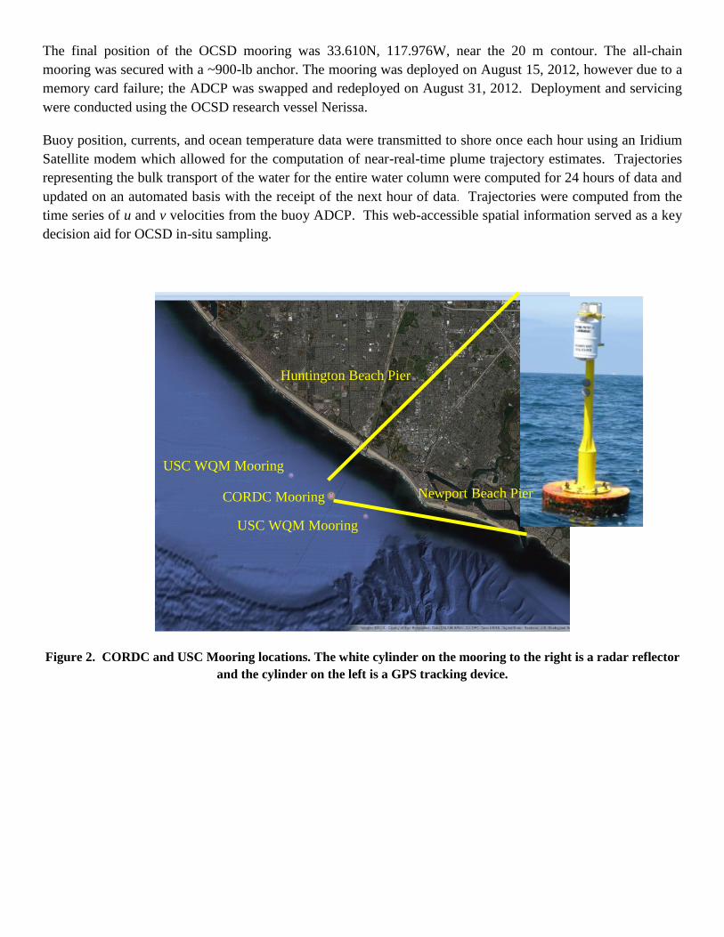
The mooring consisted of a surface buoy that contained an ADCP, (TRDI Instruments, San Diego, CA), a
temperature chain (Precision Measurement Engineering, Encinitas, CA), data logger, satellite telemetry unit,
Global Positioning System (GPS) receiver, and a battery pack. The downward looking ADCP profiled ocean
currents from 4.3 m deep to the seafloor. All mechanical aspects of the buoy, mooring, and anchoring system
were fabricated by Scripps (Figures 2 and 3). The settings for the ADCP are listed in Table 2.
Table 2. Settings for the ADCP used to monitor subsurface currents at OCSD.
System Parameter Setting
Acoustic frequency 600 kHz
Pings per ensemble 50
Ensemble interval 5 minutes
Range cell size 1 meter
Measurement standard deviation 1.4 cm/s
Number of depth cells 25
Measurements of water column stratification were made using temperature sensors located at different depths.
The buoy contained a temperature chain, which consisted of 7 nodes spaced across the water column, each
measuring ocean temperature with accuracy of 0.01°C. Measurements at each depth were synchronized to
provide a water column profile of stratification at one-hour intervals. Use of the interconnected temperature
measurements provided consistent timing across different water depths and eliminated clock drift problems that
often occur when individual, self-recording temperature probes are used. The approximate depths of
measurement were 1.8 m, 5.5 m, 8.2 m, 10.9 m, 12.9 m, 15.2 m, 17.6 m. A series of self-contained temperature
loggers were co-located with the temperature probes and served as a backup to the T-chain.
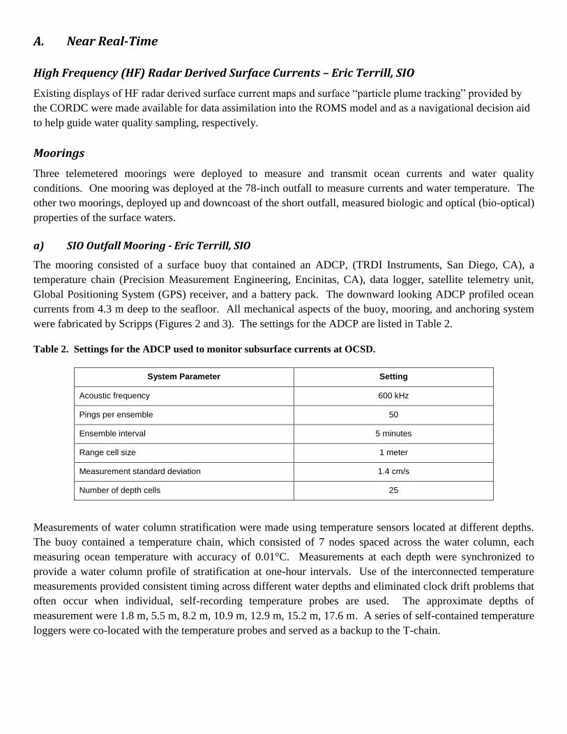
The final position of the OCSD mooring was 33.610N, 117.976W, near the 20 m contour. The all-chain
mooring was secured with a ~900-lb anchor. The mooring was deployed on August 15, 2012, however due to a
memory card failure; the ADCP was swapped and redeployed on August 31, 2012. Deployment and servicing
were conducted using the OCSD research vessel Nerissa.
Buoy position, currents, and ocean temperature data were transmitted to shore once each hour using an Iridium
Satellite modem which allowed for the computation of near-real-time plume trajectory estimates. Trajectories
representing the bulk transport of the water for the entire water column were computed for 24 hours of data and
updated on an automated basis with the receipt of the next hour of data. Trajectories were computed from the
time series of u and v velocities from the buoy ADCP. This web-accessible spatial information served as a key
decision aid for OCSD in-situ sampling.
Figure 2. CORDC and USC Mooring locations. The white cylinder on the mooring to the right is a radar reflector
and the cylinder on the left is a GPS tracking device.
Huntington Beach Pier
Newport Beach Pier
USC WQM Mooring
USC WQM Mooring
CORDC Mooring
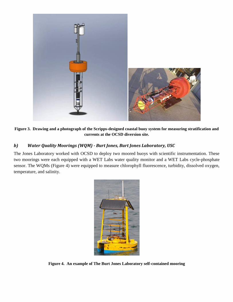
Figure 3. Drawing and a photograph of the Scripps-designed coastal buoy system for measuring stratification and
currents at the OCSD diversion site.
b) Water Quality Moorings (WQM) - Burt Jones, Burt Jones Laboratory, USC
The Jones Laboratory worked with OCSD to deploy two moored buoys with scientific instrumentation. These
two moorings were each equipped with a WET Labs water quality monitor and a WET Labs cycle-phosphate
sensor. The WQMs (Figure 4) were equipped to measure chlorophyll fluorescence, turbidity, dissolved oxygen,
temperature, and salinity.
Figure 4. An example of The Burt Jones Laboratory self-contained mooring
B. Delayed Mode
Autonomous Profiling Gliders – Burt Jones, Burt Jones Laboratory, USC
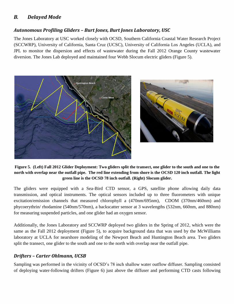
The Jones Laboratory at USC worked closely with OCSD, Southern California Coastal Water Research Project
(SCCWRP), University of California, Santa Cruz (UCSC), University of California Los Angeles (UCLA), and
JPL to monitor the dispersion and effects of wastewater during the Fall 2012 Orange County wastewater
diversion. The Jones Lab deployed and maintained four Webb Slocum electric gliders (Figure 5).
Figure 5. (Left) Fall 2012 Glider Deployment: Two gliders split the transect, one glider to the south and one to the
north with overlap near the outfall pipe. The red line extending from shore is the OCSD 120 inch outfall. The light
green line is the OCSD 78 inch outfall. (Right) Slocum glider.
The gliders were equipped with a Sea-Bird CTD sensor, a GPS, satellite phone allowing daily data
transmission, and optical instruments. The optical sensors included up to three fluorometers with unique
excitation/emission channels that measured chlorophyll a (470nm/695nm), CDOM (370nm/460nm) and
phycoerythrin/ rhodamine (540nm/570nm), a backscatter sensor at 3 wavelengths (532nm, 660nm, and 880nm)
for measuring suspended particles, and one glider had an oxygen sensor.
Additionally, the Jones Laboratory and SCCWRP deployed two gliders in the Spring of 2012, which were the
same as the Fall 2012 deployment (Figure 5), to acquire background data that was used by the McWilliams
laboratory at UCLA for nearshore modeling of the Newport Beach and Huntington Beach area. Two gliders
split the transect, one glider to the south and one to the north with overlap near the outfall pipe.
Drifters – Carter Ohlmann, UCSB
Sampling was performed in the vicinity of OCSD’s 78 inch shallow water outflow diffuser. Sampling consisted
of deploying water-following drifters (Figure 6) just above the diffuser and performing CTD casts following
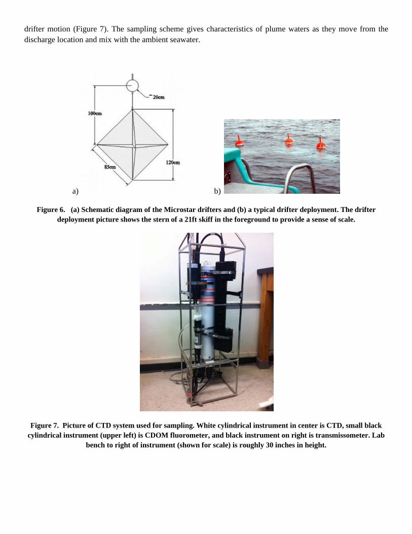
drifter motion (Figure 7). The sampling scheme gives characteristics of plume waters as they move from the
discharge location and mix with the ambient seawater.
a) b)
Figure 6. (a) Schematic diagram of the Microstar drifters and (b) a typical drifter deployment. The drifter
deployment picture shows the stern of a 21ft skiff in the foreground to provide a sense of scale.
Figure 7. Picture of CTD system used for sampling. White cylindrical instrument in center is CTD, small black
cylindrical instrument (upper left) is CDOM fluorometer, and black instrument on right is transmissometer. Lab
bench to right of instrument (shown for scale) is roughly 30 inches in height.
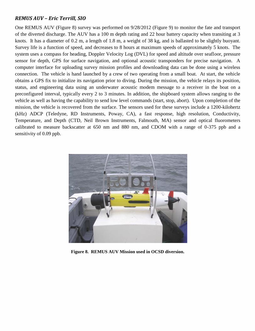
REMUS AUV – Eric Terrill, SIO
One REMUS AUV (Figure 8) survey was performed on 9/28/2012 (Figure 9) to monitor the fate and transport
of the diverted discharge. The AUV has a 100 m depth rating and 22 hour battery capacity when transiting at 3
knots. It has a diameter of 0.2 m, a length of 1.8 m, a weight of 38 kg, and is ballasted to be slightly buoyant.
Survey life is a function of speed, and decreases to 8 hours at maximum speeds of approximately 5 knots. The
system uses a compass for heading, Doppler Velocity Log (DVL) for speed and altitude over seafloor, pressure
sensor for depth, GPS for surface navigation, and optional acoustic transponders for precise navigation. A
computer interface for uploading survey mission profiles and downloading data can be done using a wireless
connection. The vehicle is hand launched by a crew of two operating from a small boat. At start, the vehicle
obtains a GPS fix to initialize its navigation prior to diving. During the mission, the vehicle relays its position,
status, and engineering data using an underwater acoustic modem message to a receiver in the boat on a
preconfigured interval, typically every 2 to 3 minutes. In addition, the shipboard system allows ranging to the
vehicle as well as having the capability to send low level commands (start, stop, abort). Upon completion of the
mission, the vehicle is recovered from the surface. The sensors used for these surveys include a 1200-kilohertz
(kHz) ADCP (Teledyne, RD Instruments, Poway, CA), a fast response, high resolution, Conductivity,
Temperature, and Depth (CTD, Neil Brown Instruments, Falmouth, MA) sensor and optical fluorometers
calibrated to measure backscatter at 650 nm and 880 nm, and CDOM with a range of 0-375 ppb and a
sensitivity of 0.09 ppb.
Figure 8. REMUS AUV Mission used in OCSD diversion.
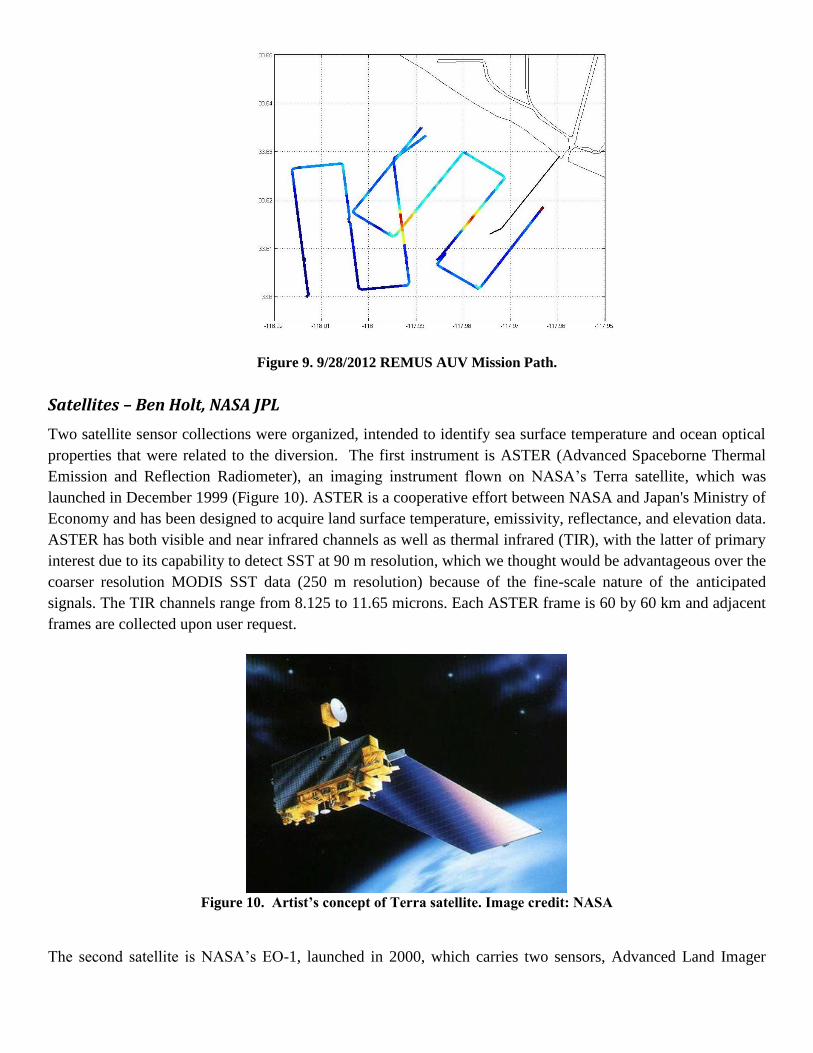
Figure 9. 9/28/2012 REMUS AUV Mission Path.
Satellites – Ben Holt, NASA JPL
Two satellite sensor collections were organized, intended to identify sea surface temperature and ocean optical
properties that were related to the diversion. The first instrument is ASTER (Advanced Spaceborne Thermal
Emission and Reflection Radiometer), an imaging instrument flown on NASA’s Terra satellite, which was
launched in December 1999 (Figure 10). ASTER is a cooperative effort between NASA and Japan's Ministry of
Economy and has been designed to acquire land surface temperature, emissivity, reflectance, and elevation data.
ASTER has both visible and near infrared channels as well as thermal infrared (TIR), with the latter of primary
interest due to its capability to detect SST at 90 m resolution, which we thought would be advantageous over the
coarser resolution MODIS SST data (250 m resolution) because of the fine-scale nature of the anticipated
signals. The TIR channels range from 8.125 to 11.65 microns. Each ASTER frame is 60 by 60 km and adjacent
frames are collected upon user request.
Figure 10. Artist’s concept of Terra satellite. Image credit: NASA
The second satellite is NASA’s EO-1, launched in 2000, which carries two sensors, Advanced Land Imager
(ALI), and Hyperion. ALI is a multispectral sensor with 30 m resolution and a 37 km swath. The Hyperion
sensor is a hyperspectral sensor also with 30 m resolution with a narrow swath of 8 km, which is contained
within the ALI swath. These acquisitions are also obtained upon user request. The requests were done in
conjunction with John Ryan from the Monterey Bay Aquarium Research Institute (MBARI). There was also an
image from HICO, a hyperspectral imager focused on ocean color which is carried onboard the International
Space Station.
Water Quality Sampling Stations
a) Nearshore Water Quality Sampling Stations - George Robertson, OCSD
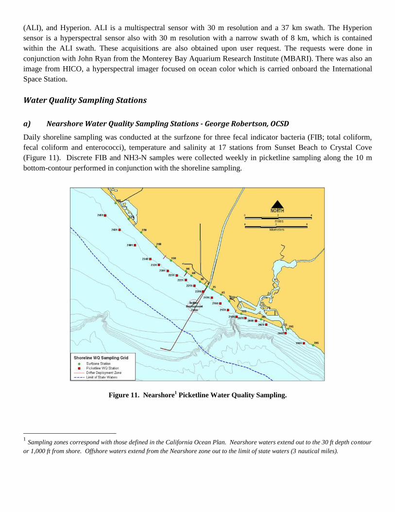
Daily shoreline sampling was conducted at the surfzone for three fecal indicator bacteria (FIB; total coliform,
fecal coliform and enterococci), temperature and salinity at 17 stations from Sunset Beach to Crystal Cove
(Figure 11). Discrete FIB and NH3-N samples were collected weekly in picketline sampling along the 10 m
bottom-contour performed in conjunction with the shoreline sampling.
Figure 11. Nearshore1 Picketline Water Quality Sampling.
1 Sampling zones correspond with those defined in the California Ocean Plan. Nearshore waters extend out to the 30 ft depth contour
or 1,000 ft from shore. Offshore waters extend from the Nearshore zone out to the limit of state waters (3 nautical miles).
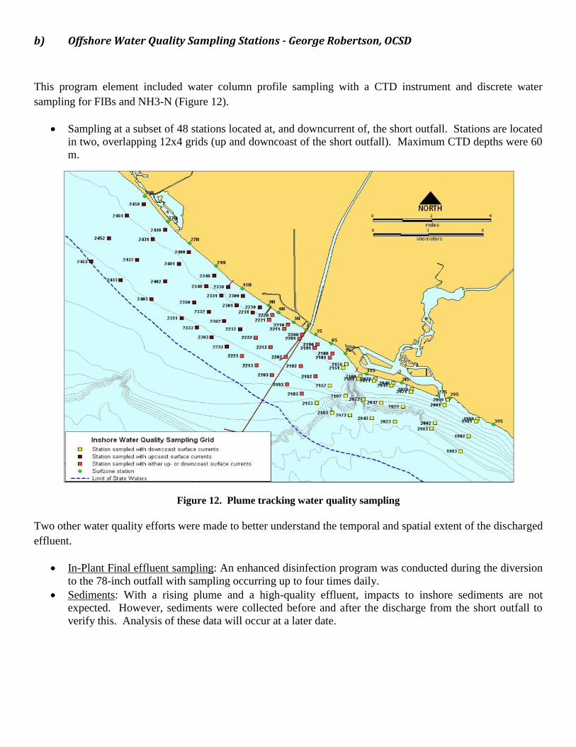
b) Offshore Water Quality Sampling Stations - George Robertson, OCSD
This program element included water column profile sampling with a CTD instrument and discrete water
sampling for FIBs and NH3-N (Figure 12).
Sampling at a subset of 48 stations located at, and downcurrent of, the short outfall. Stations are located
in two, overlapping 12x4 grids (up and downcoast of the short outfall). Maximum CTD depths were 60
m.
Figure 12. Plume tracking water quality sampling
Two other water quality efforts were made to better understand the temporal and spatial extent of the discharged
effluent.
In-Plant Final effluent sampling: An enhanced disinfection program was conducted during the diversion
to the 78-inch outfall with sampling occurring up to four times daily.
Sediments: With a rising plume and a high-quality effluent, impacts to inshore sediments are not
expected. However, sediments were collected before and after the discharge from the short outfall to
verify this. Analysis of these data will occur at a later date.
c) Phytoplankton Response Sampling - Dave Caron, Caron Laboratory, USC
The diversion discharge constituted a significant, localized input of nutrients to the nearshore environment with
potentially major implications for phytoplankton blooms in the nearshore region (See report submitted to OCSD
by Jones and Caron, “Anticipated Biological Response to Extended Discharge from a Nearshore, Shallow
Outfall”).
Two types of studies were conducted to evaluate the response of the local phytoplankton community to this
event:
Experimental studies were conducted twice using natural plankton assemblages contained in bottles to
examine the response of the community over the course of several days when subjected to different
levels of effluent enrichment;
Monitoring (via shipboard and shore sampling and sensing) of the response of the natural phytoplankton
community in the vicinity of the discharge pipe for response to the discharged effluent.
Experimental Field Studies
Two experimental field studies were conducted prior to the diversion event (‘pre-diversion’) and during the
diversion event (‘mid-diversion’) to examine the quantitative and qualitative effects of the OCSD effluent on
natural assemblages of phytoplankton. Seawater for these experiments was collected offshore of the short
outfall (Figure 3.49) at 2 depths for the ‘pre-diversion experiment, the surface (5m) and at the subsurface or
deep chlorophyll maximum (DCM; depth varied) and at 1 depth for the ‘mid-diversion’ experiment, at the
DCM.
Monitoring Studies: Pier Phytoplankton
Water samples were collected weekly from the Newport and Huntington Beach municipal piers situated north
and south of the location of the OCSD effluent pipe sampling to monitor nutrients and phytoplankton
composition.
Monitoring Studies: Vessel Sampling
Offshore samples were collected approximately weekly at a routine grid of stations during OCSD’s offshore
water quality sampling surveys (from OCSD research vessel Nerissa) and at several stations during additional
research cruises aboard the R/V Yellowfin. Samples were collected near-surface and from the subsurface
chlorophyll maximum if one was apparent.
A total of 24 pier samples, 110 samples from the Nerissa, and 72 samples from the Yellowfin were collected as
part of the monitoring studies.
C. Self Contained
Current Profilers - George Robertson, OCSD
Five self-contained current profilers were deployed in TRBMs or tripods (Figure 13). There were two types of
current meters; Acoustic Doppler Current Profilers (ADCP) developed by Teledyne RD Instruments and the
Nortek AWAC current profile, wave height, and direction instrument. The instruments were named after the
moorings that they were deployed next to and the type of instrument installed in the TRBM. Three of the
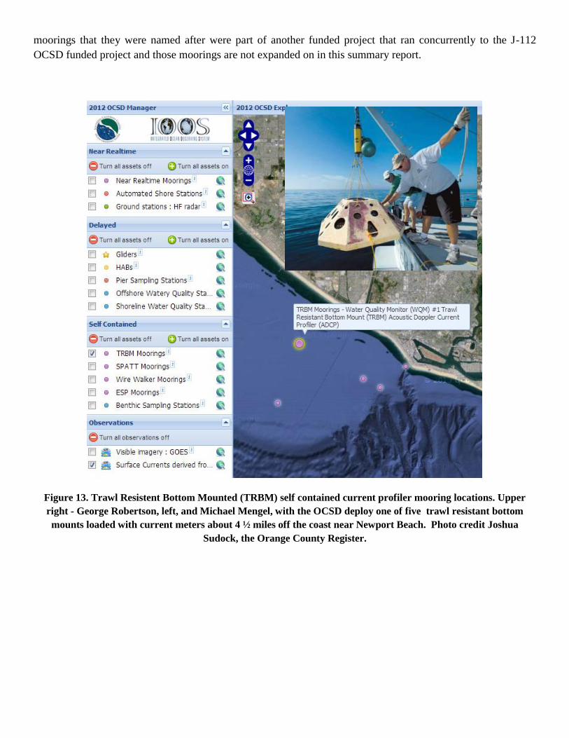
moorings that they were named after were part of another funded project that ran concurrently to the J-112
OCSD funded project and those moorings are not expanded on in this summary report.
Figure 13. Trawl Resistent Bottom Mounted (TRBM) self contained current profiler mooring locations. Upper
right - George Robertson, left, and Michael Mengel, with the OCSD deploy one of five trawl resistant bottom
mounts loaded with current meters about 4 ½ miles off the coast near Newport Beach. Photo credit Joshua
Sudock, the Orange County Register.
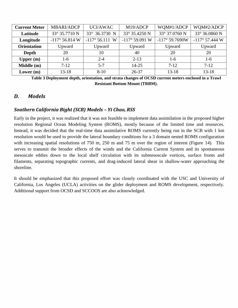
Current Meter MBARI/ADCP UCI/AWAC M19/ADCP WQM#1/ADCP WQM#2/ADCP
Latitude 33° 35.7710 N 33° 36.3730 N 33° 35.4250 N 33° 37.0760 N 33° 36.0860 N
Longitude -117° 56.814 W -117° 56.111 W -117° 59.091 W -117° 59.7690W -117° 57.444 W
Orientation Upward Upward Upward Upward Upward
Depth 20 10 40 20 20
Upper (m) 1-6 2-4 2-13 1-6 1-6
Middle (m) 7-12 5-7 14-25 7-12 7-12
Lower (m) 13-18 8-10 26-37 13-18 13-18
Table 3 Deployment depth, orientation, and strata changes of OCSD current meters enclosed in a Trawl
Resistant Bottom Mount (TRBM).
D. Models
Southern California Bight (SCB) Models – Yi Chao, RSS
Early in the project, it was realized that it was not feasible to implement data assimilation in the proposed higher
resolution Regional Ocean Modeling System (ROMS), mostly because of the limited time and resources.
Instead, it was decided that the real-time data assimilative ROMS currently being run in the SCB with 1 km
resolution would be used to provide the lateral boundary conditions for a 3 domain nested ROMS configuration
with increasing spatial resolutions of 750 m, 250 m and 75 m over the region of interest (Figure 14). This
serves to transmit the broader effects of the winds and the California Current System and its spontaneous
mesoscale eddies down to the local shelf circulation with its submesoscale vortices, surface fronts and
filaments, separating topographic currents, and drag-induced lateral shear in shallow-water approaching the
shoreline.
It should be emphasized that this proposed effort was closely coordinated with the USC and University of
California, Los Angeles (UCLA) activities on the glider deployment and ROMS development, respectively.
Additional support from OCSD and SCCOOS are also acknowledged.
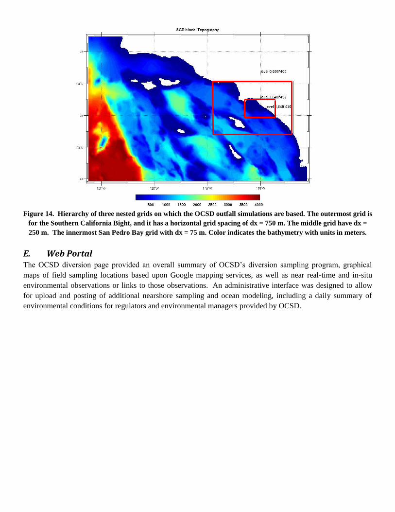
Figure 14. Hierarchy of three nested grids on which the OCSD outfall simulations are based. The outermost grid is
for the Southern California Bight, and it has a horizontal grid spacing of dx = 750 m. The middle grid have dx =
250 m. The innermost San Pedro Bay grid with dx = 75 m. Color indicates the bathymetry with units in meters.
E. Web Portal The OCSD diversion page provided an overall summary of OCSD’s diversion sampling program, graphical
maps of field sampling locations based upon Google mapping services, as well as near real-time and in-situ
environmental observations or links to those observations. An administrative interface was designed to allow
for upload and posting of additional nearshore sampling and ocean modeling, including a daily summary of
environmental conditions for regulators and environmental managers provided by OCSD.
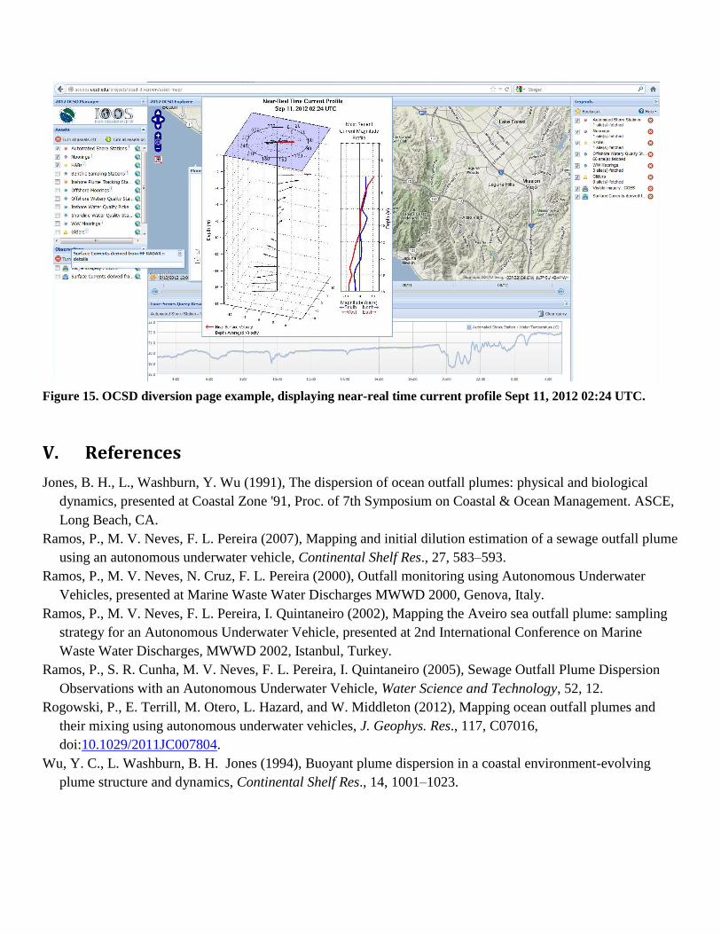
Figure 15. OCSD diversion page example, displaying near-real time current profile Sept 11, 2012 02:24 UTC.
V. References
Jones, B. H., L., Washburn, Y. Wu (1991), The dispersion of ocean outfall plumes: physical and biological
dynamics, presented at Coastal Zone '91, Proc. of 7th Symposium on Coastal & Ocean Management. ASCE,
Long Beach, CA.
Ramos, P., M. V. Neves, F. L. Pereira (2007), Mapping and initial dilution estimation of a sewage outfall plume
using an autonomous underwater vehicle, Continental Shelf Res., 27, 583–593.
Ramos, P., M. V. Neves, N. Cruz, F. L. Pereira (2000), Outfall monitoring using Autonomous Underwater
Vehicles, presented at Marine Waste Water Discharges MWWD 2000, Genova, Italy.
Ramos, P., M. V. Neves, F. L. Pereira, I. Quintaneiro (2002), Mapping the Aveiro sea outfall plume: sampling
strategy for an Autonomous Underwater Vehicle, presented at 2nd International Conference on Marine
Waste Water Discharges, MWWD 2002, Istanbul, Turkey.
Ramos, P., S. R. Cunha, M. V. Neves, F. L. Pereira, I. Quintaneiro (2005), Sewage Outfall Plume Dispersion
Observations with an Autonomous Underwater Vehicle, Water Science and Technology, 52, 12.
Rogowski, P., E. Terrill, M. Otero, L. Hazard, and W. Middleton (2012), Mapping ocean outfall plumes and
their mixing using autonomous underwater vehicles, J. Geophys. Res., 117, C07016,
doi:10.1029/2011JC007804.
Wu, Y. C., L. Washburn, B. H. Jones (1994), Buoyant plume dispersion in a coastal environment-evolving
plume structure and dynamics, Continental Shelf Res., 14, 1001–1023.