23 11

Article 01.1.1Journal of Integer Sequences, Vol. 4 (2001),2

3

6

1

47

The Number-Wall Algorithm: an LFSR Cookbook

W. F. Lunnon

Department of Computer ScienceNational University of IrelandMaynooth, Co. Kildare, Ireland

Email address: fred@cs.may.ie

Abstract

This paper might fairly be said to fall between three stools: the presentation and justification of a numberof related computational methods associated with LFSR sequences, including finding the order, recurrenceand general term; the exploration of tutorial examples and survey of applications; and a rigorous treatmentof one topic, the recursive construction of the number wall, which we believe has not previously appeared.

The Number Wall is the table of Toeplitz determinants associated with a sequence over an arbitraryintegral domain, particularly Z, Fp, R, and their polynomial and series extensions by many variables. Therelation borne by number walls to LFSR (linear recurring shift register) sequences is analogous to that borneby difference tables to polynomial sequences: They can be employed to find the order and recurrence §3,or to compute further terms and express the general term explicitly §10 (although other more elaboratemethods may be more efficient §12, §8).Much of the paper collects and summarizes relevant classical theory in Formal Power Series §1, Linear

Recurrences §2, Pade Blocks (essentially) §3, Vandermonde Interpolation §8, and Difference Tables §9. A‘frame’ relation between the elements of the number wall containing zeros (a non-normal C-table, in Padeterminology) is stated and proved §4, with the resulting recursive generation algorithm and some special cases§5; the consequences of basing the wall on this algorithm instead are explored §6, and a cellular automatonis employed to optimize it in linear time §7.The connections between number walls and classical Pade tables are discussed briefly §11, with other

associated areas (Linear Complexity, QD Algorithm, Toda Flows, Berlekamp-Massey) reviewed even morebriefly §12. Among topics covered incidentally are the explicit number wall for an LFSR, in particular for adiagonal binomial coefficient §8; dealing with high-degree ‘polynomials’ over finite fields, fast computation ofLFSR order over Fp, and the wall of a linear function of a given sequence §9. There are numerous examplesthroughout, culminating in a final gruelingly extensive one §13.Keywords: Number Wall, Zero Window, Persymmetric, Toeplitz Matrix, Hankel Determinant, Linear

Complexity, Finite Field, Cryptographic Security, LFSR, Extrapolation, Toda Flow, Linear Recurring Se-quence, Difference Equation, Zero-Square Table, QD Method, Vandermonde, Formal Laurent Series, PadeTable.

AMS Subject Classification: 94A55, 65D05, 11C20, 65-04, 68Q15, 68Q68, 41A21.

1

0. Introduction and Acknowledgements

The initial aim of this rambling dissertation was to codify what J. H. Conway has christened the NumberWall, an efficient algorithm for computing the array of Toeplitz determinants associated with a sequenceover an arbitrary integral domain: particularly interesting domains in this context are integers Z, integersmodulo a prime Fp, reals R, and their polynomials and power series extensions. §1 (Notation and FormalLaurent Series) sketches elementary the algebraic machinery of these domains and their pitfalls, and §2(LFSR Sequences) summarizes the elementary theory of Linear Feedback Shift Registers.

Our original program is now carried out with an earnest aspiration to rigor that may well appearinappropriate (and may yet be incomplete): however, on numerous occasions, we discovered the hard waythat to rely on intuition and hope for the best is an embarrassingly unrewarding strategy in this deceptivelyelementary corner of mathematical folklore. In §3 (Determinants and Zero-windows) we define the numberwall, give simple algorithms for using it to determine the order and recurrence of an LFSR, establish therecursive construction rule in the absence of zeros (a.k.a. the Sylvester Identity) and the square windowproperty of zeros (a.k.a. the Pade Block Theorem) which, despite of its great age and simplicity of statement,appears to have evaded a substantial number of previous attempts to furnish it with a coherent demonstration.In §4 (The Frame Theorems) we develop the central identities connecting elements around inner and outerframe of a window of zeros in a wall; equally contrary to expectation, these prove to be a notably delicatematter! §5 (The Algorithm, Special Cases) discusses the recursive algorithm implicit in the Frame Theorems,particularly the special cases of an isolated zero and of a binary domain, and digressing along the way toan instructive fallacy which felled a earlier attempted proof. §6 (General Symmetric Walls) explores theconsequences of employing this oddly symmetric algorithm — rather than the original Toeplitz determinant— to build a generalized wall from an arbitrary pair of sequences of variables or numerals. We show thedenominators are always monomial, and that there is arbitrarily large long-range dependence; and give somestriking examples. §7 (Performance and the FSSP) explores how an apparently unrelated idea from CellularAutomaton Theory — Firing Squad Synchronization — plays a major part in tuning a fast computationalalgorithm, which has actually been implemented for the binary domain.

At this point in writing, the focus shifted rather towards a survey of existing methods, as it becameapparent that — while much if not all of this material is known by somebody — there is no collected sourcereference for a whole batch of elementary computational problems associated with LFSRs. §8 (Interpolationand Vandermonde Matrices) summarizes classical material which is used to find explicitly the coefficientsneeded in §10, digressing to give explicitly the wall for binomial coefficient diagonals, and a formula for thegeneral element of the wall in terms of the general element of the sequence in the LFSR case. §9 (DifferenceTables) takes a look at a venerable ancestor, the difference table being to polynomials what the numberwall (in a more general way) is to linear recurrences. Appropriate definition and effective evaluation of apolynomial are nontrivial for finite characteristic; the ensuing investigation leads inter alia to a fast algorithmfor computing the order of an LFSR over Fp, applicable to a recent study of deBruijn sequences. At leastsome of these strands are pulled together in §10 (Explicit Term of an LFSR Sequence) where we discussefficient methods of computing the roots and coefficients of the ‘exponential’ formula for the general elementof an LFSR sequence from a finite set of its elements.

In §11 (Pade Tables) we make the classical connection between number walls and rational approxima-tion, and develop some pleasantly straightforward algorithms for series reciprocal and (‘non-normal’) Padeapproximants. §12 (Applications and Related Algorithms) surveys applications including linear complexityprofiles (LCPs) and numerical roots of polynomials (Rutishauser QD), with a brief description of the well-known Berlekamp-Massey algorithm for computing the recurrence of an LFSR sequence from its elements.Finally §13 (Hideous Numerical Example) features an intimidating computation, intended to illustrate someof the nastier aspects of the Outer Frame Theorem, and succeeding we fear only too well.

As a third strand, we have felt obliged to make this something of a tutorial, and to that end havesketched proofs for the sake of completeness wherever practicable: existing proofs of well-known results inthis area seem often to be difficult of access, incomplete, over-complicated or just plain wrong. We haveincluded frequent illustrative examples, some of which we hope are of interest in their own right; and anumber of conjectures, for this is still an active research area (or would be if more people knew about it).

It would be surprising if much of the material presented here was genuinely new — we have beenscrupulous in acknowledging earlier sources where known to us — but we felt it worth collating under a

2

uniform approach. We originally unearthed the Frame Theorems over 25 years ago, and although the resultmight now quite reasonably be considered to lie in the public domain, to the best of our knowledge nocomplete proof has ever been published. We trust it is at last in a form fit for civilized consumption: ifso, some of the credit should go to the numerous colleagues who have persistently encouraged, struggledwith earlier drafts, and made suggestions gratefully incorporated — in particular Simon Blackburn, DavidCantor, John Conway, Jim Propp, Jeff Shallit, Nelson Stephens.

1. Notation and Formal Laurent Series

For applications we are interested principally in sequences over the integers Z or a finite field Fp, especiallythe binary field. However, to treat these cases simultaneously, as well as to facilitate the proofs, we shall needto formulate our results over an arbitrary ground integral domain, i.e. a commutative ring with unity andwithout divisors of zero. Such a domain may be extended to its field of fractions by Her75 §3.6, permittingelementary linear algebra, matrices and determinants to be defined and linear equations to be solved in theusual way; and further extended to its ring of polynomials and field of (formal) Laurent power series in atranscendental variable, following a fairly routine procedure to be expounded below.There is rarely any need for us to distinguish between variables over these different domains, so they are

all simply denoted by italic capitals. Integer variables (required for subscripts etc, whose values may include±∞ where this makes sense) are denoted by lower-case italic letters. Vectors, sequences and matricesare indicated by brackets — the sequence [Sn] has elements . . . , S0, S1, S2, . . ., and the matrix [Fij ] hasdeterminant |Fij |. A sequence is implicitly infinite in both directions, where not explicitly finite; contextshould suggest if a truncated segment requires extrapolation by zero elements, periodic repetition, or theapplication of some LFSR.In §4 the elements are actually polynomials over the ground domain; and all the quantities we deal with

could be expressed as rational functions (quotients of polynomials) over it. While it is both feasible andconceptually simpler to couch our argument in terms of these, the mechanics of the order notation O(Xk)introduced below become unnecessarily awkward; therefore we prefer to utilize the slightly less familiarconcept of Formal Laurent Series (FLS).We define the field of FLS to be the set of two-sided sequences [. . . , Sk, . . .] whose components lie in

the given ground field, and which are left-finite, that is only finitely many components are nonzero fork < 0. Arithmetic is defined in the usual Taylor-Laurent power-series fashion: that is, addition and negationare term-by-term, multiplication by Cauchy (polynomial) product, reciprocal of nonzeros by the binomialexpansion. The ground field is injected into the extension by S0 → [. . . , 0, S0, 0, . . .].As usual we write an FLS as an infinite sum of integer powers of the transcendental X with finitely

many negative exponents: its generating function. The notation is suggestive, but has to be interpreted withsome care. For instance, we cannot in general map from FLSs to values in the ground field by substitutingsome value for X , since this would require the notion of convergence to be incorporated in the formalism.Fortunately we have no need to do so here, since we only ever specialize X → 0, defined simply as extractingthe component S0 with zero subscript.The following property is deceptively important in subsequent applications.

Theorem: Specialization commutes with FLS arithmetic: that is, if W (V (X), . . .) denotessome (arithmetic) function of FLS elements V (X), . . ., and V (0) denotes V (X) with X → 0etc, then W (V (0), . . .) = W (V (X), . . .)(0).

(1.0)

Proof: This is the case k = 0 of the nontrivial fact that two FLSs U = [. . . , Sk, . . .] and V = [. . . , Tk, . . .] areequal under the operations of field arithmetic (if and) only if they are equal component-wise, that is onlyif Sk = Tk for all k. For suppose there existed distinct sequences [Sk], [Tk] for which U = V arithmetically.Then U − V = 0, where the sequence corresponding to U − V has some nonzero component. Using thebinomial expansion, we calculate its reciprocal; now 1 = (U − V )−1 · (U − V ) = (U − V )−1 · 0 = 0. So thefield would be trivial, which it plainly is not, since it subsumes the ring of polynomials in X.In this connection it is instructive to emphasize the significance of left-finiteness. If this restriction were

abandoned, we could consider say (expanding by the binomial theorem)

U = 1/(1−X) = 1 +X1 +X2 +X3 + . . . ,−V = X−1/(1−X−1) = . . .+X−3 +X−2 +X−1;

3

now by elementary algebra U = V despite the two distinct expansions, and (1.0) would no longer hold.Related to this difficulty is the fact that we no longer have a field: U − V for instance, the constant unitysequence, has no square.

One unwelcome consequence is that the generating function approach frequently employed as in Nie89to discuss Linear Complexity is applicable only to right- (or mut. mut. left-) infinite sequences, and is unableto penetrate the ‘central diamond’ region of a number-wall (§3) or shifted LCP (§12), being restricted to aregion bounded to the South by some diagonal line. [It is noteworthy that, elementary as they might be,these matters have on occasion been completely overlooked elsewhere in the literature.]

Definition: For FLS U , the statement

U = O(Xk)

shall mean that Ul = 0 for l < k.

(1.1)

It is immediate from the definition that

0 = O(X∞);U +O(Xk) = U +O(X l)

for l ≤ k (asymmetry of equality);(U +O(Xk))± (V +O(X l)) = (U ± V ) +O(Xmin(k,l));(U +O(Xk)) · (V +O(X l)) = (U · V ) +O(Xmin(k+n,l+m))

if U = O(Xm) and V = O(Xn);(U +O(Xk))/(V +O(X l)) = (U/V ) +O(Xmin(k−n,l+m))

if in addition Vn 6= 0, so n is maximal.

Notice that we can only let X → 0 in U+O(Xk) if k > 0, otherwise the component at the origin is undefined;and in practice, we only ever do so when also U = O(1). In §4 – §5 we shall implicitly make extensive useof these rules.

For completeness, we should perhaps mention the more usual classical strategy for ensuring that a setof FLSs forms a field: to define convergence and enforce it, say over some annular region of the domain ofcomplex numbers. The connection with our counterexample above is of course that any S, T correspondingto the same meromorphic function in distinct regions will give U − V = 0. The elementary definitions andalgorithms of FLS arithmetic are fully discussed in standard texts such as Hen74 §1.2, or Knu81 §1.2.9and §4.7. With the exception of the thorough tutorial Niv69, these authors consider only the ring of formalTaylor series with exponents k ≥ 0; however, it is a fairly routine matter to extend the ring to a field, andthere seems little reason to constrain oneself in this manner.

4

2. LFSR Sequences

A sequence Sn is a linear recurring or linear feedback shift register (LFSR) sequence when there exists anonzero vector [Ji] (the relation) of length r + 1 such that

r∑

i=0

JiSn+i = 0 for all integers n.

The integer r is the order of the relation. If the relation has been established only for a ≤ n ≤ b− r we saythat the relation spans (at least) Sa, . . . , Sb, with a = −∞ and b = +∞ permitted. LFSR sequences overfinite fields are discussed comprehensively in Lid86 §6.1–6.4.It is usual to write a relation as an auxiliary polynomial J(E) of degree r in the shift operator E : Sn →

Sn+1:

Definition: The LFSR sequence [Sn] satisfies the relation J(E) just when for all n

J(E)[Sn] ≡∑

i

JiEi[Sn] ≡

∑

i

Ji[Sn+i] = [On],

the zero sequence (with order 0 and relation J(E) = 1).

(2.1)

Notice that the number of nonzero components or dimension of a relation as a vector is in general r+1, tworelations being regarded as equal (as for projective homogeneous coordinates) if they differ only by somenonzero constant multiple; also in the case of sequences whose values are given by a polynomial in n §9, thedegree of the polynomial is in general r − 1.The order of a sequence (infinite in both directions) is normally understood to mean the minimum

order of any relation it satisfies; this minimal relation is simply the polynomial highest common factor ofall relations satisfied by the sequence, and is therefore unique. [The existence of such an HCF is guaranteedby the Euclidean property of the ring of polynomials in a single variable E over the ground domain, seeHer75 §3.9.] The leading and trailing coefficients Jr, J0 of the minimal relation J of a (two-way-infinite)sequence are nonzero: such relations we shall call proper. These definitions must be interpreted with carewhen applied to segments with finite end-points, principally because even minimal relations may fail to beproper: both leading and trailing zero coefficients will then need to be retained during polynomial arithmeticon relations. Furthermore, if the minimum order is r and the span has length < 2r, a minimal relation is nolonger unique, since there are too few equations to specify its coefficients.By the elementary theory (Lid86 §6.2) we have an explicit formula for an LFSR sequence:

Theorem: [Sn] satisfies J(E)[Sn] = [On] just when

Sn =∑

i

KiXin for all n,

where the Xi are the roots of J(X) and the Ki are coefficients, both lying in the algebraicclosure of the ground domain when J(X) has distinct roots; when the root Xi occurs withmultiplicity ei, Ki is a polynomial in n of degree ei − 1.

(2.2)

Proof: Since we make frequent reference to this well-known result, we sketch a demonstration for thesake of completeness. [Over ground domains of finite characteristic, it is important that the ‘polynomials’Ki(n) are defined in terms of binomial coefficients; we return to this point in §9.]From the Pascal triangle recursion, by induction on e

(E− 1)(

n

e− 1

)

=

(

n

e− 2

)

,

(E− 1)e(

n

e− 1

)

= 0;

(2.3)

5

and so by expressing the arbitrary polynomial K(n) of degree e− 1 in n as a linear combination of binomialcoefficients, we see that its e-th difference (E − 1)eK(n) is zero. Similary (E − X)Xn = 0 and (E −X)eK(n)Xn = 0 for arbitrary X . Suppose Sn has the explicit form above (2.2), where J(X) has just mdistinct roots; let X ≡ Xm etc., and let primes denote the analogous expressions involving only the otherm− 1 roots; then

J(E)Sn =∏

i

(E−Xi)eiSn

= J ′(E)(

(E−X)eK(n)Xn)

+ (E−X)e(

J ′(E)S′n)

= J ′(E)(0) + (E−X)e(0) = 0

for all n, using induction on m.

The converse can be approached constructively as in Lid86 (who prove the distinct case only) by settingup linear equations for the Ki and showing that they possess a unique solution, as we shall do in (8.6) (fordistinct Xi) and (9.2) (for coincident Xi effectively). In the general case of multiple roots, it is simplerto observe that the set of sequences satisfying a given relation J (assumed to possess nonzero leading andtrailing coefficients) comprise a vector space Her75 §4 whose dimension must be r, since each is completelydetermined by its initial r terms. The set constructed earlier is also a subspace of dimension r, so the twosets are identical by Her75 Lemma 4.1.2.

If J is minimal then all the Ki are nonzero: for the Galois group of an irreducible factor of J is transitiveon those Xi and their corresponding Ki while leaving Sn invariant, so those Ki must all be nonzero or allzero. In the latter case, J may be divided by the factor and so is not minimal. When all the roots coincideat unity, Sn equals an arbitrary polynomial of degree r − 1 in n; so the latter are seen to be a special caseof LFSR sequences.

3. Determinants and Zero-windows

Given some sequence [Sn], we define its Number Wall (also Zero Square Table or — misleadingly — QDTable) [Sm,n] to be the two dimensional array of determinants given by

Definition:

Sm,n =

∣

∣

∣

∣

∣

∣

∣

∣

Sn Sn+1 . . . Sn+mSn−1 Sn . . . Sn+m−1...

.... . .

...Sn−m Sn−m+1 . . . Sn

∣

∣

∣

∣

∣

∣

∣

∣

. (3.1)

The value of Sm,n is defined to be unity for m = −1, and zero for m < −1. [These are known as Toeplitzdeterminants; or, with a reflection making them symmetric, and a corresponding sign change of (−1)(

m+12 ),

as persymmetric or Hankel determinants.] The rows and columns are indexed by m, n resp. in the usualorientation, with the m axis increasing to the South (bottom of page) and n to the East (right). [Forexamples see the end of §5 and elsewhere.]

Lemma: For any sequence [Sn] and integers n and m ≥ 0, we have Sm−1,n 6= 0 andSm,n = 0 just when there is a proper linear relation of minimum order m spanning at leastSn−m, . . . , Sn+m. Its coefficients Ji are unique up to a common factor. Further, when

Sm,n = Sm,n+1 = . . . = Sm,n+g−1 = 0 and Sm,n−1 6= 0, Sm,n+g 6= 0

the relation maximally spans Sn−m, . . . , Sn+m+g−1. [Notice that we may have n = −∞ org = +∞.]

(3.2)

6

Proof: by elementary linear algebra. For g = 1, set up m+ 1 homogeneous linear equations for the Ji,with a unique solution when they have rank m:

Sn−mJ0 + Sn−m+1J1 + . . . + SnJm = 0,

...

SnJ0 + Sn+1J1 + . . . + Sn+mJm = 0,

...

Sn+g−1J0 + Sn+gJ1 + . . . + Sn+m+g−1Jm = 0.

Using Sn−m+1, . . . , Sn+m+1 on the right-hand side instead of Sn−m, . . . , Sn+m leaves m of these equationsunaltered, so by induction on g the solution is constant over the whole segment of [Sn] of length 2m + g,and no further. This solution is proper: for if Jm = 0 there would be a nontrivial solution to the equationswith m replaced by m − 1, and so we should have Sm−1,n = 0 contrary to hypothesis; similarly if J0 = 0.Similarly, it is minimal. Conversely, if a there is a relation, then Sm,n = 0; if it is minimal, then it is unique,and if it is also proper then m cannot be reduced, so Sm−1,n 6= 0.

Corollary: [Sn] is an LFSR sequence of order r if and only if row r (and all subsequentrows) of its number-wall degenerate to the zero sequence, but row r − 1 does not. (3.3)

Given as many terms as we require of an LFSR sequence [Sn], we can use (3.3) to compute its order rfrom its number-wall. Now suppose in addition we require to find the linear relation J(E) which generatesit. We introduce a new sequence of polynomials in a transcendental X over the domain, defined by

Un(X) = (E−X)Sn = Sn+1 −X.Sn,

and form its number wall Um,n(X). If we set X → E, both sequence and wall (for m 6= −1) perforcedegenerate to all zeros; therefore each Um,n(E) is a relation spanning those 2m + 2 elements of [Sn] fromwhich it was computed. Now for degree r there is only one such polynomial (modulo a constant factor),and that is the required minimal relation J(E): for all n therefore, Ur−1,n equals J(X) multiplied by somedomain element (nonzero since setting X → 0 gives the wall for [Sn] itself); and similarly Ur−1,n = 0 on allsubsequent rows m ≥ r.

Corollary: [Sn] is an LFSR sequence of order r if and only if row r (and all subsequentrows) of the number-wall of Sn+1 −X.Sn degenerate to the zero sequence, but row r doesnot; then row r − 1 equals the minimal relation J(X) of [Sn] times a geometric sequenceover the ground domain.

(3.4)

This algorithm is slower than the more sophisticated Berlekamp-Massey method (12.1), taking time of orderr4 arithmetic operations over the ground domain (using straightforward polynomial multiplication) ratherthan r2; but it is noticeably easier to justify, and it also gives the relations of intermediate (odd) spans.A simple recursive rule for constructing the number-wall of a given sequence in the absence of zeros

is classical, and follows immediately from the pivotal condensation rule styled by Ioh82 §1.2 the SylvesterIdentity [described byAit62 §45 as an extensional identity due to Jacobi, and elsewhere credited to Desnanot,Dodgson or Frobenius]:

Lemma: Given an m × m matrix [Fij ] and an arbitrary (m − k) × (m − k) minor [Gij ]where 0 ≤ k ≤ m, define Hij to be the cofactor in |F | selecting all the rows and columns of|G|, together with the i-th row and j-th column not in |G|. Then

|Fij | × |Gij |k−1 = |Hij |.(3.5)

7

Proof: We may suppose the elements of [Fij ] to be distinct variables transcendental over the grounddomain, thus avoiding any problem with singular matrices. We may also suppose the rows and columns of[Fij ] permuted so that [Gij ] occupies the SE corner, i, j > k: this leaves the determinant unaltered exceptfor a possible change of sign. Consider the matrix [Eij ] with Eij being Fij when i > k, or |G| borderedby row i and column j of F when i ≤ k. Expanding this determinant by its first row, we see (with somedifficulty — the reader is advised to work through a small example) that

Eij = |G|Fij +∑

q

AiqFiq ,

where the Aiq are cofactors from the last m− k rows which do not depend on j. So [Eij ] is effectively [Fij ]with each of its first k rows multiplied by |G|, then subjected to a sequence of elementary column operationswhich leave the determinant unaltered. On the one hand then, |E| = |F | × |G|k .Again,

Eij =

Hij for 1 ≤ i ≤ k and 1 ≤ j ≤ k by definition,Gij for k < i ≤ m and k < j ≤ m by definition,0 for 1 ≤ i ≤ k and k < j ≤ m (determinant with equal columns).

So on the other hand |E| = |H | × |G|. Canceling the nonzero |G| from |E| gives the result.

Theorem: A symmetrical relation between the elements of the number-wall is

S2m,n = Sm+1,nSm−1,n + Sm,n+1Sm,n−1.(3.6)

Proof: In (3.5) choose k = 2, |Fij | = Sm+1,n, and |Gij | = Sm−1,n where this last is the cofactoroccupying the interior of [Fij ]. Then the Hij also turn out to be entries in the wall, and we find

Sm+1,n × Sm−1,n =∣

∣

∣

∣

Sm,n Sm,n+1Sm,n−1 Sm,n

∣

∣

∣

∣

.

Corollary: A partial recursive construction for the number-wall is

S−2,n = 0, S−1,n = 1, S0,n = Sn,

Sm,n =(

Sm−1,n2 − Sm−1,n+1Sm−1,n−1)

)

/Sm−2,n for m > 0,

provided Sm−2,n 6= 0.

(3.7)

[The initial row of zeros is not a great deal of use at this point, but comes in useful later as an outer framefor zeros occurring in the sequence.]The possibility of zero elements in the wall is a stumbling block to the use of (3.7) for its computation,

particularly if the ground domain happens to be a small finite field, when they are almost certain to occur.The next result sharpens a classical one in the study of Pade Tables §11, the first half of the ‘Pade BlockTheorem’. All proofs of it (including this author’s) should be regarded with suspicion, having a disconcertingtendency to resort to hand-waving at some crucial point in the proceedings: for this reason we feel regretfullyunable to recommend a prior version.A region of a number wall is defined to be a simply-connected subset of elements, where two elements

are connected when they have one subscript (m or n) equal, the other (n or m) differing by unity. Theregions which we consider are g× g′ rectangles, having at most four boundary segments along each of whichsome subscript is constant; their lengths g, g′ (measured in numbers of elements along each segment) mayrange from zero to infinity. The inner frame of a rectangle is the smallest connected set which disconnects the

8

region from its complement: it normally comprises four edges and four corners. The outer frame similarlydisconnects the union of the rectangle with its inner frame from the complement. [In the example at the endof §5 will be found a 4× 4 (square) rectangle of zeros, with an inner frame of ones.]

Theorem: Square Window Theorem: Zero elements Sm,n = 0 of a number-wall occur onlywithin zero-windows, that is square g× g regions with nonzero inner frames. The nullity of(the matrix corresponding to) a zero element equals its distance h from the inner frame.

(3.8)

Proof: To start with, by (3.6) if Sm−1,n = Sm,n−1 = 0 then Sm,n = 0, and by (3.6) shifting m ←m− 1, n← n− 1, similarly Sm−1,n−1 = 0; the mirror-image argument yields the converse. Now by an easyinduction, any connected region of zeros must be a (possibly infinite) rectangle.Now let there be such a rectangle with g rows, g′ columns, and NW corner (n increasing to the East

and m to the South) located at Sm,n: in detail,

Sm,n = 0, . . . , Sm,n+g′−1 = 0;

Sm,n = 0, . . . , Sm+g−1,n = 0,

Sm,n+g′−1 = 0, . . . , Sm+g−1,n+g′−1 = 0,

Sm+g−1,n = 0, . . . , Sm+g−1,n+g′−1 = 0,

Sm−1,n 6= 0, . . . , Sm−1,n+g′ 6= 0;Sm,n 6= 0, . . . , Sm+g,n 6= 0;

Sm,n+g′ 6= 0, . . . , Sm+g,n+g′ 6= 0;Sm+g,n 6= 0, . . . , Sm+g,n+g′ 6= 0.

Then by (3.2) a unique minimal relation J(E) of order m spans Sn−m, . . . , Sn+m+g−1. Suppose g′ > g: then

the relation EgJ of order m+ g spans Sn−m−g, . . . , Sn+m+g, so by (3.2) Sm+g,n = 0, contrary to hypothesis.Suppose g′ < g: then since Sm+g′,n = 0, there is a relation spanning Sn−m−g′ , . . . , Sn+m+g′ ; also sinceSm+g′−1,n−1 6= 0 is a nonzero minor of Sm+g′,n, the latter has nullity 1 and the relation must thereforebe unique. One such relation is simply Eg

′

J : so J spans Sn−m+g′ , . . . , Sn+m+g′ and by (3.2) Sm,n+g′ = 0,contrary to hypothesis. The only possibility remaining is that g′ = g, and the rectangle must be a square.Consider this square divided by its diagonals i − j = m − n and i + j = m + n + g − 1 into North,

East, South, West quarters; let h denote the distance of the element Si,j from the frame in the samequarter. All the elements in the North quarter have rank m, since the only relations spanning subintervalsof Sn−m, . . . , Sn+m+g−1 are (polynomial) multiples of J itself: in particular, if g is odd, the central elementhas rank m and nullity h = [(g + 1)/2]. If g is even, there are four elements at the centre, the North pairhaving rank m and nullity h as before; the South pair have rank m + 1, since (for example) any relationcorresponding to Sm+g/2,n+g/2−1 spans Sm−n−1, . . . , Sn+m+g/2, but Sm−n−1 lies outside the span of J (therelations are multiples of EJ). So for any g the central elements have nullity equal to their distance hfrom the frame. Now observe that the nullity of any element Si,j can only differ from that of its neighborsSi−1,j , Si,j−1, Si,j+1, Si+1,j by at most unity, since the matrices differ essentially by a single row or column.Therefore it must decrease with h in all directions, in order to reach zero with h at the inner frame whereall elements are nonzero.A simple consequence of (3.8) is the occurrence of ‘prime windows’ in a wall over some larger ground

domain:

Corollary: Elements divisible by some prime ideal P clump together in square regions,elements at distance h from the frame being divisible by (at least) P h.

(3.9)

In particular, these windows are noticeable for ordinary primes p in integer walls.A less obvious but more useful and rather elegant consequence, credited to Massey in Cha82, quantifies

the notion that, if two different sequences have a large common portion, then at least one of them has highlinear order. It could be proved directly by linear dependence arguments.

Corollary: Massey’s Lemma: The sum of the orders of proper relations spanning twointervals of a sequence exceeds the length of the intersection, unless each relation spanstheir union.

(3.10)

9

Proof: Let the intervals (ai, bi) of the sequence be spanned maximally by minimal proper relations of ordersri, for i = 1, 2. By (3.2), (3.8) there are corresponding windows in the number-wall at (mi, ni) of size giwhere ai = ni −mi, bi = ni +mi + gi − 1, so

mi = ri, ni = ai + ri, gi = bi − ai − 2ri + 1.

Suppose the windows to be distinct (failing which their parameters coincide in pairs); since they are squareand cannot overlap, one of the following is true:

m1 + g1 < m2, n1 + g1 < n2, m2 + g2 < m1, n2 + g2 < n1.

Substituting, either

b1 − a1 − r1 + 1 < r2 orb1 − r1 + 1 < a2 + r2 orb2 − a2 − r2 + 1 < r1 orb2 − r2 + 1 < a1 + r1

whencer1 + r2 > 1 +min(b1 − a1, b1 − a2, b2 − a2, b2 − a1).

as claimed.Relaxing the maximality constraint on the intervals and the minimality on the order does not affect the

result.As an illustration, suppose we are to find the order and relation spanning

S = [0, 0, 0, 1, 16, 170, 1520, 12411, 96096, 719860, . . .].

The following pair of number-walls can be computed via (3.6): The final row of zeros of the first suggests(3.3) that the order might be r = 4. The final row of the second gives (3.4) the auxiliary polynomialJ = E4 − 16E3 + 86E2 − 176E+ 105 = 0, that is S satisfies the relation

Sn+4 − 16Sn+3 + 86Sn+2 − 176Sn+1 + 105Sn = 0.

m\n 0 1 2 3 4 5 6 7 8 9

−2 0 0 0 0 0 0 0 0 0 0−1 1 1 1 1 1 1 1 1 1 10 0 0 0 1 16 170 1520 12411 96096 7198601 0 0 0 1 86 4580 200530 7967001 3002587562 0 0 0 1 176 21946 2449616 2628488113 1 105 11025 1157624 0 0

0 0 0 0 0 0 0

1 1 1 1 1 1 1

0 0 1 16−X 170−16X 1520−170X 12411−1520X

0 0 1 86−16X+X2 4580−1200X+86X2 200530−59824X+4580X2

1 176−86X+16X2−X3 21946−13456X+2711X2−176X3

105−176X+86X2−16X3+X4

10

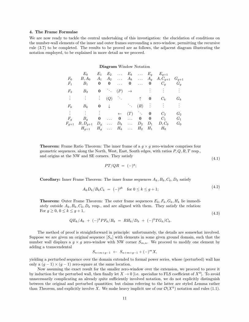
4. The Frame Formulae

We are now ready to tackle the central undertaking of this investigation: the elucidation of conditions onthe number-wall elements of the inner and outer frames surrounding a zero-window, permitting the recursiverule (3.7) to be completed. The results to be proved are as follows, the adjacent diagram illustrating thenotation employed, to be explained in more detail as we proceed.

Diagram Window Notation

E0 E1 E2 . . . Ek . . . Eg Eg+1F0 B,A0 A1 A2 . . . Ak . . . Ag A,Cg+1 Gg+1F1 B1 0 0 . . . 0 . . . 0 Cg Gg

F2 B2 0. . . (P ) →

......

......

...... (Q)

. . . ↑ 0 Ck Gk

Fk Bk 0 ↓ . . . (R)...

......

......

... ← (T ). . . 0 C2 G2

Fg Bg 0 . . . 0 . . . 0 0 C1 G1Fg+1 B,Dg+1 Dg . . . Dk . . . D2 D1 D,C0 G0

Hg+1 Hg . . . Hk . . . H2 H1 H0

Theorem: Frame Ratio Theorem: The inner frame of a g × g zero-window comprises fourgeometric sequences, along the North, West, East, South edges, with ratios P,Q,R, T resp.,and origins at the NW and SE corners. They satisfy

PT/QR = (−)g ;(4.1)

Corollary: Inner Frame Theorem: The inner frame sequences Ak , Bk, Ck, Dk satisfy

AkDk/BkCk = (−)gk for 0 ≤ k ≤ g + 1; (4.2)

Theorem: Outer Frame Theorem: The outer frame sequences Ek, Fk, Gk, Hk lie immedi-ately outside Ak, Bk, Ck, Dk resp., and are aligned with them. They satisfy the relation:For g ≥ 0, 0 ≤ k ≤ g + 1,

QEk/Ak + (−)kPFk/Bk = RHk/Dk + (−)kTGk/Ck.(4.3)

The method of proof is straightforward in principle: unfortunately, the details are somewhat involved.Suppose we are given an original sequence [Sn] with elements in some given ground domain, such that thenumber wall displays a g × g zero-window with NW corner Sm,n. We proceed to modify one element byadding a transcendental

Sn+m+g−1 ← Sn+m+g−1 + (−)mX,

yielding a perturbed sequence over the domain extended to formal power series, whose (perturbed) wall hasonly a (g − 1)× (g − 1) zero-square at the same location.Now assuming the exact result for the smaller zero-window over the extension, we proceed to prove it

by induction for the perturbed wall, then finally let X → 0 [i.e. specialize to FLS coefficient of X0]. To avoidunnecessarily complicating an already quite sufficiently involved notation, we do not explicitly distinguishbetween the original and perturbed quantities; but claims referring to the latter are styled Lemma ratherthan Theorem, and explicitly involve X . We make heavy implicit use of our O(Xk) notation and rules (1.1).

11

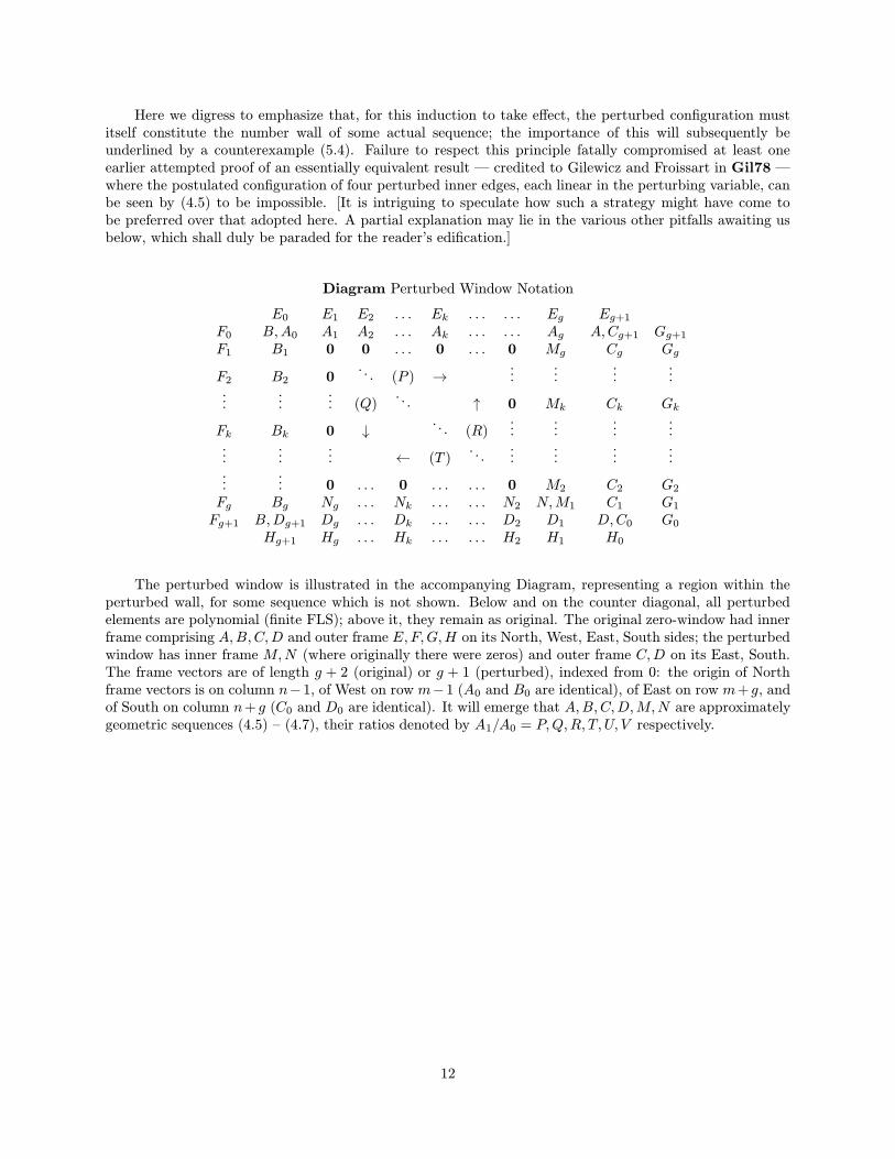
Here we digress to emphasize that, for this induction to take effect, the perturbed configuration mustitself constitute the number wall of some actual sequence; the importance of this will subsequently beunderlined by a counterexample (5.4). Failure to respect this principle fatally compromised at least oneearlier attempted proof of an essentially equivalent result — credited to Gilewicz and Froissart in Gil78 —where the postulated configuration of four perturbed inner edges, each linear in the perturbing variable, canbe seen by (4.5) to be impossible. [It is intriguing to speculate how such a strategy might have come tobe preferred over that adopted here. A partial explanation may lie in the various other pitfalls awaiting usbelow, which shall duly be paraded for the reader’s edification.]

Diagram Perturbed Window Notation

E0 E1 E2 . . . Ek . . . . . . Eg Eg+1F0 B,A0 A1 A2 . . . Ak . . . . . . Ag A,Cg+1 Gg+1F1 B1 0 0 . . . 0 . . . 0 Mg Cg Gg

F2 B2 0. . . (P ) →

......

......

......

... (Q). . . ↑ 0 Mk Ck Gk

Fk Bk 0 ↓ . . . (R)...

......

......

...... ← (T )

. . ....

......

......

... 0 . . . 0 . . . . . . 0 M2 C2 G2Fg Bg Ng . . . Nk . . . . . . N2 N,M1 C1 G1Fg+1 B,Dg+1 Dg . . . Dk . . . . . . D2 D1 D,C0 G0

Hg+1 Hg . . . Hk . . . . . . H2 H1 H0

The perturbed window is illustrated in the accompanying Diagram, representing a region within theperturbed wall, for some sequence which is not shown. Below and on the counter diagonal, all perturbedelements are polynomial (finite FLS); above it, they remain as original. The original zero-window had innerframe comprising A,B,C,D and outer frame E,F,G,H on its North, West, East, South sides; the perturbedwindow has inner frame M,N (where originally there were zeros) and outer frame C,D on its East, South.The frame vectors are of length g + 2 (original) or g + 1 (perturbed), indexed from 0: the origin of Northframe vectors is on column n−1, of West on row m−1 (A0 and B0 are identical), of East on row m+ g, andof South on column n+ g (C0 and D0 are identical). It will emerge that A,B,C,D,M,N are approximatelygeometric sequences (4.5) – (4.7), their ratios denoted by A1/A0 = P,Q,R, T, U, V respectively.

12

Lemma: There are elements U, V such that for 1 ≤ k ≤ g + 1,

Mk = AgUk−g−1, Nk = BgV

k−g−1;

in fact, U = P/X, V = (−)g−1Q/X.(4.5)

Proof: By definition (3.1)

Mg =

∣

∣

∣

∣

∣

∣

∣

Sn+g−1 . . . Sn+g+m−1 + (−)mX...

. . ....

Sn+g−m−1 . . . Sn+g−1

∣

∣

∣

∣

∣

∣

∣

=

∣

∣

∣

∣

∣

∣

∣

Sn+g−2 . . . Sn+g+m−3...

. . ....

Sn+g−m−1 . . . Sn+g−2

∣

∣

∣

∣

∣

∣

∣

X +

∣

∣

∣

∣

∣

∣

∣

Sn+g−1 . . . Sn+g+m−1...

. . ....

Sn+g−m−1 . . . Sn+g−1

∣

∣

∣

∣

∣

∣

∣

,

expanding the determinant;= Ag−1X + 0

in terms of the original wall. Also Mg+1 ≡ Ag , so we can define

U = Mg+1/Mg = Ag/Ag−1X, or U = P/X.

For N, V,Q the only difference is that the determinant is order m+ g − 1; notice that we can use the sameX in both contexts, by (3.8). Finally, for 1 ≤ k ≤ g − 1, by (3.6), Mk+12 =Mk+2Mk, showing that [Mk] isgeometric with ratio U ; similarly for N .

Lemma: There are elements P,Q such that for 0 ≤ k ≤ g + 1,

Ak = A0Pk + O(X), Bk = B0Qk + O(X). (4.6)

Proof: For 0 ≤ k ≤ g, see the end of the proof of (4.5) with P = A1/A0, Q = B1/B0. For k = g + 1, using(3.6) and (4.6) [A is exactly geometric for k < g + 1], we have

Ag+1 = (Ag2 −EgMg)/Ag−1 = A0P g+1 −EgX.

B behaves similarly.It is important to bear in mind that we may always divide by elements of the inner frame or by ratios,

since we know these to be nonzero; indeed the same is true of C and D, even in the perturbed case (4.7). Andwhen multiplying or dividing FLSs (1.1), we need to ascertain that the factors have order sufficiently largeto justify the order claimed for the error in their product: E,F,G,H are always O(1) at worst; A,B,C,Dand P,Q,R, T are O(1) exactly; but U, V are O(1/X).Notice here too that the ‘ratios’ R, T of the approximately geometric outer frames are defined explicitly

by C1/C0, D1/D0, rather than retaining their original values, an apparently insignificant detail which iscentral to the proof: it allows us to get an unexpectedly small and explicit first perturbation term in theexpansions (4.7) of C,D, without which the crucial information carried by the perturbation term in the proofof the central result (4.9) would be swamped by noise of order O(X).

Lemma: There are elements R, T such that for 2 ≤ k ≤ g + 1,

Ck = C0Rk − (R/P )g−k+3Gk−1Xg−k+2 + O(Xg−k+3),

Dk = D0Tk − (−)(g−1)k(T/Q)g−k+3Hk−1Xg−k+2 + O(Xg−k+3).

(4.7)

13

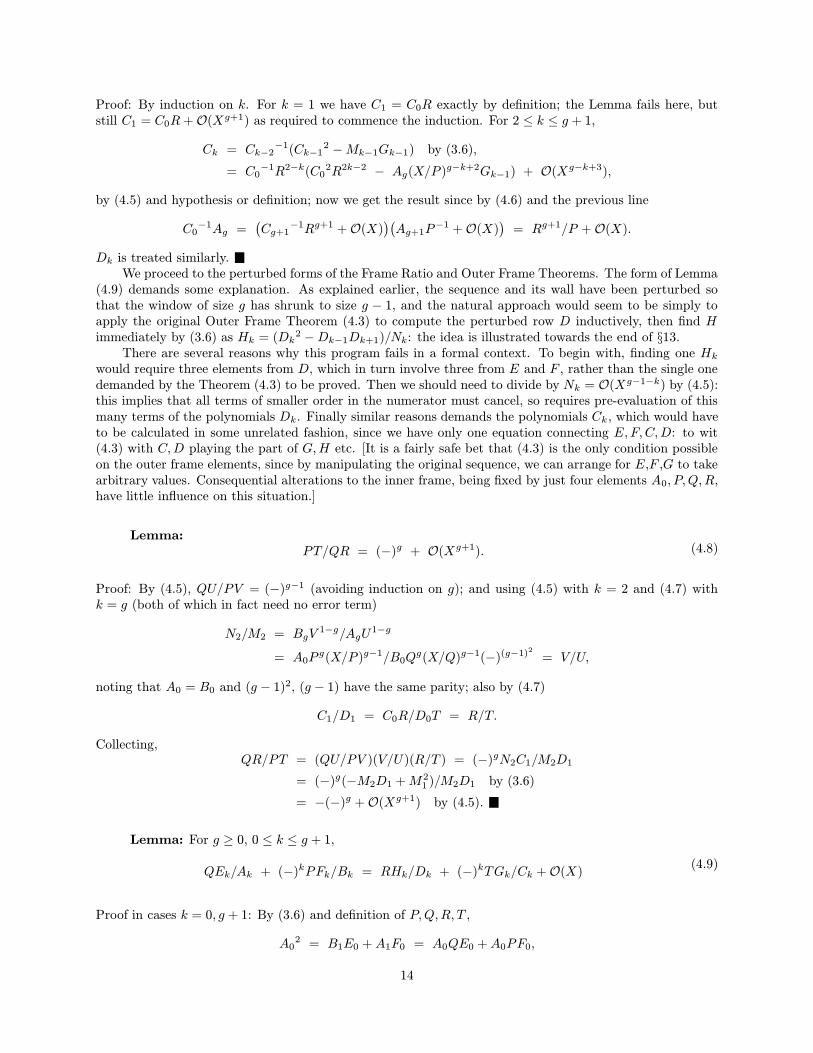
Proof: By induction on k. For k = 1 we have C1 = C0R exactly by definition; the Lemma fails here, butstill C1 = C0R+O(Xg+1) as required to commence the induction. For 2 ≤ k ≤ g + 1,

Ck = Ck−2−1(Ck−1

2 −Mk−1Gk−1) by (3.6),= C0

−1R2−k(C02R2k−2 − Ag(X/P )g−k+2Gk−1) + O(Xg−k+3),

by (4.5) and hypothesis or definition; now we get the result since by (4.6) and the previous line

C0−1Ag =

(

Cg+1−1Rg+1 +O(X)

)(

Ag+1P−1 +O(X)

)

= Rg+1/P +O(X).

Dk is treated similarly.We proceed to the perturbed forms of the Frame Ratio and Outer Frame Theorems. The form of Lemma

(4.9) demands some explanation. As explained earlier, the sequence and its wall have been perturbed sothat the window of size g has shrunk to size g − 1, and the natural approach would seem to be simply toapply the original Outer Frame Theorem (4.3) to compute the perturbed row D inductively, then find Himmediately by (3.6) as Hk = (Dk

2 −Dk−1Dk+1)/Nk: the idea is illustrated towards the end of §13.There are several reasons why this program fails in a formal context. To begin with, finding one Hk

would require three elements from D, which in turn involve three from E and F , rather than the single onedemanded by the Theorem (4.3) to be proved. Then we should need to divide by Nk = O(Xg−1−k) by (4.5):this implies that all terms of smaller order in the numerator must cancel, so requires pre-evaluation of thismany terms of the polynomials Dk. Finally similar reasons demands the polynomials Ck , which would haveto be calculated in some unrelated fashion, since we have only one equation connecting E,F,C,D: to wit(4.3) with C,D playing the part of G,H etc. [It is a fairly safe bet that (4.3) is the only condition possibleon the outer frame elements, since by manipulating the original sequence, we can arrange for E,F ,G to takearbitrary values. Consequential alterations to the inner frame, being fixed by just four elements A0, P,Q,R,have little influence on this situation.]

Lemma:

PT/QR = (−)g + O(Xg+1). (4.8)

Proof: By (4.5), QU/PV = (−)g−1 (avoiding induction on g); and using (4.5) with k = 2 and (4.7) withk = g (both of which in fact need no error term)

N2/M2 = BgV1−g/AgU

1−g

= A0Pg(X/P )g−1/B0Q

g(X/Q)g−1(−)(g−1)2 = V/U,

noting that A0 = B0 and (g − 1)2, (g − 1) have the same parity; also by (4.7)

C1/D1 = C0R/D0T = R/T.

Collecting,QR/PT = (QU/PV )(V/U)(R/T ) = (−)gN2C1/M2D1

= (−)g(−M2D1 +M21 )/M2D1 by (3.6)

= −(−)g +O(Xg+1) by (4.5).

Lemma: For g ≥ 0, 0 ≤ k ≤ g + 1,

QEk/Ak + (−)kPFk/Bk = RHk/Dk + (−)kTGk/Ck +O(X) (4.9)

Proof in cases k = 0, g + 1: By (3.6) and definition of P,Q,R, T ,

A02 = B1E0 +A1F0 = A0QE0 +A0PF0,

14

whence A0−1(QE0 + PF0) = 1; similarly C0

−1(RH0 + TG0) = 1. Also A0 = B0 and C0 = D0, whichproves case k = 0; case k = g + 1 is similar.

Proof in cases 1 ≤ k ≤ g: For g = 0 there are no (further) cases to consider. For g ≥ 1, we assume (4.9),replacing g by g − 1 for the induction; Ck, Dk, Gk, Hk by Mk+1, Nk+1, Ck+1, Dk+1, noticing the shift inorigin caused by the new SE corner; R, T by U , V ; and letting X → 0. Then by inductive hypothesis

Q.Ek/Ak + (−)kP.Fk/Bk= U.Dk+1/Nk+1 + (−)kV.Ck+1/Mk+1= (P/X)(−)(g+1)kBg−1(X/Q)k−gDk+1+ (−)k+g+1(Q/X)Ag−1(X/P )k−gCk+1 + O(X) by (4.5)

= Y + Z +O(Xg−k+2) + O(X), say.

At this point we expand C,D by (4.7) and separate them into main Y , first perturbation Z and residualerror terms. The main terms cancel to order X , as expected:

Y = Xk−g−1(−)g+k+1(

(−)gk+g+1D0Bg−1Q−g(T/Q)kPT + C0Ag−1P−g(R/P )kQR)

= Xk−g−1(−)g+k+1A0C0(

(−)gk+g+1(T/Q)kPT + (R/P )kQR)

since BgQ−g = B0 = A0 = AgP

−g, D0 = C0;

= Xk−g−1(−)g+k+1A0C0(R/P )kQR(−1 + 1) + O(Xg+1)since T/Q = (−)gR/P +O(Xg+1), PT = (−)gQR + O(Xg+1) by (4.8);= O(Xk).

The first perturbation terms incorporate the desired right-hand side:

Z = (−)g+k(

(−)kBg−1PQ−2T g−k+2Hk + Ag−1P−2QRg−k+2Gk)

simplifying — the exponents of X cancel exactly;

= (−)g+k(

(−)k(PT/QR)RHk/Dk + (QR/PT )TGk/Ck)

+ O(X)since AgPR

g−k+1 = Ck + O(X) etc by (4.6) then (4.7) with k = g + 1;= RHk/Dk + (−)kTGk/Ck + O(X) by (4.8).

Collecting Y , Z, etc and checking that the error terms are all O(X) now gives the result.Finally, setting X → 0 in (4.8) and (4.9), we are home and dry in the original wall: (4.1) and (4.3) are

immediate, and (4.2) is a simple consequence of (4.8), (4.6), (4.7). However, notice that this last step is onlypossible because specialization commutes with arithmetic (1.0).

15

5. The Algorithm, Special Cases

By isolating T , Dk and Hk on the left-hand side of the Frame Theorems, we immediately get a comprehensiveand efficient recursion for computing the number-wall by induction on rows m:

Corollary: If m ≤ 0 or Sm−2,n 6= 0 use (3.7); otherwise, determine whether Sm,n, withrespect to the zero-window immediately to the North, lies within:(i) the interior, when by (4.1)

Sm,n = 0 and T = (−)gQR/P ;

(ii) the inner frame, when by (4.2)

Sm,n ≡ Dk = (−)gkBkCk/Ak;

(iii) the outer frame, when by (4.3)

Sm,n ≡ Hk = (Dk/R)(QEk/Ak + (−1)k(PFk/Bk − TCk/Mk)).

(5.1)

Illustrative examples are given later in this section.In principle the original Sylvester recursion (3.6) might be dispensed with, since the Frame Theorems

hold even for g = k = 0; but in practice it is impossible to avoid programming the latter as a special caseanyway, so the saving is only conceptual. [To quote Alf van der Poorten Poo96: In theory, there is nodifference between theory and practice. In practice, it doesn’t quite work that way.]The special case g = k = 1 can be recast in the simplified form:

Corollary: In the notation of the attached figure depicting a portion of the number-wall,for an isolated zero at W we have ED2 +HA2 = FC2 +GB2;

(5.2)

this follows directly by setting W = 0 in the (polynomial) identity:

Lemma: In the notation of the attached figure

ED2 +HA2 −W (EH +AD) = FC2 +GB2 −W (FG+BC). (5.3)

EL A K

F B W C GN D MH

Proof: Suppose W transcendental over the ground domain of [Sn] [strictly, W is some not-identically-vanishing function of transcendental X , such as W = LX where L 6= 0 and X is the perturbation of [Sn] inthe proof of (4.5)]. Expanding LK ·NM = LN ·KM via (3.6) then rearranging,

(A2 −EW )(D2 −HW ) = (B2 − FW )(C2 −GW ),

(BC +AD)(AD −BC) + W (FC2 +GB2 −ED2 −HA2) + W 2(EH − FG) = 0.

Again using (3.6), substituting for BC+AD = W 2, cancelingW and rearranging gives the desired equation.We can now argue, as in the proof of (3.5), that for fixed m this is a polynomial identity in elements ofa sequence [Sn] of distinct transcendentals, so it remains true even when some of the constituent elementssuch as W take zero values. Alternatively, in the spirit of §7, we can examine each possible pattern of zerosindividually, and resolve it by applying (3.8), (4.2) for various g ≤ 3.

16

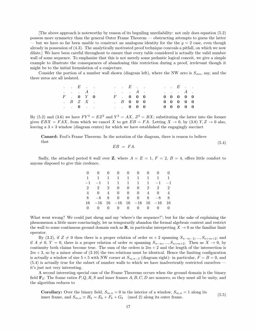
[The above approach is noteworthy by reason of its beguiling unreliability: not only does equation (5.2)possess more symmetry than the general Outer Frame Theorem — obstructing attempts to guess the latter— but we have so far been unable to construct an analogous identity for the the g = 2 case, even thoughalready in possession of (4.3). The analytically motivated proof technique conceals a pitfall, on which we nowdilate.] We have been careful throughout to ensure that every table considered is actually the valid numberwall of some sequence. To emphasize that this is not merely some pedantic logical conceit, we give a simpleexample to illustrate the consequences of abandoning this restriction during a proof, irrelevant though itmight be to the initial formulation of a conjecture.Consider the portion of a number wall shown (diagram left), where the NW zero is Smn, say, and the

three zeros are all isolated.

. . E . .

. . . A .F . 0 Y 0

. B Z X .

. . 0 . .

. . E . .

. . . A .F . 0 0 0

. B 0 0 0

. . 0 0 0

. . E . .

. . . A .0 0 0 0 0

0 0 0 0 0

0 0 0 0 0

By (5.2) and (3.6) we have FY 2 = EZ2 and Y 2 = AX , Z2 = BX ; substituting the latter into the formergives EBX = FAX , from which we cancel X to get EB = FA. Letting X → 0, by (3.8) Y, Z → 0 also,leaving a 3× 3 window (diagram centre) for which we have established the engagingly succinct

Canard: Fool’s Frame Theorem: In the notation of the diagram, there is reason to believethat

EB = FA.(5.4)

Sadly, the attached period 6 wall over Z, where A = E = 1, F = 2, B = 4, offers little comfort toanyone disposed to give this credence.

0 0 0 0 0 0 0 0 01 1 1 1 1 1 1 1 1−1 −1 1 1 1 1 1 −1 −12 2 2 0 0 0 2 2 24 0 4 0 0 0 4 0 48 −8 8 0 0 0 8 −8 816 −16 16 −16 16 −16 16 −16 160 0 0 0 0 0 0 0 0

What went wrong? We could just shrug and say ‘where’s the sequence?’; but for the sake of explaining thephenomenon a little more convincingly, let us temporarily abandon the formal algebraic context and restrictthe wall to some continuous ground domain such as R, in particular interpreting X → 0 as the familiar limitoperator.By (3.2), if Z 6= 0 then there is a proper relation of order m + 2 spanning Sn−m−2, ..., Sn+m+2; and

if A 6= 0, Y = 0, there is a proper relation of order m spanning Sn−m, ..., Sn+m+2. Then as X → 0, bycontinuity both claims become true. The sum of the orders is 2m + 2 and the length of the intersection is2m+ 3, so by a minor abuse of (3.10) the two relations must be identical. Hence the limiting configurationis actually a window of size 5× 5 with NW corner at Sm,n−2 (diagram right): in particular, F = B = 0, and(5.4) is actually true for the subset of number walls to which we have inadvertently restricted ourselves —it’s just not very interesting.A second interesting special case of the Frame Theorems occurs when the ground domain is the binary

field F2: The frame ratios P,Q,R, S and inner frames A,B,C,D are nonzero, so they must all be unity, andthe algorithm reduces to

Corollary: Over the binary field, Sm,n = 0 in the interior of a window, Sm,n = 1 along itsinner frame, and Sm,n ≡ Hk = Ek + Fk +Gk (mod 2) along its outer frame.

(5.5)

17

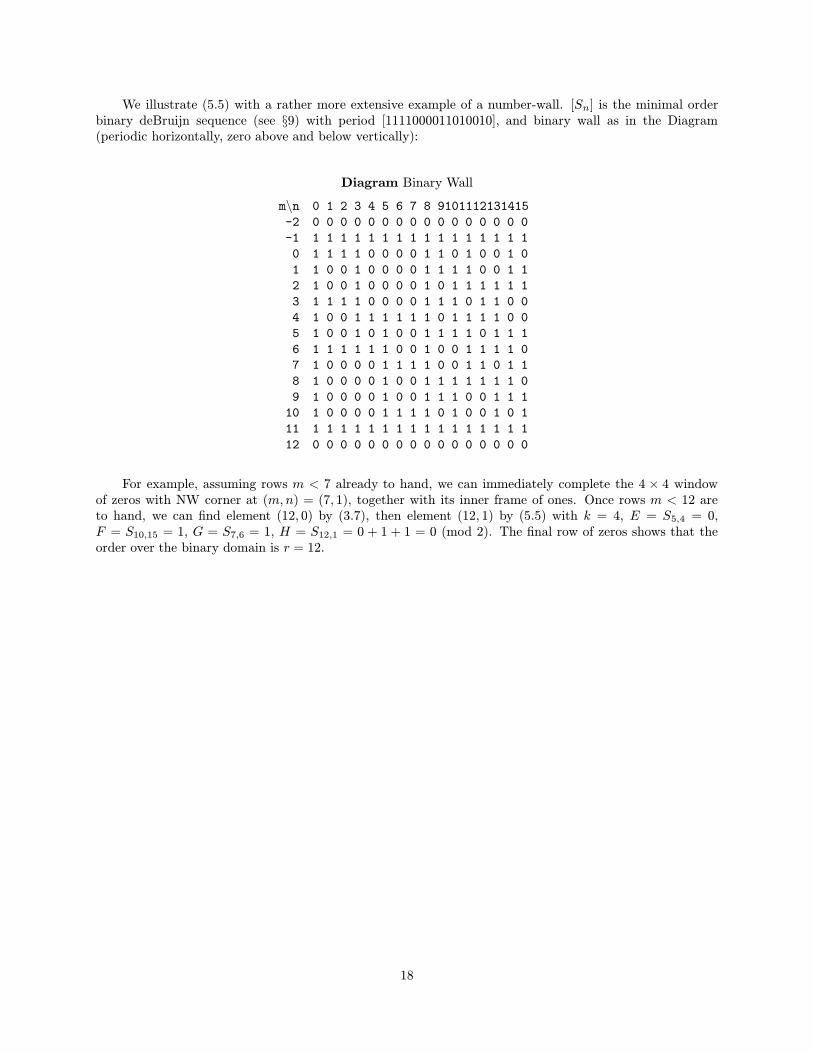
We illustrate (5.5) with a rather more extensive example of a number-wall. [Sn] is the minimal orderbinary deBruijn sequence (see §9) with period [1111000011010010], and binary wall as in the Diagram(periodic horizontally, zero above and below vertically):

Diagram Binary Wall

m\n 0 1 2 3 4 5 6 7 8 9101112131415

-2 0 0 0 0 0 0 0 0 0 0 0 0 0 0 0 0

-1 1 1 1 1 1 1 1 1 1 1 1 1 1 1 1 1

0 1 1 1 1 0 0 0 0 1 1 0 1 0 0 1 0

1 1 0 0 1 0 0 0 0 1 1 1 1 0 0 1 1

2 1 0 0 1 0 0 0 0 1 0 1 1 1 1 1 1

3 1 1 1 1 0 0 0 0 1 1 1 0 1 1 0 0

4 1 0 0 1 1 1 1 1 1 0 1 1 1 1 0 0

5 1 0 0 1 0 1 0 0 1 1 1 1 0 1 1 1

6 1 1 1 1 1 1 0 0 1 0 0 1 1 1 1 0

7 1 0 0 0 0 1 1 1 1 0 0 1 1 0 1 1

8 1 0 0 0 0 1 0 0 1 1 1 1 1 1 1 0

9 1 0 0 0 0 1 0 0 1 1 1 0 0 1 1 1

10 1 0 0 0 0 1 1 1 1 0 1 0 0 1 0 1

11 1 1 1 1 1 1 1 1 1 1 1 1 1 1 1 1

12 0 0 0 0 0 0 0 0 0 0 0 0 0 0 0 0

For example, assuming rows m < 7 already to hand, we can immediately complete the 4 × 4 windowof zeros with NW corner at (m,n) = (7, 1), together with its inner frame of ones. Once rows m < 12 areto hand, we can find element (12, 0) by (3.7), then element (12, 1) by (5.5) with k = 4, E = S5,4 = 0,F = S10,15 = 1, G = S7,6 = 1, H = S12,1 = 0 + 1 + 1 = 0 (mod 2). The final row of zeros shows that theorder over the binary domain is r = 12.

18

If instead we regard [Sn] as defined over the integers, the following wall results. To find element (10, 7)from previous rows we can employ (5.2) with A,B,C,D = 3, 6, 3,−6 and E,F,G = −2, 1, 1, getting

H = (FC2 +GB2 −ED2)/A2 = (1.9 + 1.36 + 2.36)/9 = 13.

To find find our way around the window at (0, 4) with g = 4 demands the full works: happily P = Q = R = 1so T = 1 by (4.1), A = B = C = 1 so D = 1 by (4.2), and we find say element (5, 7) by (4.3) with k = 1 andE,F,G = 0, 1, 3, H = (QE/A− PF/B + TG/C)D/R = 2. The order over the integer domain is r = 13.

Diagram Integer Wall

m\n 0 1 2 3 4 5 6 7 8 9 10 11 12 13 14 15−2 0 0 0 0 0 0 0 0 0 0 0 0 0 0 0 0−1 1 1 1 1 1 1 1 1 1 1 1 1 1 1 1 10 1 1 1 1 0 0 0 0 1 1 0 1 0 0 1 01 1 0 0 1 0 0 0 0 1 1 −1 1 0 0 1 −12 1 0 0 1 0 0 0 0 1 2 1 1 1 1 1 13 1 1 1 1 0 0 0 0 1 3 1 0 −1 −1 0 04 1 2 2 1 1 1 1 1 1 4 1 1 1 1 0 05 1 2 2 −1 0 1 −2 2 −3 5 −3 1 0 −1 1 −16 3 1 3 1 1 1 2 −2 −1 4 4 1 1 1 3 47 5 −4 4 2 0 −1 −3 3 −3 4 −4 −3 −1 2 5 −78 −1 −4 8 4 2 1 6 0 3 1 7 5 7 9 13 69 5 −6 20 0 −8 11 −12 −6 −3 −5 −11 8 −4 −5 23 −710 17 16 50 40 32 25 35 13 −7 −8 23 4 8 13 38 −1111 93 99 93 51 −3 −45 −75 −69 −51 −45 −51 −21 −3 27 69 7512 72 72 72 72 72 72 72 72 72 72 72 72 72 72 72 7213 0 0 0 0 0 0 0 0 0 0 0 0 0 0 0 0

Finally, it is natural to ask is whether a simple recursive algorithm exists for number walls over moregeneral ground rings, in particular over Z/qZ for q an arbitrary natural number. [The obvious approach, tocompute the wall over Z and then reduce (mod q), is less than ideal since the intermediate integers may bevery large.] If q =

∏

k pkek is expressed as a product of prime powers, the residue (mod q) can be computed

easily from residues (mod pe) via the Chinese Remainder Theorem Dav88 §A.5.1, reducing the problem tothe case q = pe. By (3.8), the power of p (or in general, any prime ideal) dividing an element at distance hfrom the frame within a zero-window (mod p) must be at least ph, and one might naıvely hope that perhapsit might be exactly ph (it needn’t); or failing that, the frames might behave in a fashion which generalizesthe situation modulo p, involving the excess over ph near a particular point on the frame. However, it iseasy to construct a wall modulo q = 4 with a large window (mod 2) which is also perfectly square (mod 4),but for which the outer frame sum E + F +G +H varies irregularly between 0 and 2 (mod 4) — stronglysuggesting that the hope is unjustified. [However some progress in this area has been made — see Ree85.]

19

6. General Symmetric Walls

We now need no longer rely on the determinant approach (3.1) to define the number-wall, but may generateit instead by placing an arbitrary pair of sequences [Tn], [Sn] on rows m = −1, 0 — subject to zero-windows(3.8), and supplemented where necessary by consistent frame data around such windows — then employingframe recursion (5.1) for m > 0, and by reflection for m < −1. The unexpected square-tiling symmetryof the new definition is noteworthy: Since neither m nor n appears explicitly, we have invariance under2-D translations; furthermore, despite an apparent asymmetry of (3.1) between m and n, (4.1) – (4.3) areinvariant under reflection in diagonals of the window, and under half-turn about its centre. [This last israther less mysterious when viewed in the context of Pade tables §11, where it arises directly from the factthat the reciprocal transpose of the Pade table for F (X) is the table for 1/F (X).] To distinguish the newwall from the special number wall (SNW) of (3.1) etc, we refer to it as a general symmetric wall (GSW). [Itmust be admitted that at the moment this construction, as was memorably observed of an entirely differentsubject, fills a much-needed gap.]The elements of a GSW are plainly rational functions in the elements from which they are generated;

and it seems reasonable to suppose that they should possess some explicit characterization, analogous to(3.1) defining the SNW. Such an expression would undoubtedly be immediately useful (see below), but atpresent we have in lieu only the following partial result, initially communicated to us by Jim Propp as acorollary of a more general combinatorial expression in Rob86.

Theorem: For m ≥ 1, the general element Sm,n of a GSW constructed (via (3.7)) fromsequences of variables S−1,n = Un and S0,n = Vn is of the form Sm,n = Wm,n/Zm,n, whereWm,n is an irreducible polynomial of total degree (at most) 2(m

2 −m+ 1) in the assortedvariables, and Zm,n is (a factor of) the degree m

2 + (m− 1)2 monomial

Zm,n =

k=m−1∏

k=1−m

Un+km−|k|Vn+k

m−1−|k|.

(6.1)

For m < 0, immediately by symmetry

Sm,n(. . . , Uk, . . . , Vk, . . .) = S−1−m,n(. . . , Vk, . . . , Uk, . . .).

Proof: Notice that in the setting of a GSW, both m and n subscripts may be arbitrarily translated; sowithout loss of generality, we may represent an arbitrary element Sm,n by S4,4. By (3.6),

S44 = (S234 − S33S35)/S24. (6.2)

Also, substituting for the S3,j ,

S44 =(

S224 − S23S25)2/S214 − (S223 − S22S24)(S225 − S24S26)/S13S15)

/S24.

Most of the terms in the numerator of the right-hand side above have a factor S24, the exceptions simplifyingto

−S23S225(S214 − S13S15)/S13S214S15S24 = −S04S23S225S24/S13S214S15S24using (3.6); so S24 cancels completely from the denominator, giving

S44 =S13S15S

324 − 2S13S15S23S24S25 − S214S22S24S26 + S214S223S26 + S214S22S225 − S04S223S225

S13S214S15. (6.3)

We proceed by induction on m: elementary computation as above establishes (6.1) for m = 1, 2. Form > 2, translating (6.2) and (6.3) from S4,4 to Sm,n, we see Sm,n must be of the form (6.1), possibly dividedby some factor of the HCF of Wm−2,n and W

2m−3,nWm−3,n−1Wm−3,n+1. However, we show below that Wi,j

20

is an irreducible polynomial in the Uk and Vk , so this HCF is unity, and Sm,n is also of the form (6.1) asrequired.To establish the irreducibility of Wm,n, we consider first the special number wall of a transcendental

sequence [Vk], i.e. Uk = 1 for all k. Notice that any factor of a homogeneous polynomial must also behomogeneous, since the product of two polynomials with minimum total degree a, c and maximum b, d resp.necessarily contains terms of degrees a+ c and b+ d. Fixing say n = m, by (3.1)

Sm,m =

∣

∣

∣

∣

∣

∣

Vm . . . V2m.... . .

...V0 . . . Vm

∣

∣

∣

∣

∣

∣

.

V2m has cofactor Sm−1,m−1, which by assumption is irreducible. So if Sm,m factorizes properly, it has alinear factor containing V2m; and the other factor must equal Sm−1,m−1, which does not contain Vm

m. Sotheir product does not contain Vm

m+1, and cannot be Sm,m: thus in the special number wall of a sequenceof distinct transcendentals, Sm,m and by translation Sm,n is an irreducible polynomial.

Now consider the GSW. IfWm,n factorizes properly, it has a factor containing no Vk elements (otherwisewe could specialize to a factorization for the special wall above). By an easy induction using (3.6), Wm,ncontains just one term which is a multiple of Vn

m+1: specifically, Zm,nVnm+1/Umn . So any factor can only

be a monomial which (partially) cancels with the denominator as given above, and what remains of thenumerator is irreducible.A more refined induction ought to show that not even monomial cancellation can occur above; hence

that the polynomial degrees and the form of Zm,n given in (6.1) are exact, and indeed that the total degreeof Wm,n in the Uk, Vk separately is uniformly m(m − 1), m(m − 1) + 2 resp. Moreover we conjecture thatthe sum of the absolute values of the coefficients of Wm,n is 2

m(m+1)/2. This last quantity — essentially thenumber of terms in the m-th row of a polynomial GSW — is uncomfortably large: for example, W4,n is apolynomial of about 30, 000 terms, each of degree 26.

A referee has made the point that we have inadvertently introduced not one but two generalizationshere. Given sequences [Tn], [Sn] over the ground domain, firstly we generate the ‘numerical’ GSW Sm,n viarecursion (5.1); secondly we substitute them for [Un], [Vn] in the formal GSW (6.1). [It is assumed both[Tn], [Sn] everywhere nonzero, ensuring both that (3.8) holds initially — without which no (5.1)) — and thatthe denominators Zm,n are nonzero in (6.1).] Now, are the two walls equal? If we had an explicit expressionfor the GSW element, we might consider adapting the Frame Theorem proof to incorporate it. Failing that,we can at least observe that they are surely equal if either wall is everywhere nonzero, since algorithms (3.7)and (5.1) are then equivalent; and again, they are equal if [Tn], [Sn] happen to be a pair of adjacent rows (orindeed columns) from some pukka SNW, by the existing Frame Theorem.Now any given GSW element depends on only a finite subset of [Tn], [Sn]. We might therefore seek to

show that every finite region of the GSW may be embedded in some SNW, generated by some sequence [Rn]say (dependent on the region). [The region may be taken to be a (square) diamond, with base on the row[Tn] and apices at some target element and its reflection in the base]. In specific instances, this embedding isstraightforward to verify: the equations for [Rn] turn out to be linear in [Tn], [Sn], and it appears sufficientto consider [Rn] of period at most thrice the diameter. However, a general proof is complicated by the factthat any fixed scheme of equations may be rendered singular by some zero within the region, in spite of thefact that in practice such zero-windows make a specific problem easier to solve.We turn to another question posed by Propp, the statement and solution of which exemplify the geo-

metric nature of the number wall. It concerns the extent to which the frame rules might be in some covertfashion local, in the sense that the value of an element is independent on those outside some bounded neigh-borhood. Specifically he asks: given arbitrarily large k, do there exist two distinct walls with k (or more,but only finitely many) consecutive rows in common? Such questions as what ground domain is specified,whether horizontal and/or vertical translations are to be regarded as differences in this context, and whetherthe wall is special, can be postponed; we shall see that the answer turns out to satisfy the most stringent ofsuch conditions.Consider an arbitrary relation J of order r with leading and trailing coefficients equal to unity, with

[Sn] satisfying S1 = . . . = Sr−1 = 0 and Sr = 1 (the so-called impulse response sequence or IRS), and having

21

period q; then define

Tn ={

Sn if r ≤ n ≤ q;0 otherwise.

Then the wall for T is easily seen to be of form diagrammed, where Zg denotes a g × g window (with innerframe unity), R denotes the (r + 1) × (q − r + 1) rectangular region comprising one period of the wall for[Sn] but excluding its initial Zr−1, and R

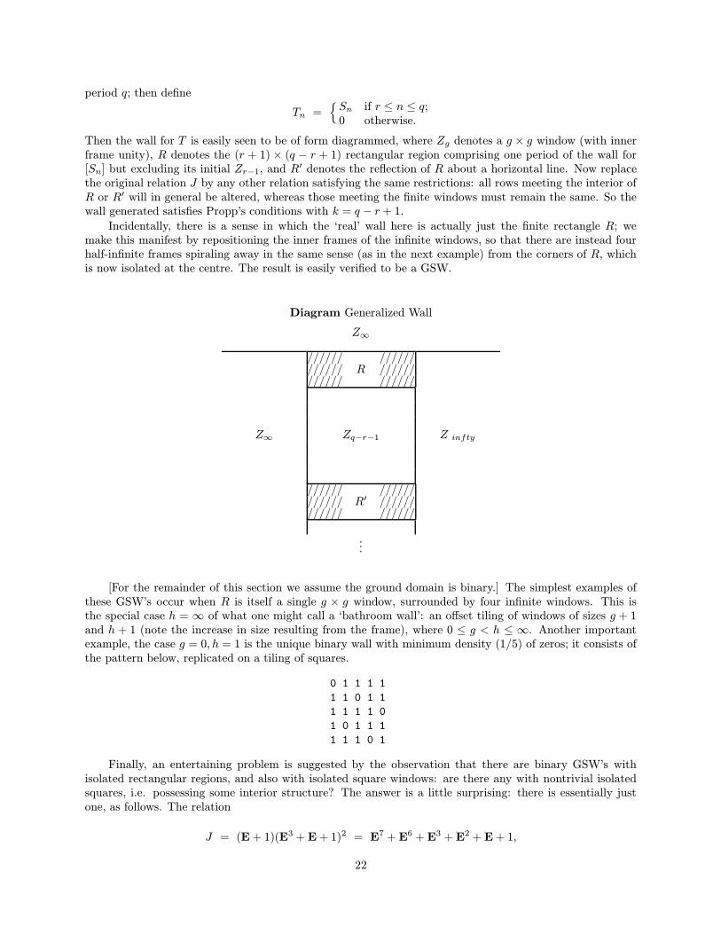
′ denotes the reflection of R about a horizontal line. Now replacethe original relation J by any other relation satisfying the same restrictions: all rows meeting the interior ofR or R′ will in general be altered, whereas those meeting the finite windows must remain the same. So thewall generated satisfies Propp’s conditions with k = q − r + 1.Incidentally, there is a sense in which the ‘real’ wall here is actually just the finite rectangle R; we

make this manifest by repositioning the inner frames of the infinite windows, so that there are instead fourhalf-infinite frames spiraling away in the same sense (as in the next example) from the corners of R, whichis now isolated at the centre. The result is easily verified to be a GSW.

Diagram Generalized Wall

Z∞

////// //////////// R //////////// //////

Z∞ Zq−r−1 Z infty

////// //////////// R′ //////////// //////

...

[For the remainder of this section we assume the ground domain is binary.] The simplest examples ofthese GSW’s occur when R is itself a single g × g window, surrounded by four infinite windows. This isthe special case h = ∞ of what one might call a ‘bathroom wall’: an offset tiling of windows of sizes g + 1and h + 1 (note the increase in size resulting from the frame), where 0 ≤ g < h ≤ ∞. Another importantexample, the case g = 0, h = 1 is the unique binary wall with minimum density (1/5) of zeros; it consists ofthe pattern below, replicated on a tiling of squares.

0 1 1 1 1

1 1 0 1 1

1 1 1 1 0

1 0 1 1 1

1 1 1 0 1

Finally, an entertaining problem is suggested by the observation that there are binary GSW’s withisolated rectangular regions, and also with isolated square windows: are there any with nontrivial isolatedsquares, i.e. possessing some interior structure? The answer is a little surprising: there is essentially justone, as follows. The relation

J = (E+ 1)(E3 +E+ 1)2 = E7 +E6 +E3 +E2 +E+ 1,

22

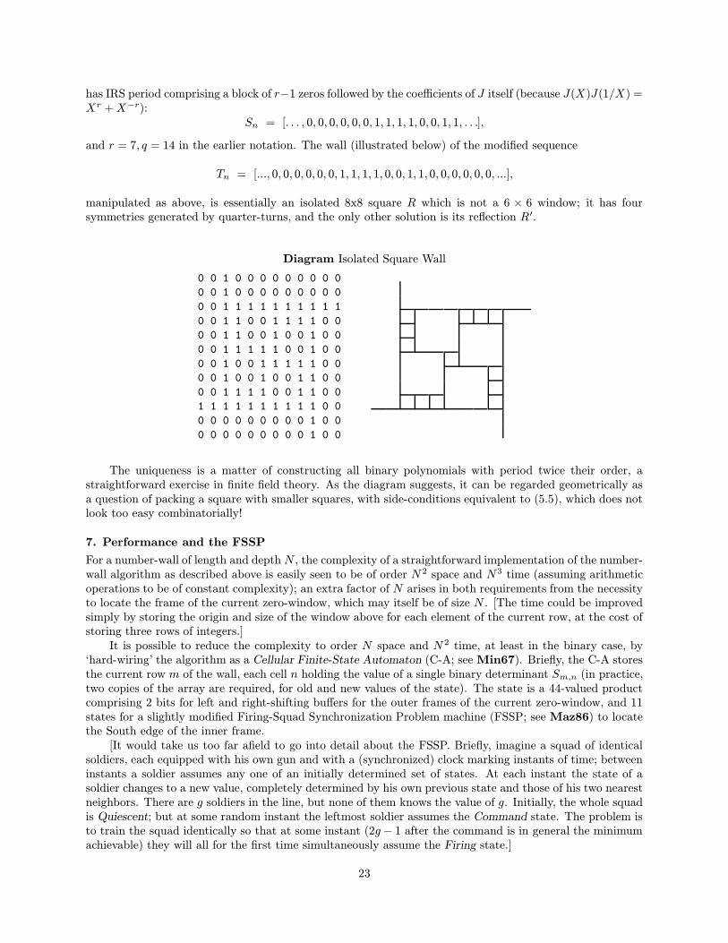
has IRS period comprising a block of r−1 zeros followed by the coefficients of J itself (because J(X)J(1/X) =Xr +X−r):

Sn = [. . . , 0, 0, 0, 0, 0, 0, 1, 1, 1, 1, 0, 0, 1, 1, . . .],

and r = 7, q = 14 in the earlier notation. The wall (illustrated below) of the modified sequence

Tn = [..., 0, 0, 0, 0, 0, 0, 1, 1, 1, 1, 0, 0, 1, 1, 0, 0, 0, 0, 0, 0, ...],

manipulated as above, is essentially an isolated 8x8 square R which is not a 6 × 6 window; it has foursymmetries generated by quarter-turns, and the only other solution is its reflection R′.

Diagram Isolated Square Wall

0 0 1 0 0 0 0 0 0 0 0 0

0 0 1 0 0 0 0 0 0 0 0 0

0 0 1 1 1 1 1 1 1 1 1 1

0 0 1 1 0 0 1 1 1 1 0 0

0 0 1 1 0 0 1 0 0 1 0 0

0 0 1 1 1 1 1 0 0 1 0 0

0 0 1 0 0 1 1 1 1 1 0 0

0 0 1 0 0 1 0 0 1 1 0 0

0 0 1 1 1 1 0 0 1 1 0 0

1 1 1 1 1 1 1 1 1 1 0 0

0 0 0 0 0 0 0 0 0 1 0 0

0 0 0 0 0 0 0 0 0 1 0 0

The uniqueness is a matter of constructing all binary polynomials with period twice their order, astraightforward exercise in finite field theory. As the diagram suggests, it can be regarded geometrically asa question of packing a square with smaller squares, with side-conditions equivalent to (5.5), which does notlook too easy combinatorially!

7. Performance and the FSSP

For a number-wall of length and depth N , the complexity of a straightforward implementation of the number-wall algorithm as described above is easily seen to be of order N 2 space and N3 time (assuming arithmeticoperations to be of constant complexity); an extra factor of N arises in both requirements from the necessityto locate the frame of the current zero-window, which may itself be of size N . [The time could be improvedsimply by storing the origin and size of the window above for each element of the current row, at the cost ofstoring three rows of integers.]It is possible to reduce the complexity to order N space and N 2 time, at least in the binary case, by

‘hard-wiring’ the algorithm as a Cellular Finite-State Automaton (C-A; seeMin67). Briefly, the C-A storesthe current row m of the wall, each cell n holding the value of a single binary determinant Sm,n (in practice,two copies of the array are required, for old and new values of the state). The state is a 44-valued productcomprising 2 bits for left and right-shifting buffers for the outer frames of the current zero-window, and 11states for a slightly modified Firing-Squad Synchronization Problem machine (FSSP; seeMaz86) to locatethe South edge of the inner frame.[It would take us too far afield to go into detail about the FSSP. Briefly, imagine a squad of identical

soldiers, each equipped with his own gun and with a (synchronized) clock marking instants of time; betweeninstants a soldier assumes any one of an initially determined set of states. At each instant the state of asoldier changes to a new value, completely determined by his own previous state and those of his two nearestneighbors. There are g soldiers in the line, but none of them knows the value of g. Initially, the whole squadis Quiescent; but at some random instant the leftmost soldier assumes the Command state. The problem isto train the squad identically so that at some instant (2g− 1 after the command is in general the minimumachievable) they will all for the first time simultaneously assume the Firing state.]

23

In the notation of the Frame Theorems (§4 figure), each cell picks up E from the North of the window,then shifts it rightward until it hits the East frame, where G is added in, after which E+G is sent leftward. Inthe meantime F from the West is shifted rightward until the two collide on the South frame, where they areadded to give H . The FSSP is started by commands in both North corners of the window simultaneously, sothat it fires after g steps rather than 2g; sadly, this means we cannot employ Mazoyer’s beautiful asymmetric6-state solutionMaz87, although we could use Balzer’s symmetric 8-state solution to reduce the state totalto 40. The transition table for the binary C-A is only 85 Kbyte, and it is quite stunningly fast: a single 3-Darray lookup for each determinant computed. Because of the localization of the data, on a massively parallelmachine the complexity improves to order N time and space.The C-A method can in principle be generalized to ground field Zp, but implementation seems to demand

on the order of p5 states, so is unlikely to be feasible for p > 3. A more practical approach is to retain theFSSP synchronization and the technique of shifting frame values right or left till they bounce off the frameof the window, but abandon any attempt to do arithmetic in the control structure: the values of the frameelements are simply shifted separately, each inner or outer edge having its own row of shifting buffers (A,Eneed two each, but their rightward buffers can be shared with B,F ). The arithmetic for the South frame isall performed explicitly when the FSSP fires. This requires around ten one-dimensional arrays to implement,and retains the order N space and N 2 time complexity of the C-A, as well as its potential for parallelization.The Frame algorithm (5.1), including the binary C-A variant, has been implemented in C-language as

part of a sophisticated application program running on a Sun SPARC workstation, incorporating a graphicalfront-end allowing large segments (up to one million elements) of a number-wall to be viewed in color-coding.At a more modest level, there is available a pedagogic Maple implementation of most of the algorithmsdescribed here, designed for the examples shown here.

8. Interpolation and Vandermonde Matrices

In the next three sections we turn to a distinct but closely related problem, which receives surprisingly littleattention in standard texts: the efficient computation of the explicit form of Sn for an LFSR sequence [Sn]from its relation and/or from (a sufficiency of) its terms. The first two sections summarize and dilate uponstandard material required for the third.We denote by σi(X1, . . . , Xr) the elementary symmetric function of degree i on r variables Xi, and

recall the well-known

Lemma: The polynomial equation with roots X = X1, . . . , Xr

J(X) =∏

k

(X −Xk) =∑

i

JiXi

has coefficients given by Ji = (−)r−iσr−i((X1, . . . , Xr)).

(8.1)

For development and analysis of algorithmic efficiency, we need to make the point that all the ‘defective’symmetric functions σi(. . . , X 6=k, . . .) — that is, on r−1 variables excludingXk — can be computed efficientlyin order r2 time by first employing and then reversing the usual inductive algorithm:

Algorithm: Initially for i = 0, k = 0, 1, . . . , r set σ0(X1, . . . , Xk) = 1;for k = 0, i = 1, . . . , r set σi() = 0;for k = 1, 2, . . . , r set

σ0(X1, . . . , Xk) = 1,

σi+1(X1, . . . , Xk) = σi+1(X1, . . . , Xk−1) +Xkσi(X1, . . . , Xk−1);

then for k = 1, 2, . . . , r set

σ0(. . . , X 6=k, . . .) = 1,

σi+1(. . . , X 6=k, . . .) = σi+1(X1, . . . , Xr)−Xkσi(. . . , X 6=k, . . .).

(8.2)

24

From now on we shall assume that the [Xi] are distinct, that is either they are transcendental orXi 6= Xjfor 1 ≤ (i, j) ≤ r. We require some properties of the (fairly) well-known Vandermonde matrixM , defined by

Definition:

Mij = (Xj)i. (8.3)

Its determinant is given by

Theorem:

|Mij | =∏

k

∏

l<k

(Xk −Xl), (8.4)

and its matrix inverse by N ·M = I where

Theorem:

Nji =(−)i−1σr−i(. . . , X 6=j , . . .)∏

k 6=j(Xk −Xj). (8.5)

Proof: As any undergraduate used to know, by subtracting column l from k, the determinant divides by(Xk −Xl); and by inspecting the diagonal term, the remaining constant factor is unity. The inverse (hintedat darkly in Knu81 §1.2.3 Ex. 40 and in Ait62 §49) is more or less immediate by (8.1) with Xj replacingX and omitted from the roots:

(N ·M)ij =∑

k

NikMkj

=

∑

k(−)i−1σr−k(. . . , X 6=i, . . .)(Xj)k∏

k 6=j(Xk −Xj)

=∏

k 6=i

(Xk −Xj)/∏

k 6=j

(Xk −Xj) = Iij

where Iij denotes the Kronecker delta. [The commutation M ·N = I is considerably less obvious!]By (8.5) we can explicitly solve the simultaneous linear equations K ·M = S arising in fitting a linear

combination of given exponentials, since K = S ·N :

Corollary:

Si =∑

j

KjXji

if and only if

Kj =

∑

i Si(−)iσr−i−1(. . . , X 6=j , . . .)∏

k 6=j(Xk −Xj).

(8.6)

Returning to our illustration, suppose we have established as in §2 or §3 that S = [0, 0, 0, 1, . . .] is anLFSR sequence with relation which turns out to factor as J(E) = (E − 7)(E − 5)(E − 3)(E − 1); so itsroots are [X1, X2, X3, X4] = [7, 5, 3, 1] and the difference products [(X2 −X1)(X3 −X1)(X4 −X1), . . .] =[−48,+16,−16,+48]. Computing the elementary and defective symmetric functions via (8.2) gives

i\k 0 1 2 3 40 1 1 1 1 11 0 7 12 15 162 0 0 35 71 863 0 0 0 105 1764 0 0 0 0 105

i\k 1 2 3 40 1 1 1 11 9 11 13 152 23 31 47 713 15 21 35 105

.

25

Substituting all these into (8.6) gives [K1,K2,K3,K4] = [+1,−3,+3,−1]/48, whence the explicit form is

Sn = (1 · 7n − 3 · 5n + 3 · 3n − 1 · 1n)/48.

Finally, a surprising application of the Vandermonde determinant gives a formula for the number-wallof an LFSR sequence:

Theorem: If Sn =∑

iKiXin, then in its number-wall Sm,n =

∑

j BjYjn−m, where Yj =

∏

kXk is the product of any m+ 1 of the Xi, and

Bj =∏

k

Kk ·∏

k

∏

l6=k

(Xk −Xl).

Here j indexes subsets of size m+ 1 from {1, . . . , r}, the indices k, l being restricted to thisj-th subset.

(8.7)

Proof: Express the m = r − 1 case as product of two Vandermonde determinants:

Sm,n = |Sn+i−j | =∣

∣

∑

k

KkXkn+i−j

∣

∣ = |KjXj i| · |Xin−j |.

For 0 ≤ m ≤ r−1 every term of the expanded determinant defines a unique subset of m+1 from r; collectingtogether all the terms with the same subset, we see that we must sum the VDM product over all such subsets.[This is best worked through on a small example: the sign of the result requires care.]We shall later require an explicit formula for the number-wall for the binomial coefficients along the

diagonals of the Pascal triangle, discussed in greater depth in the next section (9.4):

Theorem: The number-wall for Sn =(

nr−1

)

is given by

Sm,n =

k=m∏

k=0

(

n− kr − 1−m

)

/

(

r − 1−m+ kr − 1−m

)

if −1 ≤ m ≤ r − 1,

0 otherwise.

(8.8)

Proof: Assume for the moment that Sm,n is defined by the above expression. Evidently S−1,n = 1 andS0,n =

(

nr−1

)

as required. If we ignore the sole r − 2 × r − 2 zero-window at the origin (which turns out togive no trouble), we need only show that (3.6) is satisfied to clinch the result.For −1 ≤ m ≤ r − 1 the expression may be recast, more explicitly if less elegantly, as

Sm,n =

k=r−1∏

k=0

(n− kk + 1

)min(k + 1, r − 1− k, m+ 1, r − 1−m).

By somewhat tedious comparison of the k-th exponents in pairs of elements of this form, it can be shownthat, for 0 ≤ m < r/2− 1 at least,

Sm−1,n/Sm,n = (r − 1−m) . . . (m+ 1)/(n−m)...(n− r +m+ 2),Sm+1,n/Sm,n = (n−m− 1) . . . (n− r +m+ 3)/(r − 2−m)...(m+ 2),Sm,n−1/Sm,n = (n− r +m+ 1) . . . (n− r + 1)/(n)...(n− r),Sm,n+1/Sm,n = (n+ 1) . . . (n− r + 1)/(n− r +m+ 2)...(n− r + 2);

whence easilySm−1,nSm+1,n/S

2m,n = (m+ 1)(r −m− 1)/(n−m)(n− r +m+ 2),

Sm,n−1Sm,n+1/S2m,n = (n− r + 1)(n+ 1)/(n−m)(n− r +m+ 2);

26

so(Sm−1,nSm+1,n + Sm,n−1Sm,n+1)/S

2m,n = 1,

and (3.6) is satisfied.For r/2 − 1 ≤ m < r, notice that the recast expression is symmetric under m → r − 2 −m; therefore

the entire wall is symmetric about its horizontal midline, and (3.6), also symmetric, is satisfied here too.We are (almost) in a position to characterize the rows of an LFSR wall:

Corollary: If [Sn] is an LFSR sequence of order r, then for each m [Sm,n] is an LFSR

sequence of order at least max(0, 1 + (m+ 1)(r − 1−m)) and at most(

r

m+ 1

)

.(8.9)

Proof: the upper bound results from assuming all the Yj distinct in (8.7), and applying (2.2) conversely; thelower bound from assuming that the Yj coincide (say with unity), then observing that (3.10) in the nonzeroregion is the product of m+1 polynomials of degree r− 1−m in n; by expanding the Toeplitz determinant,the addition of lower-degree terms to K(n) and the geometric factor Y n = Xmn make no difference to theorder.Any coincidence between two Yj corresponding to distinct choices of Xi in (8.7) serves merely to reduce

the order of the row by the smaller of their contributions. The general case of multiple roots Xi in therelation itself is more involved: it would divert us too far to attempt to analyse it here, and we contentourselves with a plausible assertion: the order of any row of the wall of an LFSR sequence, satisfying a givenrelation with possibly multiple roots, cannot increase if the relation is massaged so as to cause coincidencesadditional to those already present.The computation of the actual relation satisfied by a given row of the wall generated by a given relation

is an interesting exercise in symmetric functions, which again shall not detain us here.

9. Difference Tables

Extrapolation of a sequence is a common requirement, arising in numerical computation, recreational prob-lems, critical-point estimation and cryptographic contexts. The familiar Difference Table, see for exampleFro85 §14, is defined by the recursion

Definition:

T0,n = Sn;

Tm,n = (E− 1)mSn = ∆mSn = Tm−1,n+1 − Tm−1,n for m > 0;(9.1)

it has the property that Tm,n vanishes for all m > r just when Sn equals a polynomial in n of degree r. Byextending the region of zeros with n then reversing the direction of the recursion with m, we can efficientlyextrapolate such a sequence to greater n. Further, the explicit form of the polynomial may be recovered viaNewton’s forward difference formula, subject to the caveat below:

Theorem: If the polynomial sequence [Sn] has difference table [Ti,j ] then

Sn =∑

i

Ti,0

(

n

i

)

. (9.2)

Similarly if [Sn] is LFSR of order r, then by (3.3) its wall vanishes for m > r. Since by (2.2) apolynomial sequence of degree r is a (special case of a) LFSR sequence of degree r+1, the same use may bemade of the number-wall to give a generalized extrapolation algorithm, albeit requiring an extra term anda rather more complicated computation of the explicit form. This application is described in an elementaryfashion in Slo95 §1 and Con96 §3, employing an ingenious notation unhappily compromised by a clutch ofdemoralizing misprints.

27

A difficulty with interpreting (2.2) for finite ground characteristic p is that the Little Fermat Theoremnp = n (mod p) effectively prevents the degree of ‘naıve’ polynomials based on powers nj from exceedingp− 1. A straightforward solution to the difficulty is suggested by (9.2): to base our polynomials on binomialcoefficients

(

nj

)

instead. This falls over in a similar fashion if we attempt the usual

Definition:(

n

j

)

=∏

0≤i<j

(n− i)/(i+ 1). (9.3)

But as it happens, the computation of binomial coefficients for characteristic p is the stuff of numerousrecreational articles and student projects. Write l = pk. Decomposing the difference table for

(

nl−1

)

(which

is just the IRS of El − 1) into p2 blocks of edge l/p, observing that each block is a multiple of the table for(

npl/p−1

)

, and that the blocks themselves satisfy the Pascal triangle recursion (2.3), by induction on k we get

the pretty result (ascribed to Lucas in the survey article Gra96):

Theorem:

(

n

m

)

≡

∏

i

(

nimi

)

(mod p) if n ≥ 0, m ≥ 0,

(−)−n+m−1(−n+m− 1

m

)

if n < 0, m ≥ 0,0 if m < 0,

(9.4)

where ni and mi denote the digits of n and m written to base p; the later parts of the right-hand side areelementary.This costs order logn time; the terms on the right-hand side can be computed easily via (2.3) as a table

of p2 entries. It also demonstrates that the binomial coefficient is mathematically defined within the domain,allowing us to apply all the usual machinery of difference calculus within the domain as well. A simpleillustration of the situation is [Sn] = [0, 0, 0, 1, 0, 0, 0, 1, . . .] for n = 0, 1, 2, . . ., with relation Sn+4 − Sn = 0whose quadruple root over the binary domain is X = 1. By LFT, no naıve binary polynomial can haveperiod > 2; but as required

[

(

n

3

)

] = [0, 0, 0, 1, 4, 10, 20, 35, ...] ≡ [Sn] (mod 2)

Sequences with period a power of the characteristic have a useful property:

Lemma: If [Sn] has period l = pk then

(El − 1)[Sn] = (E− 1)l[Sn] = [On],(9.6)

since(

lj

)

= 0 except when j = 0, l, using (9.4). So by (2.2), Sn is a polynomial (in the binomial sense) of

degree r, where l/p < r ≤ l (unless the period is l/p or smaller). By (9.1), we can employ a difference tablerather than a number wall to compute its order. Moreover, by (9.6) in reverse, we can difference pi times inthe same time as differencing once: so initially setting i = k and progressively reducing i as the period ofthe current row m decreases, we can compute the order in kp rows instead of l, giving about order lp time.We illustrate the method with a Maple program:

Algorithm:

orderSpk := proc (S, p, k)

local T, dT, m, j, l;

l := p∧k; m := 0; T := S;while l > 1 do

dT := [seq((T[j+l/p mod l +1] - T[j+1]) mod p, j = 0..l-1)];

if sum(dT[j+1], j = 0..l-1) = 0

then l := l/p else m := m + l/p; T := dT fi od;

m + min(1, T[1]) end;

(9.7)

28

An application of the preceding theory occurs in the study of deBruijn sequences, which are definedtraditionally over a finite set of size q as k-distributed (every k-tuple occurring with the same frequency),and having minimum period qk. In the case where the set is actually a finite field, the extra structure allowsus to define and compute the order of the sequence qua LFSR sequence over that domain; now the methodoutline above can be employed to substantially reduce the time (by the traditional factor of l/ log l). Inan investigation such as Bla96, Cha82 where the computation of the order is the inner loop of a lengthycombinatorial search, such a reduction is crucial. [In fact Bla96 employed a more involved formulation ofpolynomials, basing the computation of the order on a modified Fast Fourier Transform.]As a numerical example, we compute the order of the deBruijn sequence with q = p = 2, k = 5

and order r = 21 over F2 (but 25 over Z). [It is essentially unique, modulo reflection and (independent)complementation of the first or last half.] T denotes the current m-th difference of S, l the currently detectedperiod; when the l/p-th difference of T would be zero, the period is reduced instead.

l m dT = 0? T32 0 N 1111100100000101001110101100011032 16 Y 1100001111000011110000111100001116 16 Y 11000011110000118 16 N 11000011110000118 20 Y 111111114 20 Y 11112 20 Y 111 20 N 10 21

For the deBruijn sequence with q = p = 2, k = 4 at the end of §6, we find from the full difference table (notshown) that Ti,0 = 1 only for i = 0, 4, 10, 11; therefore an explicit ‘binomial’ expression for the n-th term is

Sn = 1 +

(

n

4

)

+

(

n

10

)

+

(

n

11

)

.

Finally, we touch on a rather curious interaction between difference tables and number walls, whichcomes to light when we try to establish exactly what effect a simple transformation of the sequence has onits wall. For instance, a little thought suggests that term-by-term addition of a low-order LFSR sequenceto [Sn] will only have a (literally) marginal effect on any large windows, causing their frames to shift by atmost the order added. However, our only explicit progress in this direction is the

Theorem: The wall for 1+Sn is just the wall for Sn itself added to the wall for −∆2Sn−1shifted down by one row. That is,

Let Rn = 1 + Sn, Tn = −Sn+1 + 2.Sn − Sn−1; then Rm,n = Sm,n + Tm−1,n(9.8)

Proof: Rather than attempt a formal but notationally impenetrable proof for the general case, we illustrateit by the case m = n = 3. Starting from the determinant definition (3.1), R33 =

∣

∣

∣

∣

∣

∣

∣

1 + S3 1 + S4 1 + S5 1 + S61 + S2 1 + S3 1 + S4 1 + S51 + S1 1 + S2 1 + S3 1 + S41 + S0 1 + S1 1 + S2 1 + S3

∣

∣

∣

∣

∣

∣

∣

;

expanding each by column in turn, and noticing that any determinant with two or more equal columns ofones must be zero, this becomes

S33 +

∣

∣

∣

∣

∣

∣

∣

1 1 + S4 1 + S5 1 + S61 1 + S3 1 + S4 1 + S51 1 + S2 1 + S3 1 + S41 1 + S1 1 + S2 1 + S3

∣

∣

∣

∣

∣

∣

∣

+

∣

∣

∣

∣

∣

∣

∣

1 + S3 1 1 + S5 1 + S61 + S2 1 1 + S4 1 + S51 + S1 1 1 + S3 1 + S41 + S0 1 1 + S2 1 + S3

∣

∣

∣

∣

∣

∣

∣

+ . . . +

∣

∣

∣

∣

∣

∣

∣

1 + S3 1 + S4 1 + S5 11 + S2 1 + S3 1 + S4 11 + S1 1 + S2 1 + S3 11 + S0 1 + S1 1 + S2 1

∣

∣

∣

∣

∣

∣

∣

;

29

then subtracting row i+1 from row i for i = 1, . . . ,m and pivoting on the bottom one for each determinant,

S33 −

∣

∣

∣

∣

∣

∣

∆S3 ∆S4 ∆S5∆S2 ∆S3 ∆S4∆S1 ∆S2 ∆S3

∣

∣

∣

∣

∣

∣

+

∣

∣

∣

∣

∣

∣

∆S2 ∆S4 ∆S5∆S1 ∆S3 ∆S4∆S0 ∆S2 ∆S3

∣

∣

∣

∣

∣

∣

−

∣

∣

∣

∣

∣

∣

∆S2 ∆S3 ∆S5∆S1 ∆S2 ∆S4∆S0 ∆S1 ∆S3

∣

∣

∣

∣

∣

∣

+

∣

∣

∣

∣

∣

∣

∆S2 ∆S3 ∆S4∆S1 ∆S2 ∆S3∆S0 ∆S1 ∆S2

∣

∣

∣

∣

∣

∣

.

The first two determinants have identical columns except the leftmost, say [Fi] in the first and [Gi] in thesecond; we contract them into a single determinant, with first column [Fi−Gi]. Each remaining determinantcontains both columns; we subtract [Fi] from [Gi] and change the sign, giving

S33 −

∣

∣

∣

∣

∣

∣

∆2S2 ∆S4 ∆S5∆2S1 ∆S3 ∆S4∆2S0 ∆S2 ∆S3

∣

∣

∣

∣

∣

∣

+

∣

∣

∣

∣

∣

∣

∆2S2 ∆S3 ∆S5∆2S1 ∆S2 ∆S4∆2S0 ∆S1 ∆S3

∣

∣

∣

∣

∣

∣

−

∣

∣

∣

∣

∣

∣

∆S2 ∆S3 ∆S4∆2S1 ∆S2 ∆S3∆2S0 ∆S1 ∆S2

∣

∣

∣

∣

∣

∣

.

We are now in a similar situation, except that [Fi] and [Gi] are now the column two of the first twodeterminants. Repeating the previous operation,

S33 −

∣

∣

∣

∣

∣

∣

∆2S2 ∆2S3 ∆S5∆2S1 ∆2S2 ∆S4∆2S0 ∆2S1 ∆S3

∣

∣

∣

∣

∣

∣

+

∣

∣

∣

∣

∣

∣

∆2S2 ∆2S3 ∆S4∆2S1 ∆2S2 ∆S3∆2S0 ∆2S1 ∆S2

∣

∣

∣

∣

∣

∣

.

Finally after m− 2 iterations, we are left with the required expression

S33 −

∣

∣

∣

∣

∣

∣

∆2S2 ∆2S3 ∆2S4∆2S1 ∆2S2 ∆2S3∆2S0 ∆2S1 ∆2S2

∣

∣

∣

∣

∣

∣

= S33 + T23.

Hence by (3.1) we easily get the wall for Rn = A + B.Sn: with Sn and Tn as in (9.8), Rm,n =Bm+1Sm,n +A

m+1Tm−1,n. Notice also that the wall for Rn = CnSn is Rm,n = C

(m+1)nSm,n.

10. Explicit Form of an LFSR Sequence

We shall briefly discuss efficient methods for computing the roots Xi and coefficients Ki in the explicit form(2.2) for Sn. From now on we mostly restrict ourselves to the integer domain Z embedded within the complexnumbers C; still, much of what we say is interpretable in a more general context of a continuous algebraiccompletion of the ground domain. ‘Combinatorial explosion’ (exponential numerical growth) is a constanthazard in integer algebraic computation, and it may sometimes be worth remembering a spectacular trick:where there is good reason to suppose that, for instance, the coefficients of the relation of a given sequenceare going to be small, then the Berlekamp-Massey algorithm can perfectly well be applied modulo a smallishprime instead; or even modulo several very small primes and, the result being reconstructed by the ChineseRemainder Theorem as in Dav88 §4.In order to calculate the relation for a given sequence, or the explicit coefficients for given roots, it is

possible to set up simultaneous linear equations and solve them in order r3 time. This approach becomescumbersome by hand for r > 4, whereas (by contrast) the coefficient equations are rapidly solvable explicitly.A more practical approach is to compute the relation polynomial J(X) using Berlekamp-Massey (12.1), whichcosts order r2 time; then extract its roots Xi formally, or more likely approximate them numerically usingone of the various available methods surveyed for instance in Hen74 §6.9. With the Xi to hand, assumingthem to be distinct we can immediately apply (8.6) to find the Ki, again in order r

2 time.We have avoided the general case of multiple roots in the present treatment; in this direction we currently

have only partial results. In the first place, multiple roots of polynomials are numerically ill-conditioned, sothat it’s quite likely that we never get to the point of trying to find the coefficients at all. If we do, and ithappens that all the roots coincide, then Sn is a known exponential times a polynomial, and the latter isfound by (9.2). For the general confluent case, the analogue of the Vandermonde determinant |M | and theexplicit form of Sm,n can be evaluated; but the formal inversion of the matrixM looks rather gruesome, andwill be postponed for the present.

30

An alternative approach bypasses the relation and Vandermonde inverse altogether, approximating rootsand coefficients directly via quotients of number wall elements. The point here is that if |X1| > |X2| > . . .,then for large n, Y n1 = (X1X2 . . . Xm+1)

n dominates in (8.7). So it becomes possible to divide out unwantedfactors from this term in the explicit representation, leaving only the desired quantities together with errorterms which decrease exponentially with n— in fact, as |Xm/Xm+1|−n. Of course, n can be made arbitrarilylarge simply by extrapolating from the bottom (zero) row of the number-wall upwards. In this way, weapproximate first the [Xi], then the [Ki]:

Corollary: If the roots Xi of the relation J(E) = 0 for [Sn] have distinct magnitudes (soare real), then

(Sm,n+1/Sm−1,n+1)/(Sm,n/Sm−1,n)→ Xmin order of magnitude descending as m increases.

(10.1)

Corollary: With Xi as above,

Sm,n/Sm−1,n → LmKmXmn

whereLm =

∏

k<m

(1−Xm/Xk)(1−Xk/Xm)

depends only on m and the Xi.

(10.2)

Notice that the relative error in Km is n times larger than that in Xm, because of the factor Xmn; as a

result, the direct method (8.6) gives more accurate results.In the case of equal magnitudes, the ratios on the relevant rows fail to converge, but it is still possible

to approximate the polynomial isolating the set of troublesome roots:

Corollary: With Xi as above, save for a pair of roots Xm, Xm+1 of equal magnitude, thesesatisfy the approximate quadratic

(Sm,n/Sm−1,n)X2 − (Sm,n+1/Sm−1,n+1)X + (Sm,n+2/Sm−1,n+2) = 0;

the extension to many roots should be obvious.

(10.3)

Finally, from the Xi the relation components Ji can be approximately recovered as elementary symmetricfunctions of the roots, via (8.1), (8.2).Returning to our illustration, we extrapolate the sequence and its wall out to n = 49 by reversing algo-

rithm (3.7) (assuming that any zeros have been left behind) using floating-point fixed-precision arithmetic,and apply (10.1), (10.2), (8.1), to get the following approximations:

m 0 1 2 3 4Sm−1,n−1 1 .764653275739 .194042495671 .196547032192 .898500766791

Sm−1,n−2 1 .535257338140 .679148734072 .206374383294 .943425804493

Xm 7.000000590 4.999999574 2.999999995 1.000000002Lm 1.000000000 −.1142858304 .2031745788 −21.94285652Km .02083324281 −.06250021019 .06250000887 −.02083333304Jm 1 16.00000016 86.00000058 176.0000002 104.9999999

.

Here superscript k denotes multiplication by 10k. Comparison with the exact answers found earlier showsthat we have solved all three problems quite successfully and, as it were, under one roof. The worst relativeerror is 1210

−5 in K1; this could be reduced by a factor of ten, by employing (8.6) instead.Finally, we should mention fast techniques for computing a distant element Sn of an LFSR which

avoid solving explicitly for the general term or computing every intermediate element. In the case that therecurrence J(E) is available, we can use J.C.P.Miller’s method: evaluate En mod J(E) as a polynomial of

31

degree r in E, using the standard ‘divide-and-conquer’ algorithm for exponentiation in time of order logn,then Sn = E

nS0 gives Sn in terms of S0, . . . Sr−1. If S0, . . . S2r−1 is available but not J(E), we can progressby extending Sj to j = 4r (reversing the wall as above), starting a new wall based on 2r alternate terms S2jor S2j+1 (depending on whether n is even or odd), then iterating and shifting according to the binary digitsof n as for exponentiation. When working to fixed precision, numerical instability is a potential complication.

11. Pade Tables

The Pade Table of a function F (Y ) of one variable Y is essentially the array Ri,j = Pi,j/Qi,j of rationalfunctions, with numerator and denominator polynomials of degree j and i resp., whose FLS agree with thatof F in their first i+ j +1 coefficients. [As earlier, there is no need to involve notions of convergence at thispoint.] We shall assume for simplicity that F is defined by a series with no negative powers of Y , and withconstant coefficient unity.There is a strong connection between linear recurrence relations and Pade approximation, resulting

from the fact that (by simple algebra) the generating function for any right-infinite LFSR sequence [Sn] is arational function P (Y )/Q(Y ), where Q(1/E) is a linear relation satisfied by [Sn]; we shall use the variableY → 1/E rather than X → E to emphasize that the polynomial must be reversed. Older algorithms forcomputing (entries of) the Pade Table, as mentioned in the readable but casual compendium Bak75 ordetailed in the extensive surveyWyn60, break down when the table fails to be ‘normal’, that is when thefunction mimics a rational function over the initial portion of its series: the difficulty is essentially that ofcircumnavigating zero windows in the number wall, and can be overcome by the straightforward thoughleisurely method subsequently described here.If P (Y ) = 1, the sequence generated is the Impulse Response Sequence [Sn] of Q(1/E) commencing

[0, 0, ..., 0, 1, ...]; the initial r − 1 zeros will be consigned to the region n < 0 for now, the unity occupyingn = 0. In practice, the entire left-hand halves of the number walls we consider here are zero (for m 6= −1and n < 0), with S−1,n = Sm,0 = 1; the situation suggests that there might be an interesting connectionbetween the two sequences [Sn] = [S0,n] and [Tm] = [Sm,1], and so it transpires:

Algorithm: Let F (Y ) =∑

n SnYn and 1/F (Y ) =

∑

n TnYn. Then Tn = (−)n+1Sn,1

where [Sm,n] is the number wall for [Sn], and vice-versa.(11.1)

Proof: Elementary theory of determinants, applied to the definition (3.1) of Sm,n (here nearly triangular)and convolution product of the series for F and 1/F .At order (N2) time this algorithm for 1/F is more efficient than simple-minded approaches to series

division, but no more so than standard methods such as Knu81 §4.7.Now let F (Y ) =

∑

n SnYn, where Sn = 0 for n < 0, and S0 = 1. By inspecting the reasoning

behind (3.4) a little more closely, it can be seen that Qi,j = C × Ui−1,j−1; where essentially as earlierUn(Y ) = Sn − Sn+1Y , and C lies in the ground domain and depends on i, j. Also, since the Pade table for1/F (Y ) =

∑

n TnYn is simply Qj,i/Pj,i, we have similarly Pi,j = D×Vj−1,i−1, where Vn(Y ) = Tn+1Y −Tn.

The ratio D/C turns out to be a sign change (−)ij ; so finally

Algorithm: The Pade table entries for F (Y ) =∑

n SnYn are given by

Ri,j = (−)ijVj−1,i−1/Ui−1,j−1

where Um,n and Vm,n are the number walls for

Un(Y ) = Sn+1Y − Sn and Vn(Y ) = Tn+1Y − Tn,

andTn = (−)n+1Sn,1

where Sm,n is the number wall for Sn.

(11.2)

Note the transposition of subscripts and of offsets. [In the Pade Table literature, such polynomial numberwalls — with variant sign and origin — go by the name of C-tables or some similar term.]

32

An alternative approach to computing the numerators utilizes the observation that the P0,j are just thepartial sums Wn(Y ) of the series, so it’s reasonable to guess that the Pi,j might be related to its wall Wm,n.As before there is an adjustment required [effectively because we would prefer to initialize W−1,n = Y

n], andwe find

Algorithm: The Pade table entries for F (Y ) =∑

n SnYn are given by

Ri,j = (−)iY −ijWi,j/Ui−1,j−1

where Um,n and Wm,n are the number walls for

Un(Y ) = Sn+1Y − Sn and Wn(Y ) =∑

SnYk.

(11.3)

Though less elegant, this variation avoids the reciprocal function altogether, and is (somewhat) quicker whenonly a few rows of the table are required.The expressions for Pi,j and Qi,j essentially as Toeplitz determinants in Un and Wn are ascribed to

JacobiBak75 (3.44); the resulting Sylvester identity (3.6) between five adjacent numerators or denominatorsis credited to Frobenius Bak75 (3.30).Both these algorithms, like (3.4) on which they are based, take order n4 time (if elementary polynomial

multiplication is employed), which for an individual approximant is slow compared to established methods;their performance improves when used to compute numerical values of Pade approximants directly, withoutfirst finding the polynomials. Even so, they are somewhat faster than the algorithm based on an elegantidentity due to Wynn

1/(Ri+1,j −Ri,j) + 1/(Ri−1,j −Ri,j) = 1/(Ri,j+1 −Ri,j) + 1/(Ri,j−1 −Ri,j)

(proved in Wyn66 or Gra72), recommended by several authors, which can only cope with normal tables.Where the table fails to be normal, a ‘Pade Block’ (corresponding to a zero window in the wall for [Sn]), asgenerated by our algorithms, has identical approximants along its North and West edges with 0/0 elsewhere;strictly, that same approximant is valid throughout the NW half and on the diagonal, though none iscustomarily defined in the SE half.Another topic closely interwoven with both Pade tables and LFSR sequences is that of continued frac-

tions; see Gil78 or Bak75 §4 for a leisurely introduction.

12. Applications and Related Algorithms

The Linear Complexity Profile (LCP) is the traditional device for exploring the extent to which a sequenceis piecewise definable by linear relations. It is defined as the sequence of orders of minimal linear recurrencessatisfied by the finite segments [S0, . . . , Sn] for n = 0, 1, 2, . . ., a recurrence being a semi-proper (as it were)relation, having leading coefficient unity. [This restriction is partly justified by the consideration that therecurrence might be required for computing the sequence; more importantly, it avoids the unpleasant prospectof auxiliary polynomials with leading zeros. The distinction explains the confusing phenomenon of minimalrecurrences whose order substantially exceeds half of their span.]The connection between LCP notation and the number wall is discussed in the explanatory paper

Ste92: broadly, the LCP (as it were) ‘tracks’ a zig-zag path along an adjacent pair of diagonals across thenumber wall, normally increasing by unity every two steps, but suffering a ‘pause’ as it traverses a window,punctuated by a ‘jump’ as the it crosses the counter-diagonal. (12.1) and (3.4) are not in practice verysuitable for computing shifted LCPs, and the discussion in Ste92 concluded that the most efficient methodis in fact to compute the number wall first, then deduce the LCP from it (slightly tricky on account of theasymmetry mentioned above).Much work has been done on the theory of LCPs, often using generating functions: see for example

the references to Niederreiter. However, the technique is hampered by the difficulty of incorporating one-dimensional LCPs based on fixed origins into a properly two-dimensional representation of all shifted LCPs.Furthermore, where the domain is of finite characteristic, linear complexity is represented more compactly by

33

determinant than by LFSR order. We consider that the availability of an efficient algorithm for the numberwall, together with the geometric viewpoint that it encourages, should cause it to supplant the LCP: geometricideas play a particularly prominent role in linear complexity over Fp for p = 2, 3, see Lun00. The binary caseis of practical importance since modified LFSR’s are often employed as pseudo-random bit-stream generatorsfor use in Monte-Carlo numerical methods, simulations and particularly stream ciphers: the frame recursionoffers improved efficiency in testing such generators for cryptographic insecurity, expressed as exceptionallylarge zero-windows.An attractive algorithm for extracting numerical approximations to the roots of a polynomial (as well

as a number of related tasks such as eigenvalues of a matrix) is a modification of the number-wall known asthe QD method of Rutishauser, described in detail in Hen74 §7.6. Based on (8.1), this scheme computesthe ratios directly on even rows, using odd rows for book-keeping: the elementary recursion (3.7) sufficesfor this purpose, the ground domain being the real numbers — where in numerical computation exact zerosare improbable — and in any case, he is able to choose the initial elements of his LFSR sequence so that nozeros can occur. [The convergence is only linear in n, but could in principle be accelerated, possibly usingthe techniques mentioned at the end of §10.]Apparently Rutishauser himself had already considered the possibility of making the QD scheme contin-

uous, that is interpolating between the rows and columns in the same way that discrete difference equationsare interpolated into continuous differential equations. This topic seems to have only recently been muchexplored, under the heading of Toda flows: surveys are reported in Fay94, Pap94, for which I am indebtedto Bill Dubuque.

34

We now summarize the Berlekamp-Massey algorithm for constructing the minimal relation generatinga given LFSR sequence in order r2 time:

Algorithm: The minimal relation spanning S0, . . . , S2r−1, . . . is J(E) ≡ ErU2r(1/E),where: Initially construct the generating function T =

∑

n SnYn of [Sn] where Y is

transcendental, for 0 ≤ n < 2r or further, and set

U0 = 1, V0 = Y, k0 = 0;

then for i = 1, 2, . . . , 2r, . . . iterate

Wi ← coefficient of Y i−1 in Ui−1T ;

Ui ← Ui−1 − Vi−1Wi;

Vi ←{

Ui−1Y/Wi if Wi 6= 0 and ki ≥ 0,Vi−1Y otherwise;

ki ←{

−ki if Wi 6= 0 and ki ≥ 0,ki + 1 otherwise.

Used in ‘exploratory’ mode (where the order r is not known in advance), the algorithmgenerates Ui = U2r for i ≥ 2r.

(12.1)

Proof: For this we refer the reader to Lid86 §6.6, contenting ourselves with a few incidental observations.The variable Y corresponds to a backward shift 1/E rather than forward, in order to avoid difficulties withleading zero coefficients in the polynomial arithmetic. At the i-th iteration, the result of evaluating therelation (corresponding to the reverse of) Ui−1 for . . . , Si−1 is just Wi; there is no need to compute the entirepolynomial product Ui−1(Y )T (Y ). Notice that intermediate Ui are not in general guaranteed to correspondto the minimal relations spanning S0, . . . , Si−1.The cost of computing a single relation is order r2 time, a considerable improvement on (3.4). A

generalization of this method to ground ring Z/qZ is reported in Ree85.As an illustration, suppose we are to find the minimal relation spanning

S = [0, 0, 0, 1, 16, 170, 1520, 12411, 96096, 719860, . . .].

Following the scheme (12.1),

i Wi Ui Vi ki0 1 Y 01 0 1 Y 2 12 0 1 Y 3 23 0 1 Y 4 34 1 1− Y 4 Y −35 16 1− 16Y − Y 4 Y 2 −26 −86 1− 16Y + 86Y 2 − Y 4 Y 3 −17 176 1− 16Y + 86Y 2 − 176Y 3 − Y 4 Y 4 08 −106 1− 16Y + 86Y 2 − 176Y 3 + 105Y 4 R(Y ) 09 0 1− 16Y + 86Y 2 − 176Y 3 + 105Y 4 Y 1 · R(Y )

where R(Y ) denotes (−Y +16Y 2−86Y 3+176Y 4+Y 5)/106. Further elements of this LFSR sequence wouldgive Wi = 0, Ui = U8, Vi = Y

kR(Y ), ki = i − 8 for i > 8. Reversing U8 gives the auxiliary polynomialJ = E4 − 16E3 + 86E2 − 176E+ 105 = 0, that is S satisfies the relation

Sn+4 − 16Sn+3 + 86Sn+2 − 176Sn+1 + 105Sn = 0.

Algorithms reported by Sen92 andRis74 compute the rank and inverse resp. of an individual numericaln×n Toeplitz matrix, at a cost of order n2 time. The method involves decomposition into triangular matrices,and does not appear to compete with ours for number walls.

35

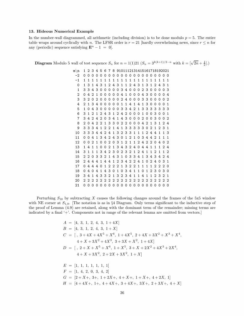
13. Hideous Numerical Example

In the number-wall diagrammed, all arithmetic (including division) is to be done modulo p = 5. The entiretable wraps around cyclically with n. The LFSR order is r = 21 [hardly overwhelming news, since r ≤ n forany (periodic) sequence satisfying En − 1 = 0].

Diagram Modulo 5 wall of test sequence Sn for n = 1(1)21 (Sn = 3k(k+1)/2−n with k = [

√2n+ 12 ].)

m\n 1 2 3 4 5 6 7 8 9101112131415161718192021

-2 0 0 0 0 0 0 0 0 0 0 0 0 0 0 0 0 0 0 0 0 0

-1 1 1 1 1 1 1 1 1 1 1 1 1 1 1 1 1 1 1 1 1 1

0 1 3 1 4 3 1 2 4 3 1 1 2 4 3 1 3 1 2 4 3 1

1 3 3 4 3 0 0 0 0 0 3 4 0 0 0 2 3 0 0 0 0 3

2 0 4 2 1 0 0 0 0 0 4 1 0 0 0 4 3 0 0 0 0 4

3 3 2 0 2 0 0 0 0 0 2 4 0 0 0 3 3 0 0 0 0 2

4 2 1 3 4 0 0 0 0 0 1 1 4 1 4 1 3 0 0 0 0 1

5 1 0 4 3 0 0 0 0 0 3 3 4 2 1 3 3 3 3 3 3 3

6 3 1 2 1 2 4 3 1 2 4 2 0 0 0 1 0 0 3 0 0 1

7 3 4 2 4 2 0 3 4 1 4 3 0 0 0 2 0 0 3 0 0 2

8 2 0 4 2 2 1 3 3 0 2 2 0 0 0 4 2 1 3 1 2 4

9 3 3 3 4 1 2 2 1 4 1 3 3 3 3 3 0 2 1 2 3 1

10 3 3 3 4 4 2 4 1 3 2 3 3 1 1 1 2 4 4 1 1 3

11 0 0 4 1 3 4 2 4 3 0 1 2 1 0 3 4 4 2 1 1 1

12 0 0 2 1 0 0 2 0 3 1 2 1 1 2 4 2 2 0 4 0 2

13 1 4 1 1 0 0 2 1 3 4 3 2 4 0 4 4 1 1 1 2 4

14 3 1 1 1 3 4 2 3 0 2 3 2 1 2 4 1 1 2 1 1 2

15 2 2 0 3 3 2 1 4 3 1 0 3 3 4 1 3 4 3 4 2 4

16 2 4 4 4 1 4 4 1 2 3 4 2 2 4 1 0 2 4 0 3 1

17 0 4 4 4 0 1 2 2 2 1 3 2 2 1 1 1 1 2 2 2 0

18 0 4 0 4 1 4 3 0 1 0 3 4 1 1 0 1 2 3 0 3 0

19 3 4 1 4 3 3 2 1 3 2 3 4 1 1 4 1 1 2 3 2 1

20 2 2 2 2 2 2 2 2 2 2 2 2 2 2 2 2 2 2 2 2 2

21 0 0 0 0 0 0 0 0 0 0 0 0 0 0 0 0 0 0 0 0 0

Perturbing S10 by subtracting X causes the following changes around the frames of the 5x5 windowwith NE corner at S1,9. [The notation is as in §4 Diagram. Only terms significant to the inductive step ofthe proof of Lemma (4.9) are retained, along with the dominant term of the remainder; missing terms areindicated by a final ‘+’. Components not in range of the relevant lemma are omitted from vectors.]

A = [4, 3, 1, 2, 4, 3, 1 + 4X ]

B = [4, 3, 1, 2, 4, 3, 1 +X ]

C = [ , 3 + 4X + 4X5 +X6, 1 + 4X5, 2 + 4X + 3X2 +X3 +X4,

4 +X + 3X2 + 4X3, 3 + 3X +X2, 1 + 4X ]

D = [ , 2 +X +X5 +X6, 1 +X5, 3 +X + 2X2 + 4X3 + 2X4,

4 +X + 3X2, 2 + 2X + 3X2, 1 +X ]

E = [1, 1, 1, 1, 1, 1, 1]

F = [1, 4, 2, 0, 3, 4, 2]

G = [2 +X+, 3+, 1 + 2X+, 4 +X+, 1 +X+, 4 + 2X, 1]

H = [4 + 4X+, 1+, 4 + 4X+, 3 + 4X+, 3X+, 2 + 3X+, 4 +X ]

36

M = N = [ , 4X5, 3X4, X3, 2X2, 4X, 3]

P = Q = 2 U = V = 2/X

R = 2 + 4X + 3X2 +X3 + 2X4 + 2X5 + 2X6+

T = 3 +X + 2X2 + 4X3 + 3X4 + 3X5 +X6+

To illustrate the perturbed frame results of §4, we show the dominant term of the error in (4.7),(4.8),(4.9):

err(C) = [ , , 4X5+, X5+, 2X3+, 2X3+, 2X+]

err(D) = [ , , 3X5+, 2X5+, 4X3+, 2X3+, X+]

err(PT/QR) = 4X6+

err(E + F +G+H) = [0+, 3X+, 4X+, 3X+, 3X+, X+, 4X+]

Now suppose that we knew the Frame Theorems for 4× 4 only, and had computed the original table asfar as the bottom of the 5× 5 window. To compute the South frames of this square, we might proceed thus:First perturb the table as above, then find N by (4.2), D by (4.3), H by (3.6) since N is now nonzero, andfinally let X → 0. The inductive versions of these theorems for g − 1 in the form required in the perturbedtable for 1 ≤ k ≤ k + 1 are:

Nk = (−)(g−1)(k−1)MkBk−1/Ak − 1Dk = (Nk/U)(QEk−1/Ak−1 − (−1)k(PFk−1/Bk−1 − V Ck/Mk))Hk = (Dk

2 −Dk−1Dk+1)/Nk

Notice how we need to compute D to O(X6) in order to be able to compute H2 to O(X) — i.e. at all —because N2 = 4X

5.But all this is idle speculation, since we do know the Frame Theorems for all g, and can simply compute

the original frames directly by (5.1).

37

References

Ait62 Aitken, A. Determinants and Matrices, Oliver & Boyd (1962).Bak75 Baker, G. A. Jr. Essentials of Pade Approximants, Academic Press (1975).Bla96 Blackburn, S. R. & Etzion, T. & Paterson, K. G. Permutation Polynomials, deBruijn Sequences, and

Linear Complexity, J. Comb. Theory ser. A 76 (1996) 55–82.Cha82 Chan, A. H. & Games, R. A. & Key, E. L. On the Complexities of deBruijn Sequences, J. Comb. Theory

ser. A 33 (1982) 55–82.Con96 Conway, J. H. & Guy, R. K. The Book of Numbers, Springer (1996).Dav88 Davenport, J. H. & Siret, Y. & Tournier, E. Computer Algebra, Academic Press (1988).Fay94 Faybusovich, Leonid Rational functions, Toda flows, and LR-like algorithms, Linear Algebra Appl.

203–204 (1994) 359–383.Fro85 Froberg, C-E. Numerical Mathematics, Benjamin Cummings (1985).Gil78 Gilewicz, Jacek Approximants de Pade, Springer Lecture Notes in Mathematics 667 (1978).Gra72 Gragg, W. B. The Pade Table and its Relation to Certain Algorithms of Numerical Analysis, SIAM

Review 14 (1972) 1–62.Gra96 Granville, A. The Arithmetic Properties of Binomial Coefficients, in Proceedings of the Organic Math-

ematics Workshop (1996).Hen74 Henrici, P. Applied and Computational Complex Analysis, Wiley (1974).Her75 Herstein, N. Topics in Algebra, ed. 2, Wiley (1975).Ioh82 Iohvidov, I. S. Hankel and Toeplitz Matrices and Forms, (trans. Thijsse, G. P. A.) Birkhauser (1982).Knu81 Knuth, D. The Art of Computer Programming, 1,2 ed 2, Addison-Wesley (1981).Lan93 Lang, S. Algebra, Addison-Wesley (1993).Lid86 Lidl, R. & Niederreiter, H. Introduction to Finite Fields and their Applications, Cambridge (1986).Lun00 Lunnon, W. F. Pagodas and Sackcloth: Ternary Sequences of Considerable Linear Complexity, (to

appear).Maz86 Mazoyer, J. An Overview of the FSSP, in C. Choffrut (ed) Automata Networks, Springer (1986) 82–94.Maz87 Mazoyer, J. A Six-State Minimal-Time Solution to the FSSP, Theoretical Computer Science 50 (1987)

183–238.Min67 Minsky, M. Computation: Finite and Infinite Machines, Prentice-Hall (1967).Nie89 Niederreiter, H. Keystream Sequences with a Good Linear Complexity Profile for Every Starting Point,

in Eurocrypt ’89 Abstracts Houthalen, Holland (1989).Niv69 Niven, Ivan Formal Power Series, Amer. Math. Monthly 76 (1969) 871–889.Pap94 Papageorgiou, V. & Grammaticos, B. & Ramani, A. Integrable difference equations and numerical

analysis algorithms, pp. 269-280 in Levi, Decio (ed.) et al. Symmetries and integrability of differenceequations: Papers from the workshop, May 22–29, 1994, Esterel, Canada; Amer. Math. Soc. Proc. Lect.Notes 9, 1996.

Poo96 van der Poorten, Alf Notes on Fermat’s Last Theorem, Wiley (1996)Ree85 Reeds, J. A. & Sloane, N. J. A. Shift-Register Synthesis (Modulo m), SIAM J. Computing 14 (1985)

505–513.Ris74 Rissanen, J. Solution of Linear Equations with Hankel and Toeplitz Matrices, Numer. Math. 22 (1974)

361–366.Rob86 Robbins, D. P. & Rumsey Jr., H. Determinants and Alternating Sign Matrices, Adv. in Math. 62 (1986)

169–184.Sen92 Sendra, J. R. & Llovat, J. Rank of a Hankel Matrix over Z[x1 . . . xr], Appl. Algebra in Eng. Comm. and

Computing 3 (1992) 245–256.Slo95 Sloane, N. J. A. & Plouffe, S. The Encyclopedia of Integer Sequences, Academic Press (1995).Ste92 Stephens, N. M. The Zero-square Algorithm for Computing Linear Complexity Profiles, in Mitchell,

Chris (ed.) Cryptography and Coding II, Clarendon press Oxford (1992) 259–272.Wyn60 Wynn, P. The Rational Approximation of Functions which are Formally Defined by a Power-Series

Expansion, Math. Comp.14 (1960) 147–186.Wyn66 Wynn, P. Upon Systems of Recursions which Obtain among the Quotients of the Pade Table, Numer.

Math. 8 (1966) 264–269.

38