
2 Discrete Dynamical Systems: Maps
86
19 2 Discrete Dynamical Systems: Maps 2.1 Introduction Many physical systems displaying chaotic behavior are accurately described by mathematical models derived from well-understood physical principles. For ex- ample, the fundamental equations of fluid dynamics, namely the Navier–Stokes equations, are obtained from elementary mechanical and thermodynamical con- siderations. The simplest laser models are built from Maxwell’s laws of electro- magnetism and from the quantum mechanics of a two-level atom. Except for stationary regimes, it is in general not possible to find closed-form solutions to systems of nonlinear partial or ordinary differential equations (PDEs and ODEs). However, numerical integration of these equations often reproduces surprisingly well the irregular behaviors observed experimentally. Thus, these mod- els must have some mathematical properties that are linked to the occurrence of chaotic behavior. To understand what these properties are, it is clearly desirable to study chaotic dynamical systems whose mathematical structure is as simple as possible. Because of the difficulties associated with the analytical study of differential systems, a large amount of work has been devoted to dynamical systems whose state is known only at a discrete set of times. These are usually defined by a rela- tion X nC1 D f ( X n ) (2.1) where f W M ! M is a map of a state space into itself and X n denotes the state at the discrete time n. The sequence f X n g obtained by iterating (2.1) starting from an initial condition X 0 is called the orbit of X 0 , with n 2 N or n 2 Z, depending on whether or not map f is invertible. If X 0 is chosen at random, one observes generally that its orbit displays two distinct phases: a transient that is limited in time and specific to the orbit, and an asymptotic regime that persists for arbitrarily long times and is qualitatively the same for different typical orbits. Rather than study individual orbits, we are interested in classifying all the asymptotic behaviors that can be observed in a dynamical system. The Topology of Chaos, Second Edition. Robert Gilmore, Marc Lefranc © 2011 WILEY-VCH Verlag GmbH & Co. KGaA. Published 2011 by WILEY-VCH Verlag GmbH & Co. KGaA
Transcript of 2 Discrete Dynamical Systems: Maps

19
2
Discrete Dynamical Systems: Maps
2.1
Introduction
Many physical systems displaying chaotic behavior are accurately described bymathematical models derived from well-understood physical principles. For ex-ample, the fundamental equations of fluid dynamics, namely the Navier–Stokesequations, are obtained from elementary mechanical and thermodynamical con-siderations. The simplest laser models are built from Maxwell’s laws of electro-magnetism and from the quantum mechanics of a two-level atom.
Except for stationary regimes, it is in general not possible to find closed-formsolutions to systems of nonlinear partial or ordinary differential equations (PDEsand ODEs). However, numerical integration of these equations often reproducessurprisingly well the irregular behaviors observed experimentally. Thus, these mod-els must have some mathematical properties that are linked to the occurrence ofchaotic behavior. To understand what these properties are, it is clearly desirableto study chaotic dynamical systems whose mathematical structure is as simple aspossible.
Because of the difficulties associated with the analytical study of differentialsystems, a large amount of work has been devoted to dynamical systems whosestate is known only at a discrete set of times. These are usually defined by a rela-tion
XnC1 D f (Xn) (2.1)
where f W M ! M is a map of a state space into itself and Xn denotes the stateat the discrete time n. The sequence fXng obtained by iterating (2.1) starting froman initial condition X0 is called the orbit of X0, with n 2 N or n 2 Z, dependingon whether or not map f is invertible. If X0 is chosen at random, one observesgenerally that its orbit displays two distinct phases: a transient that is limited intime and specific to the orbit, and an asymptotic regime that persists for arbitrarilylong times and is qualitatively the same for different typical orbits. Rather thanstudy individual orbits, we are interested in classifying all the asymptotic behaviorsthat can be observed in a dynamical system.
The Topology of Chaos, Second Edition. Robert Gilmore, Marc Lefranc© 2011 WILEY-VCH Verlag GmbH & Co. KGaA. Published 2011 by WILEY-VCH Verlag GmbH & Co. KGaA

20 2 Discrete Dynamical Systems: Maps
To understand the generic properties of chaotic behavior, there is no loss of gen-erality in restricting ourselves to discrete-time systems; it is often easy to extractsuch a system from a continuous-time system. A common example is provided bythe technique of Poincaré sections, where the study is narrowed to the dynamicsof the map relating the successive intersections of a trajectory with a given surfaceof phase space, which is usually called the first return map. Another example is thetime-one map X(t C 1) D φ1(X(t)) of a differential system, which relates two stateslocated one time unit apart along the same trajectory.
It might seem natural to restrict our study to discrete-time dynamical systemssharing some key properties with differential systems. For example, the solution ofa system of ODEs depends continuously on initial conditions, so that continuousmaps are naturally singled out. Invertibility is also a crucial property. Given aninitial condition, the state of an ODE system can in principle be determined atany time in the future but also in the past; thus, we must be able to go backwardin time. Maps satisfying these two requirements (i.e., continuous maps with acontinuous inverse) are called homeomorphisms. Another important class of mapsis made of diffeomorphisms: These are homeomorphisms that are differentiable aswell as their inverse.
The most important aspects of chaotic behavior should appear in systems oflowest dimension. Thus, we would like in a first step to reduce as much as possi-ble the dimension of state space. However, this quickly conflicts with the require-ment of invertibility. On the one hand, it can be shown that maps based on a one-dimensional homeomorphism can only display stationary or periodic regimes, andhence cannot be chaotic. On the other hand, if we sacrifice invertibility temporari-ly, thereby introducing singularities, one-dimensional chaotic systems can easily befound, as illustrated by the celebrated logistic map. Indeed, this simple system willbe seen to display many of the essential features of deterministic chaos.
It is, in fact, no coincidence that chaotic behavior appears in its simplest formin a noninvertible system. As emphasized in this book, singularities and nonin-vertibility are intimately linked to the mixing processes (stretching and squeezing)associated with chaos.
Because of the latter, a dissipative invertible chaotic map becomes formally non-invertible when infinitely iterated (i.e., when the phase space has been infinitelysqueezed). Thus the dynamics is, in fact, organized by an underlying singular mapof lower dimension, as can be shown easily in model systems such as the horse-shoe map. A classical example of this is the Hénon map, a diffeomorphism of theplane into itself that is known to have the logistic map as a backbone.
2.2
Logistic Map
A noninvertible one-dimensional map has at least one point where its derivativevanishes. The simplest such maps are quadratic polynomials, which can alwaysbe brought to the form f (x ) D a � x2 under a suitable change of variables. The

2.2 Logistic Map 21
-2
-1.5
-1
-0.5
0
0.5
1
1.5
2
-2 -1.5 -1 -0.5 0 0.5 1 1.5 2
x n+
1
xn
-2
-1.5
-1
-0.5
0
0.5
1
1.5
2
-2 -1.5 -1 -0.5 0 0.5 1 1.5 2
x n+
1
xn(a) (b)
Figure 2.1 (a) Graph of the logistic map for a D 2; (b) graphical representation of the iteration
of (2.2).
logistic map1)
xnC1 D a � x2n (2.2)
which depends on a single parameter a, is thus the simplest one-dimensional mapdisplaying a singularity. As can be seen from its graph (Figure 2.1a), the most im-portant consequence of the singularity located at the critical point x D 0 is thateach value in the range of the map f has exactly two preimages, which will proveto be a key ingredient to generate chaos. Maps with a single critical point are calledunimodal. It will be seen later that all unimodal maps display very similar dynami-cal behavior.
As is often the case in dynamical systems theory, the action of the logistic mapcan be represented not only algebraically, as in (2.2), but also geometrically. Givena point xn , the graph of the logistic map provides y D f (xn). To use y as thestarting point of the next iteration, we must find the corresponding location in thex space, which is done simply by drawing the line from the point [xn , f (xn)] to thediagonal y D x . This simple construction is then repeated ad libitum, as illustratedin Figure 2.1b.
The various behaviors displayed by the logistic map are easily explored, as thismap depends on a single parameter a. As illustrated in Figure 2.2, one finds quicklythat two main types of dynamical regimes can be observed: stationary or periodicregimes on the one hand, and “chaotic” regimes on the other hand. In the firstcase, iterations eventually visit only a finite set of different values that are foreverrepeated in a fixed order. In the latter case, the state of the system never repeatsitself exactly and seemingly evolves in a disordered way, as in Figure 2.1b. Bothtypes of behaviors have been observed in the experiment discussed in Chapter 1.
What makes the study of the logistic map so important is not only that the organi-zation in parameter space of these periodic and chaotic regimes can be completely
1) A popular variant is xnC1 D λxn (1 � xn ), with parameter λ.

22 2 Discrete Dynamical Systems: Maps
-2
-1
0
1
2
0 20 40 60 80 100
x n
n
-2
-1
0
1
2
x n
-2
-1
0
1
2
x n
(c)
(b)
(a)
Figure 2.2 Different dynamical behaviors observed in the logistic map system are represented
by plotting successive iterates: (a) stationary regime, a D 0.5; (b) periodic regime of period 5,
a D 1.476; (c) chaotic regime, a D 2.0.
understood with simple tools, but that, despite its simplicity, it displays the mostimportant features of low-dimensional chaotic behavior. By studying how period-ic and chaotic behavior are interlaced, we will learn much about the mechanismsresponsible for the appearance of chaotic behavior. Moreover, the logistic map isnot only a paradigmatic system: One-dimensional maps will later prove also to bea fundamental tool for understanding the topological structure of flows.
2.3
Bifurcation Diagrams
A first step in classifying the dynamical regimes of the logistic map is to obtaina global representation of the various regimes that are encountered as control pa-rameter a is varied. This can be done with the help of bifurcation diagrams, whichare tools commonly used in nonlinear dynamics. Bifurcation diagrams displaysome characteristic property of the asymptotic solution of a dynamical system asa function of a control parameter, allowing one to see at a glance where qualita-tive changes in the asymptotic solution occur. Such changes are termed bifurca-tions.
In the case of the logistic map that has a single dynamical variable, the bifur-cation diagram is readily obtained by plotting a sample set of values of the se-quence (xn) as a function of parameter a, as shown in Figure 2.3.
For a < a0 D �1/4, iterations of the logistic map escape to infinity from allinitial conditions. For a > aR D 2 almost all initial conditions escape to infinity.

2.3 Bifurcation Diagrams 23
-2
-1.5
-1
-0.5
0
0.5
1
1.5
2
0 0.5 1 1.5 2
x n
a
(i) (ii)(iii) (iv) (v)
Figure 2.3 Bifurcation diagram of the logis-
tic map. For a number of parameter values
between a D �0.25 and a D 2.0, 50 suc-
cessive iterates of the logistic map are plotted
after transients have died out. From left to
right, the vertical lines mark the creations of
(i) a period-2 orbit; (ii) a period-4 orbit; (iii) a
period-8 orbit, and (iv) the accumulation point
of the period-doubling cascade; (v) the start-
ing point of a period-3 window.
The bifurcation diagram is thus limited to the range a0 < a < aR , where boundedsolutions can be observed.
Between a0 D �1/4 and a1 D 3/4, the limit set consists of a single value. Thiscorresponds to a stationary regime, but one that should be considered in this con-text as a period-1 periodic orbit. At a D a1, a bifurcation occurs, giving birth to aperiod-2 periodic orbit: Iterations oscillate between two values. As detailed in Sec-tion 2.4.2, this is an example of a period-doubling bifurcation. At a D a2 D 5/4,there is another period-doubling bifurcation where the period-2 orbit gives birth toa period-4 orbit.
The period-doubling bifurcations occurring at a D a1 and a D a2 are the firsttwo members of an infinite series, known as the period-doubling cascade, in whichan orbit of period 2n is created for every integer n. The bifurcation at a D a3 leadingto a period-8 orbit is easily seen in the bifurcation diagram of Figure 2.3, the one ata D a4 is hardly visible, and the following ones are completely indiscernible to thenaked eye. This is because the parameter values an at which the period-2n orbit iscreated converge geometrically to the accumulation point a1 D 1.401 155 189 . . .with a convergence ratio substantially larger than 1:
limn!1
an � an�1
anC1 � anD δ � 4.669 201 609 1 . . . (2.3)
The constant δ appearing in (2.3) was discovered by Feigenbaum [22, 37] andis named after him. This distinction is justified by a remarkable property: Period-doubling cascades observed in an extremely large class of systems (experimental or

24 2 Discrete Dynamical Systems: Maps
-2
-1.5
-1
-0.5
0
0.5
1
1.5
2
1.4 1.5 1.6 1.7 1.8 1.9 2
x n
a
6 8 7 5 7 8 3 6 8 7 858 7 8687 48 78687858786878
Figure 2.4 Enlarged view of the chaotic zone of the bifurcation diagram of Figure 2.3. Inside
periodic windows of period up to 8, vertical lines indicate the parameter values where the corre-
sponding orbits are most stable, with the period indicated above the line.
theoretical, defined by maps or differential equations . . . ) have a convergence rategiven by δ.
At the accumulation point a1, the period of the solution has become infinite.Right of this point, the system can be found in chaotic regimes, as can be guessedfrom the abundance of dark regions in this part of the bifurcation diagram, whichindicate that the system visits many different states. The period-doubling cascade isone of the best-known routes to chaos and can be observed in many low-dimensionalsystems [10]. It has many universal properties that are in no way restricted to thecase of the logistic map.
However, the structure of the bifurcation diagram is more complex than a simpledivision between periodic and chaotic regions on both sides of the accumulationpoint of the period-doubling cascade. For example, a relatively large periodic win-dow, which corresponds to the domain of stability of a period-3 orbit, is clearly seento begin at a D 7/4, well inside the chaotic zone. In fact, periodic windows andchaotic regions are arbitrarily finely interlaced, as illustrated by Figure 2.4. As willbe shown later, there are infinitely many periodic windows between any two peri-odic windows. To interpret Figure 2.4, it should be noted that periodic windows arevisible to the naked eye only for very low periods. For higher periods, (i) the peri-odic window is too narrow compared to the scale of the plot and (ii) the numberof samples is sufficiently large that the window cannot be distinguished from thechaotic regimes.
Ideally, we would like to determine for each periodic solution the range of pa-rameter values over which it is stable. In Section 2.4 we will perform this analysisfor the simple cases of the period-1 and period-2 orbits, so that we get a better un-derstanding of the two types of bifurcation that are encountered in a logistic map.This is motivated by the fact that these are the two bifurcations that are genericallyobserved in low-dimensional dynamical systems (omitting the Hopf bifurcation,which we discuss later).

2.4 Elementary Bifurcations in the Logistic Map 25
However, we will not attempt to go much further in this direction. First, thecomplexity of Figures 2.3 and 2.4 shows that this task is out of reach. Moreover,we are only interested in properties of the logistic map that are shared by manyother dynamical systems. In this respect, computing exact stability ranges for alarge number of regimes would be pointless.
This does not imply that a deep understanding of the structure of the bifurcationdiagram of Figure 2.3 cannot be achieved. Quite to the contrary, we will see laterthat simple topological methods allow us to answer precisely the following ques-tions: How can we classify the different periodic regimes? Does the succession ofdifferent dynamical regimes encountered as parameter a is increased follow a logi-cal scheme? In particular, a powerful approach to chaotic behavior, symbolic dynam-ics, which we present in Section 2.7, will prove to be perfectly suited for unfoldingthe complexity of chaos.
2.4
Elementary Bifurcations in the Logistic Map
2.4.1
Saddle–Node Bifurcation
The simplest regime that can be observed in the logistic map is the period-1 orbit.It is stably observed on the left of the bifurcation diagram of Figure 2.3 for a0 <
a < a1. It corresponds to a fixed point of the logistic map (i.e., it is mapped ontoitself) and is thus a solution of the equation x D f (x ). For the logistic map, findingthe fixed points merely amounts to solving the quadratic equation
x D a � x2 (2.4)
which has two solutions:
x�(a) D �1 � p1 C 4a
2xC(a) D �1 C p
1 C 4a2
(2.5)
The fixed points of a one-dimensional map can also be located geometrical-ly, since they correspond to the intersections of its graph with the diagonal (Fig-ure 2.1).
Although a single period-1 regime is observed in the bifurcation diagram, thereare actually two period-1 orbits. Later we will see why. Expressions (2.5) are real-valued only for a > a0 D �1/4. Below this value, all orbits escape to infinity.Thus, the point at infinity, which we denote x1 in what follows, can formally beconsidered as another fixed point of the system, albeit unphysical.
The important qualitative change that occurs at a D a0 is our first exampleof a ubiquitous phenomenon of low-dimensional nonlinear dynamics, a tangent,or saddle–node, bifurcation: The two fixed points (2.5) become simultaneously realand are degenerate: x�(a0) D xC(a0) D �1/2. The two designations point to twodifferent (but related) properties of this bifurcation.

26 2 Discrete Dynamical Systems: Maps
-4
-3
-2
-1
0
1
2
-4 -3 -2 -1 0 1 2
x n+
1
xn
1 23
4
Figure 2.5 The basin of attraction of the xC
fixed point is located between the left fixed
point x� and its preimage, indicated by two
vertical lines. The orbits labeled 1 and 2 are
inside the basin and converge toward xC . The
orbits labeled 3 and 4 are outside the basin
and escape to infinity (i.e., converge to the
point at infinity x1).
The saddle–node qualifier is related to the fact that the two bifurcating fixedpoints have different stability properties. For a slightly above a0, it is found thatorbits located near xC converge to it, whereas those starting in the neighborhoodof x� leave it to either converge to xC or escape to infinity, depending on whetherthey are located right or left of x�. Thus, the fixed point xC (and obviously al-so x1) is said to be stable while x� is unstable. They are called the node and thesaddle, respectively.
Since trajectories in their respective neighborhoods converge to them, xC andx1 are attracting sets, or attractors. The sets of points whose orbits converge to anattractor of a system is called the basin of attraction of this point. From Figure 2.5we see that the unstable fixed point x� is on the boundary between the basins ofattraction of the two stable fixed points xC and x1. The other boundary point isthe preimage f �1(x�) of x� (Figure 2.5).
It is easily seen that the stability of a fixed point depends on the derivative of themap at the fixed point. Indeed, if we perturb a fixed point x� D f (x�) by a smallquantity δxn , the perturbation δxnC1 at the next iteration is given by
δxnC1 D f (x� C δxn) � x� D d f (x )dx
ˇˇ
x�
δxn C O�δx2
n
�(2.6)
If we start with an infinitesimally small δx0, the perturbation after n iterations isthus δxn � (μ�)n δx0, where μ�, the multiplier of the fixed point, is given by themap derivative at x D x�.
A fixed point is thus stable (resp. unstable) when the absolute value of its multi-plier is smaller (resp. greater) than unity. Here the multipliers μ˙ of the two fixed

2.4 Elementary Bifurcations in the Logistic Map 27
-2
-1.5
-1
-0.5
0
0.5
1
1.5
2
-2 -1.5 -1 -0.5 0 0.5 1 1.5 2
x n+
1
xn
Figure 2.6 Graph of the logistic map at the initial saddle–node bifurcation.
points of the logistic map are given by
μ� D d f (x )dx
ˇˇ
x�
D �2x� D 1 C p1 C 4a (2.7a)
μC D d f (x )dx
ˇˇ
xC
D �2xC D 1 � p1 C 4a (2.7b)
Equation 2.7a shows that x� is unconditionally unstable on its entire domain ofexistence, and hence is generically not observed as a stationary regime, whereasxC is stable for parameters a just above a0 D �1/4, as mentioned above. This iswhy only xC can be observed on the bifurcation diagram shown in Figure 2.3.
More precisely, xC is stable for a 2 [a0, a1], where a1 D 3/4 is such that μC D�1. This is consistent with the bifurcation diagram of Figure 2.3. Note that at a D0 2 [a0, a1], the multiplier μC D 0 and thus perturbations are damped out fasterthan exponentially: The fixed point is then said to be superstable.
At the saddle–node bifurcation, both fixed points are degenerate and their mul-tiplier is C1. This fundamental property is linked to the fact that at the bifurcationpoint, the graph of the logistic map is tangent to the diagonal (Figure 2.6), whichis why this bifurcation is also known as the tangent bifurcation. Tangency of twosmooth curves (here, the graph of f and the diagonal) is generic at a multiple inter-section point. This is an example of a structurally unstable situation: An arbitrarilysmall perturbation of f leads to two distinct intersections or no intersection at all(alternatively, to two real or to two complex roots).
It is instructive to formulate the intersection problem in algebraic terms. Thefixed points of the logistic equations are zeros of the equation G(x , a) D f (x I a) �x D 0. This equation defines implicit functions xC(a) and x�(a) of parameter a.In structurally stable situations, these functions can be extended to neighboringparameter values by use of the implicit function theorem.

28 2 Discrete Dynamical Systems: Maps
Assume that x�(a) satisfies G(x�(a), a) D 0 and that we shift parameter a by aninfinitesimal quantity δa. Provided that @G(x�(a), a)/@x ¤ 0, the correspondingvariation δx� in x� is given by
G(x , a) D G (x� C δx�, a C δa) D G(x , a) C @G@x
δx� C @G@a
δa D 0 (2.8)
which yields
δx� D �@G@a@G@x
δa (2.9)
showing that x�(a) is well defined on both sides of a if and only if @G/@x ¤ 0. Thecondition
@G (x�(a), a)@x
D 0 (2.10)
is thus the signature of a bifurcation point. In this case, the Taylor series (2.8) hasto be extended to higher orders of δx�. If @2G(x�(a), a)/@x2 ¤ 0, the variationδx� in the neighborhood of the bifurcation is given by
(δx�)2 D �2
@G@a
@2G@x2
δa (2.11)
From (2.11) we recover the fact that there is a twofold degeneracy at the bifur-cation point, two solutions on one side of the bifurcation and none on the otherside. The stability of the two bifurcating fixed points can also be analyzed: SinceG(x , a) D f (x I a) � x , their multipliers are given by μ� D 1 C @G(x�, a)/@x andare thus equal to 1 at the bifurcation.
Just above the bifurcation point, it is easy to show that the multipliers of the twofixed points xC and x� are given to leading order by μ˙ D 1� α
pjδaj, where thefactor α depends on the derivatives of G at the bifurcation point. It is thus genericthat one bifurcating fixed point is stable while the other one is unstable. In fact,this is a trivial consequence of the fact that the two nondegenerate zeros of G(x , a)must have derivatives @G/@x with opposite signs.
This is linked to a fundamental theorem, which we state below in the one-dimensional case but which can be generalized to arbitrary dimensions by replac-ing derivatives with Jacobian determinants. Define the degree of a map f as
deg f DX
f (xi )Dy
sgnd fdx
(xi ) (2.12)
where the sum extends over all the preimages of the arbitrary point y, and sgnz DC1 (resp. �1) if z > 0 (resp. z < 0). It can be shown that deg f does not depend

2.4 Elementary Bifurcations in the Logistic Map 29
on the choice of y provided that it is a regular value (the derivatives at its preimagesxi are not zero) and that it is invariant by homotopy. Let us apply this to G(x , a) fory D 0. Obviously, deg G D 0 when there are no fixed points, but also for any a sincethe effect of varying a is a homotopy. We thus see that fixed points must appear inpairs having opposite contributions to deg G . As discussed above, these oppositecontributions correspond to different stability properties at the bifurcation.
The discussion above shows that although we have introduced the tangent bi-furcation in the context of the logistic map, much of the analysis can be carriedto higher dimensions. In an n-dimensional state space, the fixed points are deter-mined by an n-dimensional vector function G . In a structurally stable situation,the Jacobian @G/@X has rank n. As one control parameter is varied, bifurcationswill be encountered at parameter values where @G/@X is of lower rank. If the Ja-cobian has rank n � 1, it has a single null eigenvector, which defines the directionalong which the bifurcation takes place. This explains why the essential features oftangent bifurcations can be understood from a one-dimensional analysis.
The theory of bifurcations is in fact a subset of a larger field of mathematics, thetheory of singularities [50, 51], which includes catastrophe theory [35, 49] as a specialimportant case. The tangent bifurcation is an example of the simplest type of sin-gularity: the fold singularity, which typically corresponds to twofold degeneracies.
In the next section we see an example of a threefold degeneracy, the cusp singu-larity, in the form of the period-doubling bifurcation.
2.4.2
Period-Doubling Bifurcation
As shown in Section 2.4.1, the fixed point xC is stable only for a 2 [a0, a1], withμC D 1 at a D a1 D �1/4 and μC D �1 at a D a1 D 3/4. For a > a1, both fixedpoints (2.5) are unstable, which precludes a period-1 regime. Just above the bifur-cation, what is observed instead is that successive iterates oscillate between twodistinct values (Figure 2.3), which comprise a period-2 orbit. This could have beenexpected from the fact that at a D a1, μC D �1 indicates that perturbations arereproduced every other period. The qualitative change that occurs at a D a1 (a fixedpoint becomes unstable and gives birth to an orbit of twice the period) is anotherimportant example of bifurcation: the period-doubling bifurcation, which is repre-sented schematically in Figure 2.7. Saddle–node and period-doubling bifurcationsare the only two types of local bifurcation that are observed for the logistic map.With the Hopf bifurcation, they are also the only bifurcations that occur genericallyin one-parameter paths in parameter space and, consequently, in low-dimensionalsystems.
Before we carry out the stability analysis for the period-2 orbit created at a D a1,an important remark has to be made. Expression (2.5) shows that the period-1 or-bit xC exists for every a > a0; hence it does not disappear at the period-doublingbifurcation but merely becomes unstable. It is thus present in all the dynamicalregimes observed after its loss of stability, including in the chaotic regimes of theright part of the bifurcation diagram of Figure 2.3. In fact, this holds for all the

30 2 Discrete Dynamical Systems: Maps
1
O2
O1O
Figure 2.7 Period-doubling bifurcation. Orbit O1 becomes
unstable in giving birth to orbit O2, whose period is twice that
of O1.
-0.5
0
0.5
1
1.5
0.5 0.6 0.7 0.8 0.9 1 1.1 1.2 1.3 1.4
x n
a
Figure 2.8 Orbits of period up to 16 of the period-doubling cascade. Stable (resp. unstable)
periodic orbits are drawn with solid (resp. dashed) lines.
periodic solutions of the logistic map. As an example, the logistic map at the tran-sition to chaos (a D a1) has an infinity of (unstable) periodic orbits of periods 2n
for any n, as Figure 2.8 shows.We thus expect periodic orbits to play an important role in the dynamics even
after they have become unstable. We will see later that this is indeed the case andthat much can be learned about a chaotic system from its set of periodic orbits,both stable and unstable.
Since the period-2 orbit can be viewed as a fixed point of the second iterate of thelogistic map, we can proceed as above to determine its range of stability. The twoperiodic points fx1, x2g are solutions of the quartic equation
x D f ( f (x )) D a � �a � x2�2
(2.13)
To solve for x1 and x2, we take advantage of the fact that the fixed points xC
and x� are obviously solutions of (2.13). Hence, we just have to solve the quadraticequation
p (x ) D f ( f (x )) � xf (x ) � x
D 1 � a � x C x2 D 0 (2.14)

2.4 Elementary Bifurcations in the Logistic Map 31
whose solutions are
x1 D 1 � p�3 C 4a2
x2 D 1 C p�3 C 4a2
(2.15)
We recover the fact that the period-2 orbit (x1, x2) appears at a D a1 D 3/4 andexists for every a > a1. By using the chain rule for derivatives, we obtain the mul-tiplier of the fixed point x1 of f 2 as
μ1,2 D d f 2(x )dx
ˇˇ
x1
D d f (x )dx
ˇˇ
x2
� d f (x )dx
ˇˇ
x1
D 4x1 x2 D 4(1 � a) (2.16)
Note that x1 and x2 viewed as fixed points of f 2 have the same multiplier, which isdefined to be the multiplier of the orbit (x1, x2). At the bifurcation point a D a1, wehave μ1,2 D 1, a signature of the two periodic points x1 and x2 being degenerate atthe period-doubling bifurcation.
However, the structure of the bifurcation is not completely similar to that of thetangent bifurcation discussed earlier. Indeed, the two periodic points x1 and x2 arealso degenerate with the fixed point xC. The period-doubling bifurcation of thefixed point xC is thus a situation where the second iterate f 2 has three degeneratefixed points. If we define G2(x , a) D f 2(x I a) � x , the signature of this threefolddegeneracy is G2 D @G2/@x D @2G2/@x2 D 0, which corresponds to a higher-order singularity than the fold singularity encountered in our discussion of thetangent bifurcation. This is, in fact, our first example of the cusp singularity. Notethat xC has a multiplier of �1 as a fixed point of f at the bifurcation and henceexists on both sides of the bifurcation; it merely becomes unstable at a D a1. Onthe contrary, x1 and x2 have multiplier 1 for the lowest iterate of f, of which theyare fixed points, and thus exist only on one side of the bifurcation.
We also may want to verify that deg f 2 D 0 on both sides of the bifurcation.Let us denote d(x�) as the contribution of the fixed point x� to deg f 2. We donot consider x�, which is not invoved in the bifurcation. Before the bifurcation,we have d(xC) D �1 (d f 2/dx (xC) < 1). After the bifurcation, d(xC) D 1 butd(x1) D d(x2) D �1, so that the sum is conserved.
The period-2 orbit is stable only on a finite parameter range. The other end ofthe stability domain is at a D a2 D 5/4, where μ1,2 D �1. At this parameter value,a new period-doubling bifurcation takes place, where the period-2 orbit loses itsstability and gives birth to a period-4 orbit. As shown in Figures 2.3 and 2.8, perioddoubling occurs repeatedly until an orbit of infinite period is created.
Although one might in principle repeat the analysis above for the successivebifurcations of the period-doubling cascade, the algebra involved quickly becomesintractable. Anyhow, the sequence of parameters an at which a solution of period 2n
emerges converges so quickly to the accumulation point a1 that this would be oflittle use, except perhaps to determine the exact value of a1, after which the firstchaotic regimes are encountered.
A fascinating property of the period-doubling cascade is that we do not need toanalyze directly the orbit of period 21 to determine very accurately a1. Indeed,
32 2 Discrete Dynamical Systems: Maps
it can be remarked that the orbit of period 21 is formally its own period-doubledorbit. This indicates some kind of scale invariance. Accordingly, it was recognizedby Feigenbaum that the transition to chaos in the period-doubling cascade can beanalyzed by means of renormalization group techniques [22, 37].
In this section we have analyzed how the periodic solutions of the logistic mapare created. After discussing changes of coordinate systems in the next section,we shall take a closer look at the chaotic regimes appearing in the bifurcation dia-gram of Figure 2.3. We will then be in a position to introduce more sophisticatedtechniques to analyze the logistic map, namely symbolic dynamics, and to gain acomplete understanding of the bifurcation diagram of a large class of maps of theinterval.
2.5
Map Conjugacy
2.5.1
Changes of Coordinates
The behavior of a physical system does not depend on how we describe it. Equa-tions defining an abstract dynamical system are meaningful only with respect to agiven parameterization of its states (i.e., in a given coordinate system). If we changethe parameterization, the dynamical equations should be modified accordingly sothat the same physical states are connected by the evolution laws.
Assume that we have a system whose physical states are parameterized by coor-dinates x 2 X , with an evolution law given by f W X ! X (i.e., xnC1 D f (xn)).If we switch to a new coordinate system specified by y D h(x ), with y 2 Y , thedynamical equations become ynC1 D g(yn), where the map g W Y ! Y satisfies
h( f (x )) D g(h(x )) (2.17)
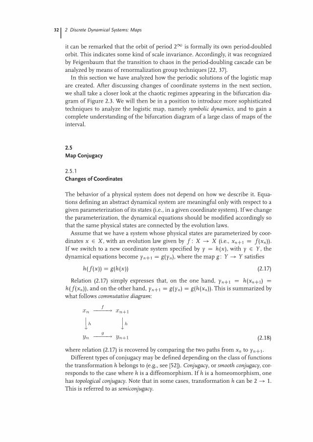
Relation (2.17) simply expresses that, on the one hand, ynC1 D h(xnC1) Dh( f (xn)), and on the other hand, ynC1 D g(yn) D g(h(xn)). This is summarized bywhat follows commutative diagram:
(2.18)
where relation (2.17) is recovered by comparing the two paths from xn to ynC1.Different types of conjugacy may be defined depending on the class of functions
the transformation h belongs to (e.g., see [52]). Conjugacy, or smooth conjugacy, cor-responds to the case where h is a diffeomorphism. If h is a homeomorphism, onehas topological conjugacy. Note that in some cases, transformation h can be 2 ! 1.This is referred to as semiconjugacy.

2.5 Map Conjugacy 33
2.5.2
Invariants of Conjugacy
Often, the problem is not to compute the evolution equations in a new coordinatesystem, but to determine whether two maps f and g correspond to the same physi-cal system (i.e., whether or not they are conjugate). A common strategy to addressthis type of problem is to search for quantities that are invariant under the classof transformations considered. If two objects have different invariants, they can-not be transformed into each other. The knot invariants discussed later provide animportant example of this. The ideal case is when there exists a complete set ofinvariants; equality of the invariants then implies identity of the objects. In thissection we present briefly two important invariants of conjugacy.
Spectrum of periodic orbits. An important observation is that there is a one-to-onecorrespondence between periodic orbits of two conjugate maps. Assume that x� isa period-p orbit of f W f p (x�) D x�. If f D h�1 ı g ı h, we have
f p D �h�1 ı g ı h
�p D h�1 ı g p ı h (2.19)
Thus, y� D h(x�) satisfies
y� D h ( f p (x�)) D g p (h(x�)) D g p (y�) (2.20)
This shows that y� is itself a period-p orbit of g. If h is a one-to-one transformation,it follows immediately that f and g have the same number of period-p orbits.
Of course, this should have been expected: The existence of a periodic solutiondoes not depend on the coordinate system. Yet this provides a useful criterion totest whether two maps are conjugate.
Multipliers of periodic orbits. Similarly, the stability and the asymptotic evolutionof a system are coordinate independent. In algebraic terms, this translates intothe invariance of the multipliers of a periodic orbit when transformation h is adiffeomorphism.
To show this, let us compute the tangent map D g p of g p D h ı f p ı h�1 at apoint y0, using the chain rule for derivatives:
D g p (y0) D D h��
f p ı h�1� (y0)� � D f p �h�1(y0)
� � D h�1(y0) (2.21)
To simplify notations, we set x0 D h�1(y0) and rewrite (2.21) as
D g p (y0) D D h ( f p (x0)) � D f p (x0) � D h�1(y0) (2.22)
Relation (2.22) yields no special relation between D f p (x0) and D g p (y0) unless x0
is a period-p orbit and satisfies f p (x0) D x0. In this case, indeed, we note that sinceD h( f p (x0)) D D h(x0), and because
D h�h�1(y0)
� � D h�1(y0) D 1 (2.23)

34 2 Discrete Dynamical Systems: Maps
we have
D g p (y0) D P � D f p (x0) � P�1 (2.24)
where P D D h(x0). Equation 2.24 indicates that the matrices D f p (x0) andD g p (y0) are similar: They can be viewed as two representations of the same linearoperator in two bases, with matrix P (obviously nonsingular since h is a diffeo-morphism) specifying the change of basis. Two matrices that are similar have,accordingly, the same eigenvalue spectrum.
This shows that the multipliers of a periodic orbit do not depend on the coordi-nate system chosen to parameterize the states of a system, and hence that they areinvariants of (smooth) conjugacy. Note, however, that they need not be preservedunder a topological conjugacy.
2.6
Fully Developed Chaos in the Logistic Map
The first chaotic regime that we study in the logistic map is the one observed at theright end of the bifurcation diagram, namely at a D 2. At this point, the logisticmap is surjective on the interval I D [�2, 2]: Every point y 2 I is the image of twodifferent points, x1, x2 2 I . I is then an invariant set since f (I ) D I .
It turns out that the dynamical behavior of a surjective logistic map can be ana-lyzed in a particularly simple way by using a suitable change of coordinates, namelyx D 2 sin(πx 0/4). This is a one-to-one transformation between I and itself, whichis a diffeomorphism everywhere except at the endpoints x D ˙2, where the inversefunction x 0(x ) is not differentiable. With the help of a few trigonometric identities,
-2
-1.5
-1
-0.5
0
0.5
1
1.5
2
-2 -1.5 -1 -0.5 0 0.5 1 1.5 2
x n+
1
xn
Figure 2.9 Graph of tent map (2.25).

2.6 Fully Developed Chaos in the Logistic Map 35
the action of the logistic map in the x 0 space can be written as
x 0nC1 D g(x 0
n) D 2 � 2ˇx 0
n
ˇ(2.25)
a piecewise linear map known as the tent map.Figure 2.9 shows that the graph of a tent map is extremely similar to that of a
logistic map (Figure 2.1). In both cases, interval I is decomposed into two subin-tervals: I D I0 [ I1, such that each restriction f k W Ik ! f (Ik ) of f is a homeomor-phism, with f (I0) D f (I1) D I . Moreover, f0 (resp. f1) is orientation-preserving(resp. orientation-reversing).
In fact, these topological properties suffice to determine the dynamics complete-ly and are characteristic features of what is often called a topological horseshoe. Inthe remainder of Section 2.6, we review a few fundamental properties of chaoticbehavior that can be shown to be direct consequences of these properties.
2.6.1
Iterates of the Tent Map
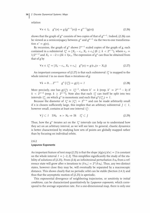
The advantage of the tent map over the logistic map is that calculations are sim-plified dramatically. In particular, higher-order iterates of the tent map, which areinvolved in the study of the asymptotic dynamics, are themselves piecewise-linearmaps and are easy to compute. For illustration, the graphs of the second iterate g2
and of the fourth iterate g4 are shown in Figure 2.10. Their structure is seen to bedirectly related to that of the tent map.
Much of the structure of the gn iterates can be understood from the fact that gmaps linearly each of the two subintervals I0 and I1 to the whole interval I. Thus,the graph of the restriction of g2 to each of the two components Ik reproduces thegraph of g on I. This explains the two-“hump” structure of g2. Similarly, the trivial
-2
-1.5
-1
-0.5
0
0.5
1
1.5
2
-2 -1.5 -1 -0.5 0 0.5 1 1.5 2
x n+
1
xn
Figure 2.10 Graphs of the second (heavy line) and fourth (light line) iterates of the tent map
(2.25).
36 2 Discrete Dynamical Systems: Maps
relation
8x 2 Ik gn(x ) D g�gn�1(x )
� D gn�1(g(x )) (2.26)
shows that the graph of gn consists of two copies of that of gn�1. Indeed, (2.26) canbe viewed as a semiconjugacy between gn and gn�1 via the two-to-one transforma-tion x 0 D g(x ).
By recursion, the graph of gn shows 2n�1 scaled copies of the graph of g, eachcontained in a subinterval I n
k D [Xk � �n , Xk C �n ] (0 � k < 2n�1), where �n D1/2n�2 and Xk D �2C (2k C1)�n . The expression of gn can thus be obtained fromthat of g by
8x 2 I nk D [Xk � �n , Xk C �n ] gn(x ) D g (�n(x � Xk )) (2.27)
An important consequence of (2.27) is that each subinterval I nk is mapped to the
whole interval I in no more than n iterations of g:
8k D 0 . . . 2n�1 gn �I nk
� D g(I ) D I (2.28)
More precisely, one has g(I nk ) D I n�1
k 0 , where k0 D k (resp. k0 D 2n�1 � k) ifk < 2n�2 (resp. k � 2n�2). Note also that each I n
k can itself be split into twointervals I n
k ,i on which gn is monotonic and such that gn(I nk ,i) D I .
Because the diameter of I nk is jI n
k j D 23�n and can be made arbitrarily smallif n is chosen sufficiently large, this implies that an arbitrary subinterval J I ,however small, contains at least one interval I n
k :
8 J I 9N0 n > N0 ) 9k I nk J (2.29)
Thus, how the gn iterates act on the I nk intervals can help us to understand how
they act on an arbitrary interval, as we will see later. In general, chaotic dynamicsis better characterized by studying how sets of points are globally mapped ratherthan by focusing on individual orbits.
2.6.2
Lyapunov Exponents
An important feature of tent map (2.25) is that the slope jdg(x )/dx j D 2 is constanton the whole interval I D [�2, 2]. This simplifies significantly the study of the sta-bility of solutions of (2.25). From (2.6) an infinitesimal perturbation δx0 from a ref-erence state will grow after n iterations to jδxnj D 2n jδx0j. Thus, any two distinctstates, however close they may be, will eventually be separated by a macroscopicdistance. This shows clearly that no periodic orbit can be stable (Section 2.4.1) andthus that the asymptotic motion of (2.25) is aperiodic.
This exponential divergence of neighboring trajectories, or sensitivity to initialconditions, can be characterized quantitatively by Lyapunov exponents, which corre-spond to the average separation rate. For a one-dimensional map, there is only one

2.6 Fully Developed Chaos in the Logistic Map 37
Lyapunov exponent, defined by
λ D limn!1
1n
n�1XiD0
logjδxnC1jjδxnj D lim
n!1
1n
n�1XiD0
logˇˇ d f
dx
�f i(x0)
�ˇˇ (2.30)
which is a geometric average of the stretching rates experienced at each iteration. Itcan be shown that Lyapunov exponents are independent of the initial condition x0,except perhaps for a set of measure zero [53].
Since the distance between infinitesimally close states grows exponentially asδxn � enλ δx0, sensitivity to initial conditions is associated with a strictly positiveLyapunov exponent. It is easy to see that the Lyapunov exponent of surjective tentmap (2.25) is λ D ln 2.
2.6.3
Sensitivity to Initial Conditions and Mixing
Sensitivity to initial conditions can also be expressed in a way that is more topolog-ical, without using distances. The key property we use here is that any subintervalJ I is eventually mapped to the whole I:
8 J I 9N0 n > N0 ) gn( J ) D I (2.31)
This follows directly from the fact that J contains one of the basis intervals I nk and
that these expand to I under the action of g; see (2.28) and (2.29).We say that a map is expansive if it satisfies property (2.31). In plain words, the
iterates of points in any subinterval can take every possible value in I after a suffi-cient number of iterations. Assume that J represents the uncertainty in the locationof an initial condition x0: We merely know that x0 2 J , but not its precise position.Then (2.31) shows that chaotic dynamics is, though deterministic, asymptoticallyunpredictable: After a certain amount of time, the system can be anywhere in thestate space. Note that the time after which all the information about the initial con-dition has been lost depends only logarithmically on the diameter j J j of J. Roughly,(2.28) indicates that N0 ' � ln j J j/ ln 2 � � ln j J j/λ.
In what follows, we use property (2.31) as a topological definition of chaos inone-dimensional noninvertible maps. To illustrate it, we recall the definitions ofvarious properties that have been associated with chaotic behavior [12] and whichcan be shown to follow from (2.31).
A map f W I ! I :
Has sensitivity to initial conditions if 9δ > 0 such that for all x 2 I and anyinterval J 3 x , there is a y 2 J and an n > 0 such that j f n(x ) � f n(y )j > δ.
Is topologically transitive if for each pair of open sets A, B I there exists n suchthat f n(A) \ B ¤ ;.
Is mixing if for each pair of open sets A, B I there exists N0 > 0 such thatn > N0 ) f n(A) \ B ¤ ;. A mixing map is obviously topologically transitive.
38 2 Discrete Dynamical Systems: Maps
Sensitivity to initial conditions trivially follows from (2.31) since any neighborhoodof x 2 I is eventually mapped to I. The mixing property, and hence transitivity, isalso a consequence of expansiveness because the N0 in the definition can be chosenso that f N0 (A) D I intersects any B I . It can be shown that a topologicallytransitive map has at least a dense orbit (i.e., an orbit that passes arbitrarily close toany point of the invariant set).
Note that (2.31) precludes the existence of an invariant subinterval J I otherthan I itself: We would have simultaneously f ( J ) D J and f N0 ( J ) D I for someN0. Thus, invariant sets contained in I necessarily consist of isolated points; theseare the periodic orbits discussed in the next section.
2.6.4
Chaos and Density of (Unstable) Periodic Orbits
It has been proposed by Devaney [12] to say that a map f is chaotic if it:
Displays sensitivity to initial conditions Is topologically transitive Has a set of periodic orbits that is dense in the invariant set.
The first two properties were established in Section 2.6.3. It remains to be provedthat (2.31) implies the third. When studying the bifurcation diagram of the logisticmap (Section 2.4.2), we have noted that chaotic regimes contain many (unstable)periodic orbits. We are now in a position to make this observation more precise. Webegin by showing that the tent map x 0 D g(x ) has infinitely many periodic orbits.
2.6.4.1 Number of Periodic Orbits of the Tent Map
A periodic orbit of g of period p is a fixed point of the pth iterate g p . Thus, it satisfiesg p (x ) D x and is associated with an intersection of the graph of g p with the diag-onal. Since g itself has exactly two such intersections (corresponding to period-1orbits), (2.27) shows that g p has
N f (p ) D 2p (2.32)
fixed points (see Figure 2.10 for an illustration).Some of these intersections might actually be orbits of lower period. For example,
the four fixed points of g2 consist of two period-1 orbits and of two points consti-tuting a period-2 orbit. As another example, note in Figure 2.10 that fixed points ofg2 are also fixed points of g4. The number of periodic orbits of lowest period p isthus
N(p ) D N f (p ) �Pq qN(q)
p(2.33)
where the q are the divisors of p. Note that this is a recursive definition of N(p ). Asan example, N(6) D [N f (6)�3N(3)�2N(2)�N(1)]/6 D (26 �3�2�2�1�2)/6 D 9,

2.6 Fully Developed Chaos in the Logistic Map 39
with the computation of N(3), N(2), and N(1) being left to the reader. As detailed inSection 2.7.5.3, one of these nine orbits appears in a period doubling and the eightothers are created by pairs in saddle–node bifurcations. Because N f (p ) increasesexponentially with p, N(p ) is well approximated for large p by N(p ) ' N f (p )/p .
We thus have the important property that there are an infinite number of pe-riodic points and that the number N(p ) of periodic orbits of period p increasesexponentially with the period. The corresponding growth rate,
hP D limp!1
1p
ln N(p ) D limp!1
1p
lnN f (p )
pD ln 2 (2.34)
provides an accurate estimate of a central measure of chaos, the topological en-tropy hT . In many cases it can be proven rigorously that hP D hT . Topologicalentropy itself can be defined in several different but equivalent ways.
2.6.4.2 Expansiveness Implies Infinitely Many Periodic Orbits
We now prove that if a continuous map f W I ! I is expansive, its unstable periodicorbits are dense in I: Any point x 2 I has periodic points arbitrarily close to it.Equivalently, any subinterval J I contains periodic points.
We first note that if J f ( J ) (this is a particular case of a topological covering),then J contains a fixed point of f as a direct consequence of the intermediate valuetheorem.2) Similarly, J contains at least one periodic point of period p if J f p ( J ).
Now, if (2.31) is satisfied, every interval J I is eventually mapped to I: f n( J ) DI (and thus f n( J ) J ) for n > N0( J ). Using the remark above, we deduce thatJ contains periodic points of period p for any p > N0( J ), but also possibly forsmaller p. Therefore, any interval contains an infinity of periodic points with arbitrarilyhigh periods. A graphical illustration is provided by Figure 2.10: Each intersectionof a graph with the diagonal corresponds to a periodic point.
Thus, the expansiveness property (2.31) implies that unstable periodic points aredense. We showed earlier that it also implies topological transitivity and sensitivityto initial conditions. Therefore, any map satisfying (2.31) is chaotic according tothe definition given at the beginning of this section.
It is quite fascinating that sensitivity to initial conditions, which makes the dy-namics unpredictable, and unstable periodic orbits, which correspond to perfectlyordered motion, are so deeply linked: In a chaotic regime, order and disorder areintimately entangled.
Unstable periodic orbits will prove to be a powerful tool to analyze chaos. Theyform a skeleton around which the dynamics is organized. Although they can becharacterized in a finite time, they provide invaluable information on the asymp-totic dynamics because of the density property: The dynamics in the neighborhoodof an unstable periodic orbit is governed largely by that orbit.
2) Denote by xa , xb 2 J the points such that f ( J ) D [ f (xa ), f (xb )]. If J � f ( J ), one has f (xa ) � xa
and xb � f (xb ). Thus, the function F(x ) D f (x ) � x has opposite signs in xa and xb . If f iscontinuous, F must take all the values between F(xa ) and F(xb ). Thus, there exists x� 2 J suchthat F(x�) D f (x�) � x� D 0: x� is a fixed point of f.
40 2 Discrete Dynamical Systems: Maps
2.6.5
Symbolic Coding of Trajectories: First Approach
We showed above that because of sensitivity to initial conditions, the dynamics ofthe surjective tent map is asymptotically unpredictable (Section 2.6.3). However,we would like to have a better understanding of how irregular, or random, typicalorbits can be. We also learned that there is a dense set of unstable periodic orbitsembedded in the invariant set I and that this set has a well-defined structure. Whatabout the other orbits, which are aperiodic?
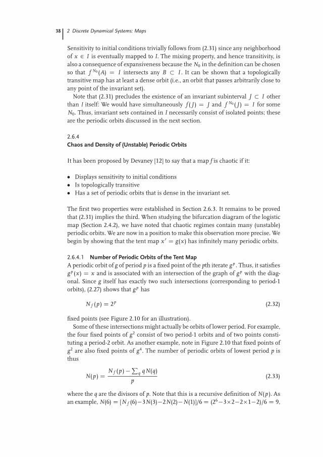
In this section we introduce a powerful approach to chaotic dynamics that an-swers these questions: symbolic dynamics. To do so as simply as possible, let usconsider a dynamical system extremely similar to the surjective tent map, definedby the map
xnC1 D 2xn (mod 1) (2.35)
It only differs from the tent map in that the two branches of its graph are bothorientation-preserving (Figure 2.11). As with the tent map, the interval [0, 1] is de-composed in two subintervals Ik such that the restrictions f k W Ik ! f k (Ik ) arehomeomorphisms.
The key step is to recognize that because the slope of the graph is 2 everywhere,the action of (2.35) is trivial if the coordinates x 2 [0, 1] are represented in base 2.Let xn have the binary expansion xn D 0.d0 d1 . . . dk . . ., with dk 2 f0, 1g. It is easyto see that the next iterate will be
xnC1 D (d0.d1 d2 . . . dk . . .) (mod 1) D 0.d1d2 . . . dk . . . (2.36)
Thus, the base-2 expansion of xnC1 is obtained by dropping the leading digit in theexpansion of xn . This leading digit indicates whether x is greater than or equal to
0
0.2
0.4
0.6
0.8
1
0 0.2 0.4 0.6 0.8 1
x n+
1
xn
Figure 2.11 Graph of map (2.35).
2.6 Fully Developed Chaos in the Logistic Map 41
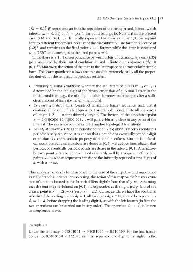
1/2 D 0.10 (s represents an infinite repetition of the string s) and, hence, whichinterval I0 D [0, 0.5) or I1 D [0.5, 1] the point belongs to. Note that in the presentcase, 0.10 and 0.01, which usually represent the same number 1/2, correspondhere to different trajectories because of the discontinuity. The former is located at(1/2)C and remains on the fixed point x D 1 forever, while the latter is associatedwith (1/2)� and converges to the fixed point x D 0.
Thus, there is a 1 W 1 correspondence between orbits of dynamical system (2.35)(parameterized by their initial condition x) and infinite digit sequences (dk ) 2f0, 1gN . Moreover, the action of the map in the latter space has a particularly simpleform. This correspondence allows one to establish extremely easily all the proper-ties derived for the tent map in previous sections.
Sensitivity to initial conditions: Whether the nth iterate of x falls in I0 or I1 isdetermined by the nth digit of the binary expansion of x. A small error in theinitial condition (e.g., the nth digit is false) becomes macroscopic after a suffi-cient amount of time (i.e., after n iterations).
Existence of a dense orbit: Construct an infinite binary sequence such that itcontains all possible finite sequences. For example, concatenate all sequencesof length 1, 2, . . . , n for arbitrarily large n. The iterates of the associated pointx D 0.0j1j00j01j10j11j000j001 . . . will pass arbitrarily close to any point of theinterval. The existence of a dense orbit implies topological transitivity.
Density of periodic orbits: Each periodic point of (2.35) obviously corresponds to aperiodic binary sequence. It is known that a periodic or eventually periodic digitexpansion is a characteristic property of rational numbers. Since it is a classi-cal result that rational numbers are dense in [0, 1], we deduce immediately thatperiodic or eventually periodic points are dense in the interval [0, 1]. Alternative-ly, each point x can be approximated arbitrarily well by a sequence of periodicpoints x�(n) whose sequences consist of the infinitely repeated n first digits ofx, with n ! 1.
This analysis can easily be transposed to the case of the surjective tent map. Sinceits right branch is orientation-reversing, the action of this map on the binary expan-sion of a point x located in this branch differs slightly from that of (2.36). Assumingthat the tent map is defined on [0, 1], its expression at the right (resp. left) of thecritical point is x 0 D 2(1� x ) (resp. x 0 D 2x ). Consequently, we have the additionalrule that if the leading digit is d0 D 1, all the digits di , i 2 N, should be replaced byQdi D 1 � di before dropping the leading digit d0 as with the left branch (in fact, thetwo operations can be carried out in any order). The operation di ! Qdi is knownas complement to one.
Example 2.1
Under the tent map, 0.010 010 11 ! 0.100 101 1 ! 0.110 100. For the first transi-tion, since 0.010 010 0 < 1/2, we shift the separator one digit to the right. In the

42 2 Discrete Dynamical Systems: Maps
second transition, since x D 0.100 101 1 > 1/2, we first complement x and obtainx 0 D (1 � x ) D 0.011 010 0, then multiply by 2: 2x 0 D 0.110 110 0.
Except for this minor difference in the coding of trajectories, the arguments usedabove to show the existence of chaos in the map x 0 D 2x (mod 1) can be followedwithout modification. The binary coding we have used is thus a powerful methodto prove that the tent map displays chaotic behavior.
The results of this section naturally highlight two important properties of chaoticdynamics:
A series of coarse-grained measurements of the state of a system can suffice toestimate it with arbitrary accuracy if carried out over a sufficiently long time. Bymerely noting which branch is visited (one-bit digitizer) at each iteration of themap (2.35), all the digits of an initial condition can be extracted.
Although a system such as (2.35) is perfectly deterministic, its asymptotic dy-namics is as random as coin flipping (all sequences of 0 and 1 can be observed).
However, the coding used in these two examples (n-ary expansion) is too naive to beextended to maps that do not have a constant slope equal to an integer. In the nextsection we discuss the general theory of symbolic dynamics for one-dimensionalmaps. This topological approach will prove to be an extremely powerful tool tocharacterize the dynamics of the logistic map, not only in the surjective case butfor any value of parameter a.
2.7
One-Dimensional Symbolic Dynamics
2.7.1
Partitions
Consider a continuous map f W I ! I that is singular. We would like to extendthe symbolic dynamical approach introduced in Section 2.6.5 in order to analyzeits dynamics. To this end, we have to construct a coding associating each orbit ofthe map with a symbol sequence.
We note that in the previous examples, each digit of the binary expansion of apoint x indicates whether x belongs to the left or right branch of the map. Accord-ingly, we decompose interval I in N disjoint intervals Iα, α D 0 . . . N �1 (numberedfrom left to right), such that
I D I0 [ I1 [ � � � IN�1
In each interval Iα , the restriction f jIα W Iα ! f (Iα), which we denote f α , is ahomeomorphism.

2.7 One-Dimensional Symbolic Dynamics 43
I0 I1 I2 I3 I4
x
f (x)
Figure 2.12 Decomposition of the domain of a map f into intervals Iα such that the restrictions
f W Iα ! f (Iα) to the intervals Iα are homeomorphisms.
For one-dimensional maps, such a partition can easily be constructed by choosingthe critical points of the map as endpoints of the intervals Iα , as Figure 2.12 il-lustrates. At each iteration, we record the symbol α 2 A D f0, . . . , N � 1g thatidentifies the interval to which the current point belongs. The alphabet A consistsof the N values that the symbol can assume.
We denote by s(x ) the corresponding coding function:
s(x ) D α () x 2 Iα (2.37)
Any orbit fx , f (x ), f 2(x ), . . . , f i (x ), . . .g of initial condition x can then be associat-ed with the infinite sequence of symbols indicating the intervals visited successive-ly by the orbit:
Σ(x ) D ˚s(x ), s( f (x )), s
�f 2(x )
�, . . . , s
�f i(x )
�, . . .
�(2.38)
The sequence Σ(x ) is called the itinerary of x. We will also use the compact notationΣ D s0 s1 s2 . . . s i . . ., with the s i being the successive symbols of the sequence (e.g.,Σ D 01101001 . . .). The set of all possible sequences in the alphabet A is denotedAN , and Σ(I ) AN represents the set of sequences actually associated with apoint of I:
Σ(I ) D fΣ(x )I x 2 I g (2.39)
The finite sequence made of the n leading digits of Σ(x ) will later be useful. Wedenote it Σn(x ). For example, if Σ(x ) D 10110 . . ., then Σ3(x ) D 101. Accordingly,the set of finite sequences of length n involved in the dynamics is Σn(I ).
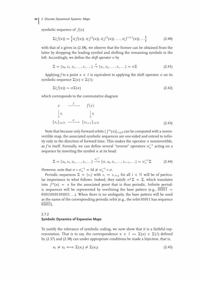
An important property of the symbolic representation (2.38) is that the expres-sion of the time-one map becomes particularly simple. Indeed, if we compare the
44 2 Discrete Dynamical Systems: Maps
symbolic sequence of f (x )
Σ( f (x )) Dn
s( f (x )), s( f 2(x )), s( f 3(x )), . . . , s( f iC1(x )), . . .o
(2.40)
with that of x given in (2.38), we observe that the former can be obtained from thelatter by dropping the leading symbol and shifting the remaining symbols to theleft. Accordingly, we define the shift operator σ by
Σ D fs0, s1, s2, . . . , s i , . . .g σ! fs1, s2, . . . , s i , . . .g D σΣ (2.41)
Applying f to a point x 2 I is equivalent to applying the shift operator σ on itssymbolic sequence Σ(x ) 2 Σ(I ):
Σ( f (x )) D σΣ(x ) (2.42)
which corresponds to the commutative diagram
(2.43)
Note that because only forward orbits f f n(x )gn�0 can be computed with a nonin-vertible map, the associated symbolic sequences are one-sided and extend to infin-ity only in the direction of forward time. This makes the operator σ noninvertible,as f is itself. Formally, we can define several “inverse” operators σ�1
α acting on asequence by inserting the symbol α at its head:
Σ D fs0, s1, s2, . . . , s i , . . .g σ�1α�! fα, s0, s1, . . . , s i�1, . . .g D σ�1
α Σ (2.44)
However, note that σ ı σ�1α D Id ¤ σ�1
α ı σ.Periodic sequences Σ D fs ig with s i D s iCp for all i 2 N will be of particu-
lar importance in what follows. Indeed, they satisfy σ p Σ D Σ, which translatesinto f p (x ) D x for the associated point that is thus periodic. Infinite period-ic sequences will be represented by overlining the base pattern (e.g., 01011 D010110101101011 . . .). When there is no ambiguity, the base pattern will be usedas the name of the corresponding periodic orbit (e.g., the orbit 01011 has sequence01011).
2.7.2
Symbolic Dynamics of Expansive Maps
To justify the relevance of symbolic coding, we now show that it is a faithful rep-resentation. That is to say, the correspondence x 2 I $ Σ(x ) 2 Σ(I ) definedby (2.37) and (2.38) can under appropriate conditions be made a bijection, that is,
x1 ¤ x2 () Σ(x1) ¤ Σ(x2) (2.45)

2.7 One-Dimensional Symbolic Dynamics 45
We might additionally require some form of continuity so that sequences that areclose according to some metric are associated with points that are close in space.
In plain words, the symbolic sequence associated to a given point is sufficient todistinguish it from any other point in interval I. The two dynamical systems (I, f )and (Σ(I ), σ) can then be considered as equivalent, with Σ(x ) playing the role ofa change of coordinate. Partitions of state space that satisfy (2.45) are said to begenerating.
In Section 2.6.5, we saw two particular examples of one-to-one correspondencebetween orbits and symbolic sequences. Here we show that such a bijection holds ifthe following two conditions are true: (i) The restriction of the map to each memberof the partition is a homeomorphism (Section 2.7.1) and (ii) the map satisfies theexpansiveness property (2.31). This will illustrate the intimate connection betweensymbolic dynamics and chaotic behavior.
In the tent map example, it is obvious how the successive digits of the binaryexpansion of a point x specify the position of x with increasing accuracy. As weshow below, this is also true for general symbolic sequences under appropriateconditions.
As a simple example, assume that a point x has a symbol sequence Σ(x ) D101 . . . From the leading symbol we extract the top-level information about the po-sition of x, namely that x 2 I1. Since the second symbol is 0, we deduce thatf (x ) 2 I0 (i.e., x 2 f �1(I0)). This second-level information combined with the
first-level information indicates that x 2 I1 \ f �1(I0) � I10. Using the first threesymbols, we obtain x 2 I101 D I1 \ f �1(I0) \ f �2(I1) D I1 \ f �1(I0 \ f �1(I1)).We note that longer symbol sequences localize the point with higher accuracy:I1 I10 I101.
More generally, define the interval IΛ D Is0 s1...sn�1 as the set of points whosesymbolic sequence begins by the finite sequence Λ D s0 s1 . . . sn�1, the remainingpart of the sequence being arbitrary:
IΛ D Is0 s1...sn�1 D fx I Σn(x ) D s0 s1 . . . sn�1gD ˚
x I s( f i(x )) D s i , i < n�
D ˚x I f i (x ) 2 Is i , i < n
�(2.46)
Such sets are usually termed cylinders, with an n-cylinder being defined by a se-quence of length n. We now show that cylinders can be expressed simply usinginverse branches of function f. We first define
8 J I f �1α ( J ) D Iα \ f �1( J ) (2.47)
This is a slight abuse of notation since we have only that f α ( f �1α ( J )) J without
the equality being always satisfied, but it makes the notation more compact. Withthis convention, the base intervals Iα can be written as
Iα D fx I s(x ) D αg D f �1α (I ) 8α 2 A (2.48)

46 2 Discrete Dynamical Systems: Maps
To generate the whole set of cylinders, this expression can be generalized to longersequences by noting that
IαΛ D f �1α (IΛ) (2.49)
which follows directly from definitions (2.46) and (2.47). Alternatively, (2.49) canbe seen merely to express that αΛ D σ�1
α Λ. By applying (2.49) recursively, oneobtains
IΛ D f �nΛ (I ) (2.50)
where f �nΛ is defined by
f �nΛ D f �n
s0 s1...sn�1D f �1
s0ı f �1
s1ı � � � ı f �1
sn�1(2.51)
Just as the restriction of f to any interval Iα is a homeomorphism f α W Iα ! f (Iα),the restriction of f n to any set IΛ with Λ of length n is a homeomorphism3)
f nΛ W IΛ ! f n(IΛ). The function f �n
Λ defined by (2.51) is the inverse of thishomeomorphism, which explains the notation. For a graphical illustration, see Fig-ure 2.10: Each interval of monotonic behavior of the graph of g2 (resp. g4) corre-sponds to a different interval IΛ , with Λ of length 2 (resp. 4).
Note that because I is connected and the f �1α are homeomorphisms, all the IΛ
are connected sets and, hence, are intervals in the one-dimensional context. Thisfollows directly from (2.49) and the fact that the image of a connected set by ahomeomorphism is a connected set. This property will be important in what fol-lows.
To illustrate relation (2.50), we apply it to the case Λ D 101 considered in theexample above:
I101 D ( f �11 ı f �1
0 ı f �11 )(I ) D ( f �1
1 ı f �10 )(I1)
D f �11 (I0 \ f �1(I1))
D I1 \ f �1(I0 \ f �1(I1))
and verify that it reproduces the expression obtained previously.The discussion above shows that the set of n cylinders Cn D fIΛI Λ 2 Σn(I )g is
a partition of I:
I D[
Λ2Σn (I )
IΛ IΛ \ IΛ0 D ; (2.52)
with Cn being a refinement of Cn�1 (i.e., each member of Cn is a subset of a mem-ber of Cn�1). As n ! 1, the partition Cn becomes finer and finer (again, seeFigure 2.10). What we want to show is that the partition is arbitrarily fine in thislimit, with the size of each interval of the partition converging to zero.
3) Note that f n is a homeomorphism only on set IΛ defined by symbolic strings Λ of length p � n(e.g., f 2 has a singularity in the middle of I0).

2.7 One-Dimensional Symbolic Dynamics 47
0 1
y
x x10
Figure 2.13 The dashed line indicates the border of a partition such that the preimages x0 and
x1 of the same point y are coded with the same symbol (0). As a consequence, the symbolic
sequences associated to x0 and x1 are identical.
Consider an arbitrary symbolic sequence Σ(x ), with Σn(x ) listing its n leadingsymbols. Since by definition IΣnC1(x ) IΣn (x ), the sequence (IΣn(x ))n2N is decreas-ing, hence it converges to a limit IΣ (x ). All the points in IΣ (x ) share the same infinitesymbolic sequence.
As the limit of a sequence of connected sets, IΣ (x ) is itself a connected set and,hence, an interval or an isolated point. Assume that IΣ (x ) is an interval. Then, be-cause of the expansiveness property (2.31), there is N0 such that f N0 (IΣ (x )) D I .This implies that for points x 2 IΣ (x ), the symbol sN0 D s( f N0 )(x ) can take anyvalue α 2 A, in direct contradiction of IΣ (x ) corresponding to a unique sequence.Thus the only possible solution is that the limit IΣ (x ) is an isolated point, show-ing that the correspondence between points and symbolic sequences is one to one.Therefore, the symbolic dynamical representation of the dynamics is faithful.
This demonstration assumes a partition of I constructed so that each interval ofmonotonicity corresponds to a different symbol (Figure 2.12). This guarantees thatall the preimages of a given point will be associated with different symbols sincethey belong to different intervals.
It is easy to see that partitions not respecting this rule cannot be generating. As-sume that two points x0 and x1 have the same image f (x0) D f (x1) D y andthat they are coded with the same symbol s(x0) D s(x1) D αk (Figure 2.13). Theyare then necessarily associated with the same symbolic sequence, consisting of thecommon symbol αk concatenated with the symbolic sequence of their commonimage: Σ(x0) D Σ(x1) D αk Σ(y ). In other words, associating x0 and x1 with differ-ent symbols is the only chance to distinguish them because they have exactly thesame future.
In one-dimensional maps, two preimages of a given point are always separatedby a critical point. Hence, the simplest generating partition is obtained by merelydividing the base interval I into intervals connecting two adjacent critical pointsand associating each with a different symbol.

48 2 Discrete Dynamical Systems: Maps
Remark 1: This is no longer true for higher-dimensional noninvertible maps,which introduces some ambiguity in the symbolic coding of trajectories.
Remark 2: Invertible chaotic maps do not have singularities, hence the construc-tion of generating partitions is more involved. The forthcoming examples ofthe horseshoe and of the Hénon map will help us to understand how the rulesestablished in the present section can be generalized.
2.7.3
Grammar of Chaos: First Approach
Symbolic dynamics provides a simple but faithful representation of a chaotic dy-namical system (Section 2.7.2). It has allowed us to understand the structure of thechaotic and periodic orbits of the surjective tent map, and hence of the surjectivelogistic map (Section 2.6.5). But there is more.
As a control parameter of a one-dimensional map varies, the structure of its in-variant set and of its orbits changes (perestroika). Symbolic dynamics is a powerfultool to analyze these modifications: As orbits are created or destroyed, symbolicsequences appear or disappear from the associated symbolic dynamics. Thus, aregime can be characterized by a description of its set of forbidden sequences. Werefer to such a description as the grammar of chaos. Changes in the structure of amap are characterized by changes in this grammar.
As we illustrate below with simple examples, which sequences are allowed andwhich are not can be determined entirely geometrically. In particular, the orbit ofthe critical point plays a crucial role. The complete theory, namely kneading theory,is detailed in Section 2.7.4.
2.7.3.1 Interval Arithmetics and Invariant Interval
We begin by determining the smallest invariant interval I (i.e., such that f (I ) D I ).This is where the asymptotic dynamics will take place. Let us first show how tocompute the image of an arbitrary interval J D [xl , xh ]. If J is located entirely tothe left or right of the critical point xc , one merely needs to take into account thatthe logistic map is orientation-preserving (resp. orientation-reversing) at the left(resp. right) of xc . Conversely, if xc 2 J , then J can be decomposed as [xl , xh ] D[xl , xc) [ [xc , xh ]. This gives
f ([xl , xh ]) D
8<ˆ:�
f (xl ), f (xh)�
if xl , xh � xc�f (xh), f (xl )
�if xc � xl , xh�
minf f (xl ), f (xh)g, f (xc)�
if xl � xc � xh
(2.53)
As was noted by Poincaré, the apparent complexity of chaotic dynamics is suchthat it makes little sense to follow individual orbits; what is relevant is how regionsof the state space are mapped between each other. One-dimensional maps are noexception, and in fact many properties of the logistic map can be extracted from

2.7 One-Dimensional Symbolic Dynamics 49
the interval arithmetics defined by (2.53). Here we use them to show in a simpleway that some symbolic sequences are forbidden.
Let us now determine I D [xmin, xmax] such that f (I ) D I . We are interested onlyin situations where this interval contains the critical point, so that the dynamics isnontrivial. Note that this implies that xc � f (xc) because we must have xc Df (y ) � f (xc) (hence the top of the parabola must be above the diagonal). We use
the third case of (2.53) to obtain the equation�minf f (xmin), f (xmax)g, f (xc)
� D [xmin, xmax] (2.54)
The upper bound is thus the image of the critical point: xmax D f (xc). The lowerbound xmin satisfies the equation
xmin D min f f (xmin), f (xmax)g D min˚
f (xmin ), f 2(xc)�
(2.55)
An obvious solution is xmin D f 2(xc), which is valid provided that f ( f 2(xc)) >
f 2(xc). This is always the case between the parameter value where the period-1orbit is superstable and the one where bounded solutions cease to exist. The otherpossible solution is the fixed point x� D f (x�). In the parameter region of inter-est, however, one has x� < f 2(xc), and thus the smallest invariant interval is givenby
I D �f 2(xc), f (xc)
�(2.56)
That it depends only on the orbit of the critical point xc is remarkable. However,this merely prefigures Section 2.7.4, where we shall see that this orbit determinesthe dynamics completely. Note that I ¤ ; as soon as f (xc ) > xc , which is the onlyinteresting parameter region from a dynamical point of view.
2.7.3.2 Existence of Forbidden Sequences
As shown previously, the set IΛ of points whose symbolic sequence begins by thefinite string Λ is given by IΛ D f �n
Λ (I ), where f �nΛ is defined by (2.51) and (2.47).
It is easy to see that if IΛ D ;, the finite symbol sequence Λ is forbidden.From the discussion above, the base intervals are
I0 D �f 2(xc), xc
�I1 D �
xc , f (xc)�
(2.57)
which are nonempty for f (xc) > xc . The existence of symbolic sequences of lengthtwo is determined by the intervals
I00 D I0 \ f �10 (I0) D �
f 2(xc), f �10 (xc)
�(2.58a)
I01 D I0 \ f �10 (I1) D �
f �10 (xc), xc
�(2.58b)
I10 D I1 \ f �11 (I0) D �
f �11 (xc), f (xc )
�(2.58c)
I11 D I1 \ f �11 (I1) D �
xc , f �11 (xc)
�(2.58d)

50 2 Discrete Dynamical Systems: Maps
-2
-1.5
-1
-0.5
0
0.5
1
1.5
2
-2 -1.5 -1 -0.5 0 0.5 1 1.5 2
x n+
1
xn
xcf0-1(xc) f1
-1(xc)
f 2(xc)
f(xc)
I00 I01 I11 I10
Figure 2.14 Intervals I00, I01, I11, and I10 defined in (2.58). In each interval, the itineraries have
the same leading two symbols.
which are computed by means of the interval arithmetics (2.53) but can also beobtained graphically (Figure 2.14). The last three do not provide useful information:They are nonempty whenever f (xc) > xc , i.e., as soon as I given by (2.56) is welldefined.
By contrast, (2.58a) yields a nontrivial condition for I00 to be nonempty, namelythat f 2(xc) < f �1
0 (xc). This interval has zero width when its two bounds are equal;thus the string “00” becomes allowed when the critical point belongs to a period-3orbit:
f 2(xc) D f �10 (xc) ) f 3(xc) D xc (2.59)
which is then superstable since the derivative of f is zero at the critical point. Forthe logistic map (2.2), this occurs precisely at a D a00 D 1.754 877 66 . . ., inside theunique period-3 window that can be seen in the bifurcation diagram of Figure 2.3.
Since I00 D ; for a < a00, we conclude that the symbolic string “00” neverappears in the symbolic dynamics of regimes located at the left of the period-3window. Thus the presence or absence of this string is sufficient to distinguishregimes located before and after this window.
In particular, this has consequences for the order of the appearance of periodicorbits. The first periodic orbit carrying the “00” string is the period-3 orbit 001.Therefore, all other periodic orbits whose names contain “00,” for example 001011,must appear after 001. This shows that the geometrical structure of the map has adeep influence on the order of appearance of periodic orbits, as detailed later in amore systematic way.
Reproducing the calculation above for longer symbolic strings, we would findthat new symbolic sequences always appeared when the critical point was part of aperiodic orbit (i.e., at the parameter inside the periodic window where the orbit issuperstable). This is not surprising if we note that the bounds of all the IΛ intervalscan be expressed in terms of the images and preimages of the critical point xc .
2.7 One-Dimensional Symbolic Dynamics 51
As a result, the condition of zero width of these intervals can always be rewrittenas an equation of the type f �n
Λ (xc) D xc , expressing that x belongs to a periodicorbit of period n and of symbolic sequence Λ. For example, (2.59) corresponds tof �3
100 (xc) D xc . However, we will not proceed in this direction. The observationthat the grammar of the symbolic dynamics is governed completely by the orbit ofthe critical point will lead us to a much more efficient framework for classifyingsymbolic sequences of orbits.
We conclude this section with the important remark that the symbolic dynam-ics of a chaotic dynamical system is in general intimately related to its geometricalstructure. In the case of unimodal maps, the structure of the forbidden sequencesdepends only on the position of the image of the critical point organizing the dy-namics. Thus, given an arbitrary symbolic sequence, it is in principle possible todetermine whether it has been generated by a one-dimensional map. More gen-erally, extracting the structure of a map from the grammar of the symbolic dy-namics it generates is a fascinating problem. It has been much less explored fortwo-dimensional invertible maps than for maps of the interval, and even less fornoninvertible maps of dimension 2 and higher.
2.7.4
Kneading Theory
Rather than solve algebraic equations such as (2.59) to determine forbidden se-quences, it would be preferable to work completely in the space of symbolic se-quences. Since the orbit of the critical point plays a crucial role in understandingwhich symbolic sequences are forbidden, it is natural to study more closely thedistinguished symbolic sequence associated with the critical point.
Since the first symbol of this sequence does not carry any information (the crit-ical point xc is the border between intervals I0 and I1), we accordingly define thekneading sequence K( f ) as the itinerary of the image of xc :
K( f ) D Σ ( f (xc)) D ˚s ( f (xc)) , s
�f 2(xc)
�, . . .
�(2.60)
Note that the first two symbols are constant inside the parameter region wheref 2(xc) < xc < f (xc ): f 2(xc) and f (xc) are the left and right ends of the invariant
interval I defined in (2.56) and are thus associated with the symbols 0 and 1, respec-tively. Since the value of the third symbol depends on whether f 3(xc) is located tothe left or right of the critical point, it changes when f 3(xc) D xc (i.e., when thestring “00” becomes allowed), and thus
a < a00 ) K( f ) D f1, 0, 1, . . .ga > a00 ) K( f ) D f1, 0, 0, . . .g (2.61)
This confirms the importance of the kneading sequence (2.60): The appearance ofthe symbolic string “00” in the symbolic dynamics of the logistic map coincideswith its appearance in the kneading sequence.
52 2 Discrete Dynamical Systems: Maps
To go beyond this observation, we need to be able to determine from K( f ) alonewhich sequences are allowed and which are not. The distinctive property of f (xc )is that it is the rightmost point of the invariant interval (2.56). To see that there isindeed a similar property for the kneading sequence, we first show that an orderon itineraries can be defined.
2.7.4.1 Ordering of Itineraries
In the example of the xnC1 D 2xn (mod 1) map (Section 2.6.5), the itinerary ofa point (i.e., its binary expansion) not only identifies it uniquely but also containsinformation about its position relative to the other points. In that case, the lexi-cographic order on symbolic sequences reflects exactly the order of the associatedpoints on the interval. More generally, we would like to define for an arbitrary mapan order relation � on itineraries so that
Σ(x ) � Σ�x 0� () x < x 0 (2.62)
Ordering two itineraries is easy when their leading symbols differ. If the baseintervals Iα are numbered sequentially from left to right as in Figure 2.12, theitinerary with the smallest leading symbol is associated with the leftmost point andshould be considered “smaller” than the other.
If the two itineraries have a common leading substring, one has to take intoaccount the fact that map f can be orientation-reversing on some Iα intervals. Forexample, the two-symbol cylinders Iαα0 given by (2.58) and shown in Figure 2.14appear left to right in the order I00, I01, I11, and I10.
Thus, 11 � 10 for the logistic map, which differs markedly from the lexicograph-ic order. This is because both strings have a leading 1, which is associated with theorientation-reversing branch f1. Indeed, assume that x11 2 I11, x10 2 I10. Fromthe second symbol we know that f (x10) < f (x11) because 0 < 1. However, since fis orientation-reversing in I1, this implies that x11 < x10, hence 11 � 10. With thispoint in mind, two arbitrary itineraries Σ , Σ0 can be ordered as follows.
Assume that the two sequences Σ D Λ sm . . . and Σ0 D Λ s0m . . . have a com-
mon leading symbolic string Λ of length m and first differ in symbols sm and s0m .
Thus the corresponding points x and x 0 are such that f m(x ) and f m(x 0) belongto different Iα intervals and, hence, can be ordered. As in the example above, itthen suffices to determine whether the restriction f m
Λ of f m to the interval IΛ isorientation-preserving or orientation-reversing (has a positive or a negative slope,respectively) to obtain the ordering of x and x 0, and thus that of Σ and Σ0. Definethe branch parity
�(α) D(C1 if f α W Iα ! I is orientation-preserving
�1 if f α W Iα ! I is orientation-reversing(2.63)
The parity of the finite sequence Λ D s0 s1 . . . sm�1 is then given by
�(Λ) D �(s0) � �(s1) � � � � � �(sm�1) (2.64)

2.7 One-Dimensional Symbolic Dynamics 53
0 1
0 1
01
111011010111 1011
Figure 2.15 Determination of the relative or-
der of symbolic sequences. White (resp. black)
nodes correspond to positive (resp. nega-
tive) parity. The topmost node corresponds
to the empty sequence, and sequences are
formed by following edges carrying the sym-
bols 0 or 1. When an edge “1” is followed,
the parity of the node changes. A white node
has an edge “0” on its left and an edge “1” on
its right (this is the lexicographic order). At a
black node, these two edges are in the oppo-
site order because of the negative parity. To
order a set of symbolic sequences, one follows
the edges corresponding to the successive
symbols of the sequence until no other se-
quence remains in the branch. The ordered
sequences can then be read from left to right.
If the map f mΛ D f sm�1 ı . . . f s1 ı f s0 (i.e., the restriction of f m to the interval IΛ)
is orientation-preserving (resp. orientation-reversing), then �(Λ) D C1 (resp. �1).In the case of unimodal maps, �(Λ) D C1 if there is an even number of “1” (or ofthe symbol associated with the orientation-reversing branch), and �1 otherwise.
We can now define the order
Σ D Λ s . . . � Σ0 D Λ s0 . . . ()
8<ˆ:
s < s0 and �(Λ) D C1
or
s > s0 and �(Λ) D �1
(2.65)
This order satisfies condition (2.62). Let us illustrate these rules with the exampleof period-4 orbit 0111 of the logistic map. The relative order of the four periodicorbits is
0111 � 1101 � 1110 � 1011 (2.66)
as detailed in Figure 2.15.Another common technique for ordering symbolic sequences is to use invariant
coordinates. Given a sequence Σ D s0 s1 s2 . . . sk . . . 2 f0, . . . , N � 1gN , we define itsinvariant coordinate θ (Σ) by
θ (Σ) D1X
iD0
ti
N iC1 ti D(
s i if �(s0 . . . s i�1) D C1
(N � 1) � s i if �(s0 . . . s i�1) D �1(2.67)
so that 0 � θ (Σ) � 1. By inspecting (2.65) and (2.67), one easily verifies that twosymbolic sequences can be ordered by comparing their invariant coordinates:
Σ � Σ0 () θ (Σ) < θ (Σ0) (2.68)

54 2 Discrete Dynamical Systems: Maps
As an example, the invariant coordinate of the periodic point 1011 of the logisticmap is
θ (1011) D�
121 C 1
22 C 023 C 1
24 C 025 C 0
26 C 127 C 0
28
�
��
1 C 128
C 1216
C � � ��
D 105128
� 256255
D 1417
(2.69)
where the digits in bold are those that have been inverted with respect to the orig-inal sequence. Because 1011 has negative parity, the binary digit sequence of θ (Σ)has period 8 instead of 4. The first factor in (2.69) corresponds to the basic pattern“11010010,” and the second term comes from the infinite repetition of this pat-tern. Note that the fraction obtained is the position of the corresponding periodicpoint of the tent map defined on [0, 1]. The reader may verify as an exercise that2 � j1 � θ (1011)j D θ (0111) and that 2 � θ (0111) D θ (1110).
2.7.4.2 Admissible Sequences
We showed earlier that each point x inside the invariant interval (2.56) satisfiesf 2(xc) < x < f (xc). Using (2.62), we can now translate this ordering relation
between points into a ordering relation between symbolic sequences:
8x 2 I σK( f ) � Σ(x ) � K( f ) (2.70)
since K( f ) D Σ( f (xc )), by definition. Moreover, the orbit of a point x 2 I isforever contained in I, by definition. A necessary condition for a sequence Σ to bethe itinerary Σ(x ) of a point x 2 I is thus that (2.70) holds for any Σ( f n(x )) andthus that
8n � 0 σn Σ � K( f ) (2.71)
One of the fundamental results of one-dimensional symbolic dynamics is thatthis is also a sufficient condition: Condition (2.71) completely determines whethera sequence occurs as the itinerary of a point [12, 52]. A sequence satisfying it is saidto be admissible (equivalently, one can test whether σK( f ) < σn Σ for all n).
Therefore, all the information about the symbolic dynamics of a map is containedin its kneading sequence K( f ). As a matter of fact, it can be shown that if two uni-modal maps have the same kneading sequence, and that if this sequence is dense(i.e., the orbit of xc is aperiodic), then the two maps are topologically conjugate.
Condition (2.71) is particularly simple to test when the symbolic sequence Σ isperiodic since the shifts σn Σ are finite in number. For example, let us assume thatK( f ) D 1001001 . . . and that we want to know whether the periodic sequences01101101 and 00101 are admissible. We first determine the rightmost periodicpoints (for which σn Σ is maximal) of the two orbits: These are 10110110 and 10010.We then compare them to the kneading sequence K( f ) and find that
10110110 � K( f ) D 1001001 . . . � 10010

2.7 One-Dimensional Symbolic Dynamics 55
Thus the period-8 sequence 10110110 is admissible, whereas the period-5 sequence10010 is not. This indicates that the periodic orbit associated with the latter se-quence does not exist in maps with the given K( f ). We also see that every mapthat has the second periodic orbit also has the first. Therefore, the order of ap-pearance of periodic orbits is fixed, and the structure of the bifurcation diagram ofFigure 2.3 is universal for unimodal maps. We investigate this universality in thenext section.
2.7.5
Bifurcation Diagram of the Logistic Map Revisited
We are now in a position to understand the structure of the bifurcation diagramshown in Figure 2.3 using the tools of symbolic dynamics introduced in the previ-ous sections. This bifurcation diagram displays two types of bifurcations: saddle–node and period-doubling bifurcations. Each saddle–node bifurcation creates a pairof periodic orbits of period p, one unstable (the saddle) and the other stable (thenode). The latter is the germ of a period-doubling cascade with orbits of periodsp � 2n .
As discussed in Section 2.7.4, the kneading sequence governs which symbol-ic sequences are admissible and which are forbidden, hence the order in whichnew sequences appear. Therefore, there must be a simple relation between thesymbolic names of the orbits involved in a saddle–node or in a period-doublingbifurcation. Moreover, the different saddle–node bifurcations and their associatedperiod-doubling cascades must be organized rigidly.
2.7.5.1 Saddle–Node Bifurcations
At a saddle–node bifurcation, the two newly born periodic orbits of period p areindistinguishable. Thus, they have formally the same symbolic name. This is notin contradiction with the one-to-one correspondence between orbits and itinerariesthat was shown to hold for chaotic regimes: At the bifurcation, the node is stableand there is no sensitivity to initial conditions.
When the two orbits are born, they have a multiplier of C1 (Section 2.4.1), whichimplies that f p is orientation-preserving in the neighborhood of the orbit. Con-sequently, the common symbolic itinerary of the two orbits must contain an evennumber of symbols “1” (in the general case, an even number of symbols with neg-ative parity).
A symbolic itinerary can change only if one of the periodic points crosses thecritical point, which is the border of the partition. This happens to the stable nodewhen it becomes superstable, changing its parity on its way to the period-doublingbifurcation where its multiplier crosses �1. Thus, its parity must be negative, andits final symbolic name (i.e., the one in the unstable regime) must differ from thatof the saddle by a single symbol.
One can proceed as follows to see which symbol differs. Each periodic point isassociated with a cyclic permutation of the symbolic name. For example, the orbit

56 2 Discrete Dynamical Systems: Maps
-2
-1.5
-1
-0.5
0
0.5
1
1.5
2
-2 -1.5 -1 -0.5 0 0.5 1 1.5 2
x n+
1
xn
Figure 2.16 The 01111 orbit becomes 01011 at a superstable point.
01111 has periodic points with sequences 01111, 11110, 11101, 11011, and 10111.These periodic points can be ordered using the kneading order (2.65), here
01111 � 11110 � 11011 � 11101 � 10111
The symbol that is flipped at the superstable parameter value is obviously asso-ciated with the point that is then degenerate with the critical point. The image ofthis point is thus the rightmost periodic point, corresponding to the highest se-quence in the kneading order (Figure 2.16). Consequently, a simple rule to obtainthe symbolic name of the saddle–node partner of an orbit of given name is to flipthe last symbol of the highest itinerary (i.e., of the itinerary of the rightmost point).Alternatively, one can flip the second to last symbol of the leftmost itinerary.
In the example above, the saddle–node partner of the 01111 orbit is thus 01101.Other examples of saddle–node pairs include 00
11, 00011, and 011010
11.
2.7.5.2 Period-Doubling Bifurcations
When applying the algorithm above on an arbitrary symbolic name, it can occurthat the result is not valid because it is the repetition of a shorter name. For exam-ple, 0111 leads to 0101 D (01)2. This indicates that the long name corresponds tothe period-doubled orbit (the daughter) of the orbit identified by the short name(the mother). The 0111 orbit is the daughter of the 01 orbit. The latter is itself thedaughter of the 1 orbit.
This can be understood with the same arguments as for the saddle–node bifur-cations. When the period-doubled orbit is born, its itinerary is a double copy of thatof the mother. Its parity is thus positive, which is consistent with the fact that theorbit is born with a multiplier of C1. The symbolic name of the mother at the bifur-cation is its final name. As the daughter orbit proceeds to its own period doubling(and thus to its unstable domain), the preimage of its rightmost point crosses thecritical point, changing the associated symbol.

2.7 One-Dimensional Symbolic Dynamics 57
Hence we have a simple way to determine whether an orbit belongs to a period-doubling cascade and what the names of its mother and all its ancestors are. Otherexamples of mother–daughter pairs are (001, 001011) and (00101, 0010100111). Weconclude with the period-doubling cascade originating from the period-1 orbit. Thesymbolic names of the successive period-doubled orbit can be constructed as
1D�! 11
F�! 01D�! 0101
F�! 0111D�! 01110111
F�! 01110101 � � � (2.72)
where D and F represent the action of doubling the word and flipping the secondto last symbol, respectively.
2.7.5.3 Universal Sequence
Consider two periodic itineraries Σ � Σ0. For some parameter a, the kneadingsequence K( f a) is such that Σ � K( f a) � Σ0, so that Σ satisfies the admissibilitycondition (2.71) but not Σ0. Thus, the periodic orbit associated to Σ must be createdbefore the one associated to Σ0.
This observation suffices to build a complete list of the successive bifurcationsoccurring in the bifurcation diagram of Figure 2.3. Using the rules derived in pre-vious sections, we can classify all the symbolic names according to which series ofbifurcations they belong to.
To this end, all periodic itineraries up to a given period p are sorted according tothe kneading order, with saddle–node pairs and orbits of the same period-doubling
Table 2.1 Sequence of bifurcations in the
logistic map up to period 8 (from top and
to bottom and left to right). The notation Pi
refers to the ith bifurcation of period P. We
also give inside brackets an alternative clas-
sification that distinguishes between saddle–
node and period-doubling bifurcations. In this
scheme, the ith saddle–node bifurcation of
period P is denoted siP , and si
P � 2k is the
orbit of period P � 2k belonging to the period-
doubling cascade originating from siP .
Name Bifurcation Name Bifurcation Name Bifurcation
01 11[s1] 001010
11 73[s37] 00010
11 64[s36]
01 21[s1 � 21] 001010011 85[s4
8] 000111011 811[s9
8]0111 41[s1 � 22] 0010
11 52[s25] 000110
11 77[s77]
01010111 81[s1 � 23] 001110011 86[s5
8] 000110011 812[s10
8 ]
0111011 61[s1
6] 00111011 74[s4
7] 000011 53[s3
5]0111110
11 82[s18] 0011110
11 87[s68] 0000100
11 813[s118 ]
01111011 71[s1
7] 0011011 63[s2
6] 00001011 78[s8
7]
011011 51[s1
5] 001101011 88[s7
8] 000011011 814[s12
8 ]011010
11 72[s27] 001100
11 75[s57] 00000
11 65[s46]
011011011 83[s2
8] 00011 42[s1
4] 000001011 815[s13
8 ]00
11 31[s3] 00010011 89[s14 � 21] 000000
11 79[s97]
001011 62[s3 � 21] 00010011 76[s6
7] 000000011 816[s14
8 ]
001011011 84[s3
8] 000101011 810[s8
8]

58 2 Discrete Dynamical Systems: Maps
cascade grouped together. We denote the ith bifurcation creating period-P orbits asPi , with the node being called Pi f (for flip) and the saddle Pi r (for regular). Thisis illustrated in Table 2.1, which lists the symbolic names of all periodic orbits ofperiod up to 8 of the logistic map. These names are sorted by order of appearance,and the bifurcation in which they appear is indicated.
This sequence of symbolic names, often referred to as the universal sequence, wasdiscovered by Metropolis, Stein, and Stein [5]. It is universal in that it depends onlyon the kneading order (2.65): The bifurcation diagram of any unimodal map willdisplay exactly the same bifurcations in exactly the same order.
Note, however, that this holds only for one-dimensional maps. If a two-dimen-sional map is sufficiently dissipative so that its return map can be well approxi-mated by a one-dimensional map, most of the bifurcation sequences will occur inthe order predicted by the universal sequence. However, there will be a few dis-crepancies, and the order of many bifurcations will be reversed as one decreasesdissipation [54].
2.7.5.4 Self-Similar Structure of the Bifurcation Diagram
In this section we mention briefly another surprising property of the bifurcationdiagram of the logistic map that is unveiled by symbolic dynamics. Look at theperiod-3 window beginning at a D 1.75 in Figure 2.4. There is a whole parameterrange where the attractor is contained in three disconnected pieces, before it ex-pands suddenly. These pieces are visited successively in a fixed order. We call thisparameter region the generalized period-3 window. Look more closely at, say, themiddle branch: This is a complete copy of the whole bifurcation diagram! In par-ticular, there is a period-9 window that is to the period-3 window what the period-3is itself to the whole diagram.
To understand this, we note that the base symbols 0 and 1 can be viewed asthe names of the period-1 orbits organizing the global dynamics. Similarly, let usdenote by X D 101 and Y D 100 the symbolic names of the two period-3 orbitsborn in the saddle–node bifurcation initiating the period-3 window. All periodicorbits appearing in the generalized period-3 window can be written as words in theletters X and Y.
Indeed, since the attractor is split into three pieces visited successively, the dy-namics can be simplified by considering the third iterate f 3. Each of the threepieces is a different attractor of f 3. The return map for each attractor is a unimodalmap, with two “period-1” orbits that are in fact periodic points of the two period-3orbits 100 and 101. Any pair of symbols X 0 and Y 0, such that the sequences X 0 andY 0 correspond to periodic points that are degenerate at the period-3 saddle–nodebifurcation, can thus be used to code orbits of this map. Because we chose X andY above to be higher in the kneading order than all their cyclic permutations, theysatisfy this condition as well as any pair σk X , σk Y .
Since the two words X D 101 and Y D 100 are such that (i) X � Y and (ii) theyhave parities �(X ) D C1 and �(Y ) D �1, it is easy to see that the ordering of two se-quences W1(X , Y ) and W2(X , Y ) will be exactly the same as for the corresponding

2.8 Shift Dynamical Systems, Markov Partitions, and Entropy 59
sequences W1(0, 1) and W2(0, 1). For example,
Y X Y Y X Y Y X � Y X X Y X () 10110110 � 10010
This explains why the bifurcation diagram in the generalized period-3 windowhas exactly the same structure as the whole diagram. Using the names of the stan-dard period-doubling cascade given in (2.72), we find that the orbits involved in theperiod-doubling cascade of this window are Y, X Y , X Y Y Y , X Y Y Y X Y X Y . Thefirst orbits to appear in the window are the X and Y orbits (naming them after theirsequences in the unstable regime); the last is the Y X 1 orbit.
In fact, the results of this section could have been foreseen: They are a conse-quence of the qualitative universality of bifurcations in unimodal maps. Inside theperiod-3 window, the third return map is a unimodal map and therefore displaysthe same series of bifurcations as the first return map.
2.8
Shift Dynamical Systems, Markov Partitions, and Entropy
In Section 2.7, we saw how a chaotic system can be analyzed with the tools ofsymbolic dynamics. In particular, each regime of the logistic map is characterizedby a different grammar (i.e., a set of forbidden symbolic sequences). Moreover,symbolic dynamics can be shown in some cases to provide a complete descriptionof a dynamical system; for example, it is known that chaotic unimodal maps areconjugate if they have the same kneading sequence.
It is thus natural to study systems whose evolution laws are defined directly in asymbolic space by rules specifying which sequences are admissible. Such systemsare usually referred to as symbolic dynamical systems, or as shift dynamical systemswhen they are based on the shift map [55]. Tools developed to characterize thesesystems can then be applied to any physical system for which a symbolic dynamicaldescription has been obtained. This is illustrated by computations of entropy, animportant measure of chaotic dynamics.
Here we limit ourselves to shifts of finite type, which are characterized by a finiteset of forbidden sequences. The interest of finite shifts is twofold. First, there aredynamical systems, those for which a Markov partition exists, that can be shown tobe equivalent to a finite shift. Second, systems whose grammar cannot be specifiedby a finite set of rules can always be approximated with increasing accuracy by asequence of finite shifts of increasing order.
2.8.1
Shifts of Finite Type and Topological Markov Chains
The natural phase space of a symbolic dynamical system is the set of infinite orbi-infinite sequences of symbols from an alphabet A. Here we assume that thealphabet is finite and choose A D f0, . . . , N�1g, where N is the number of symbols.

60 2 Discrete Dynamical Systems: Maps
The systems we consider here share the same time-one map: the shift operator σ,which shifts symbols one place to the left (Section 2.7.1).
In the case of the logistic map, the symbolic space consisted of one-sided sym-bolic sequences. We noted in Section 2.7.1 that this makes σ noninvertible, sincememory of the leading symbol is lost after each time step. If the shift operator hasto be invertible, its action must not discard information. Thus sequences must bebi-infinite (two-sided), for example,
Σ D . . . s�3 s�2 s�1.s0 s1 s2 (2.73)
with the dot separating the forward sequence ΣC D s0 s1 . . . from the backward se-quence Σ� D s�1 s�2 . . . These two sequences describe the future and the past ofthe point, respectively. The action of the shift operator on a sequence is then givenby
σ(. . . s�1.s0 s1 . . .) D . . . s�1s0.s1 . . .
The dot is merely moved to the right, which obviously preserves the informationcontained in the sequence. This is illustrated with the horseshoe map in Sec-tion 2.10.
The distinction between invertible and noninvertible dynamics is not made bymost methods developed for characterizing symbolic dynamical systems. As wesee below, they usually involve determining which finite blocks of symbols canappear in a typical sequence and which cannot. Thus, whether sequences are one-or two-sided is not relevant.
Full shifts are the simplest shift symbolic dynamical systems: Any sequence madeof letters of the alphabet is allowed. Thus the symbolic space is AN or AZ, de-pending on the invertibility of the dynamics. Two full shifts can differ only by thenumber of symbols of their alphabets. A full shift on r symbols is termed an r-shift.
In a general shift dynamical system, not all sequences are allowed: It is thencalled a subshift. We are interested only in subshifts whose set of allowed se-quences S is shift-invariant (i.e., σS D S). This implies that whether a finitesymbol string can be found in a sequence Σ 2 S depends not on its position in thesequence but only on the content of the string. Finite symbol strings are also oftenreferred to as blocks, with an n-block containing n symbols, or as words.
One could therefore provide a complete description of a dynamical system (S , σ)by specifying its language (i.e., the list of all finite strings of symbols that can beextracted from infinite sequences). It is usually much more convenient to specifyits set F of irreducible forbidden words (IFWs). An IFW never appears in a sequenceof S and does not contain any other forbidden word. For example, assume thatF D f00g. The word 001 is a forbidden word but is not irreducible because itcontains 00. More generally, any word of the form u00v , where u and v are arbitrarywords, is not irreducible. By construction, any forbidden word of a language musthave one of the elements of F as a substring or is itself an IFW. IFWs are of lengthl � 2 since length-1 forbidden words can be removed by reducing the alphabet.
Of particular importance are the shifts of finite type (SFTs), which are describedby a finite number of IFWs. Indeed, they can be specified with a finite amount of
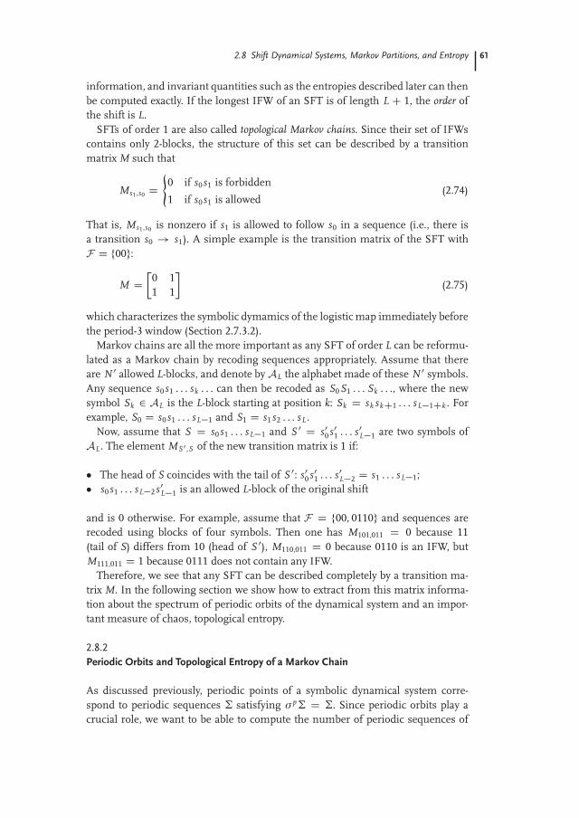
2.8 Shift Dynamical Systems, Markov Partitions, and Entropy 61
information, and invariant quantities such as the entropies described later can thenbe computed exactly. If the longest IFW of an SFT is of length L C 1, the order ofthe shift is L.
SFTs of order 1 are also called topological Markov chains. Since their set of IFWscontains only 2-blocks, the structure of this set can be described by a transitionmatrix M such that
Ms1,s0 D(
0 if s0s1 is forbidden
1 if s0s1 is allowed(2.74)
That is, Ms1,s0 is nonzero if s1 is allowed to follow s0 in a sequence (i.e., there isa transition s0 ! s1). A simple example is the transition matrix of the SFT withF D f00g:
M D
0 11 1
(2.75)
which characterizes the symbolic dymamics of the logistic map immediately beforethe period-3 window (Section 2.7.3.2).
Markov chains are all the more important as any SFT of order L can be reformu-lated as a Markov chain by recoding sequences appropriately. Assume that thereare N 0 allowed L-blocks, and denote by AL the alphabet made of these N 0 symbols.Any sequence s0 s1 . . . sk . . . can then be recoded as S0S1 . . . Sk . . ., where the newsymbol Sk 2 AL is the L-block starting at position k: Sk D sk skC1 . . . sL�1Ck . Forexample, S0 D s0 s1 . . . sL�1 and S1 D s1 s2 . . . sL.
Now, assume that S D s0 s1 . . . sL�1 and S 0 D s00 s0
1 . . . s0L�1 are two symbols of
AL. The element MS 0 ,S of the new transition matrix is 1 if:
The head of S coincides with the tail of S 0: s00 s0
1 . . . s0L�2 D s1 . . . sL�1;
s0 s1 . . . sL�2 s0L�1 is an allowed L-block of the original shift
and is 0 otherwise. For example, assume that F D f00, 0110g and sequences arerecoded using blocks of four symbols. Then one has M101,011 D 0 because 11(tail of S) differs from 10 (head of S 0), M110,011 D 0 because 0110 is an IFW, butM111,011 D 1 because 0111 does not contain any IFW.
Therefore, we see that any SFT can be described completely by a transition ma-trix M. In the following section we show how to extract from this matrix informa-tion about the spectrum of periodic orbits of the dynamical system and an impor-tant measure of chaos, topological entropy.
2.8.2
Periodic Orbits and Topological Entropy of a Markov Chain
As discussed previously, periodic points of a symbolic dynamical system corre-spond to periodic sequences Σ satisfying σ p Σ D Σ. Since periodic orbits play acrucial role, we want to be able to compute the number of periodic sequences of

62 2 Discrete Dynamical Systems: Maps
0 1
(a)
A
B
C(b)
Figure 2.17 A transition matrix can be repre-
sented by a directed graph. Nodes correspond
to possible states and edges indicate whether
transition from one state to another is possi-
ble. (a) This graph corresponds to transition
matrix (2.75); (b) this graph describes a gram-
mar in which C must be preceded by A: The
sequences BC and C C cannot occur.
period p of an arbitrary Markov chain, given its transition matrix M. This problemis part of a more general one, which is to determine the number of allowed symbolstrings of length n. An important measure of chaos, topological entropy, character-izes how this number increases when n ! 1.
A transition matrix is conveniently represented by a directed graph. To each sym-bol corresponds a node, which can be viewed as a state. When the transition from“state” i to “state” j is allowed (i.e., M j i ¤ 0), there is a directed edge going fromnode i to node j (Figure 2.17). The problems stated above can be reformulated asfollows: How many distinct paths of length n does the graph have? How many ofthese paths are closed?
We first compute the number P nj i of paths connecting node i to node j in exactly
n steps. This can be done inductively. Obviously, one can go from i to j in one steponly if there is an edge between the two sites, thus P1
j i D M j i . Then we note thateach itinerary linking i to j in n steps goes from i to some site k in n � 1 steps, thenfollows the edge from k to j in one step. By summing over all possible intermediarysites k, one obtains
P nj i D
NXkD0
M j k P n�1k i
which is immediately seen to be the rule for matrix multiplication. Since P1j i D
M j i , it follows that
P nj i D (M n) j i (2.76)
Hence all the relevant information is contained in the successive powers of thetransition matrix.

2.8 Shift Dynamical Systems, Markov Partitions, and Entropy 63
Periodic sequences of period p correspond to paths of length p that begin andend at the same node. Thus the number N f (p ) of periodic points of period p is
N f (p ) DN�1XkD0
M pk k D trM p (2.77)
Similarly, the number Ns(p ) of p-symbol strings equals the total number of pathsof length p � 1 and thus is given by the sum of the elements of M p�1. This canbe formalized as follows. Let V p be the vector whose ith component V p
i is thenumber of length-p symbol strings beginning with symbol i. It is easy to see thatthe components of V 1 are all 1 and that V p D M p�1V 1. Thus,
Ns(p ) D (V 1)T V p D (V 1)T M p�1V 1 (2.78)
Expressions (2.77) and (2.78) show that N f (p ) and Ns(p ) have the same asymp-totic behavior. Indeed, the action of M p for large p is determined by its largesteigenvalue λmax and the associated eigenvector. It is easily shown that if λmax > 1,then
limp!1
log N f (p )p
D limp!1
log Ns(p )p
D log λmax (2.79)
The growth rate of the number Ns(p ) of p-blocks
hT D limp!1
log Ns(p )p
D log λmax (2.80)
is called the topological entropy. It measures the average amount of informationthat is extracted by reading one symbol of a typical sequence. Equation 2.79 showsthat the topological entropy of a Markov chain depends in a very simple way onthe transition matrix. It also illustrates the fact that in general the growth rateof the number of periodic points is equal to the topological entropy, as noted inSection 2.6.4.1. More sophisticated techniques to compute topological entropy arepresented in Section 2.8.6. Let us consider two examples:
The eigenvalues of transition matrix (2.75) are (1 ˙ p5)/2. The largest one is
λmax � 1.618 033 9 and is known as the golden mean. This Markov chain, accord-ingly called the golden mean shift, has topological entropy hT � 0.481 211 8.
The transition matrix of the full N-shift is filled with 1s. Its largest eigenvalueis N, and the topogical entropy is hT D ln N . In particular, the 2-shift has hT D0.693 147 1, which is greater than for the golden mean shift: Topological entropyincreases as chaos becomes more developed.
2.8.3
Markov Partitions
Markov chains are interesting not only as model dynamical systems but also be-cause there are some classical dynamical systems whose symbolic dynamics can

64 2 Discrete Dynamical Systems: Maps
be represented exactly by a topological Markov chain. We have already encountereda few examples of such systems. The simplest ones are the tent and logistic mapsassociated with a full 2-shift: Every sequence of “0” and “1” is associated with aphysical orbit. The logistic map at the beginning of the period-3 window is anotherexample of a finite shift; the only forbidden sequence is the string “00.” A naturalquestion then is: Under what conditions is a dynamical system described faithfullyby a Markov chain?
The symbolic coding of a dynamical system relies on the existence of a parti-tion P D fP0,P1, . . . ,PN�1g of phase space into N disjoint regions Pi . At eachtime step, the current system state is coded with the symbol i associated with theregion Pi to which it belongs. Because the partition and the time-one map deter-mine completely the symbolic dynamics, it is not surprising that the condition forbeing describable by a Markov chain involves the partition and the images of themembers of the partition.
We now state this condition without a proof. Assume that there exists a partitionP D fPig such that the intersection of any member with the image of another iseither itself or empty:
8i, j Pi \ f�P j
� D(Pi
; (2.81)
The structure of such a partition can be described concisely but faithfully by a tran-sition matrix MP defined by
MPi j D
(1 if Pi \ f (P j ) ¤ ;0 otherwise
(2.82)
It can be shown that the dynamical system coded by the partition P is then com-pletely equivalent to the Markov chain of transition matrix MP . In particular, thetopological entropy of the original dynamical system is equal to that of the Markovchain, and both systems have the same spectrum of periodic orbits. According-ly, a partition P satisfying (2.81) is called a Markov partition. Examples of Markovpartitions in the logistic map at special values of parameter a are given in Sec-tion 2.9.2.
Note that even when there is a generating partition (such as the one based oncritical points of a one-dimensional map) and it is not of a Markov type, the exis-tence of a Markov partition is not precluded. If the system is equivalent to a shift ofa finite type, then an analysis of the symbolic dynamics obtained with the generat-ing partition should reveal that there are a finite number of irreducible forbiddenwords. As described in Section 2.8.1, a Markov chain can then be obtained with asuitable recoding and the topogical entropy computed using the associated transi-tion matrix.

2.8 Shift Dynamical Systems, Markov Partitions, and Entropy 65
2.8.4
Approximation by Markov Chains
In fact, only a small fraction of the regimes of a logistic map can be represented bya Markov chain exactly. Indeed, there is only a countable number of finite matricesof 0 and 1, whereas these regimes are indexed by parameter a, which is a realnumber [52]. Moreover, chaotic regimes are associated with kneading sequencesthat are not eventually periodic, which makes it generally impossible to describethe symbolic dynamics by a finite number of IFWs.
However, this does not make shifts of a finite type irrelevant. Indeed, it is notpossible to analyze arbitrarily long symbol sequences. In practice, there is an upperbound on the length of the longest symbolic sequence that can be obtained in areasonable time. This limits the search for forbidden symbol blocks to a maximallength. Otherwise, longer symbol blocks may be classified incorrectly as forbiddenonly because their probability of occurrence is too small. For example, assume thatan orbit of 1 million (� 220) points has been recorded and coded on two symbols. Itis certainly pointless to determine forbidden blocks longer than 20 symbols sincethe least probable one will occur at most once in the best case, where all blocks areequiprobable.
Therefore, Markov chains are still relevant for characterizing dynamical systemsthat are not conjugate to a shift of finite type, provided that a generating partitionis known and a long symbolic sequence has been recorded. If the list of forbiddenwords has been determined for word lengths up to L, this gives a natural approxi-mation of the system under study by a finite-type shift of order L, and hence by aMarkov chain after a suitable recoding. Note that this systematically overestimatestopological entropy estimates because higher-order forbidden sequences are ne-glected. The expression hT D ln λmax for a Markov chain assumes that the numberNs(p ) of p-blocks can be determined for arbitrary p from the transition matrix. Ifthere is more “pruning” than described by this transition matrix, the actual num-ber of sequences will be lower, as well as the topological entropy. Carrying out thiscomputation for increasing block lengths and comparing the results may help toestimate its accuracy.
2.8.5
Zeta Function
As shown in Section 2.8.2, the number of periodic points of period n, Pn , can becomputed as Pn D tr M n , where M is the Markov transition matrix. The infor-mation contained in the transition matrix can be transformed into a generatingfunction for Pn by defining
� (t) D exp
1X
nD1
Pn
nt n
!(2.83)
With a little bit of algebraic calisthenics, it is possible to show that
� (M, t) D 1det(Id � tM )
(2.84)

66 2 Discrete Dynamical Systems: Maps
We illustrate one use of the zeta function in the example below.
Example 2.2
The spectrum of orbits forced by the period-3 orbit 31 of the logistic map is com-puted using the Markov transition matrix M; cf. (2.75). If the matrices
Id D
1 00 1
and
M D
0 11 1
have been defined previously, as well as the positive integer N (D 12 below), thegenerating function
Pn Pn/nt n is given up to degree N by the simple Maple call
> taylor (�log (det(Id � t � M )) , t D 0, N C 1)
t C 32
t2 C 43
t3 C 74
t4 C 115
t5 C 186
t6 C 297
t7 C 478
t8 C 769
t9
C 12310
t10 C 19911
t11 C 32212
t12 C O �t13� (2.85)
We read these results as follows:
1. There is one period-1 point 11.2. There are three period-2 points. One is the period-1 point 11; the other two be-
long to the single period-2 orbit 21.3. There are four period-3 points. One is 11; the other three belong to the degenerate
saddle–node pair 31 (001 and 011).4. There are seven period-4 points, which belong to the orbits 11, 21, and 41 of the
initial period-doubling cascade.5. There are 11 period-5 points. One belongs to 11. The remaining 10 belong to
two period-5 orbits, which comprise the saddle–node pair 01111 and 01101.
Continuing in this way, we construct the remaining results. These are summarizedin Table 2.2. It is a simple matter to verify that the results of this table are consistentwith the results of Table 2.1 up to period 8.
2.8.6
Dealing with Grammars
At the saddle–node bifurcation of the period-3 orbit, the adjacency matrix (Markovtransition matrix) is given by (2.75). This matrix tells us that the symbol 0 mustbe followed by the symbol 1, and the symbol 1 can be followed by either of thesymbols 0 or 1.

2.8 Shift Dynamical Systems, Markov Partitions, and Entropy 67
Table 2.2 Number of orbits up to period p D 12 forced by 31 computed using the zeta function
based on the golden mean matrix (2.75).
p N(p ) Lower-period orbits Period-doubled Number of saddle–node pairs
1 1 11
2 3 (11C 21)
3 4 11 C 31
4 7 (11 C 21C 41) 05 11 11 1
6 18 11 C 21 C 31 17 29 11 2
8 47 (11 C 21 C 41 81) 2
9 76 11 C 31 410 123 11 C 21 C (51C 104) 5
11 199 11 9
12 322 (11 C 21 C 41) C 31 C (61C 122) 12
2.8.6.1 Simple Grammars
It is useful to introduce an alternative representation for the dynamics. This in-volves introducing two symbols (words) A D 01 and B D 1. These two words havelengths 2 and 1, respectively. In this representation, A can be followed by either Aor B, as is true also for B. The transition matrix is full:
M D
1 11 1
(2.86)
and the grammar is simple (no transitions are forbidden).The periodic orbits in the dynamics can be constructed as follows. Replace the
nonzero elements in the first row of M by the symbol A and those in the secondrow by the symbol B (A and B do not commute).
M D
1 11 1
�!
A AB B
D M (2.87)
Then the complete set of periodic orbits is constructed by computing trMn , n D1, 2, 3, . . .
Example 2.3
For n D 1, 2, and 3 we find
n tr Mn Orbits
1 A C B 01 C 1
2 2A2 C AB C B2 2(01)2 C 011 C (1)2
3 2A3 C 2ABA C 2A2 B C AB2 C B3 2(01)3 C 4(01101) C 0111 C (1)3

68 2 Discrete Dynamical Systems: Maps
Reduction to simple grammars is often useful in analyzing experimental da-ta. For example, chaotic data generated by the Belousov–Zhabotinskii reaction(cf. Chapter 7) have been reduced to a symbolic code sequence involving the twosymbols 0 and 1. The rules of grammar observed in the experimental data are asfollows:
1. The symbol 0 must be followed by the symbol 1.2. The symbol 1 can be followed by 0 or 1.3. Symbol sequences (11 � � � 1) of length p can occur for p D 1, 2, 3, 4 but not for
p > 4.
It appears that the vocabulary of this dynamics consists of the four words 01, 011,0111, and 01111. It also appears that any of these words can be followed by anyother word. The grammar is simple and represented by a 4 � 4 Markov transitionmatrix whose 16 elements are 1. The periodic orbits are obtained as described abovefor the golden mean case.
The topological entropy for dynamics consisting of a finite number of wordsof varying length obeying a simple grammar (full shift) is easily determined asfollows. Assume that there are w (p ) words of length p, p D 1, 2, 3, . . . Then thenumber of ways, N(T ), of constructing a word of length T is determined by thedifference equation
N(T ) D w (1)N(T � 1) C w (2)N(T � 2) C � � � DXpD1
w (p )N(T � p ) (2.88)
The number N(T ) behaves asymptotically like N(T ) � A(XM )T , where A is someconstant and XM is the largest real root of the characteristic equation
X T DXpD1
w (p )X T�p or 1 DXpD1
w (p )X p (2.89)
Example 2.4
For the full shift on two symbols 0 and 1,
1 D 2X
H) hT D log 2
Example 2.5
For golden mean dynamics, w (1) D 1, w (2) D 1, and
1 D 1X
C 1X 2 H) XM D 1 C p
52
and hT D 0.481 212

2.8 Shift Dynamical Systems, Markov Partitions, and Entropy 69
Example 2.6
For the Belousov data described above, w (p ) D 1 for p D 2, 3, 4, 5 and w (p ) D 0for p D 1 and p > 5, so that
1 D 1X 2
C 1X 3
C 1X 4
C 1X 5
XM D 1.534 158 and hT D 0.427 982
2.8.6.2 Complicated Grammars
There are many cases in which the dynamics either consists of or is well approx-imated by a finite vocabulary with a nontrivial grammar. The two questions ad-dressed above (description of periodic orbits, computation of entropy) are still ofinterest.
The spectrum of periodic orbits can be computed by following the algorithmused above.
1. Write out the Markov transition matrix M for the vocabulary.2. Replace each nonzero matrix element 1 in row i by the noncommuting symbol
wi representing the ith word, effecting the transition M ! M.3. Compute trMn for n D 1, 2, . . .4. Replace each word sequence by the appropriate sequence of symbols from the
original alphabet (i.e., 0 and 1).
The problem of computing the topological entropy for this dynamics is more sub-tle. It is isomorphic to the problem of computing the capacity of a transmissionchannel. The capacity of a transmission channel is (Shannon, [56, 57])
C D limT!1
1T
log N(T )
Here N(T ) is the number of allowed signals of duration T, and log is to base e.In many grammars, not all symbol sequences are allowed (qu is OK, qv is not).
In such cases, assume that there are m states b1, b2, . . . , bm. For each state onlycertain symbols from the set S1, S2, . . . , Sn can be transmitted (different subsetsfor different states). The transmission of symbol Sk from state bi to state b j (bi
may be the same as b j ) takes time t (k )i j , where k indexes all possible paths from bi
to b j . This process is illustrated by a graph such as that shown in Figure 2.17.
Theorem 2.1
The channel capacity C is log W0, where W0 is the largest real root of the m � mdeterminantal equationˇ
ˇXk
W �t(k)i j � δ i j
ˇˇ D 0 (2.90)
For our purposes, we can regard each state as a word and ti j is the length of word i.

70 2 Discrete Dynamical Systems: Maps
Example 2.7
Assume that the vocabulary has three words A, B, and C or w1, w2, and w3 oflengths p, q, and r and a grammar defined by Figure 2.17b. The Markov matrix is
M D241 1 1
1 1 01 1 0
35
The determinantal equation constructed from the Markov matrix and word lengthsis 2
6641
W p � 1 1W p
1W p
1W q
1W q � 1 0
1W r
1W r �1
3775 D 0
The characteristic equation for this dynamical system is
1W p C 1
W q C 1W pCr D 1
The topological entropy is hT D log W0, where W0 is the largest real eigenvalue ofthis characteristic equation.
2.9
Fingerprints of Periodic Orbits and Orbit Forcing
2.9.1
Permutation of Periodic Points as a Topological Invariant
Using kneading theory, periodic points with given symbolic itineraries can be or-dered along the interval. This is not only useful to determine the order in whichperiodic orbits appear but also to identify periodic orbits.
Indeed, consider the period-5 orbit with symbolic name 01011 of the logistic map(Figure 2.16). Its five periodic points are associated with the five cyclic permutationsof the symbolic name, ordered by kneading theory as follows:
01101 � 01011 � 11010 � 10101 � 10110 (2.91)
Label the sequences in (2.91) from left to right by Σ i , i D 1 . . . 5, and expressthem in terms of the leftmost sequence Σ1 D 01101 and of powers of the shiftoperator. We have
Σ1 � Σ2 D σ3Σ1 � Σ3 D σΣ1 � Σ4 D σ2Σ1 � Σ5 D σ4Σ1 (2.92)
We observe that under the action of the shift operator σ, these sequences are per-muted: The lowest sequence becomes the third, the second one the last, and so on.

2.9 Fingerprints of Periodic Orbits and Orbit Forcing 71
The corresponding permutation
π(01011) D (π i) D (3, 5, 4, 2, 1) (2.93)
such that σΣ i D Σπ i provides crucial information about the orbit. Its dynamicalrelevance owes much to two fundamental properties.
First, the permutation can be extracted directly from the periodic orbit without usingany symbolic encoding and without having the graph of the map. Indeed, consider theperiod-5 orbit in Figure 2.16. If we label the periodic points x1, x2, . . . , x5 fromleft to right, we can determine as above a permutation π such that f (xi ) D xπ i .Obviously, this permutation is identical to (2.93) (e.g., the image of the first pointis the third), which can easily be checked in Figure 2.16.
Second, permutation (2.93) remains identical on the entire domain of existence of theorbit in parameter space. As a parameter is varied, points xi of a periodic orbit movealong the interval, but they do so without ever becoming degenerate (otherwise,we would have one point with two images, in contradiction with the determinis-tic nature of the map). Thus the relative order of points is preserved, hence thecorresponding permutation.
An important attribute of this invariance property is that the permutations asso-ciated with orbits interacting in a bifurcation will be strongly related. For example,saddle–node partners will have identical permutations since they are indistinguish-able at the bifurcation. Similarly, the permutation associated with a period-doubledorbit can easily be obtained from that of its mother.
Since there is a definite relation between symbolic names and permutations onthe one hand, and periodic orbits and permutations on the other hand, we seethat the symbolic names of the orbits are more than a convenient labeling andthat they carry topological information. To illustrate this, we now show that in one-dimensional maps, much about the symbolic name of an orbit can be recoveredmerely from the permutation. Consider the graphical representation in Figure 2.18of permutation (2.93) extracted from Figure 2.16.
The global shape of Figure 2.18 is characteristic of unimodal permutations: Therelative order of the leftmost points is preserved, while that of the rightmost pointsis reversed (in particular, the rightmost point is mapped to the leftmost). This is asignature of the existence of branches with different parities in the underlying map(assumed unknown). In fact, Figure 2.18 can be viewed as a topological represen-tation of this map in a coordinate system where points xi are equidistant.
Let us note the orientation-preserving (resp. orientation-reversing) branch 0 (re-sp. 1). It can be seen from Figure 2.18 that x1 is necessarily on branch 0, while x3,x4, and x5 must be on branch 1. The coding of x2 is ambiguous: It can be on onebranch or the other without modifying the permutation. Taking into account thatthe orbit of x1 is x1 ! x3 ! x4 ! x2 ! x5, the symbolic name of this orbit isthus 0110
11 (i.e., any of the two saddle–node partners born in the 51 saddle–nodebifurcation listed in Table 2.1). If additional information is available, such as pari-ty (is the multiplier of the orbit positive or negative?), it is possible to distinguishbetween these two orbits.

72 2 Discrete Dynamical Systems: Maps
0
1
2
3
4
5
6
0 1 2 3 4 5 6
x n+
1
xn
Figure 2.18 Graphical representation (i, π i ) of permutation (2.93). Orientation-preserving and
orientation-reversing parts are easily distinguished.
By generalizing the example above, it is easy to see that every pair of saddle–node partners and every period-doubled orbit is associated with a different permu-tation. The permutation realized by a periodic orbit can thus be viewed as a genuinefingerprint of this orbit.
It is comforting to know that much of the discussion of this section is still rel-evant for orbits in three-dimensional flows. As discussed throughout this book,orbits in these systems will be associated with braids (a generalization of permuta-tions deeply linked to knot theory). These braids will be characterized by topologicalinvariants that do not depend on parameters and contain much information aboutthe symbolic dynamics and the genealogy of periodic orbits. Just as the structure ofunimodal maps governs that of the permutations (Figure 2.18), there is a system-atic way to study the global organization of braids in three-dimensional systems.
2.9.2
Topological Entropy of a Periodic Orbit
The permutation associated with a periodic orbit not only provides qualitative in-formation, but it can also provide estimates of fundamental quantitative measuresof chaotic dynamics, as we show next. The key idea is that if the underlying map iscontinuous, the way in which the points of the orbit are mapped onto each otherprovides information on orbits in an extended neighborhood of the orbit.
For simplicity, let us consider a superstable periodic orbit such as the period-5orbit of Figure 2.16. As previously, the points are numbered from left to right. Sincex2 is the critical point xc , the leftmost and rightmost points x1 and x5 correspondto the lower and upper bounds of the invariant interval I D [ f (xc), f 2(xc)] wherethe relevant dynamics is confined. Using the fact that the xi are mapped exactlyonto each other, this will allow us to build a topological model of the dynamics.
To this end, consider the following partition of the invariant interval I:
I D [x1, x5] D I1 [ I2 [ I3 [ I4 D [x1, x2] [ [x2, x3] [ [x3, x4] [ [x4, x5] (2.94)

2.9 Fingerprints of Periodic Orbits and Orbit Forcing 73
Using the interval arithmetics (2.53) and permutation (2.93), we find easily that
f (I1) D f ([x1, x2]) D [x3, x5] D I3 [ I4 (2.95a)
f (I2) D f ([x2, x3]) D [x4, x5] D I4 (2.95b)
f (I3) D f ([x3, x4]) D [x2, x4] D I2 [ I3 (2.95c)
f (I4) D f ([x4, x5]) D [x1, x2] D I1 (2.95d)
The set of relations (2.95) is the analog of relations f (I1) D f (I2) D I1 [ I2, whichcharacterize the surjective logistic and tent maps (note that in a complete descrip-tion of the map, the branch parities should also be specified). The key observationhere is that both sets of relations define Markov partitions. In the example above,the Markov transition matrix as defined in (2.82) reads
A D
2664
0 0 0 10 0 1 01 0 1 01 1 0 0
3775 (2.96)
where the nonzero entries correspond to pairs (Ii , I j ) such that Ii \ f (I j ) D Ii .Even though the regime under study corresponds to a superstable orbit, ma-trix (2.96) is a signature of a chaotic dynamics. Its largest eigenvalue is λmax �1.512 876 398, which yields a topological entropy of hT D ln λmax � 0.414 012 738 1.Moreover, the matrix is transitive, which indicates that the associated Markov chainis topologically mixing.
In fact, the topological entropy as computed above characterizes the periodic or-bit rather than the dynamical system to which it belongs: It is obtained from thepermutation associated to the orbit,4) not from the global structure of the system.However, the entire system cannot be less chaotic than implied by the periodicorbit. In particular, its topological entropy is necessarily greater than the entropyof the orbit. Thus, the observation of an orbit with a positive topological entropy(as obtained from its permutation), even in a window of stability, indicates thepresence of chaos in the system under study, and in particular the existence of aninfinity of periodic orbits. This is illustrated in the next section with the “period-3implies chaos” theorem. A similar statement will be made later for flows: Someperiodic orbits have knot types that can exist only in a chaotic system.
Note that the tools introduced here show why one-dimensional diffeomorphismsare not chaotic: Since they globally preserve or reverse the order of points, the asso-ciated transition matrices cannot have eigenvalues larger than 1. In fact, the readermay want to check that a one-dimensional diffeomorphism can only have a period-1 orbit, possibly a period-2 orbit if it globally reverses orientation.
4) For the sake of simplicity, we have indicated how to compute the topological entropy of an orbitonly at a special parameter value, where the orbit is superstable. However, the topological entropyof an orbit depends only on the permutation associated with it and should be considered as atopological invariant of the orbit, defined on its entire domain of existence.

74 2 Discrete Dynamical Systems: Maps
2.9.3
Period 3 Implies Chaos and Sarkovskii’s Theorem
To illustrate the discussion above, we present now the famous statement “period 3implies chaos,” according to which the presence in a map of the interval of a peri-odic orbit of period 3 forces the presence of orbits of any other period [58].
If we carry out the same calculation for the superstable 0011 orbit as for the 0110
11orbit in Section 2.9.2, we find a partition I D [ f 2(xc), xc ] [ [xc , f (xc)] whose tran-sition matrix is the golden mean matrix (2.75) that we have already encountered:
A GM D
0 11 1
(2.97)
It is easy to prove that 8n � 2, Ani i ¤ 0, hence there are fixed points for any period
p. This is our first example of the general fact that the existence of some periodicorbits can force the existence of many other (here, an infinity) periodic orbits. Thisphenomenon is usually referred to as orbit forcing.
Note that the Markov partitions constructed from superstable orbits are refine-ments of the partition used for symbolic codings since the critical point is one ofthe border points. As a result, the transition matrices contain all the informationneeded to determine whether a given symbolic name is admissible. The exampleof the period-3 orbit is particularly simple since the Markov partition coincideswith the coding partition: Transition matrix (2.97) indicates that all itineraries areallowed except those containing the string “00” (showing again that orbits of allperiods exist). One may check in Table 2.1 that this is indeed what distinguishesorbits born before the 31 saddle–node bifurcation from orbits created afterward.
That the existence of an orbit of period 3 implies the existence of orbits of anyother period can in fact be viewed as a particular case of a more general theoremdue to Sarkovskii [59] (see also [52]). Consider the following ordering of the naturalintegers, written as the product 2k � (2n C 1) of a power of 2 by a prime number:
2k � 1 C 2l � 1 (k < l) (2.98a)
2k � 1 C 2l � (2n C 1) (n > 0) (2.98b)
2l � (2n C 1) C 2k � (2n C 1) (k < l, n > 0) (2.98c)
2k � (2n C 1) C 2k � (2m C 1) (m < n) (2.98d)
For example,
1 C 2 C 22 C 23 C 24 � 7 C 24 � 3 C 22 � 5 C 22 � 3 C 2 � 3 C 7 C 5 C 3
Sarkovskii’s theorem states that if a continuous map of an interval into itself hasan orbit of lowest period p and q C p , it also has an orbit of lowest period q. It iseasily seen that (i) if there are infinitely many different periods in a map, all the

2.9 Fingerprints of Periodic Orbits and Orbit Forcing 75
periods corresponding to the period-doubling cascade of the period-1 orbit mustbe present; (2) since 3 comes last in (2.98), the presence of a period-3 orbit forcesorbits of all other periods as shown above. It can be verified that the succession ofbifurcations given in Table 2.1 satisfies the Sarkovskii theorem. In particular, thefirst period-7 orbit is created before the first period-5 orbit, which itself is createdbefore the period-3 orbit. Moreover, all even periods are present when the first oddperiod appears.
2.9.4
Period 3 Does Not Always Imply Chaos: Role of Phase-Space Topology
Since so many properties of unimodal maps hold at least approximately for higher-dimensional systems, it might be troubling that numerous apparent counterexam-ples to the “period 3 implies chaos” theorem can be found in physical systems. Inthe modulated CO2 lasers described in Chapter 1 and in Section 7.5.2, for example,it is quite common to observe multistability, with a period-3 orbit coexisting withthe initial period-1 orbit, no other periodic orbit being present. Thus, a period-3orbit does not necessarily imply chaos.
The clue to this paradox is that the modulated CO2 laser can be described bya three-dimensional flow, hence by a two-dimensional Poincaré map, while theSarkovskii theorem holds for a map of a one-dimensional interval into itself. Itturns out that phase-space topology has a dramatic influence on orbit forcing.
The key topological difference between the two geometries is that in the two-dimensional case, it is possible to connect each of the three periodic points ofthe period-3 orbit to any other without encountering the third one. In the one-dimensional case, the two extreme points are isolated by the middle one.
Therefore, the three periodic points must be considered as arranged along atopological circle (obviously, this also applies to maps of a circle into itself; seeSection 2.12). The three points divide this circle into three intervals versus two inthe one-dimensional case. When the map is applied, the three points are cyclicallypermuted and the three intervals accordingly exchanged. As a result, the associatedtransition matrix is a simple permutation matrix, with zero topological entropy. Theaction of the map on the periodic orbit is equivalent to a pure rotation, which doesnot itself imply the existence of a chaotic dynamics. However, although it appearsthat orbit forcing can be modified dramatically when the topology of phase space ischanged, it remains true in all cases that some orbits can force the existence of aninfinity of other orbits.
2.9.5
Permutations and Orbit Forcing
The statements of the Li–Yorke theorem and of the Sarkovskii theorem seem toimply that period is the fundamental property in implication chains among orbits.However, forcing relations are more fine-grained. Admittedly, the existence of aperiod-5 orbit forces the existence of at least a period-7 orbit. However, an orbit of

76 2 Discrete Dynamical Systems: Maps
the period-5 pair 51 of a logistic map does not force every period-7 orbit of this map.Actually, it forces the two 71 orbits but is forced by the two 72 orbits. As we will seebelow, it is in fact the permutation associated with a given orbit that determineswhich orbits it forces.
In Section 2.9.1, we noted that the permutation associated with a periodic orbitO could be represented graphically by a piecewise-linear map such as is shown inFigure 2.18. This map is conjugate to the Markov chain that describes the actionof the map on the periodic points of the orbit (Section 2.9.2). If the Markov chainhas positive topological entropy, it is chaotic, as is the piecewise-linear map, whichhas thus an infinite number of unstable periodic orbits. These orbits comprise theminimal set of orbits that must exist in a map having the original orbit O as one ofits periodic orbits. The existence of these orbits is forced by that of O.
As an example, we show that the period-5 orbit 01011 (born in bifurcation 71)forces exactly one pair of period-7 orbits and determines the symbolic code of thisorbit. To this end, we apply the techniques outlined in Section 2.8.6 to transitionmatrix (2.96). Using the noncommutative symbols I1, I2, I3, and I4, we first rewriteit as
A D
2664
0 0 0 I1
0 0 I2 0I3 0 I3 0I4 I4 0 0
3775 (2.99)
Then we compute
trA7 D [I1 I3 I3 I2 I4 I1 I4] C [I1 I3 I3 I3 I3 I2 I4] C (I3)7 (2.100)
where [W ] represents the n cyclic permutations of a length-n word W. The minimalmodel compatible with the period-5 orbit 01011 has thus two period-7 orbits, whoseitineraries in the Markov partition can be read from (2.100). Since interval I1 islocated to the left of the critical point (Section 2.9.2) and the intervals I2, . . . , I4
to the right of it, the canonical symbolic names of these orbits can be obtainedthrough the recoding I1 ! 0, fI2, I3, I4g ! 1. The two period-7 orbits forced bythe period-5 orbit under study are thus 0111101 and 0111101.
The reader can check in Table 2.1 that these are the two orbits born in saddle–node bifurcation 71 and that this bifurcation indeed occurs before 51 in the uni-versal sequence. By repeating the above calculation for all low-period orbits of thelogistic map, the whole universal sequence of Table 2.1 can be reproduced.
It is not a coincidence that the two period-7 orbits forced in the example aresaddle–node partners and thus are associated with the same permutation. As wassuggested by the simple example above, orbit forcing in one-dimensional maps isnaturally expressed as an order on permutations rather than on periods. This isillustrated in Section 9.3.1. In unimodal maps, each bifurcation corresponds to adifferent permutation (Section 2.9.1) so that this order on permutations induces atotal order on bifurcations, which corresponds to the universal sequence discussedin Section 2.7.5.3.

2.10 Two-Dimensional Dynamics: Smale’s Horseshoe 77
As is discussed in Chapter 9, there is no longer a total ordering of bifurcations intwo-dimensional maps (and three-dimensional flows). The topological structure ofa periodic orbit, then, is specified not by a permutation but by a braid type. Thereis a forcing relation on braid types. However, several saddle–node bifurcations canbe associated with the same braid type, so that the induced order on bifurcations isonly a partial order.
2.10
Two-Dimensional Dynamics: Smale’s Horseshoe
2.10.1
Horseshoe Map
While one-dimensional maps display the most distinctive features of deterministicchaos, they lack a crucial property of time-one maps or Poincaré maps of flows:They are not invertible, as are the equations describing flows. Because many phys-ical systems are described by differential equations, it is now time to turn to two-dimensional invertible maps to understand how the basic mechanisms studied inprevious sections can be embedded in an invertible dynamics. This is not a trivialproblem; many key points of our analysis of the tent and logistic map, such as prop-erty (2.31), rely heavily on noninvertibility. To help us in this task, our keystone willbe the two-dimensional analog of the tent map, the paradigmatic Smale horseshoe.
The tent map example makes it clear that a key ingredient of chaos is expansion,or stretching. Yet many experimental and numerical examples of chaotic systemsshow that for a large number of them (i.e., dissipative systems), the asymptoticdynamics is confined to a small region of state space. Thus expansion must be bal-anced by contraction, or squeezing, so that trajectories remain forever in a boundedregion. In continuous systems, these two antagonistic mechanisms can be com-bined by folding processes, as illustrated by Smale’s horseshoe map f S , defined asfollows.
Take the unit square S, stretch it along one direction (the unstable direction)by a factor of approximately 2, while squeezing it in the transverse direction (thestable direction). Then fold the deformed rectangle so that it occupies roughly thesame region as the original square, intersecting the latter in two disjoint strips(Figure 2.19a). Note that points located in the middle and the ends of S do notreturn to it.
The key topological property of the horseshoe map is that f (S ) \ S consists oftwo disjoint components:
f (S ) \ S D H0 [ H1 (2.101)
which are the two horizontal strips H0 and H1 shown in Figure 2.19a.To specify the action of the inverse map f �1, we only need to determine
f �1(H0 [ H1) since f �1( f (S ) \ S ) D S \ f �1(S ). As shown in Figure 2.19b,
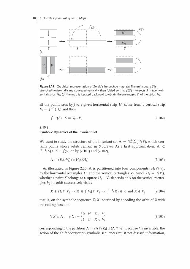
78 2 Discrete Dynamical Systems: Maps
S
f(S)fold
(a)
(b)
S S
S
H1
H0
0V V 1
Figure 2.19 Graphical representation of Smale’s horseshoe map. (a) The unit square S is
stretched horizontally and squeezed vertically, then folded so that f (S) intersects S in two hori-
zontal strips Hi ; (b) the map is iterated backward to obtain the preimages Vi of the strips Hi .
all the points sent by f to a given horizontal strip Hi come from a vertical stripVi D f �1(Hi ) and thus
f �1(S )\S D V0[V1 (2.102)
2.10.2
Symbolic Dynamics of the Invariant Set
We want to study the structure of the invariant set Λ D \C1�1 f n(S ), which con-
tains points whose orbits remain in S forever. As a first approximation, Λ f �1(S ) \ S \ f (S ) or, by (2.101) and (2.102),
Λ (V0[V1) \ (H0[H1) (2.103)
As illustrated in Figure 2.20, Λ is partitioned into four components, Hi \ Vj ,by the horizontal rectangles Hi and the vertical rectangles Vj . Since Hi D f (Vi ),whether a point X belongs to a square Hi \ Vj depends only on the vertical rectan-gles Vj its orbit successively visits:
X 2 Hi \ Vj , X 2 f (Vi ) \ Vj , f �1(X ) 2 Vi and X 2 Vj (2.104)
that is, on the symbolic sequence Σ(X ) obtained by encoding the orbit of X withthe coding function
8X 2 Λ , s(X ) D(
0 if X 2 V0
1 if X 2 V1(2.105)
corresponding to the partition Λ D (Λ \ V0) [ (Λ \ V1). Because f is invertible, theaction of the shift operator on symbolic sequences must not discard information,

2.10 Two-Dimensional Dynamics: Smale’s Horseshoe 79
0.0 0.1
1.0 1.1H1
H0
0V V1
Figure 2.20 The invariant set Λ is contained in the intersec-
tions of the vertical rectangles Vi with the horizontal rectangles
Hi . As explained in the text, Hi \ Vj is labeled i. j .
unlike in the one-dimensional case. Thus the sequence Σ(X ) associated to X mustbe bi-infinite:
Σ(X ) D . . . s�3 s�2 s�1.s0 s1 s2 . . . s i D s( f i(X )) i 2 Z (2.106)
with the dot separating the forward sequence ΣC(X ) D s0 s1 . . . from the backwardsequence Σ�(X ) D s�1s�2 . . . These two sequences describe the future and the pastof the point, respectively. Applying the shift operator to a sequence simply amountsto shifting the dot: σ(. . . s�1.s0 s1 . . .) D . . . s�1s0.s1 . . .
As in (2.46), let us define cylinders as sets of points whose symbolic sequencescontain a common substring, such as
C [s�2s�1.s0 s1] � fX 2 ΛI Σ(X ) D . . . s�2 s�1.s0 s1 . . .g (2.107)
It is easily seen from (2.104) that the squares in Figure 2.20 are cylinders:
�Hi \ Vj
� \ Λ D C[i. j ] (2.108)
which explains the labeling of the squares in Figure 2.20. To show that the partitionbased on (2.105) is generating, we now detail the structure of Λ and of higher-ordercylinders.
Start from the cylinders C[i. j ] D Hi \ Vj shown in Figures 2.20 and 2.21aand compute their images C[i j.] D f (C[i. j ]). These are the horizontal rectan-gles Hi j D f (Hi ) \ H j shown in Figure 2.21b, which are seen to be the com-ponents of f 2(S ) \ S . A dual decomposition of Λ is based on the preimagesC[.i j ] D f �1(C[i. j ]), which are the vertical rectangles Vi j D Vi \ f �1(Vj ) cov-ering f �2(S ) \ S (Figure 2.21c).
Figure 2.21d illustrates the fact that the four-symbol cylinders C[i j.k l ] can be ob-tained as the intersections of the vertical and the horizontal two-symbol rectangles:
C[i j.k l ] D C[i j.]\C[.k l ] D Hi j \Vk l D f 2(Vi)\ f (Vj )\Vk\ f �1(Vl ) (2.109)
which follows directly from definition (2.108). The forward (resp. backward) se-quence ΣC(X ) (resp. Σ�(X )) specifies in which of the vertical (resp. horizontal)rectangles Vi j (resp. Hi j ) point X lies.
Note that if one takes into account that Σ�(X ) D s�1 s�2 . . . should be read fromthe labels of Figure 2.21b from right to left, forward and backward sequences are

80 2 Discrete Dynamical Systems: Maps
01.01 01.11
11.00 11.01 11.11 11.10
01.10
10.00 10.01 10.11 10.10
00.00 00.01 00.11 00.10
(b)
(a) (c)
(d)
01.00
0.10.0
1.0 1.1
.00 .01 .11 .10
11.
01.
10.
00.
Figure 2.21 (a) Decomposition of f (S) \ S \f �1(S) in squares Hi \Vj . These are mapped
by the horseshoe map f to (b) the horizontal
rectangles Hi j D f (Hi ) \ H j , which are
the components of f 2(S) \ S , and by f �1 to
(c) the vertical rectangles Vi j D Vi \ f �1(Vj ),
which cover f �2(S) \ S . Arrows indicate the
action of the horseshoe map; (d) by intersect-
ing the horizontal with the vertical rectangles,
one obtains a cover of the invariant set Λ by
cylinders C[i j.k l].
ordered in exactly the same way along the horizontal and vertical sides of S, re-spectively. In fact, they follow the unimodal order that governs the tent and logisticmaps: This is a signature of the folding process (cf. Figure 2.14).
In general, cylinders of the type C[s�N . . . s�1.s0 . . . sN�1] will be contained inthe 22N intersections of 2N vertical rectangles with 2N horizontal rectangles. With-out loss of generality, the action of the horseshoe map can be chosen to be piece-wise linear in the regions of interest, with expansion and contraction rates λu > 2and λ s < 1/2. In that case, the vertical rectangles Vs0...sN�1 will be of width 1/λN
uwhile the height of the horizontal rectangles Hs�N ...s�1 will be λN
s . It is easy to seethat both sizes shrink to zero in the limit N ! 1, and thus that the cylinderC[s�N . . . s�1.s0 . . . sN�1] converges to a unique point, as required for a generatingpartition.
This shows that the invariant set Λ is the product of a Cantor set of vertical lineswith a Cantor set of horizontal lines, and that it is in 1 W 1 correspondence withthe set of bi-infinite binary sequences. It can even be shown that this correspon-dence is a homeomorphism if the space of symbolic sequences is equipped withthe following metric:
d�fskgk2Z,
˚s0
k
�k2Z
� D1X
iD�1
δ i
2jijδ i D
(0 if s i D s0
i
1 if s i ¤ s0i
(2.110)

2.10 Two-Dimensional Dynamics: Smale’s Horseshoe 81
which means that the closer two sequences are according to this metric, the closerthe associated points are. This property will be useful in what follows.
2.10.3
Dynamical Properties
A few dynamical properties of the horseshoe map can be deduced from the discus-sion of previous sections. Some of them follow directly from the correspondencewith a full shift, as discussed in Section 2.6.5: sensitivity to initial conditions, exis-tence of a dense set of periodic orbits, existence of dense orbits, and so on. Othersare linked to the coexistence of two complementary mechanisms, stretching andsqueezing, and to the horseshoe map’s being two-dimensional. In particular, a fo-liation of Λ can be constructed in the following way.
Consider a point X and the vertical line V(X ) passing through X. From the resultsof Section 2.10.2 it is easy to see that X and any point Y 2 V(X ) have the sameforward sequence ΣC(X ) D ΣC(Y ) (the vertical line is the limit of a sequence ofvertical rectangles). This implies that X and Y have the same future, more preciselythat their orbits converge to each other in forward time: d( f n(X ), f n(Y )) ! 0 asn ! 1. Indeed, the two corresponding symbolic sequences converge to each otheraccording to metric (2.110) as the discrepancies between them are pushed fartherand farther in the backward sequence.
Let us define the stable and unstable manifolds Ws(X ) and Wu(X ) of a point Xas the sets of points whose orbits converge to that of X in the future and in the past,respectively:
Ws(X ) Dn
Y 2 Λ , limn!1
d ( f n(X ), f n(Y )) D 0o
(2.111a)
Wu(X ) Dn
Y 2 Λ , limn!1
d ( f �n(X ), f �n(Y )) D 0o
(2.111b)
According to this definition, the vertical line V(X ) is a segment of the stable mani-fold of X: V(X ) Ws(X ).
Similarly, two points X 0 and Y 0 located along the same horizontal line H(X 0)have the same backward sequence, hence the same past. Their orbits converge toeach other backward in time: d( f �n(X 0), f �n(Y 0)) ! 0 as n ! 1. Thus theybelong to the same segment of unstable manifold Wu(X 0) D Wu(Y 0).
Hence Λ is foliated by horizontal and vertical lines that are segments of stableand unstable manifolds, respectively. The astute reader may have noticed that thiscould have been obtained directly from the geometrical description of the horse-shoe map. However, it is in general not straightforward to determine these seg-ments for a general two-dimensional invertible map. Because the discussion aboveis based on symbolic dynamical properties only, it can be extended directly to alarge class of dynamical systems: As soon as a symbolic encoding of the invari-ant set is available, segments of stable and unstable manifolds can be obtainedsimply by following points with identical forward or backward sequences, respec-tively.

82 2 Discrete Dynamical Systems: Maps
We conclude this section with an important remark regarding how noninvertibil-ity can be embedded in an invertible dynamics. As discussed above, each verticalline V is associated with a unique forward sequence ΣC(V) shared by all the pointsin the line. Obviously, the images of all these points will have the same forwardsequence: The image of the line by the horseshoe map is thus another vertical linef (V) whose forward sequence is ΣC( f (V)) D σΣC(V).
If V(Λ) represents the complete set of vertical lines (or, equivalently, of class-es of points with identical forward sequences), the horseshoe map induces a mapf V W V(Λ) ! V(Λ). Because forward sequences are one-sided, map f V is intrin-
sically noninvertible; in fact, it is conjugate to the tent map since we know thatforward sequences are ordered according to the unimodal order. In the invertiblehorseshoe map, there is thus an underlying noninvertible map that organizes the dy-namics.
The clue to this paradox is that the shift operator acts on symbol sequences bytransferring one symbol from the forward sequence to the backward sequence. Theforward sequence loses information (i.e., the associated dynamics is noninvertible),gained by the backward sequence (whose dynamics thus depends on the forwardsequence), while the net information flow is zero for the complete sequence (i.e.,the global dynamics is invertible). Again, we see that this observation applies to alarge class of dynamical systems, and it will be one of the building blocks of thisbook.
To conclude, let us emphasize that the two-sidedness of symbolic sequences forthe horseshoe map is not due directly to the dynamics’ being two-dimensional.Rather, it originates in the distinction between stable and unstable subspaces, re-gardless of their dimension. For example, one could imagine that forward (resp.backward) sequences parameterize a two (resp. one)-dimensional subspace.
2.10.4
Variations on the Horseshoe Map: Baker Maps
The tent map is the simplest one-dimensional map that is conjugate to a fullone-sided 2-shift. To illustrate horseshoe dynamics, we now present examples ofpiecewise-linear maps that are conjugate to two-sided full shifts. These maps arethe two-dimensional counterparts of the tent map. As we shall see, the stretchingand squeezing mechanisms at play in the horseshoe map can be organized in afew inequivalent ways.
For definiteness, we restrict ourselves to bijections of the unit square into itself.Our first example, shown in Figure 2.22a, is a deformation of the horseshoe mapof Figure 2.19. It is easily seen that this map can be described by two linear mapsdefined on the domains x < 1/2 and x > 1/2. More precisely, the coordinates(x 0, y 0) of the image of a point (x , y ) are given by
x 0 D 1 � 2ˇˇx � 1
2
ˇˇ , y 0 D
(y 0
2 if x � 12
1 � y 0
2 if x > 12
(2.112)

2.10 Two-Dimensional Dynamics: Smale’s Horseshoe 83
A
B
A B
A B
A B
BA
B
A
(a)
(b)x
x
y
y
y
y
x
x0
0
0
0
Figure 2.22 Two topologically distinct horseshoelike maps that differ in the folding process.
Rotation of rectangle B can occur in the (a) counterclockwise or in the (b) clockwise directions.
Note that while the one-dimensional tent map is continuous but not differentiableat the critical point, the two-dimensional piecewise-linear map (2.112) has neces-sarily a discontinuity, here at the line x D 1/2. More importantly, (2.112) are ourfirst example of a reducible system. Indeed, they have the following structure:
x 0 D f (x ) (2.113a)
y 0 D g(x , y ) (2.113b)
The key property of (2.113) is that it has a lower-dimensional subsystem (2.113a)that can be iterated independently: The dynamics of the x variable depends onlyon x itself. From the discussion of previous sections, this is not surprising. Indeed,the y direction is the stable direction, and vertical lines x D c are segments of thestable manifold. Since the vertical lines parameterized by x are mapped to othervertical lines, the original two-dimensional map induces a one-dimensional mapx 0 D f (x ). As discussed earlier, this map is intrinsically noninvertible: An invert-ible chaotic dynamics in the global state space is associated with a noninvertibledynamics in the unstable space.
This structure allows one to represent the action of map (2.112) by plotting thegraphs (x , x 0) and (y , y 0), as shown in Figure 2.23. We see that the chaotic two-dimensional map (2.112) is associated with two singular one-dimensional maps( f u, f s ) such that x 0 D f u(x ) and y D f s(y 0). The existence of f u has been dis-cussed previously and is a signature of the folding process. The existence of f s
follows from the fact that map (2.112) is invertible and that for the inverse map,stable and unstable spaces are exchanged. Hence the inverse map is associatedwith one-dimensional maps ( f s , f u). Note that f s is not arbitrary: Each monotonicbranch of f s corresponds to a given branch of f u. Therefore, both maps have thesame number of branches.
Figures 2.22b and 2.23b display another map that is extremely similar to our firstexample, except that folding takes place in the other direction. We note that the two

84 2 Discrete Dynamical Systems: Maps
0
0.2
0.4
0.6
0.8
1
0 0.2 0.4 0.6 0.8 1
x'
x
0
0.2
0.4
0.6
0.8
1
0 0.2 0.4 0.6 0.8 1
y'
y(b)
0
0.2
0.4
0.6
0.8
1
0 0.2 0.4 0.6 0.8 1
x'
x
0
0.2
0.4
0.6
0.8
1
0 0.2 0.4 0.6 0.8 1
y'
y(a)
Figure 2.23 Graphs of the noninvertible one-dimensional maps associated with the invertible
maps of Figure 2.22; (a) corresponds to the map in Figure 2.22a and (b) corresponds to the
map in Figure 2.22b.
maps are associated with the same map in the unstable space, but not in the stablespace. They are topologically distinct. These two topologically classes will later bereferred to as the horseshoe and the reverse (or twisted) horseshoe. We shall see inChapter 7 that both classes can be observed experimentally.
In these examples, reducibility is clearly apparent because the unstable and sta-ble directions are fixed over the state space. This makes it easy to find coordinatesystems whose axes are parallel to these directions. As the example of the Hénonmap in the next section will show, this is not the case in general. However, it istempting to conjecture that the equations describing a chaotic system can alwaysbe brought, at least approximately, to a reducible form (2.113) by a suitable changeof coordinates. As noted previously, this should be the case if a good symbolic de-scription of the system is available: Points that have identical forward (resp. back-
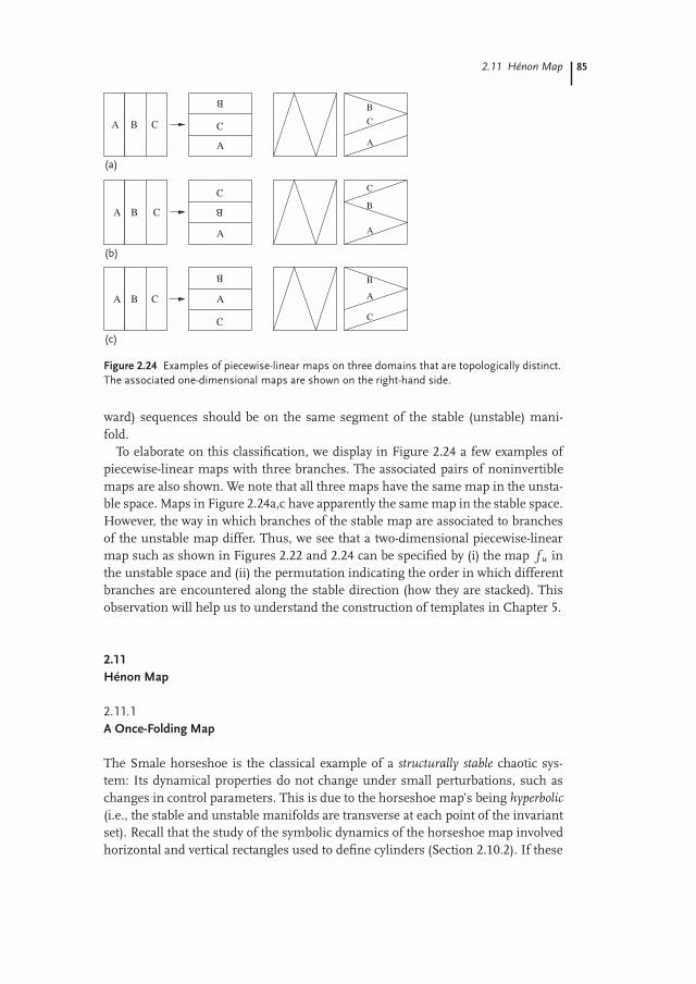
2.11 Hénon Map 85
A B C
A B C
A B C
B
C
A
A
C
B
A
C
B
C
A
B
A
B
C
A
C
B
(a)
(b)
(c)
Figure 2.24 Examples of piecewise-linear maps on three domains that are topologically distinct.
The associated one-dimensional maps are shown on the right-hand side.
ward) sequences should be on the same segment of the stable (unstable) mani-fold.
To elaborate on this classification, we display in Figure 2.24 a few examples ofpiecewise-linear maps with three branches. The associated pairs of noninvertiblemaps are also shown. We note that all three maps have the same map in the unsta-ble space. Maps in Figure 2.24a,c have apparently the same map in the stable space.However, the way in which branches of the stable map are associated to branchesof the unstable map differ. Thus, we see that a two-dimensional piecewise-linearmap such as shown in Figures 2.22 and 2.24 can be specified by (i) the map f u inthe unstable space and (ii) the permutation indicating the order in which differentbranches are encountered along the stable direction (how they are stacked). Thisobservation will help us to understand the construction of templates in Chapter 5.
2.11
Hénon Map
2.11.1
A Once-Folding Map
The Smale horseshoe is the classical example of a structurally stable chaotic sys-tem: Its dynamical properties do not change under small perturbations, such aschanges in control parameters. This is due to the horseshoe map’s being hyperbolic(i.e., the stable and unstable manifolds are transverse at each point of the invariantset). Recall that the study of the symbolic dynamics of the horseshoe map involvedhorizontal and vertical rectangles used to define cylinders (Section 2.10.2). If these
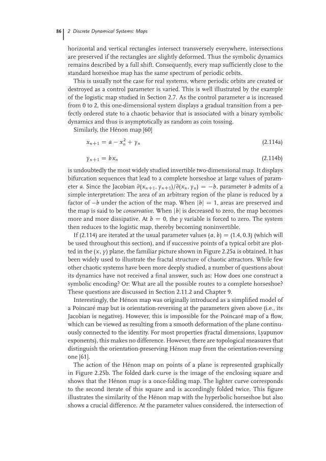
86 2 Discrete Dynamical Systems: Maps
horizontal and vertical rectangles intersect transversely everywhere, intersectionsare preserved if the rectangles are slightly deformed. Thus the symbolic dynamicsremains described by a full shift. Consequently, every map sufficiently close to thestandard horseshoe map has the same spectrum of periodic orbits.
This is usually not the case for real systems, where periodic orbits are created ordestroyed as a control parameter is varied. This is well illustrated by the exampleof the logistic map studied in Section 2.7. As the control parameter a is increasedfrom 0 to 2, this one-dimensional system displays a gradual transition from a per-fectly ordered state to a chaotic behavior that is associated with a binary symbolicdynamics and thus is asymptotically as random as coin tossing.
Similarly, the Hénon map [60]
xnC1 D a � x2n C yn (2.114a)
ynC1 D bxn (2.114b)
is undoubtedly the most widely studied invertible two-dimensional map. It displaysbifurcation sequences that lead to a complete horseshoe at large values of param-eter a. Since the Jacobian @(xnC1, ynC1)/@(xn , yn) D �b, parameter b admits of asimple interpretation: The area of an arbitrary region of the plane is reduced by afactor of �b under the action of the map. When jbj D 1, areas are preserved andthe map is said to be conservative. When jbj is decreased to zero, the map becomesmore and more dissipative. At b D 0, the y variable is forced to zero. The systemthen reduces to the logistic map, thereby becoming noninvertible.
If (2.114) are iterated at the usual parameter values (a, b) D (1.4, 0.3) (which willbe used throughout this section), and if successive points of a typical orbit are plot-ted in the (x , y ) plane, the familiar picture shown in Figure 2.25a is obtained. It hasbeen widely used to illustrate the fractal structure of chaotic attractors. While fewother chaotic systems have been more deeply studied, a number of questions aboutits dynamics have not received a final answer, such as: How does one construct asymbolic encoding? Or: What are all the possible routes to a complete horseshoe?These questions are discussed in Section 2.11.2 and Chapter 9.
Interestingly, the Hénon map was originally introduced as a simplified model ofa Poincaré map but is orientation-reversing at the parameters given above (i.e., itsJacobian is negative). However, this is impossible for the Poincaré map of a flow,which can be viewed as resulting from a smooth deformation of the plane continu-ously connected to the identity. For most properties (fractal dimensions, Lyapunovexponents), this makes no difference. However, there are topological measures thatdistinguish the orientation-preserving Hénon map from the orientation-reversingone [61].
The action of the Hénon map on points of a plane is represented graphicallyin Figure 2.25b. The folded dark curve is the image of the enclosing square andshows that the Hénon map is a once-folding map. The lighter curve correspondsto the second iterate of this square and is accordingly folded twice. This figureillustrates the similarity of the Hénon map with the hyperbolic horseshoe but alsoshows a crucial difference. At the parameter values considered, the intersection of

2.11 Hénon Map 87
-0.6
-0.4
-0.2
0
0.2
0.4
0.6
-2 -1.5 -1 -0.5 0 0.5 1 1.5 2
y
x
-0.6
-0.4
-0.2
0
0.2
0.4
0.6
-2 -1.5 -1 -0.5 0 0.5 1 1.5 2
y
x(a) (b)
Figure 2.25 (a) The Hénon attractor obtained with (2.114) for a D 1.4, b D 0.3; (b) to illustrate
the action of the map, the first and second iterates of the square [�2, 2] � [�0.6, 0.6] have been
plotted, showing that the Hénon map is a once-folding map.
the square enclosing the invariant set and of its image is in one piece, whereas ithad two disjoint components in the case of the horseshoe map (Figure 2.19).
Since this natural partition of state space in two regions was the keystone of ourstudy of the symbolic dynamics of the horseshoe map, it is not obvious whetherthere is a symbolic coding for the Hénon map and how it can be constructed.We discuss this important question in Section 2.11.2. We shall see that it is di-rectly connected to the nonhyperbolicity of the Hénon attractor (i.e., to the lackof transversality of certain intersections between the stable and unstable mani-folds).
2.11.2
Symbolic Dynamics of the Hénon Map: Coding
The relevance of symbolic codings relies heavily on the mixing property of chaoticdynamics (Section 2.7.2). Assume that we have an arbitrary partition M D M1 [M2
of phase space. If a map f is mixing, there exists for any region N 2 M an integern0(M ) such that f n0 (N )\M1 ¤ ; and f n0 (N )\M2 ¤ ;. However small a region Nis, there exist points in N with different symbolic itineraries, and thus N can alwaysbe divided into smaller regions. Since this operation can in principle be repeatedindefinitely, it could be tempting to believe that well-defined symbolic codings existfor any choice of the partition.
However, the example of the logistic map in Section 2.7 has shown that this is nottrue. The weakness in the argument above is that mixing cannot be invoked if theorbits of two points are strongly correlated for arbitrarily long times. In particular,we noted in our study of the logistic map that the different preimages of a givenpoint must be associated with different symbols. This rule is indeed necessary toprevent the symbolic itineraries of such points from being identical since theirorbits differ only in their initial conditions. If the map under study is expansive,

88 2 Discrete Dynamical Systems: Maps
separating preimages is actually sufficient for obtaining generating partitions, aswas shown in Section 2.7.2.
However, this criterion cannot be applied to the Hénon map; since it is invertible,every point has one and only one preimage. Thus we have to extend the simplerule used for the logistic map to handle the case of invertible chaotic maps. Theextension should also be consistent with the coding of the hyperbolic horseshoemap.
The key point is that while the orbits of two different points cannot collapse ontoeach other in finite time if the map is invertible, they can become indiscernible afteran infinite number of iterations: Two different points can have the same asymptoticfuture or the same asymptotic past (or both), as we see below.
In Figure 2.26a, we have plotted segments of the local stable and unstable mani-folds of the fixed point X � � (0.884, 0.265). We denote these segments by W l
s andW l
u , respectively. Recall that the stable manifold Ws(X �) and unstable manifoldWu(X �) consist of the points whose orbits converge to the fixed point X � underrepeated action of the Hénon map f and of the inverse map f �1, respectively:
X 2 Ws(X �) , limn!C1
jj f n(X ) � X �jj D 0 (2.115a)
X 2 Wu(X �) , limn!C1
jj f �n(X ) � X �jj D 0 (2.115b)
Obviously, the stable and unstable manifolds are invariant under both f and f �1,hence the restrictions of these maps to the invariant manifolds behave like one-dimensional diffeomorphisms. Since the eigenvalues of the Jacobian at X � alongthe stable and unstable directions are 0.156 > 0 and �1.92 < 0, f and f �1 preserve(reverse) orientation along the stable (unstable) manifold. The action of f �1 onthe stable segment W l
s and that of f on the unstable segment W lu are illustrated
in Figure 2.26b–f, which display f �n(W ls )) and f n(W l
u) for n D 1, 2, 3, 4, and 8,respectively. The two segments are stretched at each step and span a longer andlonger part of the two invariant manifolds.5) They are also folded at each iteration,a signature of the horseshoelike process that organizes the Hénon attractor. Forexample, Figure 2.26c can be compared with Figure 2.21 (keeping in mind that,unlike the classical horseshoe map, the Hénon map is orientation-reversing alongthe unstable manifold).
An extremely important consequence of the folding mechanism is that the stableand unstable manifolds of the fixed point X � intersect themselves not only at X �
but also at other locations, called homoclinic points. Since homoclinic points belongto both the unstable and the stable manifolds, their orbits converge to the fixedpoint both forward and backward in time. The stable and unstable manifolds beinginvariant, the set of homoclinic points is itself invariant: All images and preim-ages of a homoclinic point are themselves homoclinic points. More generally, twopoints are said to be homoclinic to each other if their orbits converge to each other
5) This is how segments W ls and W l
u of this example were themselves obtained, by iteratingrepeatedly from extremely small linear segments located around the fixed points and alignedalong the stable and unstable direction at that point.

2.11 Hénon Map 89
-0.6
-0.4
-0.2
0
0.2
0.4
0.6
-2 -1.5 -1 -0.5 0 0.5 1 1.5 2
y
x
-0.6
-0.4
-0.2
0
0.2
0.4
0.6
-2 -1.5 -1 -0.5 0 0.5 1 1.5 2
y
x
-0.6
-0.4
-0.2
0
0.2
0.4
0.6
-2 -1.5 -1 -0.5 0 0.5 1 1.5 2
y
x
-0.6
-0.4
-0.2
0
0.2
0.4
0.6
-2 -1.5 -1 -0.5 0 0.5 1 1.5 2
y
x
-0.6
-0.4
-0.2
0
0.2
0.4
0.6
-2 -1.5 -1 -0.5 0 0.5 1 1.5 2
y
x
-0.6
-0.4
-0.2
0
0.2
0.4
0.6
-2 -1.5 -1 -0.5 0 0.5 1 1.5 2
y
x
(a) (b)
(c) (d)
(e) (f)
X*
X* X*
f−2(P)
f −3 (P)
f 2(P)
X*
f 3(P) f−4 (P)
X*
f −1 (P)
f(P)
P
Figure 2.26 (a) The solid (dotted) line rep-
resents a segment W lu (W l
s ) of the unstable
(stable) manifold of the fixed point located
at their intersection. The orbits of points be-
longing to this line converge to the fixed point
backward (forward) in time; (b–e) images
f n (W lu ) and preimages f �n (W l
s ) of the seg-
ments W lu and W l
s for n D 1, 2, 3, 4. They
are folded at each iteration and the number
of intersections grows exponentially; (f) this
is the same picture after eight iterations. The
image of the unstable segment becomes in-
discernible from the strange attractor. One
clearly notices locations where the stable and
unstable manifolds are tangent. These de-
generate intersections are called homoclinic
tangencies.

90 2 Discrete Dynamical Systems: Maps
both forward and backward in time, with “homoclinic points” denoting points thatare homoclinic to a fixed point. The loop formed by the pieces of the stable andunstable manifolds joining X � and P is called a homoclinic loop.
Figure 2.26 also shows that, since the segments f �n(W ls ) and f n(W l
u) are in-creasingly folded as the iteration number n increases, the number of intersectionsNi(n) between the two segments (and thus of apparent homoclinic points) increas-es exponentially with n. However, it does not grow as fast as could have been expect-ed from the study of the horseshoe map: Ni (1) D 4, Ni (2) D 12 and Ni (3) D 30instead of Ni (n) D 4n for the horseshoe. This is an indication that the symbolicdynamics is not described by a full 2-shift.
In Figure 2.26b, we have distinguished two of the three homoclinic pointspresent at that stage. By studying how f and f �1 act on the segments shownin Figure 2.26a,b, it is easy to see that one point, denoted by P, is the image ofthe other, indicated as f �1(P ). Images and preimages of P are easily located inFigure 2.26b–e. Since they are themselves homoclinic points, they can be foundamong the intersections that appear in the consecutive plots of Figure 2.26. Forexample, P D W l
s \ ( f (W lu ) n W l
u ), hence f (P ) 2 W ls \ ( f 2(W l
u) n f (W lu )), which
consists of two points. These two points are the images of P and of the unlabeledhomoclinic point shown in Figure 2.26b. Since the latter is further from X � than Pand since f is continuous, f (P ) is the point of W l
s \( f 2(W lu)n f (W l
u )) that is closestto X � (Figure 2.26c). Determining the positions of all the images and preimagesf i (P ) shown in Figure 2.26b–e is an interesting exercise left to the reader.
We see that the sequence fP, f (P ), f 2(P ), f 3(P ), . . .g converges to the fixed pointX � along the stable manifold, approaching it from one side. Similarly, the se-quence fP, f �1(P ), f �2(P ), f �3(P ), . . .g converges to the fixed point along theunstable manifold, alternating between the two sides of the fixed point and witha smaller convergence rate since the unstable eigenvalue is negative and has amodulus closer to one than the stable eigenvalue. Thus, the orbits of X � and P arestrongly correlated both in the past and in the future, and some care has to be takenin order to prevent the two points from being associated with the same symbolicitinerary.
Before addressing this problem, a few remarks are in order. First, we note thatthe existence of homoclinic points forces the unstable manifold to be infinitelyfolded. On the one hand, all the f i (P ) iterates belong to the unstable manifold,by definition. On the other hand, it can be seen in Figure 2.26b–e that they allbelong for i > 0 to the segment of the stable manifold joining P and X � (f iscontracting along the stable manifold). Thus, the unstable manifold intersects thissegment infinitely many times and is infinitely folded, which is consistent withwhat Figure 2.26 shows. The same argument can be applied to the stable manifold.This suggests that homoclinic points are associated with a complicated dynamics.As a matter of fact, it can be proven that if a dynamical system displays homoclinicpoints, then it has an invariant set on which the dynamics is chaotic and there areperiodic orbits arbitrarily close to the homoclinic point [52].
Figure 2.26f shows the segments f 8(W lu) and f �8(W l
s ). At the resolution of theplot, they provide good approximations of the unstable and stable manifolds of the

2.11 Hénon Map 91
fixed point. Two important properties are illustrated by this picture. The first one isthat the unstable segment f 8(W l
u ) is indistinguishable from the strange attractorshown in Figure 2.25. Indeed, it is believed that the strange attractor is nothingbut the closure of the unstable manifold Wu(X �). Figure 2.26 thus provides anillustration of how strange attractors are built and of their hierarchical structure.The second property is that, although the intersections between the unstable andstable manifolds are mostly transverse, places where the two manifolds are tangentto each other can be clearly discerned. These points, where it is not possible to de-fine distinct stable and unstable directions, are called homoclinic tangencies. Theirexistence is a crucial difference between the horseshoe map and the Hénon map:The former is hyperbolic, the latter is not. Note that images or preimages of a ho-moclinic tangency are themselves homoclinic tangencies. Homoclinic tangenciesplay a foremost role in the problem of coding the Hénon attractor, to which we nowreturn.
Assume that fixed point X � lies in the region Pk of the partition. Its symbolicitinerary Σ(X �) then consists of the symbol sk infinitely repeated. A necessaryand sufficient condition for points P and X � to have different symbolic itinerariesis thus that at least one iterate f i (P ) is separated from X � by the border of thepartition, so that it is associated with a symbol sk 0 ¤ sk . Note also that if Σ(P ) ¤Σ(X �), then obviously Σ( f i(P )) ¤ Σ(X �), so that the problem is solved at oncefor the whole orbit of homoclinic points based on P.
For the sake of simplicity, assume that we search for a partition where P itself andX � belong to different regions. This is a natural choice because P is more distantfrom X � than other points of its orbit, most of them being extremely close to X �.Furthermore, P is one of the three intersections in Figure 2.26b, a first-generationhomoclinic point so to speak. To design a simple criterion for placing the border ofthe partition, we need a quantity that distinguishes P from X � (and more generallytwo points that are homoclinic to each other), that is related in a natural way to thegeometry of the invariant manifolds, and that makes it easy to define a “middlepoint.”
We note that since X � and P in Figure 2.26b form a homoclinic loop, the unsta-ble manifold crosses the stable manifold in different directions at X � and P. Thiscan be used to distinguish the two points in a robust way. To this end, we considerat each point X the angle (X ) between the unstable and stable manifolds. This isa signed quantity because the two manifolds can be oriented. For example, assumethat the two stable and unstable segments going from X � to P are positively ori-ented. Then, an oriented frame (v s(X ), v u(X )) can be defined at each point, withthe two vectors being tangent to the stable and unstable manifold, and positivelyoriented. The quantity (X ) is then defined as the oriented angle between v s (X )and v u(X ), with (X ) 2 [�π, π].

92 2 Discrete Dynamical Systems: Maps
-0.5
-0.4
-0.3
-0.2
-0.1
0
0.1
0.2
0.3
0.4
0 0.5 1 1.5 2
y
x
P
vs(X*)vu(X*)
X*
vu(X *)
vs(X*)-0.1
-0.05
0
0.05
0.1
0.75 0.8 0.85 0.9 0.95 1 1.05
yx
HT
1A A2
A3
A4
B4
3BB1 B2
(a) (b)
Figure 2.27 (a) Illustration of the definition of
the oriented angle (X ). A two-dimensional
frame vs (X ), vu(X ) is attached to each point
of the plane, each vector being tangent with
one of the two invariant manifolds and posi-
tively oriented. The angles at two points con-
nected by a homoclinic loop have necessar-
ily opposite signs; (b) magnified view of the
neighborhood of a homoclinic tangency HT.
One can find pairs (A i , Bi ) of points homo-
clinic to each other arbitrarily close to the ho-
moclinic tangency. Consequently, the border
of the partition (shown here as a straight line)
must pass through the homoclinic tangency in
order to separate each pair.
The key observation is that (X ) varies continuously in the plane, as do the un-stable and stable directions,6) and that (P ) and (X �) have necessarily oppositesigns because X � and P are connected by a homoclinic loop (Figure 2.27a). Thus,any path going from X � to P has a point where (X ) D 0. Such a point is noth-ing but one of the homoclinic tangencies mentioned earlier. This observation isa two-dimensional version of the theorem stating that two zeroes of a continuousfunction g W R ! R must be separated by a zero of its derivative, i.e., by a singular-ity.
Now we note that around a homoclinic tangency, there are arbitrarily small ho-moclinic loops (Figure 2.27). Thus, all the corresponding pairs of homoclinic pointswill be encoded with unique itineraries if and only if the partition border passes ex-actly through the homoclinic tangency.
Accordingly, it has been conjectured by Grassberger and Kantz that a generatingpartition for a nonhyperbolic system can be obtained by connecting homoclinic tan-gencies [62, 63]. This generalizes the procedure for coding one-dimensional maps,with the singularity located at the homoclinic tangency replacing the singularitylocated at the critical point, and pairs of homoclinic points replacing preimages ofa given point. This conjecture has not been proven yet, but extensive numericalevidence that it yields generating partitions has been given over the years [63–69]. The simplest partition that can be obtained in this way for the Hénon at-
6) In the pictures shown in this section, we have shown only the unstable manifold of the fixed pointX � . This manifold is confined to the strange attractor. However, a stable and an unstable directioncan be determined at each point of the plane using definitions (2.115). Thus, (X ) is well definedeverywhere, inside or outside of the strange attractor.

2.11 Hénon Map 93
-0.6
-0.4
-0.2
0
0.2
0.4
0.6
-2 -1.5 -1 -0.5 0 0.5 1 1.5 2
y
x
"0"
"1"
Figure 2.28 A generating partition for the Hénon map constructed by connecting homoclinic
tangencies.
tractor is shown in Figure 2.28. Note that with this partition, the itinerary of Pis Σ(P ) D � � � 111.0111 � � � and differs from Σ(X �) by only one symbol.
However, there are some difficulties with this approach. Individual lines definedby the equation (X ) D 0 usually do not make a satisfactory partition border. Infact, one generally finds that several such lines have to be followed, the connec-tion between two different lines occurring outside the attractor. As a result, it isnot always obvious which homoclinic tangencies to connect. Various criteria havebeen proposed to overcome this ambiguity (see, e.g., [66, 69]), but to our knowl-edge, no definitive solution has been found so far. Another problem is that there isa dramatic noise amplification precisely at homoclinic tangencies [68], which canmake their extraction from experimental time series difficult. However, the foldingand squeezing processes that build the strange attractor not only create localizedsingularities (homoclinic tangencies) but also determine the global structure of theattractor. We shall see later that analyzing the topological organization of a chaoticattractor provides detailed information about its symbolic dynamics. In particular,the symbolic name of many low-period orbits can be determined directly from itstopological invariants. This fact has been used to design methods for contructinggenerating partitions that are based on topological analysis and do not rely on thestructure of homoclinic tangencies [61, 70]. These methods will be outlined in Sec-tion A.4.
2.11.3
Symbolic Dynamics of the Hénon Map: Grammar
In the previous section, we discussed how to code trajectories of the Hénon mapso that they can be associated in a one-to-one way with bi-infinite sequences of0s and 1s. The purpose of such a coding is to characterize the dynamics by de-termining the grammar that determines which symbol sequences are allowed and

94 2 Discrete Dynamical Systems: Maps
which never appear. We have already encountered this question when discussingthe symbolic dynamics of the logistic map. In this case, there was a simple an-swer: Admissible sequences are such that none of their iterates is larger than thekneading sequence (Section 2.7.4). For the Hénon map and, more generally, dif-feomorphisms of a plane, the problem is much more complicated, and in fact hasnot been completely solved, even if many profound results have been obtained.In the present section, we will only touch on it, with more details given in Chap-ter 9, where orbit forcing will be discussed. Indeed, understanding which symbolsequences can be realized involves understanding in what order they appear.
As was noted in Section 2.11.2, the stable and unstable manifolds of a Hénonmap have fewer intersections than a full horseshoe map. While there are four in-tersections in both Figures 2.26b and 2.21a, there are only 12 in Figure 2.26c, whichis to be contrasted to the 16 D 42 that exist in Figure 2.21d. In Figure 2.26d, thereare 30 instead of 64. The key point is that a Hénon map evolves from parametervalues where there are no transverse intersections between invariant manifolds,and thus no chaos, to a fully chaotic state where it is topologically equivalent toa Smale horseshoe. As it evolves, intersections gradually appear through series ofbifurcations associated with tangencies between invariant manifolds. Each new in-tersection corresponds to a new homoclinic orbit similar to point P in Figure 2.26bbut with a distinct symbolic itinerary, so that new symbol sequences become al-lowed. Conversely, one could see a given Hénon map as a full horsehoe map fromwhich some orbits and symbol sequences have been “pruned away.” The key ques-tion is how to characterize the pruned symbol sequences in the most simple andlogical way.
The term “pruning” was introduced in a pioneering paper by Cvitanovic, Gu-naratne, and Procaccia [64] in which the “pruning front conjecture” was formulat-ed. The key idea is that since the unstable manifold is folded into infinitely many“leaves” located in different parts of the phase plane, stacked in the stable direc-tion, a single kneading sequence is no longer sufficient. Rather, infinitely many areneeded, one for each “leaf.” More precisely, complexity arises because the knead-ing sequence, which determines the admissible forward sequences, depends on thebackward sequence, which indicates what leaf the current iterate is located in. Thekneading sequence changes monotonically from leaf to leaf, hence the term “prun-ing front.”
Due to dissipation, however, only a finite number of kneading sequences arerelevant in practice since only a finite number of leaves can be distinguished fora given resolution. For example, there is little difference to the naked eye betweenthe unstable manifolds drawn in Figure 2.26e and f, whereas we clearly see thefiner structure in Figure 2.26d compared to Figure 2.26c.
Accordingly, Hansen and Cvitanovic were able to reproduce much of the struc-ture of the Hénon map bifurcation diagram by considering bi-unimodal and four-unimodal maps [71]. An n-unimodal map is defined by n different unimodal maps,each associated with a symbol sequence. At each iteration, the map correspond-ing to the symbol or symbol sequence last seen (which indicates position along

2.11 Hénon Map 95
(a) (b)
Figure 2.29 (a) A complete homoclinic tangle
with all the intersections between the unsta-
ble and stable manifolds allowed by a binary
grammar; (b) an incomplete tangle where
some of the intersections have been removed.
Intersections disappear through tangencies in
sequences that are constrained by the geome-
try of the tangle.
the stable manifold) is applied. An n-unimodal map is naturally characterized by nkneading sequences, which can serve as canonical parameters for the map.
In particular, Hansen and Cvitanovic could reproduce specific codimension-2 bi-furcation structures in the two-parameter space of bi-unimodal maps, which areubiquitous in invertible maps and flows. These structures involve two pairs ofsaddle–node twin orbits that exchange partners depending on parameter values.Termed “swallowtails” by Hansen and Cvitanovic [71], these structures are alsoknown as “shrimps” in the literature [72, 73].
More generally, the complex structure formed by the intertwined unstable andstable manifolds of a fixed point or periodic orbit is known as a homoclinic tan-gle (Figure 2.26) (or heteroclinic if it involves several orbits). As is well known,their importance was first recognized by Poincaré in his analysis of the three-bodyproblem [48]. More recently, characterizing the structure of tangles has attractedmuch interest [74–81]. As parameter values are changed, the stable and unstablemanifolds change. Their intersections, which correspond to homoclinic or hetero-clinic orbits, appear or disappear through tangencies. As suggested by Figures 2.26and 2.27, the order in which this occurs is severely constrained by the geometry ofthe tangle, which induces a partial order between homoclinic orbits: the presenceof some orbits implies infinitely many others [77, 78], as illustrated by Figure 2.29.Comparing this picture to Figure 2.21 also provides insight into the pruning frontconjecture and the property that the kneading sequence (i.e., the rightmost admis-sible forward sequence) depends on the backward sequence. The monotonicity ofthe pruning results from the fact that inner loops must disappear first.
Invariant manifolds are unbounded objects, and thus difficult to study, but theirstructure can be hierarchically approached with finite portions of increasing lengthof the invariant manifolds, trellises, which are amenable to combinatorial analy-sis [77]. Using trellises, the forcing order between homoclinic orbits can be com-puted and important information about the dynamics of the system and its symbol-ic dynamics extracted [75, 78, 81, 82]. Thus, homoclinic orbits are very importantfor understanding a chaotic dynamics. However, they are much more difficult to

96 2 Discrete Dynamical Systems: Maps
extract from experimental time series than periodic orbits, which explains why theemphasis will be put on the latter in this book.
2.12
Circle Maps
2.12.1
A New Global Topology
In Section 2.9.4 we saw that the global topology of phase space can have dramat-ic consequences: A period-3 orbit forces orbits of every period if it belongs to amap of an interval into itself, none if the state space is two-dimensional or is theunit circle. This indicates that qualitatively different behaviors can appear whenphase space topology is changed. Accordingly, this section is devoted to a brief re-view of dynamical properties of maps from the unit circle S1 into itself. If S1 isparameterized with an angular variable θ 2 [0, 1], these maps can be written asθnC1 D f (θn) (mod 1).
Physically, the study of circle maps is motivated by the problem of coupled os-cillators. Assume that we have two systems oscillating on periodic cycles at fre-quencies ν and ν0, respectively. The state of each oscillator can be described by anangular variable θ (t) D ν t (mod 1). In the spirit of Poincaré sections, let us samplethese angles stroboscopically at the frequency ν0 so that we need only measure thesuccessive samples θn D θ (t0 C n/ν0) of the first angle, given by
θnC1 D (θn C w ) (mod 1) (2.116)
where w D ν/ν0. Map (2.116) describes a rotation by a fraction w of a full turn persampling period and is denoted R(w ) in what follows.
Two different qualitative behaviors can occur depending on the value of w. If wis a rational p/q with p , q 2 Z, we have that θnCq D θn C qw (mod 1) D θn : Thedynamical regime is a periodic orbit, and θn takes only a finite number of differentvalues. If w is irrational, the sequence fθng fills densely the interval [0, 1]. This is aquasiperiodic regime and corresponds to the superposition of two incommensuratefrequencies.
2.12.2
Frequency Locking and Arnold Tongues
It is known that the set of rational numbers is dense in [0, 1] but that it has ze-ro measure: The frequency ratio of two uncoupled oscillators is irrational with aprobability of 1, even if one can find rational values arbitrarily close. However, thischanges as soon as a coupling is introduced. One then observes frequency locking:The frequency ratio of the two oscillators remains fixed at a rational value p/q in afinite range w 2 [p/q � Δ�1, p/q C Δ�2].

2.12 Circle Maps 97
0
0.2
0.4
0.6
0.8
1
0 0.2 0.4 0.6 0.8 1
x n+
1
xn
Figure 2.30 Graph of circle map (2.117) for w D 0.47 and K D 0.8. A period-2 orbit is also
represented.
To study this phenomenon, the following circle map was introduced by Ar-nold [83]:
θnC1 D
θn C w C K2π
sin (2πθn)
(mod 1) (2.117)
which features a nonlinear coupling characterized by its strength K. Figure 2.30displays the graph of the map obtained for (w, K ) D (0.47, 0.8).
To describe the asymptotic regimes of (2.117), one introduces the rotation num-ber [12, 52, 84]
� D limN!1
1N
N�1XnD0
Δθn with Δθn D
w C K2
π sin (2πθn)
(2.118)
Note that � D w in the limit K D 0. The structure of the function �(w, K )thus provides insight into the phenomenon of frequency locking as the nonlinearcoupling is increased.
When the circle map (2.117) is a homeomorphism of S1 into itself (i.e., forK � 1), the following properties of the rotation number �(w, K ) can be established:
The rotation number (2.118) does not depend on the orbit used to compute it. If �(w, K ) is irrational, the circle map is equivalent to the pure rotation R(�); the
motion is quasiperiodic. If �(w, K ) D p/q with p and q relatively prime integers, the asymptotic regime
is a periodic orbit of period q. The periodic points of this orbit are ordered alongthe unit circle as with the pure rotation R(p/q).
Thus, the classification of dynamical behaviors of the Arnold map for K � 1amounts to determining the parameter regions in the (w, K ) plane, where �(w, K )is rational.

98 2 Discrete Dynamical Systems: Maps
0
0.2
0.4
0.6
0.8
1
0 0.2 0.4 0.6 0.8 1
x n+
1
xn
(i)
(ii)
(iii)
Figure 2.31 Graph of the circle map for K D 0.8 and (i) w D 0.8/2π; (ii) w D 0; (iii) w D�0.8/2π.
As a simple example, let us consider the region �(w, K ) D 0, where the oscillatorfrequencies are locked to each other in a 1 W 1 ratio. The corresponding asymptoticregime is a fixed point θnC1 D θn whose location, according to (2.117), is given bythe equation w D �(K/2π) sin θ . It is easy to see that for w 2 [�K/2π, CK/2π],there are two solutions, one of which is stable in the whole domain 0 � K � 1, atleast (Figure 2.31). Indeed, the slope of the graph at the two intersections is positive(the function is monotonic) and must be lower than 1 at one of the intersections.Hence, there is a periodic orbit having multiplier 0 � μ � 1. For w D ˙K/2π, thegraph of the map is tangent to the diagonal, indicating that the stable and unstableperiodic orbits are created and destroyed through saddle–node bifurcations. Notethat the width of the frequency-locking interval � D 0 increases linearly with K andcorresponds at K D 1 to almost one-third of the possible values of w.
By determining which regions of the (w, K ) plane correspond to rotation num-bers �(w, K ) D p/q with a small denominator q, the diagram shown in Figure 2.32is obtained for q � 8. The regions of frequency locking are called the Arnold tongues.Each of them corresponds to a different rational p/q, which governs the order inwhich they are encountered as w is increased at fixed K, since �(w, K ) is a monoton-ic function of w. As discussed above, tongues are bounded on both sides by saddle–node bifurcations where periodic orbits of the corresponding rotation number arecreated or destroyed.
It is interesting to note that the rotation numbers corresponding to the most im-portant tongues can be classified according to a hierarchy based on an arithmeticoperation on fractions. Indeed, it turns out that the principal tongue located be-tween two tongues of rotation numbers p1/q1 and p2/q2 that satisfy p1q2 � p2q1 D˙1 is the one associated with the Farey sum of these two fractions, defined as fol-lows: p1/q1 ˚ p2/q2 D (p1 C p2)/(q1 C q2). Starting from the fundamental tongues0/1 and 1/1, one first obtains the 1/2 tongue. The latter is then separated from 0/1
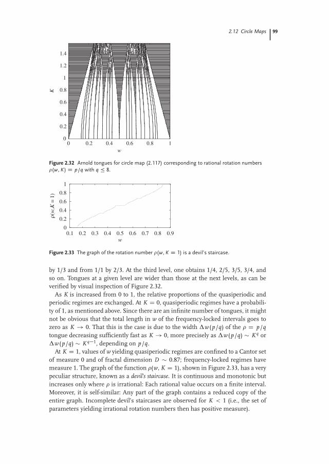
2.12 Circle Maps 99
0
0.2
0.4
0.6
0.8
1
1.2
1.4
0 0.2 0.4 0.6 0.8 1
K
w
Figure 2.32 Arnold tongues for circle map (2.117) corresponding to rational rotation numbers
�(w, K) D p/q with q � 8.
0
0.2
0.4
0.6
0.8
1
0.1 0.2 0.3 0.4 0.5 0.6 0.7 0.8 0.9
ρ(w
,K =
1)
w
Figure 2.33 The graph of the rotation number �(w, K D 1) is a devil’s staircase.
by 1/3 and from 1/1 by 2/3. At the third level, one obtains 1/4, 2/5, 3/5, 3/4, andso on. Tongues at a given level are wider than those at the next levels, as can beverified by visual inspection of Figure 2.32.
As K is increased from 0 to 1, the relative proportions of the quasiperiodic andperiodic regimes are exchanged. At K D 0, quasiperiodic regimes have a probabili-ty of 1, as mentioned above. Since there are an infinite number of tongues, it mightnot be obvious that the total length in w of the frequency-locked intervals goes tozero as K ! 0. That this is the case is due to the width Δw (p/q) of the � D p/qtongue decreasing sufficiently fast as K ! 0, more precisely as Δw (p/q) � K q orΔw (p/q) � K q�1, depending on p/q.
At K D 1, values of w yielding quasiperiodic regimes are confined to a Cantor setof measure 0 and of fractal dimension D � 0.87; frequency-locked regimes havemeasure 1. The graph of the function �(w, K D 1), shown in Figure 2.33, has a verypeculiar structure, known as a devil’s staircase. It is continuous and monotonic butincreases only where � is irrational: Each rational value occurs on a finite interval.Moreover, it is self-similar: Any part of the graph contains a reduced copy of theentire graph. Incomplete devil’s staircases are observed for K < 1 (i.e., the set ofparameters yielding irrational rotation numbers then has positive measure).
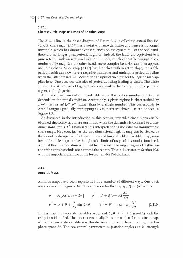
100 2 Discrete Dynamical Systems: Maps
2.12.3
Chaotic Circle Maps as Limits of Annulus Maps
The K D 1 line in the phase diagram of Figure 2.32 is called the critical line. Be-yond it, circle map (2.117) has a point with zero derivative and hence is no longerinvertible, which has dramatic consequences on the dynamics. On the one hand,there are no longer quasiperiodic regimes. Indeed, the latter are equivalent to apure rotation with an irrational rotation number, which cannot be conjugate to anoninvertible map. On the other hand, more complex behavior can then appear,including chaos. Since map (2.117) has branches with negative slope, the stableperiodic orbit can now have a negative multiplier and undergo a period doublingwhen the latter crosses �1. Most of the analysis carried out for the logistic map ap-plies here: One observes cascades of period doubling leading to chaos. The whitezones in the K > 1 part of Figure 2.32 correspond to chaotic regimes or to periodicregimes of high period.
Another consequence of noninvertibility is that the rotation number (2.118) nowdepends on the initial condition. Accordingly, a given regime is characterized bya rotation interval [��, �C] rather than by a single number. This corresponds toArnold tongues gradually overlapping as K is increased above 1, as can be seen inFigure 2.32.
As discussed in the introduction to this section, invertible circle maps can beobtained rigorously as a first-return map when the dynamics is confined to a two-dimensional torus T 2. Obviously, this interpretation is not valid for noninvertiblecircle maps. However, just as the one-dimensional logistic map can be viewed asthe infinitely dissipative of a two-dimensional horseshoelike invertible map, non-invertible circle maps can be thought of as limits of maps of an annulus into itself.Not that this interpretation is limited to circle maps having a degree of 1 (the im-age of the annulus winds once around the center). This is illustrated in Section 10.8with the important example of the forced van der Pol oscillator.
2.13
Annulus Maps
Annulus maps have been represented in a number of different ways. One suchmap is shown in Figure 2.34. The expression for the map (�, θ ) ! (�00, θ 00) is
�0 D �0�cos(πθ ) C 2θ
��00 D �0 C d (� � �0)
dθ 0
dθ
θ 0 D ω C θ C K2π
sin (2πθ ) θ 00 D θ 0 � d (� � �0)d�0
dθ(2.119)
In this map the two state variables are � and θ , 0 � θ � 1 (mod 1) with theendpoints identified. The latter is essentially the same as that for the circle map,while the new state variable � is the distance of a point from the origin in thephase space R2. The two control parameters ω (rotation angle) and K (strength

2.13 Annulus Maps 101
-10 -8 -6 -4 -2 0 2 4 6 8 10x
-6
-4
-2
0
2
4
6y
Figure 2.34 The transformation (�, θ ) ! (�00 , θ 00) invertibly maps the annular set (circles with
radii �˙ D �0 ˙ Δ� D 3.5, 6.5) onto the deformed set, shown with darker lines inside the
annulus. Parameter values: (�0, ω, K/2π, d) D (5.0, 0.0, 2.0, 0.06).
of nonlinearity) have the same meaning as for the circle map. The new controlparameter d is a measure of the dissipation: as d ! 0 we recover the circle map.
Annulus maps exhibit a variety of exciting behaviors. Some of this behavior isdescribed by the Afraimovich–Shilnikov torus breakdown theorem [85, 86]. Thistheorem is local in nature, describing a spectrum of behaviors in the neighborhoodof an Arnold tongue [83]. Annulus maps can support multiple coexisting basins ofattraction. This is made manifest by the occurrence of hysteresis in bifurcationdiagrams under some conditions. This type of global behavior is not covered by theAfraimovich–Shilnikov theorem.
We describe the Afraimovich–Shilnikov theorem as it applies to a period-3Arnold tongue in an annulus map. The tongue in a two-control parameter planeis indicated in Figure 2.35. The Arnold tongue is bounded by two saddle–nodebifurcation curves, labeled SNB1 and SNB2. Crossing these curves involves a di-rect or an inverse saddle–node bifurcation. For the period-3 tongue, this involvesthe creation or annihilation of a period-3 pair of orbits, one saddle and one node.“Opposite” the vertex of the Arnold tongue is a curve indicating the beginning ofa period-doubling cascade to chaos. The larger the period q of the p/q tongue, thefaster the transition through this region to chaos. Curves H o�
1 and H o�2 indicate
where there is a homoclinic connection between the stable and unstable manifoldsof the period-3 saddle orbit. These curves connect the saddle–node curves with theperiod-doubling curve. Outside the tongue curves H e1 and H e2 locate the hetero-clinic connection, the curve in control parameter space along which the unstablemanifold of the saddle is tangent to the stable manifold of the node. Below thisexterior region the behavior is quasiperiodic; above it is chaotic.
We now illustrate this behavior with the study by Letellier, Messager, andGilmore [87] of the dynamics of an annulus map introduced by Curry andYorke [88]. The Curry–Yorke map is defined as follows. Let Ψ1 and Ψ2 be two

102 2 Discrete Dynamical Systems: Maps
Figure 2.35 Schematic of an Arnold tongue
in a control parameter plane and the kinds
of behavior in its vicinity. SNB1, SNB2 are
saddle–node bifurcation curves. P D is
the first period-doubling bifurcation curve.
H o�1 , H o�
2 are curves indicating homo-
clinic connections, tangencies of the stable,
and unstable manifolds of the saddle cycle.
H e1, H e2 are curves defining the heteroclinic
connections of the unstable and stable man-
ifolds of the saddle and node period-3 orbits.
Path 1: Figure 2.36a–c. Path 2: Figure 2.36d–f.
homeomorphisms of the plane. Ψ1 is defined in polar coordinates (�, θ ) by
Ψ1(�, θ ) D �� ln(1 C �), θ C θ0
�(2.120)
and Ψ2 is defined in cartesian coordinates by
Ψ2(x , y ) D �x , x2 C y
�(2.121)
The Curry–Yorke map Ψ is obtained by composing these two maps: Ψ D Ψ2 ıΨ1.A complicated dynamics, typical of an annulus map, can be observed when thismap is iterated.
In the left part of Figure 2.36 we show snapshots of the attractor at three pointsalong Path 1 in Figure 2.35. In Figure 2.36a the motion is quasiperiodic on thetorus, which has been deformed to triangular shape in anticipation of the impend-ing saddle–node bifurcation that creates the stable period-3 node. The circles showthe location of the real part of the saddle node pairs just before the bifurcation.After the bifurcation there is a stable period-3 orbit. It is not shown here, but thelocations of the three points in this orbit are clear from the positions of their analyt-ic continuations in Figure 2.36a (just before entering the tongue) and Figure 2.36b(just after leaving the tongue). The torus is wrinkled (see insets, Figure 2.36b) onleaving the tongue above the curve H e1. There is a “hard” transition to chaos. Asthe control parameter moves further away from the boundary of the tongue, theattractor becomes increasingly wrinkled, as shown in Figure 2.36c.
Path 2 enters the tongue by crossing the other saddle–node boundary curveSNB2 below the heteroclinic curve H e2. Before entering the tongue the behav-ior is quasiperiodic. Once again the torus becomes deformed to a triangular shape

2.13 Annulus Maps 103
3
2
1yn
32.52
1.51
0.50
–0.5–1
–1.5
yn
0
0.2
–0.2
0.4
–0.4
–0.6
yn
2
3
1
4
5
0
–1
4
2
6
8
0
–2
yn
yn
xn
0
–1
3
2
1yn
0
–1
–2xn
–0.4 –0.2 0 0.2 0.4
xn–2 –1 0 1
xn–3 –2 –1 0 1 2
–1.5 –1 –0.5 0 0.5 1 1.5
xn–2 –1.5 –1 –0.5 0 0.5 1 1.5
xn–2 –1.5 –1 –0.5 0 0.5 1 1.5
(a)
(b)
(c)
(d)
(e)
(f)
Figure 2.36 (a–c) Snapshots of the attractor
at three points along Path 1 of Figure 2.35;
(a) quasiperiodicity is evident just outside the
left-hand boundary of the period-3 tongue and
below the heteroclinic curve H e1; (b) toroidal
chaotic behavior is exhibited after crossing
the tongue boundary above H e1. Wrinkling is
evident close to the remnants of the period-3
orbit (see insets): the real parts of the coor-
dinates are shown here; (c) toroidal chaos
becomes increasingly evident and the folding
more pronounced as the path receeds from
the tongue boundary; (d–f) snapshots of the
attractor at three points along Path 2 of Fig-
ure 2.35; (a) quasiperiodicity is evident just
outside the right-hand boundary of the period-
3 tongue and below the heteroclinic curve
H e2; (b) a banded period-3 chaotic attrac-
tor occurs after passage through the period-
doubling cascade and beyond the inverse
noisy period-halving bifurcations; (c) toroidal
chaos occurs after one or more crises increase
the size of the attractor. After Letellier, Mes-
sager, and Gilmore [87].
in anticipation of the impending saddle–node bifurcation. The dots shown in Fig-ure 2.36d indicate the locations of the real part of the period-3 orbit. The path exitsthe tongue through the period-doubling region. After the accumulation curve is

104 2 Discrete Dynamical Systems: Maps
crossed, a series of noisy period-halving bifurcations ensues, creating a banded(three bands) chaotic attractor. This is shown in Figure 2.36e. The locations of theperiod-3 orbit, stable inside the tongue but now unstable, are shown as dots. Afterone or more crises have taken place, a chaotic toroidal attractor is formed. This isshown in Figure 2.36f.
2.14
Summary
Although maps are very simple dynamical systems, they display most of the keyfeatures of chaos. This has allowed us to become familiar with concepts that willappear throughout this book, without excessive mathematical complexity.
Even the simplest dynamical system that one can think of, the logistic map, isable to reproduce surprisingly well qualitative behaviors that are observed exper-imentally in the laser system described in Chapter 1. As a control parameter isvaried, it experiences bifurcations, in particular a period-doubling cascade leadingto chaos, and a variety of chaotic regimes.
The simple structure of the logistic map makes it possible to study one of thebasic mechanisms responsible for chaotic behavior, namely stretching. In its mostchaotic regime, the logistic map is basically a “multiply by two” machine. This hasfar-reaching consequences: sensitivity to initial conditions, existence of an infinitenumber of periodic orbits that are dense in the invariant set, and so on.
Stretching is at the root of an extremely powerful tool for unfolding chaos, sym-bolic dynamics. Thanks to the unlimited magnification provided by sensitivity toinitial conditions, a series of coarse-grained measurements of the system state suf-fices to specify it with arbitrary accuracy. Symbolic dynamics not only allows us toclassify orbits (e.g., how many periodic orbits of period p?) but also to study theirgenealogies (e.g.: In what order do orbits appear? Which orbit is a period-doubledorbit from another?). By studying the grammar of a chaotic system, we can classifyregimes and compute quantitative invariants such as topological entropy. Not allof the results obtained (e.g., the universal sequence) can be directly extended tohigher dimensions. That there are topological invariants (e.g., permutations) bothof which are deeply related to symbolic dynamics and play a major role in forcingrelations will later prove to be a key property.
The logistic map is a noninvertible system. Many physical systems are describedby ODEs and thus are associated with invertible maps, such as the Hénon map. Achaotic invertible map shares many properties with noninvertible ones. In particu-lar, the dynamics in the unstable space is associated with a noninvertible map, asthe example of the horseshoe map shows. There are also new problems, such asconstructing relevant symbolic encodings in that case. Finally, global phase spacetopology can have a profound influence on phenomena observed, as exemplifiedby circle and annulus maps.