Introduction to DiscreteNonlinear Dynamical Systems

University of TrentoMarch 12-13, 2009

A. Agliari1, G-I Bischi2, L.Gardini2, I. Sushko3

1Dipartimento di Economia, Università di Piacenza, Italy.

2Dipartimento di Economia e Metodi Quantitativi,Università di Urbino, Italy.3Institute of Mathematics National Academy of Sciences ofUkraine, Kiev, Ukraine.

1

Contents

1 Definitions and preliminary notions. 4

2 One-dimensional phase-space. 82.1 Iterated Function System (IFS) . . . . . . . . . . . . . . 172.2 The chaos game and Random IFS . . . . . . . . . . . . . 19

3 Homoclinic theorem in 1D. 21

4 Dynamics in higher dimensional spaces. 244.1 Quadratic map. . . . . . . . . . . . . . . . . . . . . . . . 27

5 Homoclinic theorem for expanding periodic points. 32

6 Global Bifurcations of Invariant Sets and Homoclinic Tan-gles 386.1 Stable and unstable sets. Homoclinic tangle. . . . . . . . 386.2 Invariant closed curves . . . . . . . . . . . . . . . . . . . 436.3 Appearance of an invariant closed curve. A simple example 47

6.3.1 Saddle-node bifurcation for closed curves . . . . . 516.3.2 Saddle connections . . . . . . . . . . . . . . . . . 556.3.3 Saddle-node bifurcation of a cycle . . . . . . . . . 59

6.4 Interaction between invariant closed curves and cycles. Abusiness cycle model . . . . . . . . . . . . . . . . . . . . 616.4.1 From one repelling closed curve to two repelling

ones . . . . . . . . . . . . . . . . . . . . . . . . . 666.4.2 Interaction between coexisting invariant curve and

cycles. . . . . . . . . . . . . . . . . . . . . . . . . 71

7 Basin of attraction and related contact bifurcations. 787.1 One-dimensional maps . . . . . . . . . . . . . . . . . . . 787.2 Two-dimensional maps. . . . . . . . . . . . . . . . . . . . 81

7.2.1 Example 1: Quantity-setting duopoly gameswith adaptive expectations . . . . . . . . . . 82

7.2.2 Example 2: A rent-seeking/competition game . . 90

8 Piecewise smooth systems. 978.1 1D map. . . . . . . . . . . . . . . . . . . . . . . . . . . . 97

8.1.1 Chaotic intervals . . . . . . . . . . . . . . . . . . 1048.1.2 Border-collision bifurcation at G = 1 . . . . . . . 107

8.2 2D Business Cycle map. . . . . . . . . . . . . . . . . . . 1118.3 2D canonical form. . . . . . . . . . . . . . . . . . . . . . 120

8.3.1 Center bifurcation (δR = 1) . . . . . . . . . . . . 124

2

8.3.2 Bifurcation Diagrams in the (δR, τR)-parameter plane1298.3.3 1/n periodicity regions and their BCB boundaries 134

9 Appendix on the Myrber’s map. 140

10 Bibliography. 143

3

1 Definitions and preliminary notions.

The object of the present work is to describe some properties on thecomplex world of the nonlinear dynamics in discrete systems. Let usconsider a dynamic model which is described by iterating some process:

Fig.1 Iterative process

The state of the system changes under the action of some function, hererepresented (Fig.1) by T . The state x may be a scalar or a vector ofstate variables. The state (or phase) space is a set X ⊆ Rm wherem is an integer denoting the dimension of the vector state variable x,m ∈ 1, 2, 3... , and T : X → X. A discrete dynamical system (DDS forshort) is represented by the standard notation

xn+1 = T (xn) or x0 = T (x) (1)

The object of the theory of DDS is that to understand which kind ofvalues will be obtained asymptotically, and this depending on the initialvalue (or initial condition, i.c. henceforth) x0 in the phase space. Alsoimportant will be the bifurcations, which are responsible of the changesin the qualitative behaviors of the trajectories of the iterative process.To this scope we recall that the bifurcations are studied in the para-meter space, which includes all the parameters which are considered inthe model under study. Whenever the parameters have a fixed valuewe have a dynamic system whose invariant sets in the phase space ofinterest are our object of investigation, as well as the description of thedynamic behavior associated with the points in the phase space (are thetrajectories converging to the same set ? are some of them uninterestingfor us because associated to divergent dynamics ? and so on). Then,as the parameters are varied, things may change smoothly (as under adeformation, we shall say "via an homeomorphism", which is a contin-uous invertible function) or some drastic change may occur, in whichcase we say that a bifurcation takes place. Roughly speaking, we saythat a bifurcation takes place at some specific parameters setting whenthe dynamics occurring "before" and "after" (when the condition is notfulfilled) cannot be obtained one from the other by a smooth change (viaan homeomorphism).To study DDS it is important to introduce first a few definitions

and terms. Let us consider a map x0 = T (x), T is defined from X intoitself. The point x0 is called the rank-1 image of x. A point x such thatT (x) = x0 is called a rank-1 preimage of x0. The point x(n) = Tn(x),

4

n ∈ N, is called image of rank-n of the point x, where T 0 is identifiedwith the identity map and T n (·) = T Tn−1 (·) = T (T n−1 (·)). A pointx such that Tn(x) = y is called rank-n preimage of y.Let A ⊂ X be a such that T (A) ⊆ A, then A is called trapping

set. We have two kinds of trapping set: either (a) T (A) = A, then Ais called invariant set, or (b) T (A) ⊂ A than A is strictly mapped intoitself, and in this case T n+1(A) ⊆ T n(A) for any n > 0. When A isa compact set then the intersection of the nested sequence of sets is aclosed nonempty invariant set, say B = ∩n>0T n(A), then T (B) = B(note that the number of iterations necessary to get the invariant set Bmay be finite or infinite). For our purposes it is important to stress theproperties of an invariant set A ⊆ X. As by definition any point of T (A)is the image of at least one point of A, we have that for an invariant setA ⊆ X, for which T (A) = A, this propery holds for any point in A, thatis:Property 1. If T is invariant on A then any point of A has at least

one rank-1 preimage in A, and iteratively: any point of A has an infinitesequence of preimages in A.The behaviour of points in a neighburhood of an invariant set A

depends on the local dynamics (Amay be attracting, repelling, or neitherof the two).An attracting set is a closed invariant set A which possess a trapping

neighborhood, that is, a neighborhood U , with A ⊂ Int(U), such thatA = ∩n≥0T n(U) (as in the case of the set B constructed above). Inother words, if A is an attracting set for T , then a neighborhood U ofA exists such that the iterates Tn(x) tend to A for any x ∈ U (and notnecessarily enter A). An attractor is an attracting set with a dense orbit.The basin of attraction of an attracting set A, B(A), it the set of

all the points whose trajectory has the limit set in A (roughly speaking,whose trajectory tends to A).

B (A) = x|T n(x)→ A as n→ +∞ .As the attracting set possesses a neighborhood U of points having thisproperty, then the basin is made up of all the possible preimages of U :B(A) = ∪n≥0T−n(U). Sometimes it is useful to consider as neighborhoodU the immediate basin, which is the largest connected component of thebasin which contains the attracting set A.A repelling set is a compact invariant set K which possesses a neigh-

borhood U such that for any point x0 ∈ U\K, the trajectory x0 →x1 → ... must satisfy xn /∈ U for at least one value of n ≥ 0 (but such atrajectory may also come back again in U, as it occurrs when homoclinictrajectories exist). A repellor is a repelling set with a dense orbit.

5

It is worth noticing that this definition is a very strict one (as weshall see below, by using this definition a saddle cycle cannot be calledrepelling, but only unstable). Some authors use "expanding" in its place,keeping a more soft definition for a repelling set saying that a closedinvariant setK which is not attracting is called repelling if however closeto K there are points whose trajectories goes away from K. And as usuala repellor is defined as a repelling set containing a dense orbit. This lessrestrictive definition allows, when applied to a cycle, to say that attractor(repellor) is synonymous of asymptotically stable (unstable), however itis worth noticing that in this case we have further to distinguish whena repelling cycle is expanding or not.Regarding the invariant sets, the simplest case is that of "fixed point".

We say that x∗ is a fixed point (or equilibrium point) of the DDS if itsatisfies

x∗ = f(x∗)

That is: starting in that point the system never changes. Then, giventhat it is very difficult to be exactly in a fixed point, it is important tounderstand when (i.e. under which conditions) starting from a differentstate and iterating the process we are approaching the equilibrium, andwhen this occurs for all the points in a suitable neighborhood, we call itattracting: The definition given above is fulfilled. When for some points,also very close to an equilibrium, the process will lead the state far awayfrom it, then it is unstable.

Fig.2

A map T is said to be noninvertible (or “many-to-one”, see Fig.2), if dis-tinct points x 6= y exist which have the same image, T (x) = T (y) = x0.This can be equivalently stated by saying that points exist which haveseveral rank-1 preimages, i.e. the inverse relation x = T−1 (x0) may bemulti-valued. Geometrically, the action of a noninvertible map T can

6

be described by saying that it “folds and pleats” the plane, so that twodistinct points are mapped into the same point. Equivalently, we couldalso say that several inverses are defined, and these inverses “unfold”the plane. For a noninvertible map T , the space Rm can be subdividedinto regions Zk, k ≥ 0, whose points have k distinct rank-1 preimages(Fig.3). Generally, as the point x0 varies in Rm, pairs of preimages ap-pear or disappear as this point crosses the boundaries which separatedifferent regions. Hence, such boundaries are characterized by the pres-ence of at least two coincident (or merging) preimages. This leads to thedefinition of the critical sets, one of the distinguishing features of non-invertible maps (Mira et al., [89]): The critical set CS of a continuousmap T is defined as the locus of points having at least two coincidentrank − 1 preimages, located on a set CS−1 called set of merging preim-ages. The critical set CS is the n-dimensional generalization of thenotion of critical value (when it is a local minimum or maximum value)of a one-dimensional map1, and of the notion of critical curve LC of anoninvertible two-dimensional map (from the French “Ligne Critique”).The set CS−1 is the generalization of the notion of critical point (whenit is a local extremum point) of a one-dimensional map, and of the foldcurve LC−1 of a two-dimensional noninvertible map. The critical set CSis generally formed by (n− 1)-dimensional hypersurfaces ofRm, and por-tions of CS separate regions Zk of the phase space characterized by adifferent number of rank − 1 preimages, for example Zk and Zk+2 (thisis the standard occurrence).

Fig.3

1This terminology, and notation, originates from the notion of critical points asit is used in the classical works of Julia and Fatou.

7

2 One-dimensional phase-space.

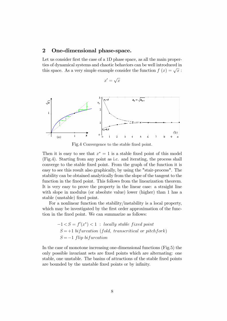
Let us consider first the case of a 1D phase space, as all the main proper-ties of dynamical systems and chaotic behaviors can be well introduced inthis space. As a very simple example consider the function f (x) =

√x :

x0 =√x

Fig.4 Convergence to the stable fixed point.

Then it is easy to see that x∗ = 1 is a stable fixed point of this model(Fig.4). Starting from any point as i.c. and iterating, the process shallconverge to the stable fixed point. From the graph of the function it iseasy to see this result also graphically, by using the "stair-process". Thestability can be obtained analytically from the slope of the tangent to thefunction in the fixed point. This follows from the linearization theorem.It is very easy to prove the property in the linear case: a straight linewith slope in modulus (or absolute value) lower (higher) than 1 has astable (unstable) fixed point.For a nonlinear function the stability/instability is a local property,

which may be investigated by the first order approximation of the func-tion in the fixed point. We can summarize as follows:

−1<S = f 0(x∗) < 1 : locally stable fixed point

S=+1 bifurcation (fold, transcritical or pitchfork)

S=−1 flip bifurcation

In the case of monotone increasing one-dimensional functions (Fig.5) theonly possible invariant sets are fixed points which are alternating: onestable, one unstable. The basins of attractions of the stable fixed pointsare bounded by the unstable fixed points or by infinity.

8

Fig.5 Increasing functions, piecewise linear and nonlinear smmoth.

In the linear case we can see that at the bifurcation occurring when theslope is equal to −1, a new kind of dynamics occurs: all the points be-long to a 2-cycle (Fig.6).

Fig.6 Decreasing linear functions

In the generic case of a decreasing one-dimensional function the onlypossible invariant sets are one fixed point, and 2-cycles, which are alter-nating: one stable, one unstable.We can already see a generic feature: if the slope in the fixed point is

positive (resp. negative) then locally we have monotonic dynamics (resp.alternating dynamics), as qualitatively shown in Fig.7a and Fig.7b, re-spectively.

9

Fig.7 Monotone dynamics or alternating dynamics.

Moreover we have seen that cycles may occur. A k−cycle is a sequence ofk distinc points xi, i = 1, 2, ..., k visited iteratively by the map, and suchthat fk(xi) = xi for any point xi. That is, stated in other words, each ofthe periodic points is a fixed point of the map fk = f f ... f. Thestability/instability of a cycle is determined by the stability/instabilitycondition of a fixed point of the map fk and from the chain rule we have,for each point xi of the cycle,

S =d

dx(fk(x))|xi =

kQj=1

f 0(xj) (2)

Summarizing, if we consider a one—dimensional map xn+1 = f(xn) anda k−cycle of points x1, ..., xk , k ≥ 1 (for k = 1 we have a fixed point),the condition |S| < 1 (resp. > 1) is a sufficient condition to concludethat the k−cycle is an attractor (resp. repellor), as S is the slope, oreigenvalue, in any point xi of the map fk.We have not considered the bifurcation cases in which |S| = 1, be-

cause the behavior depends on the kind of bifurcation. This can be foundin several textbooks ([104], [49], [50], [30], [70]), and we simply recall thatthe bifurcations associated with S = −1 are related to a period-doublingof the cycle, and it is frequently called flip bifurcation. That is, crossingthis bifurcation value, when suitable transversality conditions are sat-isfied, then a stable k−cycle becomes unstable and a stable 2k−cycle(of double period) appears around it. While the bifurcations associatedwith S = +1 may be of three different kinds: (i) either related to afold bifurcation, giving rise to a pair of k−cycles, one attracting andone repelling, (ii) or to a change of stability (also called transcritical),a pair of stable/unstable cycles merge after which they exchange theirstability, i.e. become unstable/stable respectively, (iii) or a pitchfork

10

bifurcation occurs at which a stable k−cycle becomes unstable and twonew k−cycles appear around it, both stable.As observed several years ago by the pioneers of such studies ([92],

[103], [85], [86], [82], [87]) still in the one-dimensional case we can seethat once that the monotonicity (i.e. the invertibility property) is lost,then very complicated paths may occur, which may be predictable or not(although the model is completely deterministic). As a standard examplelet us consider the simple logistic map (whose graph is a parabola):

x0 = f(x) , f(x) = µx(1− x) , µ ∈ [3, 4] (3)

which for µ > 3 has the origin as unstable fixed point and the pos-itive fixed point which may be stable or unstable, depending on theslope (or eigenvalue) in that point. This map has a unique critical pointc = µ/4, which separates the real line into the two subsets (see Fig.8):Z0 = (c,+∞), where no inverses are defined, and Z2 = (−∞, c), whosepoints have two rank-1 preimages. These preimages can be computedby the two inverses

Fig.8 Logistic map

x1 = f−11 (x0) =

1

2−pµ (µ− 4x0)2µ

; x2 = f−12 (x0) =

1

2+

pµ (µ− 4x0)2µ

.

(4)If x0 ∈ Z2, its two rank-1 preimages, computed according to (4), arelocated symmetrically with respect to the point c−1 = 1/2 = f−11 (µ/4) =f−12 (µ/4). Hence, c−1 is the point where the two merging preimages ofc are located. The map f folds the real line, the two inverses unfold it(Fig. 1b). As the map (3) is differentiable, at c−1 the first derivativevanishes. However, note that in general a critical point may even be apoint where the map is not differentiable. This happens for continuouspiecewise differentiable maps such as the well known tent map or otherpiecewise linear maps. In these maps critical points are located at the

11

kinks where two branches with slopes of opposite sign join and localmaxima and minima are located.As an equivalent model, we may consider any function which is ob-

tained by using a change of variable with an homeomorphism h (a con-tinuous and invertible function). We are so introducing the concept of"topological conjugacy": let

F = h f h−1 (5)

then the maps F and f are called topologically conjugated, and it canbe proved that topologically conjugated maps have the same dynamics:all the trajectories can be put in one-to-one correspondence by using thehomeomorphism h.It is easy to see that via a linear homeomorphism we can transform

the logistic map into the Myrber’s map (Myrber was the first author whostudied in details the bifurcations of such non-invertible one-dimensionalmaps, still in 1963):

x0 = F (x) : F (x) = x2 − b (6)

For b ∈ [0, 2] we have F : I → I, I = [q∗−1, q∗] where q∗ is the repelling

positive fixed point. At b = 0 the slope at the stable fixed point p∗ is zero(also called superstable), and then, increasing b, the slope from positivebecomes negative, reaching the value −1 and a flip bifurcation takesplace, leading to the appearance of a stable cycle of period 2 (Fig.9).

Fig.9 Attracting 2-cycle

From the shape of the second iterate of the function (Fig.10) we cansee that locally the fixed point of the map F 2 (2−cycle of F ) behavesas previously for the fixed point of the function F : the stable 2−cyclebecomes superstable. After that, the slope becomes negative, reachingthe value −1, and so on. By self-similarity all the cycles of period 2nwill be generated and become unstable leading, as n tends to infinity, to

12

a critical bifurcation value b = b∞2 after which the map has a so-calledchaotic behavior, because a set Λ invariant for the map, i.e. F (Λ) = Λ,on which the restriction is chaotic always exists.

Fig.10 Superstable 2-cycle

This is often represented in a bifurcation diagram (Fig.11) which showsthe asymptotic behavior of a generic point of the interval I = [q∗−1, q

∗]as a function of the parameter b.

Fig.11 Bifurcation diagram

The bifurcation diagram is "self-similar" as for any period (and severalboxes exist having the same period) we can repeat the period-doublingroute to chaos described above. As an example the enlargement showsthe "box" associated with the period-3 cycle: a pair of these cyclesappear by saddle node-bifurcation (see Fig.12a), and the stable one, forthe map F 3, will have the same bifurcation structure.

13

Fig.12 Box of the 3-cycle

We also note that although in a chaotic regime the dynamic behavioris unpredictable, some global properties can still be very useful. Forexample the iterates of the critical point determine cyclical intervalsor one single interval inside which the trajectories are confined, andsuch intervals are trapping: starting in a different point of the intervalI = [q∗−1, q

∗] a trajectory enters such absorbing interval from which itwill never escape (Fig.13).

Fig.13 Absorbing intervals

A "final bifurcation" is known to occur at the bifurcation value b = 2,when the preimage of the unstable fixed point becomes equal to thecritical value, that is: the invariant interval I = [q∗−1, q

∗] becomes aninvariant chaotic interval (Fig.14a), and after, for b > 2, the generictrajectory will be divergent. However a set which is invariant inside Iexists also for b > 2. As we shall see, it is a Cantor set on which therestriction of the map F is chaotic. Notice that in two iterations all the

14

points of the segment in the middle in Fig.14b are mapped above theunstable fixed point q∗, and then will diverge to +∞. The two distinctpreimages of this middle part will give two more intervals, one insideI0 and one inside I1, whose points are mapped, let us say "outside" q∗,in three iterations, and we continue this proces. Leaving from the oldinterval all the points whose trajectory will be divergent we are left withan invariant set Λ which is a Cantor set.

Fig.14 Full chaos in (a) and chaos in a Cantor set in (b).

A set Λ is a Cantor set if it is closed, totally disconnected and perfect2.The simplest example is the "Middle-third Cantor set": start with aclosed interval I and remove the open "middle third" of the interval(see Fig.15). Next, from each of the two remaining closed intervals, sayI0 and I1, remove again the open "middle thirds", and so on. After niterations, we have 2n closed intervals inside the two intervals I0 and I1.

Fig.15 Middle-third Cantor set

It is quite clear the similarity of this construction with that of the invari-ant set for the Myrberg’s map for any b > 2. Considering our unimodal

2Totally disconnected means that it contains no intervals (i.e. nosubset [a, b] with a 6= b) and perfect means that every point is a limitpoint of other points of the set.

15

map, for any point ξ belonging to the interval I = [q∗−1, q∗] there are two

distinct inverse functions, say F−1(ξ) = F−10 (ξ) ∪ F−11 (ξ), where

F−10 (ξ) = −pb+ ξ , F−11 (ξ) = +

pb+ ξ (7)

The set of points whose dynamics is bounded forever in the interval Ican be obtained removing from the interval all the points which exit theinterval after n iterations, for n = 1, 2, ..... Thus let us start with thetwo closed disjoint intervals

F−1(I) = F−10 (I) ∪ F−11 (I) = I0 ∪ I1, (8)

(see (Fig.14ab), i.e. we have removed the points leaving I after one iter-ation. Next we remove the points exiting after two iterations obtainingfour closed disjoint intervals

F−2(I) = I00 ∪ I01 ∪ I10 ∪ I11,defining in a natural way F−1(I0) = F−10 (I0) ∪ F−11 (I0) = I00 ∪ I10 andF−1(I1) = F−10 (I1) ∪ F−11 (I1) = I01 ∪ I11. Note that if a point x belongsto I01 (or to I11) then F (x) belongs to I1 (i.e. one iteration means drop-ping the first symbol of the index). Continuing the elimination processwe have that F−n(I) consists of 2n disjoint closed intervals (satisfyingF −(n+1)(I) ⊂ F−n(I)), and in the limit we get

Λ = ∩∞n=0F−n(I) = limn→∞

F−n(I). (9)

The set Λ is closed (as intersection of closed intervals), invariant byconstruction (as F−1(Λ) = F−1(∩∞n=0F−n(I)) = ∩∞n=0F−n(I) = Λ). Letus consider b > 2 and such that |F 0(x)| > 1 for any x ∈ I0 ∪ I1 (theproperty holds for any b > 2, but the proof is more complicated, it canbe found in [30]), then Λ cannot include any interval (because otherwise,since F is expanding, after finitely many application of F to an interval,we ought to cover the whole set I0∪ I1). Thus Λ is totally disconnected,and perfect by construction, so that it is a Cantor set.Moreover, by construction, to any element x ∈ Λ we can associate

a symbolic sequence, called Itinerary, or address, of x in the backwarddynamics, Sx = (s0s1s2s3...) with si ∈ 0, 1, i.e. Sx belongs to the setof all one-sided infinite sequences of two symbols Σ2. Sx comes from thesymbols we put as indices to the intervals in the construction process,and there exists a one-to-one correspondence between the points x ∈ Λand the elements Sx ∈ Σ2. Also, from the construction process we havethat if x belongs to the interval Is0s1...sn then F (x) belongs to Is1...sn.Thus the action of the function F on the points of Λ corresponds to the

16

application of the "shift map σ" to the itinerary Sx in the code spaceΣ2:

if x∈Λ has Sx = (s0s1s2s3...) (10)

then

F (x)∈Λ has SF (x) = (s1s2s3...) = σ(s0s1s2s3...) = σ(Sx)

Given a point x ∈ Λ how do we construct its itinerary Sx? In the obviousway: we put s0 = 0 if x ∈ I0 or s0 = 1 if x ∈ I1, then we consider F (x)and we put s1 = 0 if F (x) ∈ I0 or s1 = 1 if F (x) ∈ I1, and so on. Itfollows that F is chaotic in Λ, because it is topologically conjugated withthe shift map, which is the prototype of the chaotic map. We recall that,following the definition of chaos given by Devaney [30], an invariant setis chaotic under the action of a map F if

1) there exist infinitely many periodic orbits, dense in the invariant set

2) there exist an aperiodic trajectory dense in the set

As a consequence of the above two conditions we have that the sensitivitywith respect to the initial conditions also exists (which often is added asa third condition).However, it is easy to see that the two properties hold. If fact from

the correspondence given above we have that each periodic sequence ofsymbols of period k represents a periodic orbit with k distinct points,and thus a so-called k−cycle. Since the elements of Σ2 can be put inone-to-one correspondence with the real numbers3, we have that theperiodic sequences are dense in the space, thus (1): the periodic orbitsare dense in Λ. Also there are infinitely many aperiodic sequences (i.e.trajectories) which are dense in Λ thus (2) also is satisfied, and we alsohave sensitivity with respect to the initial conditions.

2.1 Iterated Function System (IFS)The construction process previously used, with the two contraction func-tions in (7) leading to the Cantor set in (9), can be repeated with anynumber of contraction functions defined in a complete metric space D ofany dimension4, as it is well known since the pioneering work by Barnsley(see [17], [18]). Let us recall the definition of an IFS:Definition. An Iterated Function System (IFS) D;H1, ...Hm is a

collection of m mappings Hi of a compact metric space D into itself.

3We can think for example of the representation of the numbers inbinary form.

4or better (D, d) where d denotes the function distance

17

We can so defineW = H1∪ ...∪Hm. Denoting by si the contractivityfactor of Hi then the contractivity factor of W is s = max s1, ...sm,and for any point or set X ⊆ D we define

W (X) = H1(X) ∪ ... ∪Hm(X).

The main property of this definition is given in the following theorem:Theorem (Barnsley 1988 [18] p. 82). Let D;H1, ...Hm be an IFS.

If the Hi are contraction functions then there exists a "unique attractor"Λ such that Λ =W (Λ) and Λ = limn→∞Wn(X) for any non-empty setX ⊆ D.

The existence and uniqueness of the set Λ is guaranteed by the the-orem and it is also true that given any point or set X ⊆ D by applyingeach time one of the m functions Hi the sequence tends to the same setΛ.In the case previously described with the Myrberg’s map we have

D = I, H1 = F−10 , H2 = F−11 .In general, if the sets Di = Hi(D) i ∈ 1, ...,m are disjoint, we can

put the elements of Λ in one-to-one correspondence with the elements ofthe code space on m symbols Σm. The construction is the generalizationof the process described above for the two inverses of the Myrberg’sfunction. Let U0 = D and define

U1=W (U0) = H1(D) ∪ ... ∪Hm(D) = D1 ∪ ... ∪Dm ⊂ U0

U2=W (U1) =W 2(U0) = H1(U1) ∪ ... ∪Hm(U1) = D11 ∪ ... ∪Dmm ⊂ U1

...

Un=W (Un−1) =W n(U0) ⊂ Un−1

i.e. all the disjoint sets of U1 are identified with one symbol belongingto 1, ...,m , all the disjoint sets of U2 are identified with two symbolsbelonging to 1, ...,m (m2 in number) and so on, all the disjoint sets ofUn are identified with n symbols belonging to 1, ...,m (mn in number).And in the limit, as Λ = limn→∞ Un = limn→∞Wn(U0) = ∩∞n=0Wn(U0),each element x ∈ Λ is in one-to-one correspondence with the elementsSx ∈ Σm, where Sx = (s0s1s2s3...), si ∈ 1, ...,m .Moreover, for any element x ∈ Λ we can define a transformation (or

map) F on the elements of Λ by using the inverses of the functions Hi

(the so called shift transformation or shift dynamical system in Barsnley1988, p. 144):

if x ∈ Hi(D) then F (x) = H−1i (D)

so that we can also associate an induced dynamic to the points be-longing to Λ, and the rule described above holds for F, i.e. if x ∈

18

Λ has itinerary Sx = (s0s1s2s3...) then F (x) ∈ Λ has itinerary SF (x) =(s1s2s3...) = σ(s0s1s2s3...) = σ(Sx). Clearly, when the functions Hi aredistinct inverses of a unique function f then the induced dynamic systemis the same, as F = f .

2.2 The chaos game and Random IFSAs a second relevant example (besides the logistic map) let us consideranother well known IFS with three functions, the so-called chaos game.Choose three different points Ai, i = 1, 2, 3, in the plane, not lyingon a straight line. Let D be the closed set bounded by the trianglewith vertices given by the three points Ai, and consider the systemD;H1,H2, H3 where the Hi are linear contractions in D with centerAi and contractivity factor 0.5. Then choose an arbitrary initial statex0 in D. An orbit of the system is obtained by applying one of thethree maps Hi, after throwing a dice. More precisely, xn+1 = Hi(xn)with i = 1 after throwing 1 or 2, i = 2 after throwing 3 or 4, i = 3after throwing 5 or 6. For any initial state x0 ∈ D, plotting the pointsof this orbit after a short transient gives Fig.16a. This fractal shape iscalled the Sierpinski triangle and it is the unique attractor of the chaosgame. Almost all the orbits generated in the chaos game are dense inthe Sierpinski triangle

Fig.16 (a) Sierpinski triangle, unique attractor Λ of the ITFD;H1, H2, H3 . (b) A subset Λ∗ of the Sierpinski triangle is the uniqueattractor of the RIFS D;H1, H2, H3 with the restriction that H1 is never

applied twice consecutively.

Moreover, in Barnsley (1988, p. 335) it is also shown how, besides thestandard IFS, we can consider a Random IFS (RIFS for short, or IFSwith probabilities) by associating a probability pi > 0 to each functionHi, such that Σm

i=1pi = 1. Considering a point x0 ∈ D then we chooserecursively

xn+1 ∈ H1(xn), ..., Hm(xn)

19

and the probability of the event xn+1 = Hi(xn) is pi. The iterated pointsalways converge to the unique attractor Λ of the standard IFS, but thedensity of the points over the set Λ reflects in some way the chosenprobabilities pi. However, we note that if the probabilities in the RIFSare strictly positive, pi > 0, then the unique attractor does not change,and the iterated points are dense in Λ.This may be very useful and convenient when using IFS theory ap-

plied to backward dynamic models. Using an approach similar to theRandom IFS, we can define a Restricted IFS (or IFS with restrictions)imposing that, depending on the position of a point x ∈ D not all themaps Hi can be applied but only some of them. Stated differently, wecan impose some restrictions on the order in which the functions canbe applied. As an example let us consider the chaos game describedabove, but now with some restrictions, that is: The order in which thethree different maps Hi are applied is not completely random, but sub-ject to certain restrictions. Suppose for example that the map H1 isnever applied twice consecutively, i.e. whenever H1 is applied then thenext map to be applied is either H2 or H3. Let Σ3 be the code space onthree symbols, and let Σ∗ ⊂ Σ3 be the subset of all sequences which donot have two consecutive 1’s. The chaos game D;H1,H2, H3 with therestriction so described has a unique attractor Λ∗ whose points are inone-to-one correspondence with the restricted space Σ∗. A typical orbitof this chaos game with restrictions, after a short transient, is shownin Fig.16b. The unique attractor of the chaos game with restrictionsis a subset of the Sierpinski triangle, the attractor of the chaos game.In fact, the attractor contains precisely those points of the Sierpinskitriangle whose itinerary, or addresses, do not have two consecutive 1’s.This example shows that when some restrictions upon the order in

which the maps are applied is imposed, then a unique fractal attractorcan arise, which is some subset of the unique attractor of the IFS.In the following sections we shall see how IFS are related in a nat-

ural way to non-uniquely defined forward sequences within a backwardmodel. We will also see that the forward states can be described by IFS,whenever the uniquely defined dynamics has homoclinic trajectories dueto the existence of a snap-back repellor.In the next section we shall show applications of the above theorem

associated with the existence of homoclinic orbits.

20

3 Homoclinic theorem in 1D.

Note that the main property in the previous construction is the existenceof two disjoint intervals, I0 and I1, such that

F k(I0) ⊃ I0 ∪ I1 and F k(I1) ⊃ I0 ∪ I1for a suitable k, and indeed this propery is the key feature in any dimen-sion, i.e. to prove the existence of chaos for maps in Rn whith n ≥ 1.We shall recall this in general in Section 5, but let us here briefly recallits application to the one-dimensional case, where a similar property(leading to the construction of an invariant set on which the restrictionof the map is chaotic) can be repeated whenever we have a homoclinictrajectory to some fixed point or cycle. A homoclinic trajectory to acycle is one which tends to the cycle in the forward process, and in somebackward one. For example, in a unimodal map it is easy to see whenthe unstable fixed point p∗ becomes homoclinic (also called snap backrepeller, after Marotto [79]). See also Fig.17 where in a neighborhood Uof p∗ we can find two intervals I0 and I1 such that fk(I0) ⊃ I0 ∪ I1 andfk(I1) ⊃ I0 ∪ I1 for a suitable k.

Fig.17 Homoclinic trajectory

In general we can state the following property for a unimodal map witha local maximum (and a similar property with obvious changes holds fora unimodal map with a local minimum):Let xm be the maximum point of a unimodal continuous map of an

interval into itself, say f : I → I, smooth in I\ xm , with a uniqueunstable fixed point x∗, and a sequence of preimages of xm tends to x∗.Then the first homoclinic orbits (all critical) of the fixed point x∗ occurwhen the critical point satisfies f3(xm) = x∗. For f3(xm) < x∗ the

21

fixed point is a snap-back repellor. There exists a closed invariant setΛ ⊆ [f2(xm), f(xm)] ⊆ I on which the map is topologically conjugate tothe shift automorphism, and thus f is chaotic, in the sense of Devaney(i.e. topological chaos, with positive topological entropy).

The proof of the bifurcation condition is immediate, as for f3(xm) >x∗ the fixed point x∗ has no rank-1 preimages in I, while at f3(xm) = x∗

the critical point is homoclinic and infinitely many homoclinic trajecto-ries exist, all critical. When f3(xm) < x∗ then infinitely many noncriticalhomoclinic orbits exist (close to those critical at the bifurcation value,that is, the homoclinic points are obtained by the same sequences ofpreimages of the function). So that the fixed point x∗ becomes a snap-back repellor.Then the existence of chaotic dymanics associated with noncritical

homoclinic orbits, let us call it "homoclinc theorem", is well known in aone-dimensional space (see for example [79], [30], [40]). In Section 5 weshall give a different proof of this "homoclinc theorem" for expandingcycles in any dimension n ≥ 1, by using the ITS.It is plain that the same result (that is, the existence of a closed

invariant set Λ on which the map is chaotic) holds for any cycle (pe-riodic point of any period), when it is a snap-back repellor (i.e. whenhomoclinic orbits exist), because the proposition above can be appliedto fixed points of the map fk, for any k > 1 (in suitable intervals for fk,corresponding to cyclical intervals for f).In Fig.11, showing the bifurcation diagram of the Myrberg’s map,

such invariant sets with chaotic dynamics occur for any b > b∞2 (whichrepresents the limit of the first period doubling sequence, after which thecycles of period 2n become homoclinic in decreasing order of period).

Fig.18

A remarkable application of this theorem in the economic context occursin the study of models formulated in the so called “backward dynam-ics”. That is, as discrete models in the form xt = F (xt+1), and the

22

interest is in the behavior of the forward values of the state variable(xt, xt+1, xt+2...). Two well known examples are the overlapping gener-ations (OLG)-model (e.g. Grandmont, 1985 [45], [46], [101], [47]) andthe cash-in-advance model (e.g. Woodford, 1994 [117], Michener andRavikumar, 1998 [84]). There are no problems when the function F (.)is invertible (as xt+1 = F−1(xt) is a standard dynamical system), whiledifficulties arise in the cases in which the function F (.) has not a uniqueinverse, and difficulties may also arise in the interpretation of the mod-els. Mathematically, this kind of models have been investigated consid-ering the space of all possible sequences, which is a space of infinitedimension (the so-called Hilbert Cube), and is known as Inverse LimitTheory (for the interested reader we refer to [60], [61] and the referencestherein). As applications to economic models see [83], [65], [66]. How-ever, the inverse limit approach is rather abstract (as it always considersinfinitely many states all together at once, without a real selection ofthe states step by step), so we prefer to follow a different approach,which is based on the theory of Iterated Function Systems. As statedabove, we show a kind of "bridge" between the theory of DynamicalSystems and the theory of IFS, which is useful to describe fractal "at-tractors" in the forward states of backward models. In [43] it is proposedthis technique applied to a one-dimensional model due to Grandmond,where the shape of the one-dimensional unimodal map fµ(.) is reportedin Fig.18a (whose bifurcation diagram is shown in Fig.18b). Anotherexample is in [83], where it is proposed an overlapping generation modelrepresented by the backward model with the one-dimensional logisticmap xt = fµ(xt+1) = µxt+1(1 − xt+1) already seen in Section 2, andtopologically conjugated with the Myrberg’s map.Let us consider the one-dimentional unimodal map fα(.) shown in

Fig.18a and let α∗ the bifurcation value at which the unstable fixedpoint becomes a snap-back repellor. Then for any α > α∗ there arenoncritical homoclinic orbits of x∗. Let us consider an example, andlet O(x∗) = x∗, x1, x2, ...xp, ... be the homoclinic orbit (an exampleis given in Fig.17) such that x1 = f−11 (x

∗) (while x∗ = f−10 (x∗)), and

xi = f−10 (xi−1) for any i > 1.Let U be a neighborhood of x∗ in which fµ(.) is expanding and such

that U1 = f−40 f−11 (U) ⊂ U, U0 = f−50 (U) (clearly U0 ∩ U1 = ∅).Then we have that G = f−50 (.) and F = f−40 f−11 (.) are contractionsin S = U0 ∪ U1. Thus S;F,G is an Iterated Function System ( IFS)which has a unique attractor Λ ⊂ S: an invariant Cantor set on whichfα is chaotic.To find some particular sequences in the forward process, for any

initial condition x0 ∈ S let us consider the following rule: whenever we

23

apply the left inverse f−11 then we apply the right inverse f−10 for atleast 4 times consecutively, i.e. any number q of times with the onlyrestriction q ≥ 4. It is clear that the sequence of forward states of thebackward model always belongs to the set A =

4Si=0

Si where S0 = S,

S1 = f−11 (S), Si = f−10 (Si−1) for i = 2, 3, 4, and the points have a kindof chaotic behavior in this set.The "rules" which we may construct leading to bounded forward

sequences (which seem chaotic) are infinitely many. Thus it depends onthe applied meaning of the model to have meaningful rules or not. In theeconomic context such rules may be associated to "sunspot" dynamics([25], [117], [13]).

4 Dynamics in higher dimensional spaces.

After the one-dimensional case let us consider m−dimensional dynam-ical systems T : X → X, X ⊂ Rm, m > 1. The definition of the localstability of a fixed point x∗ can be easily extended by using the lineariza-tion of the map, that is, the Jacobian matrix evaluated at the fixed pointJT (x

∗). When all the eigenvalues are less than 1 in absolute values thenthe fixed point is locally attracting, when one eigenvalue is higher than1 in absolute values then the fixed point is unstable.For real eigenvalues we have properties similar to those already de-

scribed in the one-dimensional case. That is, when one eigenvalue λcrosses through λ = −1 then a flip bifurcation may occur, while whenone eigenvalue λ crosses through λ = +1 then we may have a saddle-node or a transcritical or a pitchfork bifurcation. However now we haveone more kind of bifurcation, related with a pair of complex conjugatedeigenvalues which cross the modulus 1. This new kind of bifurcation isthe discrete analogue of the Hopf bifurcation for flows (dynamical sys-tems in continuous time), and it is called Neimark-Sacker (NS for short)bifurcation in the discrete case (associated with the names of the re-searchers who first and independently studied this kind of bifurcation).The existence of complex eigenvalues is also reflected in the dynamicbehaviors of the trajectories, which are oscillating around the equilib-rium, spiraling toward it when attracting or spiraling far from it whenunstable. The NS bifurcation is associated with the existence of closedinvariant curves around the fixed point or cycle (which, as usual, canbe studied as a fixed point for the iterated map). Let us recall here theNeimark-Sacker bifurcation theorem for a two-dimensional map ([50],[70]):

24

Fig.19

Let Fµ : R2 → R2 be a one-parameter family of 2D maps which has asmooth family of fixed points x∗(µ) at which the eigenvalues are complexconjugates λ(µ), λ(µ). Assume(1) |λ(µ0)| = 1, but λj(µ0) 6= 1 for j = 1, 4;(2) d

dµ(|λ(µ0)|) = d 6= 0. (transversality condition)

Then there is a smooth change of coordinates h so that the expressionhFµh

−1 in polar coordinates has the form hFµh−1(r, θ) = (r(1 + d(µ −

µ0) + ar2), θ + c+ br2)+ higher-order terms. If, in addition,(3) a 6= 0,then there is a 2D surface Σ (not necessarily infinitely differentiable)

in R2 ×R having quadratic tangency with the plane R2 × µ0 which isinvariant for Fµ. If Σ ∩ (R2 × µ0) is larger than a point, then it is asimple closed curve.The sign of the coefficients d and a determine the direction and sta-

bility of the bifurcating orbits, while c and b give information on the rota-tion numbers. The NS bifurcation is called supercritical (when a < 0) orsubcritical (when a > 0) (Fig.19). We remark that numerically one candeduce the type of the bifurcation just from the stability of the fixedpoint at the bifurcation value: If the fixed point is locally attracting(resp., repelling), then the NS bifurcation is supercritical (resp., subcrit-ical).A qualitative example is shown in Fig.20, where we can see that after

its appearance, via supercritical NS bifurcation, a closed invariant curveΓ may undergo several local and global bifurcations, leading to chaoticdynamics which often are related with an annular shape.

25

Fig.20

Let us notice that for 2D linear maps the condition a 6= 0 is obviouslynot satisfied, and not only at the fixed point, but in the whole regionof definition of the map. And, indeed, considering a linear map, say,Fµ, with complex-conjugate eigenvalues λ(µ), λ(µ), if |λ(µ0)| = 1 thenthe fixed point x = x∗(µ0) of Fµ is a center, so that the trajectory ofany point x 6= x∗(µ0) belongs to a related invariant ellipse and is eitherperiodic, or quasiperiodic, depending on the parameters. For µ 6= µ0the fixed point is either a globally attracting focus or a repelling focus(in which case the trajectory of any point x 6= x∗(µ) goes to infinity).Thus the bifurcation which occurs in a 2D linear map when its complex-conjugate eigenvalues cross the unit circle is called center bifurcation.In the particular case of a 2D map

T :

½x0 = F1(x, y)y0 = F2(x, y)

then the stability analysis at a fixed point X∗ = (x∗, y∗) is quite sim-ple. Let JT (X∗) be the jacobian matrix evaluated at the fixed point,of elements Jij , then we have to consider the eigenvalues, roots of thecharacteristic polynomial

P (λ) = det(JT (X∗)− λI) = λ2 − Trλ+Det = 0

whereTr = J11 + J22 , Det = J11J22 − J12J21

then the following conditions are necessary and sufficient to have all theeigenvalues less than 1 in modulus:

i) P (1)=1− Tr +Det > 0

ii) P (−1)=1 + Tr +Det > 0

iii) Det< 1

26

In the parameter plane (Tr,Det) the three conditions i), ii), iii) arethree straight lines which bound a triangle (known as stability triangle,see Fig.21), and when the parameters are such that the representativepoint (Tr,Det) is inside the triangle then the fixed point is locally at-tracting. The bifurcation occurring when P (1) = 0 is associated withone eigenvalues equal to +1, the one occurring when P (−1) = 0 is as-sociated with one eigenvalues equal to −1, while the NS bifurcation isassociated with the condition Det = 1 (the curve inside the triangleseparates real from complex eigenvalues).

Fig.21 Stability triangle

4.1 Quadratic map.In the case of maps in Rm, m > 1, chaotic dynamics may occur (as-sociated with homoclinic orbits) also in invertible maps (as a standardexample we may refer to the Henon map). While the true extension ofthe properties of the Myrberg map can be analyzed in a two-dimensionalnon-invertible map. As a prototype let us consider the map T definedby

T :

½x0 = ax+ yy0 = b+ x2

which was considered in [89] and [1]. The points which are the analogueof the critical points of a one-dimensional map are now associated withthe vanishing of the Jacobian determinant. Here we have

JT (x, y) =

·a 12x 0

¸, det JT (x, y) = −2x

then the set defined by detJT (x, y) = 0, here x = 0, represents theso called critical line LC−1 (from the french Ligne Critique, see in [51],

27

[52]), and its image, LC = T (LC−1) here the line of equation y = b,is a set which separates the phase plane into two regions: Z0 and Z2.Each point belonging to Z0 has no rank-1 preimage, while each pointbelonging to Z2 has two distinct rank-1 preimages, located one on theright and one on the left of LC−1.

Fog.22 Foliation of the plane

In a generic two-dimensional map, and in analogy of the one-dimensionalcase, the set LC−1 is included in the set where det JT (x, y) changes sign,since T is locally an orientation preserving map near points (x, y) suchthat det JT (x, y) > 0 and orientation reversing if det JT (x, y) < 0. Alsoin this case, when the map is continuously differentiable the points ofLC−1 necessarily belong to the set where the Jacobian determinant van-ishes, and LC = T (LC−1) belongs to boundaries which separate regionsZk characterized by a different number of preimages. In order to give ageometrical interpretation of the action of a multi-valued inverse relationT−1, it is useful to consider a region Zk as the superposition of k sheets,each associated with a different inverse. Such a representation is knownas Riemann foliation of the plane (see e.g. Mira et al., [89]). Differentsheets are connected by folds joining two sheets, and the projections ofsuch folds on the phase plane are arcs of LC. This is shown in the qual-itative sketch of Fig.22, where the case of a Z0 − Z2 noninvertible mapis considered. This graphical representation of the unfolding action ofthe inverses gives an intuitive idea of the mechanism which causes thecreation of non-connected basins for noninvertible maps of the plane.We can easily extend the definition given above to them-dimensional

case. It is clear that the relation CS = T (CS−1) holds, and the pointsof CS−1, in which the map is continuously differentiable, are necessarilypoints where the Jacobian determinant vanishes. In fact, in any neigh-borhood of a point of CS−1 there are at least two distinct points whichare mapped by T in the same point. Accordingly, the map is not locallyinvertible in points of CS−1.

28

Fig.23

As it occurs in one-dimensional maps, where absorbing intervals arebounded by the images of the critical point, also now the images ofthe critical curve (also called critical curves of higher rank) are used tobound absorbing areas as well as chaotic areas. An example of chaoticarea is shown in Fig.23, and in [89] it is proved that the boundary ofthe chaotic area is given by portions of critical curves belonging to theimages of the segment (called generating arc g) of LC−1 belonging tothe area itself.The white area in Fig.24 shows the basin of attraction of the chaotic

attractor, while gray points denote points having divergent trajectories.The basins also may have a fractal (or chaotic) structure, and a basinmay be simply connected, or connected but not simply or disconnected(which cannot occur in invertible maps), as we shall see in Section 7.The bifurcations leading to changes in the structure of the basins

(connected, multiply connected or disconnected) are called contact bi-furcations (see in [89]) because they are due to the contact of the fron-tier of the basin with the critical set LC. While bifurcations leading tochanges in the structure of the chaotic areas (reunion of chaotic pieces,explosion to a wide area, final bifurcation, etc.) are also called contactbifurcations but due to the contact of two (at least) different invariantsets.

29

Fig.24

It is clear now that things may be extended also to dynamics of a map Tin higher dimensions (m ≥ 3), although the related properties are morecomplicated for the analysis.As already recalled, the simplest analysis is that of the local stability

of equilibria. In particular we mention that when all the eigenvalues arein modulus higher than 1 then the fixed point (clearly unstable) is calledexpanding. Among the relevant notions associated with fixed pointsand k−cycles (fixed points of the map T k) we always have the notion ofhomoclinic trajectories, as these are the basic tools to rigorously show theexistence of chaotic dynamics. For expanding fixed points the extensionof the properties of the one-dimensional case is very simple, and relatedwith the properties of T k(I0) ⊃ I0∪I1 and T k(I1) ⊃ I0∪I1 for a suitablek, as we shall see in the next Section.However, homoclinic orbits may now also be related with saddle cy-

cles. For example, in a two-dimensional case, a saddle fixed point S orcycle C is characterized by a stable manifold, or more generally by astable set, denoted as W s(C) which is defined as the set of points whoseforward trajectory tends to C (and in 2D it is made up of two branchesω1 ∪ ω2), and by an unstable set, denoted asW u(C) which is defined asthe set of points for which at least a sequense of preimages exist leadingto C (and in 2D it is made up of two branches α1 ∪ α2) Then wheneverwe have W s(C)∩W u(C) 6= ∅ we have homoclinic points and chaotic sets

30

exist associated with a homoclinic orbit. A point q ∈ W s(C)∩W u(C) iscalled homoclinic to C as the sequence of its forward images tends toC and a suitable sequence of preimages also tends to C. The chaoticdynamics associated to such a homoclinic orbit is well known since theworks of Smale (Smale horseshoe) and the homoclinc tangle associatedto it, shown in Fig.25, will be described in Section 6.

Fig.25 Homoclinic tangle in a saddle fixed point S.

Before closing this section we recall that in higher dimensions the exis-tence of a closed invariant curve may occur not only via a NS bifurcation,as stated in Section 3, but also via global bifurcations connected withthe homoclinic tangles of saddle cycles, as we shall see in Section 6.

Fig.26

As an example, in Fig.26 we show several closed invariant curves, whoseexistence is not related with a NS bifurcation. In that example we havean attracting curve ΓS and two repelling curves eΓ1 and eΓ2.This case,occurring in a simple invertible map, may be found in [6].

31

5 Homoclinic theorem for expanding periodic points.

Here we recall how chaotic behaviors exist in a dynamical system when-ever we have transverse (which means non critical) homoclinic orbits ofexpanding cycles, also called snap-back repellors by Marotto. Withoutloss of generality we can deal with an expanding fixed point x∗ of a C(1)map T from a space X into itself, X ⊂ Rm with m = 1, as for a cycleof period k we can consider the map T k (k − th iterate of T ).We recall that a fixed point x∗ is hyperbolic if all the eigenvalues

of JT (x∗) are different from 1 in modulus, when all are higher then 1in modulus, then x∗ is expanding. Also, a homoclinic trajectory of afixed point x∗ is called non degenerate (or non critical, or transverse) ifdetJT (.) 6= 0 in all the points of the homoclinic trajectory.Definition. A fixed point x∗ of a smooth dynamical system is called a

snap-back repellor if it possesses a neighborhood U such that the Jacobianmatrix has all the eigenvalues higher than 1 in modulus in all the pointsof U, and in U there exist a homoclinic point of x∗.It is well known (as recalled before) that in any neighborhood of a

nondegenerate homoclinic trajectory we can find an invariant set Λ inwhich a suitable iterate of T , and thus T , is chaotic in the sense of Liand Yorke [71]. For the proof we refer to [30], [79], [80]. Here we give adifferent proof, showing its connection with the IFS ([40], [43], [115]).The proof consists in showing that in any neighborhood U of x∗ we

can find two disjoint compact sets, U0 and U1, U0 ∩ U1 = ∅, such thatfor a suitable k we have

T k(U0) ⊃ U0 ∪ U1 and T k(U1) ⊃ U0 ∪ U1 (11)

thus for the map T k there exists an invariant chaotic set Λ ⊂ U0 ∪ U1.In the following we illustrate:( I) how the set property in (11) is used to construct an invariant

Cantor set Λ ⊂ U0 ∪ U1, on which T k, and thus T , is chaotic;(II) how the set property in (11) can be found associated with a

given homoclinic trajectory;(III) an economic application.

Fig.27 Qualitative picture showing the application of F and G on the setsU0 and U1.

32

( I) We repeat here the process already used in Section 2 in the1D space. Let us consider eT = T k. As, from (11), eT (U0) ⊃ U0 then asuitable inverse, say F = eT−10 , exists such that F (eT (U0)) = U0, and aseT (U1) ⊃ U1 (from (11) as well) then a suitable inverse, say G = eT−11 ,

exists such that G(eT (U1)) = U1.Let S = U0∪U1 then F (S) is made up of two disjoint pieces U00 ⊂ U0

and U10 ⊂ U0, and the action of the map eT on such sets may be read onthe symbols which label the set, dropping the first symbol: eT (U00) = U0and eT (U10) = U0 (see the qualitative picture in Fig.27). Similarly G(S)is made up of two disjoint pieces U01 ⊂ U1 and U11 ⊂ U1, and the actionof the map eT on such sets may be read on the symbols which label theset, dropping the first symbol: eT (U01) = U1 and eT (U11) = U1. And soon, by repeating this mechanism we construct, in the limit process, aset Λ ⊂ S = U0 ∪ U1, Λ = ∩∞n=0(F ∪ G)n(S). The elements (or sets)Vs of Λ are in 1− 1 correspondence with the elements s = (s0s1s2s3...)(si ∈ 0, 1) of the space

P2 of (one sided) infinite sequences on two

symbols. Moreover the action of the map eT in Λ corresponds to theaction of the shift map σ to elements of Σ2, that is: if x is a point ofΛ and x ∈ Vs then eT (x) ∈ Vσ(s) (when s = (s0s1s2s3...) the shift mapdrops the first symbol σ(s) = (s1s2s3...) ).

Fig.28 Homoclinic trajectory in the phase plane, and neighborhoods I0 andI1.

This set Λ constructed up to now, without any other information on themap eT , is invariant (eT (Λ) = Λ), and its elements satisfy Vs 6= ∅ forany s, and Vs ∩ Vs0 = ∅ for s 6= s0 : It is what we call a set with Cantorlike structure, and its elements Vs are closed and compact (and thus Λis closed and compact) and simply connected if so are the starting setsU0 and U1.When F and G are "contraction mappings" then Λ is a classical

33

Cantor set of points. In fact, if the inverses F andG of eT are contractionsin U (or in S = U0 ∪ U1), the we can apply the IFS theory which statesthat U ;F,G is an Iterated Function System ( IFS) (or S;F,G is aIFS) which has a unique attractor Λ ⊂ U (or S): an invariant Cantorset on which the map eT is chaotic.(II) Now we show that the conditions in (11) are satisfied, and the

functions constructed in (II) are contractions, when we have a repellingfixed point (or cycle), unstable node or unstable focus, and a non degen-erate homoclinic trajectory, which means that the preimages of the fixedpoint belonging to the considered homoclinic orbit are not on the crit-ical curves (while degenerate homoclinic trajectories denote homoclinicexplosions). So that we prove the following:

Theorem. If a fixed point x∗ is expanding for a C(1) map T in X ⊆ Rm

with a non degenerate homoclinic orbit, then in any neighborhood of thehomoclinic orbit there exist an invariant set Λ on which T is chaotic.

Proof. Consider a compact neighborhood U of x∗ in which T isexpanding (i.e. all the eigenvalues of JT (x) are higher then 1 in modulusfor all the points x in U). Let us first show that under the assumptionsof the theorem we can always find two disjoint compact sets in U , U0 andU1, U0 ∩ U1 = ∅, such that for a suitable k we have T k(U0) ⊃ U0 ∪ U1and T k(U1) ⊃ U0 ∪ U1. Then we show that two suitable inverses arecontractions, so that the result comes from the properties descibed in(I).Let O(x∗) = x∗, x1, x2, ...xp, ... be the homoclinic orbit, and let

T−11 be the local inverse, satisfying T−11 (x∗) = x∗ and T−10 the inversesuch that T−10 (x∗) = x1, while the point xp is such that the repeatedapplications of T−11 to xp converge to x∗. Notice that T−10 (U) ∩ U = ∅.The nondegeneracy implies that DetJT (xi) 6= 0 in all the points of thehomoclinic orbit. The expansivity in a neighborhood implies that T−11is a contraction in U or locally homeomorphic to a contraction, but wecan choose a suitable integer p such that T−p1 is a contraction in U.Define G = T−p1 , and U1 = G(U). Then we apply to U the sequenceof inverses which follow the homoclinic orbit until we have again pointslocated inside U (see the qualitative picture in Fig.28). Define F =T−s1 ...T−11 T−10 where the integer s is such that F (U) ⊂ U and F is acontraction in U. Define U0 = F (U). Obviously x∗ ∈ U1, U1 and U0 aredisjoint (because T−11 (U) and T−10 (U) are disjoint by construction), andthus all the applications of the inverses by T−11 give disjoint sets, andby properly choosing the integers p and s (number of local inverses withT−11 ) in the construction of G and F we can assume k = p and such thatT k(U0) = U ⊃ U0 ∪ U1 and T k(U1) = U ⊃ U0 ∪ U1, so that U ;F,G isan Iterated Function System (IFS) which has a unique attractor Λ ⊂ U :

34

an invariant cantor set on which T k, and thus T , is chaotic, which endsthe proof.(III) An application of this theorem to a two dimensional model

in backword dynamics is described in [43] from an overlapping genera-tion model due to Grandmond [45], to which we refer for its deduction.Here let us briefly say that it refers to a map T of the plane into it-self of so-called Z0 − Z2 type: there exists a critical line LC−1 in whichDetJT (X) = 0 for any X ∈ LC−1, mapped into a line LC = T (LC−1)which separates the plane in to regions: Z0 whose points have no rank-1 preimages and Z2 whose points have two distinct rank-1 preimages,T−1R (.) and T

−1L (.) giving one point on the right and one point on the left

of LC−1, respectively. Explicitely, we have that the backward dynamicsis described by the two-dimensional backward map

(xt, yt) = T (xt+1, yt+1) = (f [a(1− δ +1

a)xt+1 − ayt+1], yt+1).

where the function f is unimodal, and its shape is reported in Fig.17and Fig.18. Thus we have the two inverses of T , associated with the twodistinct inverses of f , given by

T−1i :

½xt+1 = yt

yt+1 = (1− δ + 1a)yt − 1

af−1i (xt)

where i = L,R. At suitable values we have the fixed point X∗ of thefunction T, at the L side with respect to LC−1, which is an unstable fo-cus, with homoclinic points, i.e. it becomes a snap-back repellor. Thenwe may consider backword dynamics as follows. For a suitable neigh-bourhhood U we have that U0 = F (U) = T−7L T−1R (U) ⊂ U is disjointfrom U1 = G(U) = T−8L (U), and F and G are contractions in U (seeFig.28). Then U ;F,G constitutes an IFS.Moreover, as discussed in Section 2, we can also consider the IFS with

probabilities, or Random Iteration Function System (RIFS) U ;F,G; p1, p2,pi > 0, p1 + p2 = 1, which means that given a point x ∈ U we considerthe trajectory obtained by applying the function F with probability p1or the function G with probability p2, that is, one of the functions is se-lected at random, with the given probabilities. The sequence of points istrapped in U , i.e. the forward trajectory cannot escape, and the qualita-tive shape of the asymptotic orbit has the set Λ as a “ghost” underlyingit. Some points in Λ are visited more often than others, that is, typi-cal forward trajectories may be described by an invariant measure withsupport on the fractal set Λ.Thus "the generic forward trajectory" obtained in this way is a ran-

dom sequence of points in the bounded region obtained by the starting

35

interval U and its images with the functions which are involved in thedefinition of the contractions of the IFS. In our example, the set includ-ing all the forward states includes U , T−1R (U), T−2RL(U), ..., T

−(8)RL...L, that

is, the trajectory always belongs to the set

A = U ∪ T−1L (U) ∪ T−2RL(U) ∪ ... ∪ T−(8)RL...L.

Moreover, it is not always necessary to apply the function T−1L only oncein a row. In fact IFS may be constructed in which two consecutive ap-plications of T−1L can occur. Thus we can conclude that "the genericforward trajectory" (with the only constraint that we cannot apply thefunction T−1R when it leads outside of the curve LC) is a random se-quence of points in the bounded regions.

Fig.29 Qualitative description of the construction of the different setsbelonging to U , involved in the IFS similar to the "chaos game" associated

with the two-dimensional model.

As for the 1D case, we have infinitely many choices to construct suchfunctions and related invariant chaotic sets Λ. Let us construct an ex-ample of IFS, using two (instead of one) iterations of the right inversemap to the set U . That is we consider the neighborhood U of X∗ givenabove (i.e. such that the two eigenvalues of JT are in modulus largerthan 1 in all points of U). Then apply to U the right inverse map T−1R (U)twice, after which the left inverse map T−1L is applied n times, where nis such that the final set is again located inside U . Such an integer existsbecause we are following a homoclinic trajectory (whose existence hasbeen previously verified), thus applying the left inverse map repeatedlythe sequence of sets will converge to the fixed point X∗. In our exam-ple we need k = 11 consecutive applications of T−1L to obtain a set U2

36

such that U2 ⊂ U . In this way we have built a suitable inverse functioneF = T−(2+k)RRL...L, with k = 11 and we can assume that it is a contraction in

the euclidean norm in U (if not, we adapt eF by appling the left inversemap T−1L as many times as necessary). Then we have U1 = eG(U) =T−(13)L (U), U2 = F (U) = T

−(13)RL...L(U) and U3 = eF (U) = T

−(13)RRL...L(U)., De-

fine H1 = eG = T−(13)L , H2 = F = T

−(13)RL...L and H3 = eF = T

−(13)RRL...L, which

are all contractions so that U ;H1, H2, H3 is an IFS (Fig.29).As a third example, we will obtain an IFS similar to the chaos game

describing forward trajectories. As shown for the 1-D case, we may con-sider the Random Iteration Function Systems, say RIFS U ;H1,H2,H3; p1, p2, p3,pi > 0, p1+p2+p3 = 1, which means that given a point x ∈ U we considerthe trajectory obtained by applying the function Hi with probability pi,that is, at each date one of the functions is selected at random, with thegiven probabilities. Then the random sequence of points is trapped inU , i.e. the forward trajectory cannot escape, and the asymptotic orbitis always dense in the chaotic set, although the distribution of pointson the fractal set may be uneven, as some regions may be visited moreoften than others depending on the magnitude of the probabilities. Anexample of trajectory is shown in Fig.30.

Fig.30 A trajectory of the RIFS in (a). An enlarged part in (b).

37

6 Global Bifurcations of Invariant Sets and Homo-clinic Tangles

The aim of this Section is to illustrate some global bifurcations relatedto the appearance/disappearance of closed invariant curves, and to theinteraction between coexisting cycles and other invariant curves. Weshall see that such bifurcations are related to saddle connections, whichmay be associated with homoclinic tangles. These global bifurcationsmay arise both in invertible and non invertible maps. To achieve ourgoal, we shall start considering an introductory example and then weshall turn on some economic models, where the above cited bifurcationstake place.

6.1 Stable and unstable sets. Homoclinic tangle.Let us consider a generic smooth map T : R2 → R2. As already definedin Section 1, we recall that a set E ⊂ Rn is invariant for the map Tif it is mapped onto itself, T (E) = E. This means that if x ∈ E thenT (x) ∈ E, which also means that each point of E is the forward imageof at least one point of E. As we have seen, the simplest examplesof invariant sets are the fixed points and the cycles of the map. Moregenerally, the attracting (repelling) sets and the attractors (repellors)of a map are invariant sets. An attracting set A is a closed invariantset for which a neighborhood U of A exists such that the trajectoriesstarting in U converge to A. Here, a closed invariant set A which is notattracting is called repelling if however close to A there are points whosetrajectories goes away from A. This definition is more suitable in thissection due to the fact that we are explicitly interested in trajectorieswhich are convergent to some invariant set which is not attracting (forexample when we have a saddle cycle, then it is not an attractor, butneither an expanding repellor). Thus let us call as repelling any invariantset which is not attracting.Given a point x, denote by τ (x) its trajectory (i.e. the sequence

of states T n(x) for n ≥ 0), then we are interested in the asymptoticbehavior of the trajectory (i.e. what is the behavior of T n(x) for n→∞?) so we also introduce the ω−limit set of a point x, ω(x), which is thelimit set of the trajectory τ (x) (so a point q ∈ ω(x) if it is a limit pointof τ (x) which means that there exists an increasing sequence of integersn1 < n2 < ... < nk... such that the points T nk (x) tend to q as k →∞).The set ω(x) is invariant and gives an idea of the long run behavior ofthe trajectory from x.The same definition can be associated with the backward iterations of

T , so obtaining the α−limit set of x: A point q ∈ α(x) if there exists an

38

increasing sequence n1 < n2 < ... < nk... such that the points T−nkjk

(x) ,for a suitable sequences of inverses jk in case of a noninvertible map,tend to q as k → ∞ (clearly such a point q belongs to the limit set of∪n≥0T−n(x)).In the particular case of a fixed point p∗ of T we define the stable

and unstable sets of p∗ as

W st (p∗) =½x : lim

n→+∞Tn(x) = p∗

¾

W un (p∗) =½x : lim

n→+∞T−njn

(x) = p∗¾

respectively, where T−njnmeans for a suitable sequence of inverses. This

means that the stable set of p∗ is the set of points x having p∗ as ω-limitset and the unstable set of p∗ is given by the points having p∗ in theirα-limit set.If p∗ is an asymptotically stable fixed point, then its stable set co-

incides with its basin of attraction, B (p∗) , and its unstable set is notempty if the map is noninvertible in p∗. If p∗ is an expanding fixed point,then its unstable set is a whole area and its stable set is not empty ifthe map is noninvertible in p∗.Other important sets in the study of the global properties of a map

T are the stable and unstable sets of an hyperbolic5 saddle fixed pointp∗. Indeed, if the map T admits several disjoint attracting sets, thestable sets of some saddles (fixed points or cycles) often play the role ofseparatrices between basins of attraction.If p∗ is a hyperbolic saddle and T is smooth in a neighborhood U

of p∗ in which T has a local inverse denoted by T−11 , the Stable Mani-fold Theorem states the existence of the local stable and unstable sets(defined in such a neighborhood U of p∗) as

W Sloc (p

∗) = x ∈ U : xn = Tn (x)→ p∗ and xn ∈ UWU

loc (p∗) =

©x ∈ U : x−n = T−n1 (x)→ p∗ and x−n ∈ U

ª.

The set WSloc (p

∗) (resp. WUloc (p

∗)) is a one-dimensional curve as smoothas T , passing through p∗ and tangent at p∗ to the eigenvectors associatedwith the stable (resp. unstable) eigenvalue. Then the global stable set ismade up of all the preimages of any rank of the points of the local stableset:

WS (p∗) = ∪n≥0

T−n¡WS

loc (p∗)¢

(12)

5A fixed point p∗ is said hyperbolic if the jacobian matrix evaluated at p∗ has noeigenvalues of unit modulus.

39

where T−n denotes all the existing preimages of rank−n, and the globalunstable set is made up of all the forward images of the points of thelocal unstable set:

WU (p∗) = ∪n≥0

T¡WU

loc (p∗)¢. (13)

If the map T is invertible, the stable and unstable sets of a saddle p∗

are invariant manifolds of T . If the map is noninvertible, the stable setof p∗ is backward invariant, but it may be strictly mapped into itself(since some of its points may have no preimages), and it may be notconnected. The unstable set of p∗ is an invariant set, but it may be notbackward invariant and (contrarily to what occurs in invertible maps)self intersections are allowed.It is worth to observe that analogous concepts are also given for con-

tinuous flows, but the main difference here is that the stable and unstablesets are not trajectories, but union of different trajectories (indeed infi-nitely many distinct trajectories).

Fig.31 Stable set and unstable set of a saddle.

A qualitative representation of the local stable and unstable sets, WSloc

and WUloc, of a saddle fixed point p

∗ is given in Fig.31, where ES and EU

are the eigenvectors. In the following, we shall consider the stable (resp.unstable) set of a saddle as given by the union of two branches mergingin p∗ denoted by ω1 and ω2 (resp α1 and α2) because all the points inthese branches have p∗ as ω−limit set (resp. in their α−limit set).

WS (p∗) = ω1 ∪ ω2 , WU (p∗) = α1 ∪ α2The concepts of stable and unstable sets can be easily extended to acycle of period k, say C = p∗1, p∗2, ..., p∗k , simply considering the unionof the stable (unstable) sets of the points of the cycle considered as kfixed points of the map T k. For example

W st (C) =k[i=1

W st (p∗i ) , W st (p∗i ) =½x : lim

n→+∞T k n(x) = p∗i

¾40

and analogously for the unstable set. In particular, for a k−cycle saddlewe obtain the stable and unstable sets from (12) and (13) with the mapT k instead of T , that is

W S (C) =k[i=1

WS (p∗i ) =k[i=1

(ω1,i ∪ ω2,i)

WU (C) =k[i=1

WU (p∗i ) =k[i=1

(α1,i ∪ α2,i)

The importance of the stable and unstable sets is related to the factthat they are global concepts, that is, they are not defined only in aneighborhood of the fixed point (or cycle). Thus, being interested in theglobal properties of the mapG, we may study its invariant sets, through acontinuous dialogue between analytic, geometric and numerical methods,and focus our attention on the basins of attraction of its attractors andon the stable and unstable sets of some of its saddle points or cycles.If the map is nonlinear, the stable and unstable sets may intersect,

i.e. it may exist a point q such that

q ∈W S (p∗) ∩WU (p∗) .

Such a point q is a homoclinic point and it is easy to see that if ahomoclinic point exists then infinitely many homoclinic points must alsoexist, accumulating in a neighborhood of p∗. Intuitively, this can beunderstood observing that the forward orbit of q and a suitable backwardsequence is also made up of homoclinic points, and converge to p∗. Theunion of the forward orbit and a suitable backward orbit of a homoclinicpoint q is called a homoclinic orbit of p∗, or orbit homoclinic to p∗:

o (q) = ..., q−n, ..., q−2, q−1, q, q1, q2, ..., qn, ...where qn = Tn (q) and T n (q)→ p∗ while q−n = T−njn

(q) and T−njn(q)→

p∗ is a suitable backward orbit. More generally, an orbit homoclinic toa cycle approaches the cycle asymptotically both through forward andbackward iterations, so that it always belong to the intersection of thestable and unstable sets of the cycle.

Fig.32 Homoclinic tangle

41

The appearance of homoclinic orbits of a saddle point p∗ correspondsto a homoclinic bifurcation and implies a very complex configuration ofWS andWU , called homoclinic tangle, due to their winding in the prox-imity of p∗. The existence of an homoclinic tangle is often related to asequence of bifurcations occurring in a suitable parameter range, andqualitatively shown in Fig.32. First, a homoclinic tangency (Fig.32a)between one branch, say ω1, of the stable set of the saddle p∗ and onebranch of the unstable one, say α1, followed (Fig.32b) by a transversalcrossing between ω1 and α1, that gives rise to a homoclinic tangle, andby a second homoclinic tangency (Fig.32c) of the same stable and un-stable branches, occurring at opposite side with respect to the previousone, which closes the sequence. It is worth to recall that in the para-meter range in which the manifolds intersect transversely, an invariantset exists such that the restriction of the map to this invariant set ischaotic, that is, the restriction is topologically conjugated with the shiftmap, as stated in the Smale-Birkhoff Theorem (see for example in [50],[87], [116], [54], [70]). Thus we say that the map possesses a chaoticrepellor Λ, made up of infinitely many (countable) repelling cycles anduncountable aperiodic trajectories. In the case shown in Fig.32 such achaotic repellor certainly exists after the first homoclinic tangency anddisappears after the second one. Before and after the homoclinic tan-gle (i.e. before the first and after the last homoclinic tangencies), thedynamic behavior of the two branches involved in the bifurcation mustdiffer: The invariant set towards which α1 tends to (or equivalently theω-limit set of the points of α1) and the invariant set from which ω1 comesfrom (or equivalently the α-limit set of the points of ω1) before and af-ter the two tangencies are different. Also at the bifurcation value, asin Fig.32a, are different from those of Fig.32c. Thus we can detect theoccurrence of such a sequence of bifurcations looking at the asymptoticbehavior of the sets WS and WU .We observe that if the saddle is a cycle C = p∗1, p∗2, ..., p∗k, we may

have homoclinic orbits of p∗i , i = 1, ..., k, belonging to the stable and un-stable sets of the periodic point p∗i (considered as fixed points of the mapT k): In such a case we say that there exists points homoclinic to C. Butit may also occur that the unstable set WU(p∗i ) transversely intersectsWS(p∗i+1), i = 1, ..., k and p

∗k+1 = p∗1: In such a case we have heteroclinic

points and heteroclinic tangle denotes the corresponding configurationof WS and WU sets.In the following, we shall see that, apart from the connection to

chaotic dynamics, the homoclinic (heteroclinic) tangles play a funda-mental role in the bifurcations involving invariant closed curves.

42

6.2 Invariant closed curvesBeside fixed points and cycles, invariant closed curves are possible at-tracting or repelling sets for a map of the plane. Such curves correspondto quasi-periodic or periodic (eventually, of very large period) trajecto-ries and may emerge from a Neimark-Sacker (NS for short) bifurcation.Let us briefly recall the properties of such particular sets.Assume that E∗ = (x∗, y∗) is a fixed point of a smooth map G, for

which the Jacobian matrix DG in E∗ has complex-conjugate eigenvalues(i.e., E∗ is a focus). As long as the eigenvalues are in modulus less thanone, the focus is stable and locally (in a small neighborhood of E∗) thetrajectories belong to spirals and tend to the fixed point. When theeigenvalues exit the unit circle (belonging in modulus greater than one),the focus becomes unstable (repelling) and locally the trajectories stillbelong to spirals, however they have a different asymptotic behavior.The crossing of the complex eigenvalue trough the unitary circle corre-sponds to a NS bifurcation. The analytical conditions at which it occurs,and the so called “resonant cases”, recalled in Section 4 now belong tostandard dynamical results which can be found in many textbooks, seefor example [62], [63], [50], [70], [116]. A NS bifurcation is related withclosed invariant curves, existing in a neighborhood of the fixed point,and develops in two different ways, said subcritical and supercriticaltypes (see Fig.19 in Section 4). If the NS bifurcation is of subcriticaltype, then the fixed point E∗ becomes unstable, merging with a repellingclosed curve ΓU (existing when E∗ is attracting). It is worth noting thatin such a case the closed repelling curve is generally the boundary ofthe basin of attraction of the stable fixed point. After the bifurcationthe asymptotic behaviour of a point close to the fixed point dependson the nonlinearity of the map (it may converge to another attractingset or diverge). Otherwise, if the NS is of supercritical type, then thefixed point E∗ becomes unstable and an attracting closed curve ΓS ap-pears, surrounding it. Thus, after the bifurcation, the points close to E∗

converge to such closed invariant curve.In a neighborhood of the bifurcation value, the closed invariant curve

Γ (stable or unstable) is homeomorphic to a circle, and the restrictionof the map to Γ is conjugated with a rotation on the circle. Thus thedynamics on Γ are either periodic or quasiperiodic, depending on therotation number. Roughly speaking, the rotation number representsthe average number of turns of a trajectory around the fixed point.When the rotation number is rational, say q/p, it means that a pair ofperiodic orbits of period p exists on Γ, and to get the whole periodicorbit a trajectory makes q turns around the fixed point. The dynamicsoccurring in such a case on Γ are qualitatively shown in Fig.33a in case

43

of a supercritical bifurcation (ΓS is attracting): The closed curve is madeup by the unstable set of the saddle cycle, and ΓS is also called a saddle-(stable) node connection. Instead, Fig.33b shows the subcritical case(ΓU is repelling): The closed curve is made up by the stable set of thesaddle cycle, and ΓU is also called a saddle-(unstable) node connection.

Fig.33 Saddle-node connections

When the rotation number is irrational, the trajectories of G on theclosed curve Γ are all quasiperiodic. That is, each point on Γ gives riseto a trajectory on the invariant curve which never comes on the samepoint, and the closure of the trajectory is exactly Γ.

Fig.34 Saddle-focus connections

It is worth to observe here that the destruction of the invariant closedcurve may occur in two different ways: Either because the invariantclosed curve Γ becomes no longer homeomorphic to a circle, or becausethe restriction of the map on Γ becomes no longer conjugate with arigid rotation or an invertible map of the circle. The first case naturallyoccurs when the cycle node (stable or unstable) on Γ becomes a focus:Fig.34 qualitatively represents this case, together with a saddle-focusconnection, which may be stable (Fig.34a) or unstable (Fig.34b).Investigating the bifurcation of a fixed point of G as a function of two

parameters, we have described in Section 4 how to derive the so called

44

stability triangle (see Fig.21) whose boundaries represent the stabilityloss due to different properties of the eigenvalues. That is, one siderepresents a flip-bifurcation (one eigenvalue equal to −1), another sidea fold or pitchfork-bifurcation (one eigenvalue equal to +1), and a thirdside the NS bifurcation (complex eigenvalues in modulus equal to+1). Inthe supercritical case, such a portion of bifurcation curves is the startingpoint of so called “periodicity tongues”, or Arnol’d tongues, associatedwith different rational rotation numbers q/p. A peculiar property of suchtongues is associated with the summation rule ([87], [54], [57]): Betweenany two tongues with rotation numbers q1/p1 and q2/p2 there is also atongue associated with the rotation number q0/p0 = (q1 + q2)/(p1 + p2).Crossing transversely an Arnold tongue we observe the frequency

locking phenomenon. At the crossing of one boundary of the tongue,two cycles (an attracting node and a saddle) appear via saddle-nodebifurcation and the invariant closed curve is given by the saddle-nodeconnection. As the opposite boundary is approached, the periodic pointsof the two cycles move on the curve, until a second saddle-node bifurca-tion takes place and cause the disappearance of the cycle.It is clear that properties and bifurcations similar to those described

above for a fixed point can occur also for a k−cycle of any period k > 1,simply considering the k periodic points as fixed points of the map Gk.In such a case the closed invariant curves Γk of the map Gk belong to ak−cyclical set for the map G.Several examples of bifurcation diagrams and invariant closed curves

Γ with periodic or with quasiperiodic trajectories, will be shown in thefollowing examples, associated with different economic models. In par-ticular we shall give a survey of possible mechanisms leading to theappearance/disappearance of a closed curve, when this phenomenon isnot related to a NS bifurcation. This is the case, for example, associatedwith the appearance of the repelling closed curve involved in the sub-critical NS bifurcation. And even when a pair of parameters are let tovary in a parameter plane outside the stability triangle, from the regionclose to a supercritical pitchfork (or flip) bifurcation curve towards theregion where a supercritical NS bifurcation occurs, then global bifurca-tions associated with (attracting and repelling) closed invariant curvesmust necessarily occur. In continuous dynamical systems one of themechanism associated with the appearance and disappearance of closedinvariant curves involves a saddle connection: A branch of the stable setof a saddle point (or cycle) merges with a branch of the unstable one(of the same saddle or a different one), giving rise to an invariant closedcurve.

45

Fig.35 Saddle connections: (a) homoclinic loop (b) double homoclinic loop(c) heteroclinic loop

When the involved saddle is a fixed point, the saddle connection canbe due to the merging of one branch of the stable set and one of theunstable set, as in Fig.35a: We shall call such a situation homoclinicloop. Otherwise, if both the branches of the stable and unstable sets areinvolved in the saddle connection we obtain an eight-shaped structurethat we shall call double homoclinic loop (see Fig.35b).Homoclinic loops and double homoclinic loops can also involve a

saddle cycle of period k, being related to the map Gk, but in this casewe can also obtain a heteroclinic loop: Indeed, the map Gk exhibits ksaddles points and a branch of the stable set of a saddle may merge witha branch of another periodic point of the saddle cycle.Stated in other words, if Si, i = 1, ..., k, are the periodic points of the

saddle cycle and α1,i∪α2,i (ω1,i∪ ω2,i) are the unstable (stable) sets of Si,then a heteroclinic loop is given by the merging, for example, of the un-stable branch α1,i of Si with the stable branch ω1,j of a different periodicpoint Sj. Then each periodic point of the saddle cycle is connected withanother one, and an invariant closed curve is so created that connectsthe periodic points of the saddle cycle. In Fig.35c an heteroclinic loopis shown, related to a pair of saddles (or a saddle cycle of period 2).All these loops correspond to structurally unstable situations and

cause a qualitative change in the dynamic behavior of the dynamicalsystem. Since they cannot be predicted by a local investigation, i.e., astudy of the linear approximation of the map, we classify them as globalbifurcations. Indeed, we study this kind of bifurcation looking at theasymptotic behavior of the stable and unstable sets of the saddle: Ifa bifurcation associated with a loop has occurred, before and after thebifurcation the involved branch of the unstable set converges to differ-ent attracting sets, and the points of the involved stable branch have adifferent α-limit set, as well.Although homoclinic and heteroclinic loops may also occur in discrete

dynamical systems, in this case they are frequently replaced by homo-clinic tangles, as described in Section 6.1. That is, a tangency betweenthe unstable branch WU

1 (S) = ∪α1,i with the stable one WS1 (S) = ∪ω1,i

occurs, followed by transverse crossings of the two manifolds, followedby another tangency of the same manifolds, but on opposite sides.

46

6.3 Appearance of an invariant closed curve. Asimple example

Let us start to investigate the mechanisms leading to the appearance ofclosed invariant curves. As a first step we analyze the global bifurcationassociated with the appearance of the repelling closed curve involved ina subcritical NS bifurcation. To do that we consider the simple examplestudied in [9], where interested readers may found major details. Thismap allows us to investigate interesting situations that may be foundalso in many economic applications related to business cycle models (e.g.[67],[72],[8],[73],[10]), duopoly models (e.g. [93], [3],[4],[5]) and modelsdescribing financial market wit heterogeneous agents (e.g. [44],[36]).Let us consider the family of two-dimensional maps depending on 5

real parameters: a, b, c, d and k given by:

T :

½x0 = ax+ bky + cky2 + dky3

y0 = −bx+ ay + cx2 + dx3(14)

The map in (14) has the origin E∗ = (0, 0) as a fixed point. Analyzingthe local stability of the fixed point E∗, through the triangle of stability,we obtain that it is locally stable if½−1 < a < 1

b = 0∪

½ −1 < a ≤ 0− (a+1)2

b2< k < 1−a2

b2

∪½

0 < a < 1

− (a−1)2b2

< k < 1−a2b2

Furthermore, if k = − (a− 1)2 /b2 (and 0 < a < 1) one of the eigenvaluesis −1 and a flip bifurcation occurs, whereas if k = − (a+ 1)2 /b2 (and−1 < a < 0) a fold bifurcation occurs, being one eigenvalue equal to 1.The particular case a = 0 and k = −1/b2 corresponds to a bifurcationof codimension 2, being the eigenvalues equal to 1 and −1. The studyof the occurrence of these bifurcations is beyond the aim of this section.In order to study the bifurcation occurring when 0 < k = (1− a2) /b2

we follow [50], Theorem 3.5.2 (or [70], Theorem 4.6). At this purpose,let us set Ω = (a, k) : −1 < a < 1 ∧ k > 0.

Proposition 1 If b 6= 0, (a, k) ∈ Ω with a /∈ 0,−0.5 and

3db¡a2 + b2 − 1¢− c2

¡a2 − b2 − 1¢ (a+ 1) (2a− 3) 6= 0 (15)

then at

k = kN =1− a2

b2

the fixed point E∗ undergoes a Neimark-Sacker bifurcation.

47

Proof. See [9]The NS bifurcation is of supercritical type if A = 3db (a2 + b2 − 1)−

c2 (a2 − b2 − 1) (a+ 1) (2a− 3) < 0 and subcritical in the opposite caseA > 0. Here we consider this latter case.FromProposition 1, we also deduce that the parameter value (−0.5, 3/4b2) ∈

Ω corresponds to a 1 : 3 resonant case and (0, 1/b2) ∈ Ω to a 1 : 4resonant case. This means that at these parameter values the closedinvariant curve might appear in a very peculiar way, or there might beseveral invariant curves bifurcating from the fixed point.In the following, we shall fix the values of b, c, d and consider the

maps in (1) as depending only on the parameters a and k belonging tothe parameter space Ω = (a, k) : −1 < a < 1 ∧ k > 0 . This restrictionof the map family allows us to focus on the scenarios associated withthe occurrence of the subcritical Neimark-Sacker bifurcation. As anexample, in our simulations, we set b = −0.4, c = −6 and d = 150 and,from Proposition 1, we obtain that the Neimark-Sacker bifurcation is ofsubcritical type if a ranges in the interval [−0.897 23, 0.661 03] .If we look at the phase-space just after the occurrence of the subcrit-

ical NS bifurcation, we observe that the bounded trajectories convergeto an invariant closed curve ΓS, surrounding the repelling focus E∗ (seeFig.36a), as it occurs when the NS is of supercritical type. But a moreaccurate inspection permits to note that the attracting closed curve ΓSis quite far from the fixed point. This observation exclude the occurrenceof a NS bifurcation of supercritical type and suggests that two invariantclosed curves, one attracting and one repelling have to appear when E∗

is stable. The repelling one decreases in size, merging with E∗ at thebifurcation value, leaving ΓS as the unique attractor. The two invariantclosed curves are represented in Fig.36b.

Fig.36

The scenario represented in Fig.36b may have some important implica-tions when occurring in some economic model. Indeed we have that the

48

system converges to its dynamic equilibrium for small perturbations, butshows no such tendency for larger shocks. Indeed, due to the existenceof a repelling curve which bounds the basin of attraction of the stablefixed point, small shocks of the system have no effects on its dynam-ical behaviour, but large enough shocks may lead to an aperiodic (orperiodic with large period) fluctuations or to an unfeasible trajectory(corridor stability). We can also describe a hysteresis effect related tosuch a scenario. Consider the system close to its equilibrium, beforethe NS bifurcation occurring at the value kN . As k crosses the criticalvalue kN , the trajectories of the system converge to a large closed in-variant curve. The loss of stability in such a bifurcation thus recall acatastrophe. Moreover, if the parameter k is decreased again, the systemdoes not return to its previous equilibrium but rests in steady oscilla-tion. This effect is illustrated in Fig.37a, where a bifurcation diagramis obtained with increasing and decreasing values of the parameter kand considering at each step as initial condition the state reached at theprevious iteration, and in Fig.37b, where a trajectory of the system isrepresented versus and obtained assuming that a exogenous shock onthe k parameter occurs when the fixed point is still stable, causing thedestabilization of E∗. A restoration of the original value of k does notimply the trajectory again convergent to the fixed point, since the stateof the system now belong to the basin of attraction of the attractingclosed curve coexisting with the stable focus E∗. A qualitative sketch ofthe this hysteresis effect is ginven in Fig.37c

Fig.37 (a) Bifurcation diagramm. (b) Trajectory. (c) Qualitative picture

Our aim here is to study the bifurcation leading to the appearance ofthe two invariant curve, and by numerical investigation, we can observethat when they appear they are very close to each other, as in Fig.38obtained just after the bifurcation.

49

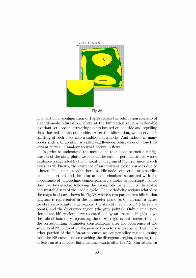
Fig.38

The particular configuration of Fig.38 recalls the bifurcation scenario ofa saddle-node bifurcation, where at the bifurcation value a half-stableinvariant set appear, attracting points located on one side and repellingthose located on the other side. After the bifurcation, we observe thesplitting of such a set into a saddle and a node. And indeed, in manybooks such a bifurcation is called saddle-node bifurcation of closed in-variant curves, in analogy to what occurs in flows.In order to understand the mechanism that leads to such a config-

uration of the state-phase we look at the case of periodic orbits, whoseexistence is suggested by the bifurcation diagram of Fig.37a, since in suchcases, as we known, the existence of an invariant closed curve is due toa heteroclinic connection (either a saddle-node connection or a saddle-focus connection) and the bifurcation mechanisms associated with theappearance of heteroclinic connections are simpler to investigate, sincethey can be detected following the asymptotic behaviour of the stableand unstable sets of the saddle cycle. The periodicity regions related tothe maps in (1) are shown in Fig.39, where a two parameters bifurcationdiagram is represented in the parameter plane (a, k). In such a figurewe observe two quite large regions: the stability region of E∗ (the yellowpoints) and the divergence region (the gray points). Only a small por-tion of the bifurcation curve (pointed out by an arrow in Fig.39) playsthe role of boundary separating these two regions: this means that atthe corresponding parameter constellations after the occurrence of thesubcritical NS bifurcation the generic trajectory is divergent. But in theother portion of the bifurcation curve we see periodicy regions issuingfrom the NS curve, before reaching the divergence region, denoting thatat least an attractor at finite distance exists after the NS bifurcation. In

50

particular, the small regions in different colors correspond to the period-icity regions, each one related to an attracting cycle. The enlargementof two of them (corresponding to attracting cycles of period 4 and 5) isproposed in order to appreciate the fact that they originate below theNS bifurcation curve.

Fig.39 Two parameters bifurcation diagram.

This means that in such a case immediately before the destabilizationof the fixed point two or more attractors coexist. In the generic case,the attracting cycle appears through a saddle-node bifurcation, whichgives also rise to a saddle cycle of the same period, and coexists withthe stable fixed point E∗. The stable set of the saddle cycle separatesthe basins of attraction of the two attractors and the two branches ofthe unstable set reach the fixed point and the attracting node cycle,respectively. Then, at the appearance of the cycles no closed invariantcurves exist, while we know that a repelling closed curve must emergebefore the Neimark-Sacker bifurcation and must shrink, coalescing withthe fixed point at the bifurcation value. How such a curve appears is thequestion we aim to deal.

6.3.1 Saddle-node bifurcation for closed curves

We start our analysis considering the periodicity region in which a cycleof period 4 exists and the particural case of the subfamily of T obtainedby setting a = 0 in (14), that is, the family

T0 =

½x0 = bky + cky2 + dky3 = f (y)y0 = −bx+ cx2 + dx3 = g (x)

(16)

As we have seen in Proposition 1, this is a very particular case sincethe fixed point E∗ undergoes a local bifurcation corresponding to a 1 : 4resonant case, being E∗ a node which bifurcates with pure immaginaryeigenvalues (equal to ±i).

51

The study of the asymptotic behaviour of the maps in (16) can bedeveloped in a simple way once we observe that the maps belonging tothe family T0 are such that T 20 (the second iterate of T0) results in ade-coupled map:

T 20 (x, y) = T0 (f (y) , g (x)) = (f (g (x)) , g (f (y))) = (F (x) , G (y))(17)

Maps having this property, that we shall call “square separate”, havebeen studied in-depth in [20].The main feature is that the dynamic behaviour of the map T0 can be

deduced from the one-dimensional map F (x) (orG (y)) in (17), obtainedby the composition of the two components of T0. Indeed there exists acorrespondence between the cycles of map F (x) and those of T0. Inparticular, if x∗ is a fixed point of F , then (x∗, g (x∗)) is a fixed pointof T0 with eigenvalues6 λ1 =

pF 0 (x∗) and λ2 = −

pF 0 (x∗). If x∗1

and x∗2 are fixed points of F (x) then (x∗1, g (x∗2)) , (x∗2, g (x∗1)) is a cycleof period 2 of T0, with eigenvalue λ1 = F

0(x∗1) and λ2 = F

0(x∗2) . We

deduce that the map T0 has no saddle fixed points, but saddle cyclesmay emerge, for instance when F has two fixed points, one attractingand one repelling.The local bifurcations of the one-dimensional map F correspond to

local bifurcations of T0; indeed, whenever a bifurcation occurs causingthe appearance (disappearance) of cycles of the map F , many cycles ofthe map T0 simultaneously appear (disappear) at the same parametervalues. Such bifurcations of the two-dimensional map are often of par-ticular type, due to the presence of two eigenvalues that simultaneouslycross the unit circle. In particular, a fold bifurcation of a fixed point ofF causes the appearance of two fixed points of T0, one stable and oneunstable, as well as a saddle cycle of period 2.Moreover, we have that a vertical (horizontal) segment is mapped

into a horizontal (vertical) segment by a square separate map and thesame holds for the preimages. Consequently, as the saddle cycles alwayshave eigenvectors parallel to the coordinate axes (see [20]), their unstableand stable sets consist of the union of vertical and horizontal segmentsand the basins of attraction of the different attracting sets are rectangles,if connected, or have many components with rectangular shape.Let us return to the maps we are interested in and consider the one-

dimensional map

F (x) = bk¡−bx+ cx2 + dx3

¢+ck

¡−bx+ cx2 + dx3¢2+dk

¡−bx+ cx2 + dx3¢3

(18)

6In the following, the symbol F 0 (x) denotes the first derivative of F (x).

52

obtained by the composition of the two components of the map T0 in(16). The map F in (18) admits e∗ = 0 as a fixed point and, beingF 0 (0) = −b2k < 0, we obtain that if k < 1/b2 the fixed point is stable.Furthermore, by using a center manifold reduction we obtain that ifdb + c2 + b2c2 − b3d < 0 (and in particular this holds in relation to theparameters we are considering) the bifurcation occurring at k = 1/b2

is a flip of subcritical type7. This means that an unstable cycle r∗ ofperiod 2 exists when the fixed point is still stable and, at the bifurcation,it merges with e∗, leaving an unstable fixed point. Then, we have thatwhen k < 1/b2, the cycle r∗ appears through a fold bifurcation togetherwith a stable one, n∗, of the same period. Then, if the parameter kranges in [ksn, 1/b2], where ksn is the saddle-node bifurcation value, theone-dimensional map F exhibits the coexistence of two attractors, e∗ andthe 2-cycle n∗, whose immediate basins are separated by the periodicpoints of r∗.

Fig.40

Coming back to the two-dimensional map in (16), the above detectedsaddle-node bifurcation of F 2 (the second iterate of F ) causes the suddenappearance of six cycles of period 4 of the map T0, shown in Fig.40b,as described in [20]. Two of these cycles, the attracting node N∗ andthe repelling one R∗, correspond to the cycles n∗ and r∗ respectively.Moreover 4 further cycles of period 4 exist: two of them, the saddles S

∗

and bS∗, due to the coexistence of N∗ and R∗, and two, a stable nodeC∗ and a saddle S∗, due to the coexistence of the cycles N∗ and R∗

with the stable fixed point E∗. Summarizing, as a result of the saddle-node bifurcation of T0 occurring at k = ksn we obtain three coexistingattractors, the fixed point and the period 4 cycles C∗ and N∗, a repelling

7See, for example, Th. 3.5.1 in [50].

53

cycleR∗, and three saddle cycles, S∗, S∗and eS∗. The basins of attraction

of E∗ and C∗ are made up by rectangular components separated by thestable set of the saddle S∗ which gives rise to a heteroclinic connectionwith the periodic points of the repelling cycle R∗. Such a repelling closedcurve bounds the immediate basin of attraction of E∗. The stable setsof the two saddle cycles S

∗and eS∗ separate the basins of attractions of

the two cycles C∗ and N∗ while the unstable ones connect the periodicpoints of the two stable cycles, giving rise to a second invariant closedcurve (see Fig.40b). The two unstable cycles R∗ and S∗ are those alsoinvolved in the flip bifurcation of the fixed point E∗, indeed as the valuek = 1/b2 is approached, the heteroclinic connection between the twocycles shrinks, merging with E∗ at the subcritical bifurcation.Then, starting from the one-dimensional map in (18) we have seen

that two local bifurcations occur for the map T0, a “saddle-node” bi-furcation, giving rise to six cycles of period 4 and a “subcritical flip”bifurcation, at which two of the cycles of period 4, a saddle and a re-pelling node, merge with E∗ leaving an unstable node. The noticeablepoint here is that immediately after the occurrence of the first bifurca-tion two closed curves appear in the phase-space, one attracting, madeup by the unstable sets of the two saddle cycles S

∗and eS∗, and one re-

pelling, made up by the stable set of the saddle cycle S∗, as qualitativelyrepresented in Fig.41b.

Fig.41 Qualitative representation of the "saddle-node" bifurcation for closedcurves

In order to explain such an appearance, we analyze the map at the bifur-cation value k = ksn. At such a value the two cycles N∗ and R∗ coalescein a unique cycle (that we shall callNR∗) as well as the cycles C∗ andN∗

in the cycle CS∗. The Jacobian matrix of T0 evaluated at NR∗ has theeigenvalues equal to ±1 then NR∗ is bifurcating along both the direc-tions of the eigenvectors (eigen-directions for short). Furthermore, dueto the square separate property of T0, the eigen-directions are vertical

54

or horizontal and, consequently, their portions running away from NR∗

must reach the cycle CS∗ (see Fig.41a and Fig.40a). On the other hand,the cycle CS∗ bifurcates with a unique eigenvalue equal to 1, the secondone being smaller than 1 in modulus, and along the eigenvector associ-ated with the eigenvalue 1 the two cycles C∗ and S∗ will appear. Weconclude that at the bifurcation a heteroclinic connection exists betweenthe two cycles CS∗ and NR∗ which surrounds the attracting fixed pointE∗. It attracts the trajectories starting from the external (with respectto the closed curve) portion of the phase-plane and repels those havinginitial condition belonging to the internal one. This is a structurallyunstable situation, which evolves in the appearance of the two invariantclosed curves of Fig.41b.Summarizing, in this first scenario we have seen that the periodic

orbits appear through a saddle-node of codimension 2, that is, to a bi-furcation occurring with two eigenvalues which cross the unit circle at thesame time. This particular situation allows us to obtain, at the bifurca-tion, a half-stable invariant closed curve which is attracting from outsideand repelling from inside. Such a curve can be seen as the merging ofthe two invariant closed curves, one repelling and one attracting, thatappear immediately after the bifurcation. Thus, we observe a saddle-node bifurcation of invariant closed curves, given by the coalescence oftwo closed invariant curves, one attracting and one repelling, followedby their splitting (or their annihilation if the movement of the parame-ters is reversed). Such a bifurcation, quite common in continuous flows,is instead not generic when we deal with two-dimensional maps and itsoccurrence in the map we are considering seems strongly related to oneof the properties of the map itself. We refer, in particular, to the “squareseparate” property, that is, to the fact that the second iterate of the mapresults in a de-coupled map.

6.3.2 Saddle connections

In order to consider a more generic situation we set a = 0.3 and let krange in [5.5713, 5.635], so that the parameters belong to the periodicityregion in which an attracting cycle of period 5 exists. Indeed, at k <5.5713 a saddle-node bifurcation causes the appearance of a stable cycleof period 5 as well as a saddle-cycle of the same period. Immediatelyafter such a local bifurcation no invariant closed curves exist, as shownin Fig.42a where the attracting cycle is turned in a focus C∗, while atk = 5.635 two invariant closed curves exist (see Fig.42b), a repelling oneand a stable heteroclinic connection between the periodic points of thesaddle with those of the attracting cycle, turned into a focus (i.e., theattracting curve is a saddle-focus connection). Looking at the stable and

55

unstable sets of the saddle cycle, we can observe that

• i) the branch of the unstable set converging to the fixed pointE∗ in Fig.42a, after the appearance of the repelling closed curveconverges to the cycle C∗;

ii) both the branches of the stable set of the saddle come from thefrontier of the bounded trajectories in Fig.42a, while in Fig.42b one ofthem exits from the repelling closed curve.

Fig.42

The enlargements in Fig.43 illustrate the different behaviour of the sta-ble and unstable sets of the saddle cycle S∗.

Fig.43

This suggest that the appearance of the repelling closed curve can beexplained by the merging of a branch of the stable set of a saddle cycle Swith a branch of the unstable set of the same cycle. Such a merging gives

56

rise to a structurally unstable closed connection (saddle connection) be-tween the periodic points of S, which develops causing the appearanceof two invariant closed curves, one attracting and one repelling. Themerging of the branches belonging to the stable and unstable sets of thesaddle cycle can be observed around at k = 5.632965625 (see Fig.42c).We summarize in Fig.44a qualitative sketch of this bifurcation. Be-

fore the bifurcation, Fig.44a, an attracting focus cycle coexists with thestable fixed point; the basins of attraction of the two attractors are sep-arated by the stable manifold of the saddle cycle. The unstable branchWU1 = ∪α1,i tends to the fixed point and WU

2 = ∪α2,i to the focus cy-cle. As the bifurcation value is approached, the stable branch ω1,i of thesaddle periodic point Si approaches the unstable branch α1,j of Sj, sopreparing the homoclinic connection. At the bifurcation (Fig.44b) wehave that the two branches ω1,i and α1,j merge giving rise to a connec-tion between the periodic points of the saddle cycle: the attracting cycleis external to such a connection and the branchWU

2 still converges to it.The stable fixed point is internal to the saddle connection which boundsits basin of attraction. Immediately after the bifurcation, an invariantrepelling close curve is created (from which the branch WS

1 comes out,rolling up). The unstable branch WU

1 converges to the focus cycle, cre-ating with WU

2 another closed invariant curve, attracting, given by thesaddle-focus connection (see Fig.44c).

Fig.44

This global mechanism, that does not involve saddle-node bifurcation forclosed curves, neither bifurcations of codimension 2, seems more genericand it has been observed in different models ([6], [3], [5], [7]) and, as weshall see in the next section, it works also when we study the interactionsbetween periodic and quasi periodic trajectories.Moreover a saddle connection may also lead to the appearance of an

attracting closed curve, as shown in ([5]). We illustrate such a mech-anism making use of the qualitative picture in Fig.45 where a pair ofcycles of period 5, a saddle and a repelling focus, is considered.

57

Fig.45

Before the bifurcation, in Fig.45a, a repelling focus cycle and a saddlecycle coexist with the attracting fixed point. The unstable set of the sad-dle cycle converges to E∗ and the two branches of the stable one comefrom different repelling sets: in particular, ω2 issues from the repellingfocus. Approaching the bifurcation, the unstable branch α1, turningaround the periodic points of the repelling focus is closer and closer tothe stable branch ω1. At the bifurcation, these two branches merge, cre-ating a structurally unstable situation given by the saddle connection ofthe periodic points of the saddle cycle (Fig.45b). Immediately after thebifurcation, in Fig.45 c an attracting closed curve Γa appears, surround-ing the periodic points of the cycles, at which converges the unstablebranch α1. At the same time, the stable branch ω1 gives rise with ω2 toa repelling heteroclinic connection with the periodic points of the focuscycle and separates the basins of attraction of E∗ and Γa.Then, we can conclude that if the cycle C, involved in the global bi-

furcation with the saddle S, is attracting then the closed curve appear-ing after the saddle connection is repelling, together with an attractingsaddle-connection. If the cycle C, involved in the global bifurcation withthe saddle S, is repelling then the closed curve appearing after the firststep is attracting, together with a repelling saddle-connection. In par-ticular, in this latter case when the repelling cycle involved in it is anode instead of a focus the two invariant closed curves may appear veryclose to each other, and this is really what is numerically observed whenperforming the study of the dynamical behaviours of the model, as inFig.38.It is worth to observe here that the bifurcations represented in Fig.45c

and Fig.45c are simply a schematic representation. Indeed we are deal-ing with a discrete model and thus it is possible that they occur withan homoclinic tangle, that is in a certain parameter range the contactbetween the stable and unstable set is opened by their quadratic tangen-cies, at which homoclinic orbits appear (and related complex dynamics),followed by transversal intersection and closed by a second quadratictangencies at the opposite side which destroy all the homoclinic orbits.Some examples will be shown in the next section.

58

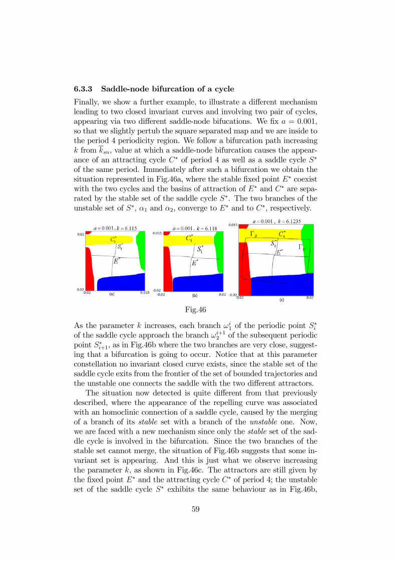
6.3.3 Saddle-node bifurcation of a cycle

Finally, we show a further example, to illustrate a different mechanismleading to two closed invariant curves and involving two pair of cycles,appearing via two different saddle-node bifucations. We fix a = 0.001,so that we slightly pertub the square separated map and we are inside tothe period 4 periodicity region. We follow a bifurcation path increasingk from ksn, value at which a saddle-node bifurcation causes the appear-ance of an attracting cycle C∗ of period 4 as well as a saddle cycle S∗

of the same period. Immediately after such a bifurcation we obtain thesituation represented in Fig.46a, where the stable fixed point E∗ coexistwith the two cycles and the basins of attraction of E∗ and C∗ are sepa-rated by the stable set of the saddle cycle S∗. The two branches of theunstable set of S∗, α1 and α2, converge to E∗ and to C∗, respectively.

Fig.46

As the parameter k increases, each branch ωi1 of the periodic point S

∗i

of the saddle cycle approach the branch ωi+12 of the subsequent periodic

point S∗i+1, as in Fig.46b where the two branches are very close, suggest-ing that a bifurcation is going to occur. Notice that at this parameterconstellation no invariant closed curve exists, since the stable set of thesaddle cycle exits from the frontier of the set of bounded trajectories andthe unstable one connects the saddle with the two different attractors.The situation now detected is quite different from that previously

described, where the appearance of the repelling curve was associatedwith an homoclinic connection of a saddle cycle, caused by the mergingof a branch of its stable set with a branch of the unstable one. Now,we are faced with a new mechanism since only the stable set of the sad-dle cycle is involved in the bifurcation. Since the two branches of thestable set cannot merge, the situation of Fig.46b suggests that some in-variant set is appearing. And this is just what we observe increasingthe parameter k, as shown in Fig.46c. The attractors are still given bythe fixed point E∗ and the attracting cycle C∗ of period 4; the unstableset of the saddle cycle S∗ exhibits the same behaviour as in Fig.46b,

59

reaching both the attractors, but now the basins of attraction of E∗ isbounded by a repelling closed curve ΓU . This closed curve is made upby the stable set of the saddle cycle S∗, now coming from the periodicpoints of a repelling node cycle, R∗, of period 4. The appearance of thecycle R∗ is due to a standard saddle-node bifurcation which gives alsorise to a saddle cycle S of period 4. The stable set of this latter sad-dle cycle separates the basins of attraction of the four fixed points C∗i ,i = 1, 2, 3, 4, of the map T 4, fourth iterate of the map T . The unstableset of the saddle S connects the periodic points of the attracting cycleC∗, so giving rise to an attracting closed curve ΓS. Then, due to theoccurrence of the saddle-node bifurcation, we obtain the appearance oftwo invariant closed curves, one attracting and one repelling, and Fig.47gives a qualitative representation of the mechanism associated with suchan appearance.

Fig.47

We start from a phase space in which an attracting cycle C∗ coexistswith a stable fixed point E∗, the basins of attraction being separatedby the stable set of a saddle cycle S∗, as in Fig.47a. In this frame-work a saddle-node bifurcation of the map T 4 occurs and causes theappearance of a repelling cycle R∗ of period 4 of the map T togetherwith a saddle cycle S of the same period. It is worth to observe thatthe occurring bifurcation is associated with the eigenvalue λ1 = 1 while|λ2| > 1. Then, at the saddle-node bifurcation value, we observe theappearance of a cycle of period 4 (RS in Fig.47b) which is half-stablealong the eigenvector associated with λ1. Along this direction we have astructurally unstable situation, characterized by a branch (the externalone, with respect to a fictitious line joining the periodic points of thecycles) whose points converge to RS while the internal one reaches thesaddle cycle S∗. Furthermore, the eigenvector associated with λ2 has abranch (the external one) converging to the attracting cycle C∗, whilethe internal one belongs to the stable set of the saddle cycle S∗. As a

60

result, we obtain an invariant closed curve, made up by the stable setof the saddle S∗ which connects the periodic points of the cycle RS.Immediately after the bifurcation (Fig.47b) the cycle RS splits up intoa repelling node cycle R∗ and a saddle cycle S; the stable set of thesaddle S∗ persists to give rise to a repelling closed curve, connecting theperiodic points of R∗, and an attracting closed curve appears, made upby the unstable set of the saddle S which connects the periodic pointsof the cycle C∗. Comparing Fig.47b and Fig.41b we remark that thetwo bifurcation mechanisms are quite different, even if both are due toa saddle-node bifurcation of the map T and T0, respectively. Indeed,while in this latter case at the bifurcation value the two invariant curvescoalesce and are half-stable, the sequence commented above gives notthe merging of the two curves, since at the bifurcation a unique hete-roclinic connection exists and is attracting only along a branch of theeigenvector associated with the eigenvalue 1.

6.4 Interaction between invariant closed curves andcycles. A business cycle model

In this section we consider a map T that exhibits some multistabilityphenomena, at least one of the attractor being a closed curve. In suchsituations, the invariant closed curve may interact with the other attrac-tors and interesting dynamic phenomena may occur, often associatedwith homoclinic or heteroclinic tangles. In particular, we shall show twodifferent global bifurcations. The first one causes the transition from onerepelling closed curve to two disjoint repelling closed curves; the secondone causes the transition from an attracting closed invariant curve, sayΓa, with a pair of cycles of period k outside it, a saddle S and an attract-ing one, C, to a wider attracting closed invariant curve, say Γb, with thetwo cycles inside it.In order to illustrate the mechanisms associated with these phenom-

ena, we consider the following discrete-time version of the Kaldor non-linear model of the business cycle½

Yt+1 = Yt + α (It − (Yt − Ct))Kt+1 = It + (1− δ)Kt

(19)

where the dynamic variables Yt and Kt represent the income (or output)level and the capital stock in period t, respectively, and both the invest-ment It and the consumptionCt (or equivalently the savings St = Yt−Ct)are assumed to depend in general on Yt and Kt.The first equation in (19) views the output level as reacting over time

to the excess demand or, put differently, to the difference between ex-ante investment (It) and saving (St = Yt−Ct). The speed of adjustment

61

is measured by the parameter α (α > 0), where a value of α smaller than1 means a prudent reaction by firms, while a value of α greater than 1denotes rash reactions and coordination failure.The second equation in (19) models the capital stock as being in-

creased by realized investment (here assumed to coincide with ex-anteinvestment) It = It (Kt, Yt), and decreased by depreciation δKt, where δ(0 < δ < 1) represents the capital stock depreciation rate.The discrete dynamical equations (19) (or, alternatively, their continuous-

time counterparts) provide the common structure of several versions ofthe Kaldor model, which have been proposed in the literature up to now(see [33], [57], [48], [23], [8], [10] among others), and a different examplewill be also shown below in Section*. Such models are able to produceboth periodic or quasi-periodic trajectories and further dynamic scenar-ios, ranging from chaotic fluctuations to coexistence of different attrac-tors, once the investment and the savings function It and St are specifiedin a way consistent with Kaldor’s original qualitative assumptions.The assumptions about consumption (Ct) and investment (It), which

are the same as in [57], [74] and [8], are

• ConsumptionAt each time t, the consumption is a nonlinear sigmoid shapedfunction of income:

Ct = c0 +2

πc1 arctan

µπc22c1

(Yt − Y ∗)¶

(20)

where Y ∗ denotes the exogenously assumed equilibrium (or nor-mal) level of income and c0, c1, c2 are positive parameters. Theconsumption is therefore an increasing function of income (rangingbetween c0 − c1 and c0 + c1): however, while for extreme valuesof income consumption remains nearly constant, i.e. the fractionof income spent for consumption decreases as income increases,there exists a region around the normal level Y ∗ where consump-tion increases rapidly at a rate close to c2, which represents theconsumption propensity at Y ∗ (we assume 0 < c2 < 1). Theconsumption function (20), or equivalently the inverted S-shapedsavings function St = Yt−Ct, reflects the view that the proportionof income which is saved is higher in non-ordinary periods, whenYt is far from Y ∗, because in such periods people perceive a largerportion of their income as being transitory.

• Investment

62

At each time t, the investment is a linear function of income andcapital stock. Precisely it is assumed that (gross) investment re-sponds to a gradual adjustment of the actual capital stock to thedesired capital stock

It = b¡Kd

t −Kt

¢+ δKt

whereKdt is the desired stock of capital at time t, which is assumed

linear in current output,Kdt = kYt, k represents the desired capital-

output ratio (which will be considered as an exogenous parameterhere) and b, 0 < b < 1, is the capital stock adjustment parameter.Therefore the investment function can be rewritten as a linearfunction of income and capital, as follows

It = bkYt − (b− δ)Kt (21)

where the Kaldorian negative relation between investment and cap-ital stock is fulfilled provided that b > δ.

Substituting the consumption and investment functions (20)-(21) inmodel (19) we get(Yt+1 = (1− α+ αbk)Yt + α

³c0 +

2πc1 arctan

³πc22c1(Yt − Y ∗)

´− (b− δ)Kt

´Kt+1 = b (kYt −Kt) +Kt

(22)from which the coordinates of the exogenous fixed point can be easilyobtained ½

Y ∗ = c01−kδ

K∗ = kY ∗ = kc01−kδ

In order to simplify the analysis of the model (22), we normalize thefixed point to (0, 0), by reformulating the model in terms of deviations½

xt = Kt − kY ∗

yt = Yt − Y ∗(23)

With the new coordinates (23), the dynamical system (22) is representedby the following map

T :

(x0 = (1− b)x+ bky

y0 = α (δ − b)x+ (1− α+ αbk) y + 2παc1 arctan

³πc22c1

y´ (24)

Note first that the map T is independent on c0, which means that c0 isonly a “location” parameter and does not affect the asymptotic behav-iour of the system. Second, though the map T depends on 6 parameters,

63

in our analysis we will assume b, k, δ, c1 as fixed parameters, and wewill perform stability and bifurcation analysis in the parameter space

Ω = (α, c2) : α > 0 and 0 < c2 < 1

The properties of the map T in (24) are studied in [8], at which theinterested reader is addressed for major details. We only recall here thesymmetric property of T , whose implications is that any invariant set ofT either is symmetric with respect to the origin, or it admits a symmetricinvariant set, and the existence of a region in the parameter space wherethe map is not invertible (being a Z1 − Z3 − Z1 map). In our analysiswe shall consider a parameter range in which T is invertible. Even theexistence of the fixed points and the local stability of the exogenousfixed point (obtained as usual by the localization of the eigenvalues ofthe Jacobian matrix) is performed in [8] and we only recall the mainresults:

Proposition 2 The map T in (24) has

• the unique fixed point E∗ = (0, 0), if c2 ≤ 1− kδ or 1− δk ≤ 0• three fixed points, E∗ = (0, 0) and two further points, P ∗ and Q∗,symmetric with respect to E∗, if c2 > 1− kδ > 0.

Proposition 3 Assume δk < 1, b < 1.

• If b > δ and (2− b)2 > bk (4− 4δ + δb) the fixed point E∗ =(0, 0) is locally asymptotically stable if the parameters α and c2belong to the region OABCD of the plane (α, c2), with vertices

O = (0, 0), A =³

2(2−b)2−b−bk(2−δ) , 0

´, B =

³(b−2)2bk(b−δ) ,

(2−b)2−bk(δb−4δ+4)(−2+b)2

´,

C =³

bk(b−δ) , 1− δk

´, D = (0, 1− δk), where the sides AB, BC

and CD belong to the hyperbola of equation

c2 = c2f (α) =α− 2α− bk (2− δ)

2− b(25)

to the hyperbola of equation

c2 = c2N (α) = 1 +b− αbk (1− δ)

α (1− b)(26)

an to the line c2 = 1− δk, respectively;

64

• if b > δ and (2− b)2 < bk (4− 4δ + δb) the fixed point E∗ = (0, 0)is locally asymptotically stable if the parameters α and c2 belongto the region OBCD of the plane (α, c2), with vertices O = (0, 0),

B =³

bbk(1−δ)−(1−b) , 0

´, C =

³b

k(b−δ) , 1− δk´, D = (0, 1− δk),

where the sides BC and CD belong to the hyperbola of equation

c2 = c2N (α) = 1 +b− αbk (1− δ)

α (1− b)

an to the line c2 = 1− δk, respectively;

• if b < δ the fixed point E∗ = (0, 0) is locally asymptotically sta-ble if the parameters α and c2 belong to the region OABD of theplane (α, c2), with vertices O = (0, 0), A =

³2(2−b)

2−b−bk(2−δ) , 0´, B =³

2−bk(δ−b) , 1− δk

´, D = (0, 1− δk), where the sides AB and BD be-

long to the hyperbola of equation

c2 = c2f (α) =α− 2α− bk (2− δ)

2− b

an to the line c2 = 1− δk, respectively.

Moreover if the point (α, c2) exits the stability region by crossingthe side AB, then a supercritical flip bifurcation occurs at whichE∗ becomes a saddle point and a period 2 attracting cycle appears;if the point (α, c2) exits the stability region by crossing the sideBC, then a Neimark bifurcation occurs at which E∗ is transformedfrom a stable focus to an unstable focus and an attracting closedinvariant curve appears around it; if the point (α, c2) exits the sta-bility region by crossing the side CD, then a supercritical pitchforkbifurcation at which two stable fixed points are created close to E*,which becomes a saddle.

In the following we shall consider δ ≤ b, so that self-sustained oscilla-tory behavior around the unstable fixed point E∗ occur, and (2− b)2 <bk (4− 4δ + δb). In this parameter region the exogeneous fixed point canbe destabilized only via pitchfork bifurcation or via a NS bifurcation andwe shall follow a bifurcation path starting from a point correspondingto two stable fixed points P ∗ and Q∗ and an unstable fixed point E∗, lo-cated in the middle, i.e. a situation of bi-stability (without oscillations),and moving towards a region where self-sustained oscillations exist (seeFig.48).

65

Fig.48

However, our global analysis will point out that long-run oscillatory be-havior is possible even for high values of c2 (beyond the pitchfork bound-ary), in parameter ranges where two further equilibria P ∗ and Q∗ existand are stable, or where they exist unstable but further stable periodicorbits exist. This will reveal phenomena of coexistence of the Kaldorianbusiness cycle with other possible long-run dynamic outcomes, wherethe role played by the initial condition will be crucial.

6.4.1 From one repelling closed curve to two repelling ones

Immediately after the pitchfork bifurcation of the exogenous fixed pointE∗, two attracting fixed points, the nodes P ∗ and Q∗, appear, locatedat symmetric positions with respect to the saddle E∗. Their basins ofattraction are separated by the stable manifold W S (E∗). The unstableset WU (E∗) reaches the two fixed points: more precisely, a branch, sayα1, tends to P ∗ whereas the other one, say α2, goes to Q∗.The phase portrait of Fig.49a shows an example of this situation:

it has been obtained at α = 1.5 and c2 = 0.98, then quite far fromthe bifurcation. Indeed at this parameter values the two nodes haveturned into stable foci and the stable set of the saddle exhibits someconvolutions separating the basins of attraction of P ∗ and Q∗, B (P ∗)and B (Q∗) respectively, represented in red and gray respectively.As the speed of adjustment α increases, the set WS (E∗) involves

more and more, winging around the fixed points P ∗ and Q∗, as shown inFig.49b. Consequently, the basin boundary appear to be more compli-cated and a trajectory starting from the region where the convolutionsget thicker is subject to greater uncertainty about its long run behav-iour. In fact, a slight perturbation of an initial condition taken in sucha region may cause a crossing of the basin boundary and consequentlythe convergence to a different equilibrium.

66

Fig.49

Moreover this basin structure suggests that some global bifurcation isabout to occur. Indeed, when α is slightly increased, as in Fig.50a, anattracting closed curve Γ appears in the area where there was manyconvolutions of W S (E∗). This means that long-run quasi-periodic self-sustaining fluctuations are now a possible outcome, as well as dampenedoscillations converging to the fixed points: three typical trajectories,starting from initial condition taken in the three different basins, arerepresented versus time in Fig.50b.

Fig.50

The basins of attraction of P ∗ and Q∗ are still separated by the stablemanifold of the saddle E∗, but, differently from the case illustrated inFig.49, now the preimages of the points of WS (E∗) accumulate on a re-pelling closed curve eΓ, appeared with Γ and very close to it (see Fig.50).The appearance of Γ and eΓ could be due in principle to a “saddle-node”bifurcation for closed curves, given that the two curves are very closeeach other, but we know that such a bifurcation is very infrequent in

67

discrete maps. Then a mechanism similar to that described in the pre-vious section may be conjectured in this case: a saddle cycle appearsvia saddle-node together with a repelling (attracting) node cycle of thesame period, then a saddle connection made up by the merging of twobranches of the stable and unstable manifolds of the saddle gives riseto an attracting (repelling) closed invariant curve and to a heteroclinicconnection between the periodic points of the two cycles made up bythe stable (unstable) set. These two invariant closed curves appear veryclose to each other and if the period of the cycle is very high they looklike those of Fig.50a.Whatever be the underlying mechanism, the appearance of the two

invariant closed curves, one attracting and one repelling, has a noticeableeffect on the asymptotic behaviour of the model, since three attractorsnow coexist (the two equilibria, P ∗and Q∗, and the closed curve Γ), thebasins B (P ∗) and B (Q∗) are strongly reduced and the majority of thetrajectories are quasi-periodic (or periodic of very high period), sincethe curve eΓ is now the basin boundary of Γ.Moreover the repelling closed curve eΓ is involved in other important

qualitative change in the structure of the basins of attraction as theadjustment speed is increased further. Indeed, as we can see in Fig.51a,it progressively reduces in size and shrinks in proximity of the saddle E∗.Up to now, initial conditions taken close to the exogenous equilibriumgive rise to trajectories converging to P ∗ or Q∗, but this is not true inthe parameter constellation of Fig.51c, where trajectories starting closeto E∗ exhibit self-sustaining oscillations.

Fig.51

This means that the points of the unstable manifold ofE∗ no longer reach

68

the two equilibria but converge to Γ. This change in the asymptoticbehaviour of WU (E∗) proves that a global bifurcation has occurred,involving both the unstable branches of the saddle E∗. Indeed in thephase portrait of Fig.51b we can observe the splitting of eΓ into tworepelling closed curves, ΓP and ΓQ, each one bounding the basin ofthe corresponding fixed point. These two repelling closed curves arethe α-limit sets of the points of the two branches ω1 and ω2 of thestable set WS (E∗), which have modified their behaviour as well. Thenwe deduce that when the parameter α ranges from 1.568 to 1.57, ahomoclinic bifurcation of E∗ occurs, whose effect is the transition fromone “big” repelling closed curve, basin boundary of the attracting setP ∗, Q∗, to two “small” repelling closed curves, basin boundaries ofB (P ∗) and B (P ∗) respectively. This situation can be classified as adouble homoclinic loop, since it involves both the branches of the stableand unstable sets of the saddle E∗: its evolution is represented in Fig.52,where some enlargements of the phase space as well as of the stable andunstable sets of E∗ are shown.

Fig.52

The first homoclinic tangency is shown in Fig.52a,b, obtained at α =1.56855: the branch α1 of WU (E∗) converges to P ∗ and it is completelycontained in its basin of attraction; the same is true for α2 with respectto the fixed point Q∗. The stable branches have a complex structure:the repelling closed curve Γ is replaced by a strange repellor, generatedby the tangency and separating the basins of P ∗, Q∗ and Γ. After thetransversal crossing of WS (E∗) and WU (E∗) , at which more and more

69

homoclinic points of E∗ are created, the second homoclinic tangencyoccurs at α = 1.5685501, as shown in Fig.52c,d, and closes the tangle.The homoclinic points of E∗ disappear as well as the chaotic repellor,leaving the two disjoint curves ΓP and ΓQ as boundaries of the basins ofattraction of P ∗ and Q∗, respectively. After the homoclinic tangle boththe branches of WU (E∗) converge to the attracting closed curve Γ andthose of the stable set WS (E∗) come from the repelling closed curve ΓPand ΓQ.A different illustration of this homoclinic tangle, occurring in a very

narrow parameter α range, is proposed in Fig.53, where we show theasymptotic behaviour of the whole unstable set of the saddle E∗. InFig.53a, obtained at the same parameter value as Fig.53a correspondingto the first homoclinic tangency, the points of WU (E∗) converge to thetwo equilibria, forming an eight-shaped structure; then, in Fig.53b theunstable set WU (E∗) enters the basin of attraction of the attractingclosed curve Γ as well as that of the attracting set P ∗, Q∗: the sep-arator of the three basins of attraction is a chaotic repellor, associatedwith the infinitely many periodic points existing close to the homoclinictrajectories. As α is further increased, more and more points ofWU (E∗)converge to Γ until at the second homoclinic tangency, shown in Fig.53c,no points of the unstable set converge to the two stable foci.

Fig.53

As the parameter α further increases, the two repelling closed curvesΓP and ΓQ become smaller and smaller, until a new bifurcation valueα = eαN is reached at which a Neimark subcritical bifurcation occurs:

70

the two repelling closed curves collapse in P ∗ and Q∗ respectively and atα > eαN the attracting closed curve Γ is the unique surviving attractor,since the two fixed points become unstable foci.

6.4.2 Interaction between coexisting invariant curve and cy-cles.

After the subcritical Neimark bifurcation of P ∗ andQ∗, the saddleE∗ co-exists with two repelling foci, from which the stable set W S (E∗) comes.The points of the unstable manifoldWU (E∗) converges to the attractingclosed curve Γ surrounding the three unstable fixed points.This situation persists until at a certain value of α, say αsn, a saddle-

node bifurcation occurs, causing the appearance of two cycles of period8, a saddle, S, and a stable node, C , which turns into a stable focus cy-cle immediately after. The two cycles are located outside the attractingclosed curve and, as α increases from αsn, a larger and larger portionof trajectories exhibits period-8 oscillations, as shown in Fig.54a, wherethe basins of attraction of the two attractors are represented in yellowand light blue. The points close to the endogenous equilibrium E∗ stillgive rise to quasi-periodic fluctuations.

Fig.54

The phase portrait shown in Fig.54b is completely different: quasi-periodic and period-8 trajectories still coexist, but now the attractingclosed curve eΓ surrounds the stable focus cycle C and the majority of

71

the trajectories exhibit quasi-periodic motion. Moreover the long runbehaviour of trajectories starting in the area close to E∗ is no longerpredictable, since a small shock on them may have strong consequencesgiven the many and many convolution of the separatrix of the two basinsin this area.The global mechanisms which cause this important modification in

the basin structures, transforming an attracting closed curve, coexist-ing with a stable cycle external to it, in a larger one, surrounding it,has to involves the stable and unstable sets of the saddle, since theychange behaviour. Indeed, in Fig.54a, obtained at α = 1.7 > αsn, twoattractors exist, the closed curve Γ and a focus cycle C, surrounding thecurve, while the two basins, B (C) and B (Γ), are separated by the stablemanifold W S (S) = ω1 ∪ ω2 of the saddle S. Both the branches of thestable manifold have as α-limit set the frontier of the set of boundedtrajectories. The branches of the unstable one WS (S) reach the at-tracting closed curve (α1) and the stable focus cycle (α2). While, inFig.54b, two attractors still exist, the closed curve Γ and the focus cycleC, surrounded by the curve; the stable manifold of the saddle cycle stillseparate the basins of attraction of the two attractors, but its α-limitset now belongs to the attracting set given by the three fixed points.Moreover, the branches of the unstable one play the opposite role, α1reaching the stable focus and α2 the attracting closed curve. Then, tounderstand the bifurcation, we follow these invariant sets, increasingslowly the parameter α.

Fig.55

As the parameter α is increased, the two branches ω1 and α1 start tooscillate until a homoclinic tangency occurs. More precisely, at α =1.7102384 the stable branch α1,i of the periodic point Si has a tangen-tial contact with the unstable branch ω1,j of a different periodic pointSj (see Fig.55a) and this occurs cyclically for all the periodic points ofthe saddle S. This contact is the starting point of a heteroclinic tangle,which develops in a transversal crossing of the involved inner branches

72

(Fig.55b) and closes at α = 1.7102387, at which value a second cyclicalhomoclinic tangency occurs (Fig.55c). Observe that at the end of theheteroclinic tangle, the two branches α1 and ω1 (but not α2 and ω2) haveexchanged they reciprocal position with respect to Fig.55a. Approachingthe heteroclinic tangle, the curve Γ exhibits more and more oscillations,as in Fig.56a obtained at the same parameter values of Fig.55a, beforeits disappearance. Moreover during the tangle a chaotic repellor R iscreated in the area occupied by the transversal crossing of the two man-ifolds. The presence of the chaotic repellor can be detected by lookingthe map T 8 and, in particular, to the basins of attraction of its 8 sta-ble fixed points given by the periodic points of the attracting cycle C.As we show in Fig.56b, such basins, well separated in a portion of thephase-space, are instead strongly intermingled in the area occupied bythe transversal crossing of the two manifolds, denoting the existence ofinfinitely many repelling cycles which cause an erratic behaviour of thetrajectories converging to the different fixed points.

Fig.56

The existence of the R has important effects on the long run behaviourof the trajectories starting from the area occupied by the chaotic repel-lor, since they have a very long transient part before to reach the period8 oscillations.The effects of the observed heteroclinic tangle are illustrated in Fig.57:

the attracting closed curve Γ disappears, or better, it comes into reso-nance with the cycle, forming an attracting set with the saddle S andthe focus cycle C, with C the attractor within it. leaving the focus cycleC as unique attractor (Fig.57a). More precisely, Γ has been replaced bythe heteroclinic connection of the periodic points of the cycles, made up

73

by the unstable manifold of the saddle S which reach the periodic pointsof the focus cycle (Fig.57b).

Fig.57

With a similar mechanism the final situation of Fig.54b is obtained.Indeed, increasing α the two outer branches α2 and ω2 approach eachother, oscillating. This is the prelude to a new heteroclinic tangle, stilloccurring in a very small range of the parameter α: the first tangen-tial contact between the unstable branch α2,i of the periodic point Siand the stable branch ω2,j of a different periodic point Sj is followed bytheir transversal crossing and then by the homoclinic tangency occurringat the opposite side with respect to the previous one (as illustrated inFig.58).

Fig.58

In the area occupied by the transversal crossing of the invariant sets, achaotic repellor appears at the first homoclinic tangency (see Fig.59a),

74

persists during the transversal crossing phase and disappears at the clos-ing of the tangle: consequently, the trajectories starting close to it havea longer transient part before converging to the period 8 cycle. But themain effect of this global bifurcation is the appearance of an attractingclosed curve eΓ, which replaces the heteroclinic connection between theperiodic points of the cycles S and C. As soon as it has appeared, itexhibits many oscillations, as shown in Fig.59b obtained at the sameparameter value as Fig.58c, and surrounds the periodic points of theattracting cycle. As α increases, eΓ becomes smoother and smootherreaching the shape of Fig.54b.

Fig.59

To sum up, we qualitatively describe the sequence of bifurcations caus-ing the transition from an attracting closed invariant curve with a pairof cycles outside it, a saddle and an attracting one, into another widerattracting closed invariant curve, occurring via heteroclinic loops of thesaddle. Let us consider the situation described in Fig.60. In Fig.60a wehave an attracting closed invariant curve Γa, and a pair of cycles thathave been created via a saddle-node bifurcation outside Γa. Such ex-ternal cycles do not form an heteroclinic connection, whereas the stableset of the saddle S bounds the basin of attraction of the related attract-ing fixed points Ci of the map T k. The unstable branches α1,i of Sitend to the attracting curve Γa, while the unstable branches α2,i of Sitend to the attracting cycle. At the bifurcation (Fig.60b) we may havethat the closed invariant curve Γa merges with the unstable branchesWU1 (S) = ∪α1,i and with the stable ones WS

1 (S) = ∪ω1,i as well, in aheteroclinic loop, or tangle, of the saddle S, causing the disappearanceof the attracting closed invariant curve Γa, and leaving another closedinvariant curve, see Fig.60c, which is now the heteroclinic connection

75

Figure 1: Fig.60

involving the saddle S and the related attracting cycle C. After thebifurcation of the heteroclinic loop a closed curve still exists, but differ-ently from Γa it includes the two cycles on it (Fig.60c).Starting from this situation, a second heteroclinic loop (or tangle)

may be formed. The heteroclinic connection turns into a heteroclinicloop in which the unstable branches WU

2 (S) = ∪α2,i merge with thestable ones WS

2 (S) = ∪ω2,i (see Fig.60d). After the bifurcation a newclosed attracting curve exists, say Γb, and the two cycles are both insideΓb (Fig.60e). The stable set of the saddle S separates the basins ofattraction of the k attracting fixed points Ci of the map T k. The unstablebranches ∪α1,i tend to the attracting cycle while the unstable branches∪α2,i tend to Γb.As we have seen, in the case of discrete dynamical systems, the dy-

namic behaviors more frequently observed is such that the heteroclinicloop of Figs.60b,d are replaced by homoclinic tangles. That is, a tangencyoccurs between the two manifolds involved in the bifurcation, followedby transverse intersections and a tangency again on the opposite side,after which all the homoclinic points of the saddle S, existing during thetangle, are destroyed.It is worth noticing that all the unstable periodic points associated

with the first homoclinic tangle, due toWU1 (S)∩WS

1 (S) 6= ∅, are in theregion interior to the set of periodic points of the saddle S, whereas in thestrange repellor associated with the second homoclinic tangle, in whichWU2 (S) ∩WS

2 (S) 6= ∅, all the unstable cycles are “outside” the saddle

76

cycle S. Notice also that before the first heteroclinic loop (tangle) ofFig.60 we have two distinct attracting sets: Γa and the stable k−cycleoutside it; after the second one of Fig.60, we have again two distinctattractors: Γb, which is wider than Γa, and the k−cycle inside it, whilebetween the two heteroclinic loops only one attractor may survive, thatis the k-cycle.

77

7 Basin of attraction and related contact bifurca-tions.

In this section we recall some definitions and properties associated withthe basins of attractiong sets. Let us consider an m−dimensional mapx0 = T (x) and an invariant attracting set A ⊂ Rm (thus it is mappedinto itself, T (A) = A, i.e. if x ∈ A then Tn(x) ∈ A for any n > 0). Asalready defined, the Basin of attraction of A is the set of all the pointsthat generate trajectories converging to A

B (A) = x|T n(x)→ A as n→ +∞ . (27)

Starting from the definition of attracting set, let U(A) be a neighborhoodof a A whose points converge to A. Of course U(A) ⊆ B (A), but notethat also the points of the phase space which are mapped inside U aftera finite number of iterations belong to B (A). Hence, the total basin ofA (or briefly the basin of A) is given by

B (A) =∞[n=0

T−n(U(A)), (28)

7.1 One-dimensional mapsLet us start with one-dimensional, continuous and noninvertible maps, towe illustrate how non-connected basins of attraction arise. Furthermore,we show how the global bifurcations that cause their qualitative changescan be described in terms of contacts between critical points and thebasins’ boundaries.Let us first take a look at iterated invertible maps though. If f :

I → I is a continuous and increasing function, then the only invariantsets are the fixed points (as already remarked in Section 1). When manyfixed points exist, say x∗1 < x∗2 < ... < x∗k, they are alternatingly stableand unstable: the unstable fixed points are the boundaries that separatethe basins of the stable ones. Starting from an initial condition wherethe graph of f is above the diagonal, i.e. f(x0) > x0, the generatedtrajectory is an increasing sequence converging to the stable fixed pointon the right, or it is diverging to +∞. On the other hand, starting froman initial condition such that f(x0) < x0, the trajectory is a decreasingsequence converging to the fixed point on the left, or it is divergingto −∞ (see Fig.61a, where p∗ is a stable fixed point, and its basin isbounded by two unstable fixed points q∗ and r∗, where q∗ < p∗ andr∗ > p∗). If f : I → I is a continuous and decreasing map, the onlypossible invariant sets are one fixed point and cycles of period 2. Periodicpoints of the cycles of period 2 are located around the fixed point, the

78

unstable ones being boundaries of the basins of the stable ones (seeFig.61b, where a stable fixed point x∗ exists, and its basin is boundedby the periodic points α1, α2 of an unstable cycle of period 2).

Fig.61

In general, in the case of one-dimensional invertible maps the only kindsof attractors are fixed points and cycles of period two. In the first case,the basin is an open interval which includes the fixed point, and inthe second case, the basin is the union of two open intervals, each oneincluding an attracting periodic point.Obviously, if the map is invertible, the basins of the attracting sets are

simple. This may be no longer true if the map is noninvertible. In thiscase the structure of a basin may be very complicated. Non-connectedportions of the basins may be created, given by open intervals that donot include any point of the related attractor. As a first example, let usconsider the logistic map (3) (Fig.8 of Section2), a noninvertible Z0−Z2map whose graph is represented again in Fig.62.

Fig.62

For µ < 4 every initial condition x0 ∈ (0, 1) generates bounded se-quences, converging to a unique attractor A (which may be the fixed

79

point x∗ = (µ− 1) /µ or a more complex attractor, periodic or chaotic).Initial conditions out of the interval [0, 1] generate sequences diverging to−∞. The boundary that separates the basin of attraction B (A) of theattractor A, from the basin B (∞) is formed by the unstable fixed pointq∗ = 0 and its rank-1 preimage (different from itself), q∗−1 = 1. Observethat, of course, a fixed point is always preimage of itself, but in this casealso another preimage exists because q∗ ∈ Z2. If µ < 4, as in Fig.62a,then q∗−1 > c = µ/4, where c is the critical point (maximum) that sep-arates Z0 and Z2. Hence, q∗−1 ∈ Z0. When we increase µ, at µ = 4we have q∗−1 = c = 1, and a contact between the critical point and thebasin boundary occurs. This is a global bifurcation, which changes thestructure of the basin (really it destroys the basin). For µ > 4 (Fig.62b)we have q∗−1 < c, and the portion

¡q∗−1, c

¢of B (∞) enters Z2. This

implies that new preimages of that portion are created, which belongto B (∞) according to (28). As we know, almost everything will thenbelong to the basin of divergent trajectories, the only points which areleft on the interval I are the points belonging to the chaotic invariantset Λ, as described in Section 2 (on which the restriction of the map isstill chaotic).A similar situation occurs for a unimodal Z0 − Z2 map where the

attractor at infinity is replaced by an attracting fixed point, as the oneshown in Fig.63a. As in the previous example, we have an attractor A,which may be the fixed point x∗ (or some other invariant set around it),with a simply connected basin bounded by the unstable fixed point q∗

and its rank-1 preimage q∗−1. This example differs with respect to theprevious one in so far as in this case initial conditions taken in the com-plementary set generate trajectories converging to the stable fixed pointz∗. This means that the basin B (z∗) is formed by the union of two non-connected portions: B0 = (−∞, q∗) ⊂ Z2, which contains z∗ (it is usuallycalled immediate basin, the largest connected component of the basinwhich contains the attractor) and B1 =

¡q∗−1,+∞

¢= f−1 (B0) ⊂ Z0. In

Fig.63a the two non-connected portions of the basin B (z∗) are marked bybold lines. Interesting effects occur, if some parameter variation causesan increase of the critical point c (maximum value) until it crosses thebasin boundary q∗−1. If this happens, the interval (q

∗−1, c), which is part

of B1, enters Z2, and infinitely many non-connected portions of B (z∗)emerge in the interval (q∗, q∗−1). Note that the total basin can still beexpressed as the union of all the preimages of any rank of the immediatebasin B0.

80

Fig.63

Another interesting situation is obtained if we change the right branch ofthe map of Fig.63a by folding it upwards such that another critical point,a minimum, is created. Such a situation is shown in Fig.63b. This is anoninvertible Z1−Z3−Z1 map, where Z3 is the portion of the codomainbounded by the relative minimum value cmin and relative maximum valuecmax. In the situation shown in Fig.63b we have three attractors: thefixed point z∗, with B (z∗) = (−∞, q∗), the attractor A around x∗, withbasin B (A) = (q∗, r∗) bounded by two unstable fixed points, and +∞(i.e. positively diverging trajectories) with basin B (+∞) = (r∗,+∞).In this case all the basins are immediate basins, each being given by anopen interval. In the situation shown in Fig.63b, both basin boundariesq∗ and r∗ are in Z1, so they have only themselves as unique preimages(like for an invertible map). However, the situation drastically changesif, for example, some parameter changes causes the minimum value cminto move downwards, until it goes below q∗ (as in Fig.63c). After theglobal bifurcation, when cmin = q∗, the portion (cmin, q∗) enters Z3, sonew preimages f−k (cmin, q∗) appear with k ≥ 1. These preimages con-stitute non-connected portions of B (z∗) nested inside B (A), and arerepresented by the thick portions of the diagonal in Fig.63c.

7.2 Two-dimensional maps.To better understand the subject, we consider a first example takenfrom Bischi and Kopel [22]: a dynamic duopoly game in the tradition ofCournot. In contrast to the early models on oligopoly dynamics, in theirmodel players form adaptive expectations and players’ reaction functionsare unimodal. This framework gives rise to a situation of multistability,where the basins of each stable Nash equilibrium is a rather complicatedset. The second example presents a dynamic brand competition modelproposed by Bischi, Gardini and Kopel [21]. In this game a unique andstable fixed point exists, but the basin of the fixed point can have a verycomplicated structure. Several other examples may be fowd in [89], [2],[96], [97].

81

7.2.1 Example 1: Quantity-setting duopoly games with adap-tive expectations

The first example we present is a dynamic Cournot duopoly game withunimodal reaction functions. The two quantity-setting firms produce ho-mogeneous goods and, since they do not know the competitor’s output,they try to predict this quantity using an adaptive scheme. Let x1 (t)and x2 (t) be the outputs at time period t. The two players determinetheir production quantities of the next period, x1 (t+ 1) and x2 (t+ 1),by solving the optimization problems

Maxx1

Π1 (x1, xe2(t+ 1)) ; Max

x2Π2 (x

e1(t+ 1), x2) (29)

where Πi is the profit of player i, and xei (t + 1), i = 1, 2 represent thepredictions for the output of the competitor. The solutions of the opti-mization problems (assumed to be unique) are denoted by

x1 (t+ 1) = r1 (xe2(t+ 1))

x2 (t+ 1) = r2 (xe1(t+ 1))

(30)

where r1 and r2 are called the Best Replies (or reaction functions). In theoriginal work of Cournot [26], as well as in much of the literature whichfollowed, naive expectations xei (t+ 1) = xi (t) have been considered.Under the assumption of naive expectations each firm expects or predictsthat the quantity offered by the competitor in the next period will bethe same as in the current period. The time evolution of the duopolysystem is then represented by the two-dimensional discrete dynamicalsystem

(x1 (t+ 1) , x2 (t+ 1)) = (r1 (x2 (t)) , r2 (x1 (t))) (31)

which is also referred to as the Cournot tâtonnement process. In contrastto this, in Bischi and Kopel [22] firms are assumed to revise their beliefsaccording to the adaptive expectations scheme

xe1 (t+ 1) = xe1 (t) + α1 (x1 (t)− xe1 (t))xe2 (t+ 1) = xe2 (t) + α2 (x2 (t)− xe2 (t))

(32)

If the relations (30) are inserted into (32), one gets the following two-dimensional dynamical system in the belief space

xe1 (t+ 1) = (1− α1)xe1 (t) + α1r1 (x

e2 (t))

xe2 (t+ 1) = (1− α2)xe2 (t) + α2r2 (x

e1 (t))

. (33)

Of course, the quantities chosen by the competitors can be obtained bythe transformations x1 (t) = r1 (x

e2 (t)), x2 (t) = r2 (x

e1 (t)), i.e. by a

82

mapping from the belief space into the action space. The fixed points ofthe dynamical system (33), defined by xei (t+ 1) = xei (t), i = 1, 2, i.e.

xe1 (t) = r1 (xe2 (t))

xe2 (t) = r2 (xe1 (t))

(34)

are located at the intersections of the two reaction curves and are inde-pendent of the adjustment coefficients α1 and α2. In other words, a fixedpoint is a situation where beliefs are not further revised and quantities donot change, and at the fixed points the expected outputs coincide withthe realized ones. Hence, in belief space we are considering a situationwhere beliefs are consistent and this corresponds to a Nash equilibriumin the quantity space. In Bischi and Kopel [22] the following reactionfunctions have been considered

r1(x2) = µ1x2 (1− x2)r2(x1) = µ2x1 (1− x1)

(35)

It has been shown elsewhere (see Kopel, [69]) that if the competitorsregard their products as strategic complements over a certain range ofthe set of admissible actions, the functions given in (35) can be derivedas Best Responses, and the parameters µi, i = 1, 2 measure the intensityof the positive externality the actions of one player exert on the payoffof the other player.To simplify the notation, we rename the expected outputs by setting

x(t) = xe1 (t) and y(t) = xe2 (t). Inserting the reaction functions specifiedin (35) into (33), the time evolution of the competitors’ beliefs is obtainedby the iteration of the two-dimensional map T : (x, y)→ (x0, y0) definedby

x0 = (1− α1)x+ α1µ1y (1− y)y0 = (1− α2) y + α2µ2x (1− x)

(36)

Under the assumption µ1 = µ2 = µ , the fixed points can be expressedby simple analytical expressions: besides the trivial solutionO = (0, 0), apositive symmetric equilibrium exists for µ > 1, given by S = ((µ− 1)/µ, (µ− 1)/µ).Two further equilibria E1 = (x, y) and E2 = (y, x) exist for µ > 3, wherex =

¡µ+ 1 +

√ψ¢/2µ, y =

¡µ+ 1−√ψ¢ /2µ with ψ = (µ+ 1)(µ− 3).

These equilibria are located in symmetric positions with respect to thediagonal ∆. The corresponding Nash equilibria have the same entries.As shown in Bischi and Kopel [22], a wide range of parameters µ, α1,α2 exists such that E1 and E2 are both stable. Accordingly, a prob-lem of equilibrium selection arises, which leads to the question of thedelimitation of the two basins of attraction B (E1) and B (E2).As already remarked, the properties of the inverses of the map be-

come important in order to understand the structure of the basins and

83

their qualitative changes. The map (36) is a noninvertible map. Thiscan be deduced from the fact that given a point (x0, y0) ∈ R2, its rank-1 preimages may be up to four; they can be computed by solving thefourth degree algebraic system (36) with respect to x and y. The criticalcurves are computed as follows: LC−1 coincides with the set of pointsin which the Jacobian determinant vanishes, i.e. det JT = 0, where

JT (x, y) =

·1− α1 α1µ1 (1− 2y)

α2µ2 (1− 2x) 1− α2

¸(37)

and LC = T (LC−1). So, LC−1 is an equilateral hyperbola, of equationµx− 1

2

¶µy − 1

2

¶=(1− α1) (1− α2)

4α1α2µ1µ2. (38)

Fig.64

Since LC−1 is formed by the union of two disjoint branches, say LC−1 =LC

(a)−1 ∪ LC

(b)−1, it follows that also LC = T (LC−1) is the union of two

branches, say LC(a) = T (LC(a)−1 ) and LC(b) = T (LC

(b)−1), see Figs.64a,b.

The branch LC(a) separates the region Z0, whose points have no preim-ages, from the region Z2, whose points have two distinct rank-1 preim-ages. The other branch LC(b) separates the region Z2 from Z4, whosepoints have four distinct preimages. Any point of LC(a) has two coin-cident rank-1 preimages, located at a point of LC(a)

−1 , and any point of

84

LC(b) has two coincident rank-1 preimages, located at a point of LC(b)−1,

plus two further distinct rank-1 preimages, called extra preimages. Fol-lowing the terminology of Mira et al. [89], we say that the map (36) is anoninvertible map of Z4 > Z2−Z0 type, where the symbol “>” denotesthe presence of a cusp point in the branch LC(b) (see Fig.64b). The cor-responding Riemann foliation is shown in Fig.64c. Different sheets areconnected by folds joining two sheets, and the projections of such foldson the phase plane are arcs of LC. The cusp point of LC is characterizedby three merging preimages at the junction of two folds.In order to study the structure of the basins and explain the global

bifurcations that change their qualitative properties, we first considerthe symmetric case of players with homogeneous expectations, i.e. α1 =α2 = α. In this case, the map (36) has a symmetry property, as itremains the same if the variables x and y are swapped. Formally, wehave T (P (x, y)) = P (T (x, y)), where P : (x, y)→ (y, x) is the reflectionthrough the diagonal ∆ = (x, x) , x ∈ R. This symmetry propertyimplies that the diagonal ∆ is a trapping subspace for the map T , i.e.T (∆) ⊆ ∆. The trajectories embedded in ∆ are governed by the re-striction of the two-dimensional map T to ∆, i.e. f = T |∆ : ∆ → ∆.The map f , obtained by setting x = y and x0 = y0 in (36), is given byx0 = f(x) = (1 + α (µ− 1)) x−αµx2. In the symmetric case of homoge-neous players we can give a complete analytical characterization of theglobal bifurcation that transforms the basins from simply connected setsto multiply connected. In fact, the following result is given in Bischi andKopel [22]:

If µ1 = µ2 = µ and α1 = α2 = α and the equilibria E1 and E2 areboth stable, then the common boundary ∂B (E1) ∩ ∂B (E2) which sepa-rates the basin B (E1) from the basin B (E2) is given by the stable setW s(S) of the saddle point S. If α (µ+ 1) < 1 then W s(S) = OO

(1)−1,

where O = (0, 0) and O(1)−1 =

³1+α(µ−1)

αµ, 1+α(µ−1)

αµ

´, and the two basins

are simply connected sets. If α (µ+ 1) > 1 then the two basins are non-connected sets, formed by infinitely many simply connected components.

The bifurcation occurring at α (µ+ 1) = 1 is a global bifurcation. Itcannot be revealed by a study of the linear approximation of the dynam-ical system and the occurrence of such a bifurcation can be characterizedby a contact between the stable set of the symmetric fixed point S and acritical curve. In order to explain this, we start from a set of parameterssuch that both of the basins are simply connected, like in Fig.65a, whereµ1 = µ2 = µ = 3.4 and α1 = α2 = α = 0.2 < 1/(µ + 1). For this set ofparameters, four fixed points exist, indicated by O, S, E1 and E2. Thefixed points O and S are saddle points, whereas the Nash equilibria E1

85

and E2 are both stable, each with its own basin of attraction. Thesebasins, B (E1) and B (E2), are represented by white and light grey re-spectively (the dark grey region represents the set of initial conditionswhich generate unbounded trajectories; we could refer to this set as thebasin of infinity). In this situation, any bounded trajectory starting withxe1(0) > xe2(0) (x

e1(0) < xe2(0)) converges to E1 (E2). In economic terms

this means that an initial difference in the expectations of the competi-tors uniquely determines which of the equilibria is selected in the longrun. Expectations of the players become self-fulfilling: if xe1(0) > xe2(0)(xe1(0) < xe2(0)) then xe1(t) > xe2(t) (x

e1(t) < xe2(t)) for any t and equilib-

rium E1, where firm 1 dominates the market (equilibrium E2 at whichfirm 2 dominates the market) is selected in the long run. In contrast tothis, the situation shown in Fig.65b, where the value of the parameter µis the same, but α1 = α2 = 0.5 > 1/(µ+1), is quite different. In fact, inthis case the basins are no longer simply connected sets. Many portionsof each basin are present, both in the region above and below the di-agonal, and the adjustment process of our dynamic game starting withinitial beliefs xe1(0) > xe2(0) (or x

e1(0) < xe2(0)) may lead to convergence

to either of the equilibria.

Fig.65

Now let us turn to an explanation of the global bifurcation which causesthe transition between these rather different structures of the basins.First notice that the boundary separating B (E1) and B (E2) containsthe symmetric equilibrium S as well as its whole stable set W s(S). Infact, just after the creation of the two stable fixed points E1 and E2 forµ = 3, the symmetric equilibrium S ∈ ∆ is a saddle point. The twobranches of the unstable set W u(S) departing from it reach E1 and E2respectively. Hence, since a basin boundary is backward invariant (see

86

Mira et al., [89], [88]), not only the local stable setW sloc(S) belongs to the

boundary that separates the two basins, but also its preimages of anyrank: W s(S) =

Sk≥0 T

−k (W sloc(S)). Because of the symmetry property

of the system (36) with homogeneous players, the local stable set of Sbelongs to the invariant diagonal ∆. As long as α (µ+ 1) < 1, the wholestable set W s(S) belongs to ∆ and is given by W s(S) = OO

(1)−1, where

O(1)−1 is the preimage of O located along ∆. Observe that if α (µ+ 1) < 1holds, the cusp point K of the critical curve LC(b) has negative coordi-nates and, consequently, the whole segment OO(1)

−1 belongs to the regionsZ0 and Z2, see Fig.65a. This implies that the two preimages of any pointof OO(1)

−1 belong to ∆ (they can be computed by the restriction f of Tto the invariant diagonal ∆). This proves that the segment OO(1)

−1 isbackward invariant, i.e. it includes all its preimages. The structure ofthe basins B (Ei), i = 1, 2, is very simple: B (E1) is entirely located be-low the diagonal ∆ and B (E2) is entirely located above it. Both of thebasins B (E1) and B (E2) are simply connected sets.Their structure becomes a lot more complex for α (µ+ 1) > 1. In

order to understand the bifurcation occurring at α (µ+ 1) = 1, we con-sider the critical curves of the map (36). At α (µ+ 1) = 1 a contactbetween LC(b) and the fixed point O occurs, due to the merging be-tween O and the cusp point K.8 For α (µ+ 1) > 1, the portion KO ofWS

loc (S) belongs to the region Z4, where four inverses of T exist. Thisimplies that besides the two rank-1 preimages on ∆, the points of KOhave two further preimages, which are located on the segment O(2)

−1O(3)−1

of the line ∆−1. Since OO(1)−1 = W s

loc(S) ⊂ ∂B (E1) ∩ ∂B (E2), also itspreimages of any rank belong to the boundary which separates B (E1)from B (E2). So the rank-1 preimages of the segment O(2)

−1O(3)−1, which ex-

ist because portions of it are included in the regions Z2 and Z4, belongto W s (S) as well, being preimages of rank-2 of OO(1)

−1. This repeatedprocedure, based on the iteration of the multi-valued inverse of T , leadsto the construction of the whole stable set W s(S).Similar results can be obtained in the case of heterogeneous players,

8To compute the coordinates of the cusp point of LC(b) notice that in any pointof LC−1 at least one eigenvalue of DT vanishes. In the point C−1 = LC

(a)−1 ∩ ∆ =

(c−1, c−1), with c−1 = (α (µ− 1) + 1) /2αµ, the eigenvalue zk with eigendirectionalong ∆ vanishes, and its image C = LC(a) ∩ ∆ = (c, c) with c = f(c−1) =(α (µ− 1) + 1)2 /4αµ is the point at which LC(a) intersects ∆. This corresponds tothe unique critical point of the restriction of T to∆. At the other intersection of LC−1with ∆, given by K−1 = LC

(b)−1 ∩ ∆ = (k−1, k−1) with k−1 = (α (µ− 1)− 1) /2αµ

the eigenvalue z⊥ vanishes, and the curve LC(b) = T (LC(b)−1) has a cusp point

(see e.g. Arnold et al., 1986) K = LC(b) ∩ ∆ = (k, k) with k = f(k−1) =(α (µ+ 1)− 1) (αµ+ 3(1− α)) /4αµ

87

where the heterogeneity arises e.g. due to different speeds of adjustmentα1 6= α2. The main difference with respect to the homogeneous case liesin the fact that the diagonal ∆ is no longer invariant. Even if the fixedpoints remain the same, the basins are no longer symmetric with respectto ∆. Nevertheless, many of the arguments given above continue to holdin the case of heterogeneous beliefs. In particular, the boundary whichseparates the basin of equilibrium E1 from that of E2 is still formed bythe whole stable set W s(S), but in the case α1 6= α2 the local stableset W s

loc(S) is not along the diagonal ∆. The contact between W s(S)and LC(b), which causes the transition from simple to complex basins,does not occur at O (since now O /∈ W s(S)) and no longer involves thecusp point of LC(b). So, the parameter values at which such contactbifurcations occur cannot be computed analytically.In Fig.66a, obtained with µ = 3.6, α1 = 0.55 and α2 = 0.7, the two

equilibria E1 and E2 are stable, and their basins are connected sets. Anasymmetry in the expectation formation process has a negligible effecton the local stability properties of the equilibria, but it results in anevident asymmetry in the basins of attraction. As shown in Fg.66a,when α2 > α1 the extension of B (E2) is, in general, greater than theextension of B (E1).Moreover, the situation is not always as simple as in Fig.66a. The

symmetric equilibrium S is a saddle fixed point and is included in theboundary — the whole stable setW s(S) — which separates the two basins.It can be noticed that in the simple situation shown in Fig.66a, the wholestable setW s(S) is entirely included inside the regions Z2 and Z0. How-ever, the fact that a portion of W s(S) is close to LC suggests that acontact bifurcation may occur if, e.g., the adjustment coefficients areslightly changed. In fact, if a portion of B (E1) enters Z4 after a contactwith LC(b), new rank-1 preimages of that portion will appear near LC(b)

−1.This is the situation illustrated in Fig.66b, obtained after a small changeof α1. The portion of B (E1) inside Z4 is denoted byH0. It has two rank-1 preimages, denoted by H

(1)−1 and H

(2)−1 , which are located at opposite

sides with respect to LC(b)−1 and merge on it (by definition the rank-1

preimages of the arc of LC(b) which bound H0 must merge along LC(b)−1).

The set H−1 = H(1)−1 ∪H(2)

−1 constitute a non-connected portion of B (E1).Moreover, since H−1 belongs to the region Z4, it has four rank-1 preim-ages, denoted by H

(j)−2 , j = 1, ..., 4 in Fig.66b, which constitute other

four “islands”9 of B (E1). Points of these “islands” are mapped into H0

after two iterations of the map T . Indeed, infinitely many higher rankpreimages of H0 exist, thus giving infinitely many smaller and smaller

9We follow the terminology introduced in Mira et al. 1994 [88].

88

disjoint “islands” of B (E1). Hence, at the contact between W s (S) andLC, the basin B (E1) is transformed from a simply connected into anon-connected set, constituted by infinitely many disjoint components.The larger connected component of B (E1) which contains E1 is the im-mediate basin B0 (E1), and the whole basin is given by the union of theinfinitely many preimages of B0 (E1): B (E1) =

Sk≥0 T

−k (B0 (E1)). Ob-serve that even if small differences between the adjustment speeds havenegligible effects on the properties of the attractors, they may cause re-markable asymmetries in the structure of the basins, which can only bedetected when the global properties of the economic model are studied.

Fig.66

So, as in the one-dimensional case, the global bifurcation which causesa transformation of a basin from connected set into the union of infi-nitely many non-connected portions, is caused by a contact between acritical set and a basin boundary. However, since the equations of thecurves involved in the contact often cannot be analytically expressed interms of elementary functions, the occurrence of contact bifurcations canonly be revealed numerically. This happens frequently in the study ofnonlinear dynamical systems of dimension greater than one: results onglobal bifurcations are generally obtained through an interplay betweentheoretical and numerical methods, and the occurrence of these bifurca-tions is shown by computer-assisted proofs, based on the knowledge ofthe properties of the critical curves and their graphical representation.This “modus operandi” is typical in the study of global bifurcations ofnonlinear two-dimensional maps.

89

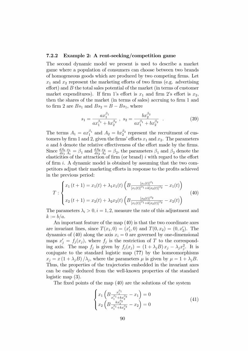
7.2.2 Example 2: A rent-seeking/competition game

The second dynamic model we present is used to describe a marketgame where a population of consumers can choose between two brandsof homogeneous goods which are produced by two competing firms. Letx1 and x2 represent the marketing efforts of two firms (e.g. advertisingeffort) andB the total sales potential of the market (in terms of customermarket expenditures). If firm 1’s effort is x1 and firm 2’s effort is x2,then the shares of the market (in terms of sales) accruing to firm 1 andto firm 2 are Bs1 and Bs2 = B −Bs1, where

s1 =ax

β11

axβ11 + bx

β22

, s2 =bx

β22

axβ11 + bx

β22

. (39)

The terms A1 = axβ11 and A2 = bx

β22 represent the recruitment of cus-

tomers by firm 1 and 2, given the firms’ efforts x1 and x2. The parametersa and b denote the relative effectiveness of the effort made by the firms.Since dA1

dx1x1A1= β1 and

dA2dx2

x2A2= β2, the parameters β1 and β2 denote the

elasticities of the attraction of firm (or brand) i with regard to the effortof firm i. A dynamic model is obtained by assuming that the two com-petitors adjust their marketing efforts in response to the profits achievedin the previous period:

T :

x1 (t+ 1) = x1(t) + λ1x1(t)

³B [x1(t)]

β1

[x1(t)]β1+k[x2(t)]

β2− x1(t)

´x2 (t+ 1) = x2(t) + λ2x2(t)

³B [x2(t)]

β2

[x1(t)]β1+k[x2(t)]

β2− x2(t)

´ (40)

The parameters λi > 0, i = 1, 2, measure the rate of this adjustment andk := b/a.An important feature of the map (40) is that the two coordinate axes

are invariant lines, since T (x1, 0) = (x01, 0) and T (0, x2) = (0, x02). The

dynamics of (40) along the axis xi = 0 are governed by one-dimensionalmaps x0j = fj(xj), where fj is the restriction of T to the correspond-ing axis. The map fj is given by fj(xj) = (1 + λjB)xj − λjx

2j . It is

conjugate to the standard logistic map (??) by the homeomorphismsxj = x (1 + λjB) /λj, where the parameters µ is given by µ = 1 + λjB.Thus, the properties of the trajectories embedded in the invariant axescan be easily deduced from the well-known properties of the standardlogistic map (3).The fixed points of the map (40) are the solutions of the system

x1³B

xβ11

xβ11 +kx

β22

− x1´= 0

x2³B

kxβ22

xβ11 +kx

β22

− x2´= 0

(41)

90

There are three evident “boundary solutions”,

O = (0, 0) ; E1 = (B, 0) ; E2 = (0, B) , (42)

but O is not a fixed point because the map is not defined in it. Thefixed points E1 and E2 are related to the positive fixed points of the one-dimensional quadratic maps f1 and f2 governing the dynamics along theinvariant axes. There is also another fixed point, interior to the positivequadrant R2+, given by

E∗ = (x∗1, B − x∗1) . (43)

The coordinate x∗1 ∈ (0, B) is the unique solution of the equation F (x) =k

11−β2 x

1−β11−β2 + x − B = 0, since F a continuous function with F (0) < 0,

F (B) > 0 and F 0(x) > 0 for each x > 0. With a given set of parametersB, β1 and β2, the positive fixed point E∗ is locally asymptotically stablefor sufficiently small values of the adjustment speeds λ1 and λ2. It losesstability as one or both of the adjustment speeds are increased and morecomplex attractors are created around it.In the following we focus our attention on the global properties of

the map (40), in particular on the boundaries of the feasible set B. Thisfeasible set is defined as the set of points which generate trajectorieswhich are entirely in the positive orthant (feasible trajectories). A feasi-ble trajectory may converge to the positive fixed point E∗, to other morecomplex attractors inside B or to a one-dimensional invariant set embed-ded inside a coordinate axis (the last occurrence means that one of thetwo brands disappears). Trajectories starting outside of the set B repre-sent infeasible evolutions of the economic system. As proved in Bischi,Gardini and Kopel [21], (40) is a noninvertible map of Z4 > Z2−Z0 type,and the qualitative shape of the critical curves, as well as the Riemannfoliation, are similar to the ones of the previous example, see Fig.64c. Asbefore, starting from the knowledge of the global properties of the map(40), we illustrate how the boundaries of the feasible set changes whena structural parameter of the game is changed. By using the method ofcritical curves, we try to reveal the mechanism which is responsible forthese changes.With values of the parameters βi in the range (0.2, 0.3), our nu-

merical investigation has shown that the invariant coordinate axes aretransversely repelling, i.e. they act as repelling sets with respect to tra-jectories approaching them from the interior of the nonnegative orthant.Moreover, for the parameters used in our simulations, we have observedonly one attractor inside B, although more than one coexisting attrac-tors may exist, each with its own basin of attraction. On the basis of

91

this numerical evidence, in what follows we will often speak of a uniquebounded and positive attracting set A, which attracts the generic fea-sible trajectory, even if its existence and uniqueness are not rigorouslyproved. Let ∂B be the boundary of B. Such a boundary can have asimple shape, as in the situation shown in Fig.67a, where the attractorA is the fixed point E∗ and B is represented by the white region. How-ever, the basin can also have a very complex structure, as in Fig.67b,where, again, B is given by the white points and A is a chaotic attractorrepresented by the black points inside B.

Fig.67

An exact determination of ∂B is the main goal of the remainder of thisanalysis. Let us first consider the dynamics of T restricted to the invari-ant axes. We know that the maps fj that govern the dynamics along theinvariant axes are topologically conjugated to the logistic map (3). Thisinsight is important, and the reader is urged to recall the properties ofthis one-dimensional map (see Section 2). For λ1B ≤ 3 (correspondingto µ ≤ 4), we can deduce that bounded trajectories along the x1 axisare obtained, as long as the initial conditions are taken inside the seg-ment ω1 = OO

(1)−1. The point O

(1)−1 is the rank-1 preimage of the origin O

computed for the one-dimensional restriction f1, i.e.

O(1)−1 =

µ1 + λ1B

λ1, 0

¶. (44)

Divergent trajectories along the x1 axis are obtained starting from aninitial condition out of the segment ω1. Analogously, when λ2B ≤ 3,bounded trajectories along the invariant x2 axis are obtained providedthat the initial conditions are taken inside the segment ω2 = OO

(2)−1. In

92

this case the point O(2)−1 is the rank-1 preimage of the origin computed

for the restriction f2, i.e.

O(2)−1 =

µ0,1 + λ2B

λ2

¶. (45)

Divergent trajectories along the x2 axis are obtained starting from aninitial condition out of the segment ω2. Consider now the region boundedby the segments ω1 and ω2 and their rank-1 preimages ω−11 = T−1 (ω1)and ω−12 = T−1 (ω2). Such preimages can be analytically computed asfollows. Let X = (p, 0) be a point of ω1, i.e. 0 < p < 1+λ1B

λ1. Its

preimages are the real solutions of the algebraic system obtained from(40) with (x01, x

02) = (p, 0):

x1³1 + λ1B

xβ11

xβ11 +kx

β22

− λ1x1´= p

x2³1 + λ2B

kxβ22

xβ11 +kx

β22

− λ2x2´= 0

(46)

It is easy to see that the preimages of the point X are either located onthe same invariant axis x2 = 0 (in the points whose coordinates are thesolutions of the equation f1(x1) = p) or on the curve of equation

x1 =

·kx

β22

µλ2B − λ2x2 + 1

λ2x2 − 1¶¸ 1

β1

. (47)

Analogously, the preimages of a point Y = (0, q) of ω2, i.e. 0 < q <1+λ2Bλ2

, belong to the same invariant axis x1 = 0 (in the points whosecoordinates are the solutions of the equation f2(x2) = q), or lie on thecurve of equation

x2 =

"xβ11

k

µλ1B − λ1x1 + 1

λ1x1 − 1¶# 1

β2

. (48)

It is straightforward to see that the curve (47) intersects the x2 axis inthe point O(2)

−1 given in (45), the curve (48) intersects the x1 axis in thepoint O(1)

−1 given in (44), and the two curves (47) and (48) intersect at apoint O(3)

−1 interior to the positive orthant (see Fig.67a). The point O(3)−1 is

another rank-1 preimage of the origin. The four preimages of the originare the vertexes of a “quadrilateral” OO(1)

−1O(3)−1O

(2)−1, whose sides are ω1,

ω2 and their rank-1 preimages ω−11 and ω−12 , which are located on thecurves of equation (47) and (48). All the points outside this quadrilateralcannot generate feasible trajectories. In fact, points located on the right

93

of ω−12 are mapped into points with negative x1 coordinate after oneiteration, as can be easily deduced from the first line of (40). Pointslocated above ω−11 are mapped into points with negative x2 coordinateafter one iteration, as can be deduced from the second line of (40).The boundary of B is given, in general, by the union of all preimages

(of any rank) of the segments ω1 and ω2:

∂B(∞) =µ ∞Sn=0

T−n (ω1)¶∪µ ∞Sn=0

T−n (ω2)¶. (49)

As long as λ1B ≤ 3 and λ2B ≤ 3 the boundary of B has the simple shapeshown in Fig.67a, because no preimages of higher rank of ω1 and ω2 exist.This is due to the fact that ω−11 and ω−12 are entirely included inside theregion Z0 of the plane whose points have no preimages. The situation isdifferent when the values of the parameters are such that some portionsof these curves belong to the regions Z2 or Z4 whose points have twoand four preimages respectively. In this case preimages of higher orderof ω1 and ω2 exist, say ω−k1 and ω−k2 , which form new portions of ∂B.Such preimages of ω1 and ω2 of rank k > 1 bound regions whose pointsare mapped out of the feasible set B after k iterations. In such a casethe shape of the boundary of B becomes far more complex. This changeis due to a global bifurcation that can be explained by using the criticalcurves.If λ1 or λ2 are increased so that the bifurcation value λb = 3/B

is crossed by at least one of them, then ∂B changes from smooth tofractal. To see this, we fix the parameters B, k, β1, β2 and λ1 andvary the speed of adjustment λ2. As λ2 is increased, the branch LC(b)

of the critical curve that separates Z0 from Z2 moves upwards, andat λ2 = 3/B it has a contact with ω−11 at the point O(2)

−1. After thiscontact, a segment of ω−11 enters the region Z2, so that a portion S1 ofthe infeasible set, bounded by LC(b) and ω−11 , now has two preimages(see Fig.67b). These two preimages, say S

(1)0 and S

(2)0 , merge in points

of LC(b)−1 (as the points of LC

(b) have two merging preimages belongingto LC

(b)−1) and form a “grey tongue” issuing from the x2 axis (denoted

by S0 in Fig.67b, with S0 = S(1)0 ∪ S(2)0 ). S0 belongs to the “grey set” of

points that generate infeasible trajectories because the points of S0 aremapped into S1, so that negative values are obtained after two iterations.Again, it is important to recall the fact that along the axes the dynamicalbehavior is governed by one-dimensional maps which are conjugate to thelogistic map. We already know that the logistic map undergoes a globalbifurcation at µ = 4, where a contact between the critical point and thebasin boundary occurs. This global bifurcation changes the structureof the basin for the one-dimensional map. A similar mechanism is at

94

work here. To see this, look at the intersection of the “main tongue”S0 with the x2 axis. This gives a set I0 around the critical point c2of the restriction f2. Of course, I0 corresponds to the “main hole inthe middle part” of the logistic map with µ > 4 (Fig.62b, or in theMyrberg’s map for b > 2, see Fig.14b). However, we already know thatI0 has an infinite sequence of further preimages, I

(1)−1 and I

(2)−1 , and so

on. Accordingly, the set S0 is only the first of infinitely many preimagesof S1. Preimages of S1 of higher rank form a sequence of smaller andsmaller grey tongues issuing from the x2 axis, whose intersection with thex2 axis correspond to the infinitely many preimages I−k of the main holeI0. Only some of them are visible in Fig.67b, but smaller tongues becomenumerically visible by enlargements, as it usually happens with fractalcurves. The fractal structure of the boundary of B is a consequence ofthe fact that the tongues are distributed along the segment ω2 of the x2axis according to the structure of the intervals I−k described in Section2, whose complementary set is a Cantor set. In the situation shown inFig.67b the main tongue S0 has a wide portion in the region Z4. Hence,besides the two preimages along the x2 axis (denoted by S

(1)−1 and S

(2)−1

in Fig.67b) issuing from the intervals I(1)−1 and I(2)−1 , two more preimages

exist. Hence, in the two-dimensional case the structure of the basin iseven more complex. The additional preimages are denoted by S

(3)−1 and

S(4)−1 in Fig.67b, and are located at opposite sides with respect to LC

(a)−1 .

The tongues S(3)−1 and S(4)−1 belong to Z0, hence they do not give rise to

new sequences of tongues. On the other hand, S(1)−1 and S(2)−1 have further

preimages, since they are located inside Z4 and Z2 respectively. If thepreimages are two, as in the case of S(2)−1 , they form two tongues issuingfrom the x2 axis. In the case of four preimages, as in the case of S

(1)−1 ,

two of them are tongues issuing from the x2 axis and two are tonguesissuing from the opposite side, i.e. ω−12 .As λ2 is further increased, LC(b) moves upwards, the portion S1

enlarges and, consequently, all its preimages (i.e. the infinitely manytongues) enlarge and become more pronounced. This causes the occur-rence of another global bifurcation, that changes the set B from simplyconnected to multiply connected (or connected with holes). The mecha-nism is similar to the one described in Mira et al. [89], [88] and Abrahamet al. [1]. This second global bifurcation occurs when a tongue, belong-ing to Z2, has a contact with LC(a) and subsequently enters the regionZ4. If such a contact occurs out of the x2 axis, it causes the creation ofa pair of new preimages. These preimages merge along LC(a)

−1 and theirunion is a hole (or lake, following the terminology introduced in Mira etal. [88]) inside the feasible set B. Accordingly, a set of points that gener-

95

ate infeasible trajectories has been created, and this set is surrounded bypoints of the feasible set B. Such a situation is shown in Fig.68a, wherea tongue has crossed LC(a) and the set H1 is now in Z4. The hole H0

of infeasible points is the preimage of the set H1, and is completely in-cluded in the feasible set. As λ2 is further increased, other tongues crossLC(a) and, hence, new holes are created, giving a complicated structureof B like the one shown in Fig.68b, where many holes inside B are clearlyvisible.

Fig.68

To sum up, the transformation of the set B from a simply connected re-gion with smooth boundaries into a multiply connected set with fractalboundaries occurs through two types of global bifurcations, both due tocontacts between ∂B and branches of the critical set LC. In Fig.68b itcan be noticed that also the attractor inside B changed its structure.For low values of λ2, as in Fig.68a, the attractor is the fixed point E∗,to which all the trajectories starting inside the set B converge. As λ2 in-creases, E∗ loses stability through a flip (or period doubling) bifurcation,at which E∗ becomes a saddle point, and an attracting cycle of period2 is created near it. As λ2 is further increased, a sequence of perioddoublings occurs, similar to the well-known Myrberg (or Feigenbaum)cascade for one-dimensional maps, which creates a sequence of attractingcycles of period 2n followed by the creation of chaotic attractors, whichmay be cyclic chaotic sets or a connected chaotic set. So, both kinds ofcomplexities can be observed in this model, even if there are no relationsbetween them (for more details see Bischi, Gardini and Kopel, [21]).

96

8 Piecewise smooth systems.

In this section we shall consider maps which are not continuously differ-entiable or not continuous. These maps may undergo bifurcations whichare not described by those already seen in the previous Sections. In fact,in such cases a new kind of bifurcation may occur, which involves thedisconitinuity point or set, which is the locus in which the discontinu-ity occurs (either in the first derivative or in the function definition).These new kind of bifurcations are nowadays known as "Border Colli-sion Bifurcations" (BCB henceforth). This kind of bifurcation is a quiterecent topic of research. We shall consider here only piecewise smoothcontinuous systems, giving some results for maps in 1D and 2D phasespaces.

8.1 1D map.A recent application in the conomic context (see Gardini, Sushko andNaimzada, 2008 [39]) may be useful to introduce the subject associatedwith a one-dimensional piecewise smooth map. Besids this work we referto [53], [59], [75], [77], [94], [95], [31], [15], [106], [107], for some worksrelated to one-dimensional piecewise smooth maps.Let us consider the model first proposed by Matsuyama in [81], which

describes the interaction of two sources of economic growth: The mech-anism of capital accumulation and the process of technical change andinnovation. Matsuyama constructed a one-dimensional dynamic modeldescribed by two different functions, each of which characterizes a differ-ent regime: The Solow regime, with high rates of growth, no innovationsand a competitive market structure, as in the neoclassical model, andthe Romer regime, with low rates of growth, innovations and a monopo-listic market structure, as in the neo-shumpeterian model. In this modelthe dynamics often alternates between the two different regimes: Thereis a trade off between growth and innovation. Analytically the model isrepresented by a piecewise smooth unimodal map, xt+1 = φ(xt), wherethe function φ(x) is given by

φ(x) =

(f(x) = Gx1−

1σ if 0 < x < 1 (Solow regime)

g(x) = Gx1+θ(x−1) if x > 1 (Romer regime)

(50)

with θ = (1− 1σ)1−σ, and σ > 1. The independent variable xt corresponds

to the independent variable kt in the original paper [81], that is, xt =Kt

NtσFθwhereKt stands for capital, Nt the number of types of intermediate

goods introduced up to time t, and F is some constant. The outputYt is related to the amount of capital Kt, and the available types ofintermediates, Ns, 0 < s < t, through a production function. The model

97

is closed assuming that a constant proportion of the output, Yt, is leftto be used as capital in the next period. When the state is xt < 1then no innovation occurs and no new intermediates are introduced, theviceversa takes place in the case xt > 1. The two parameters of themodel are G and σ. Increasing G the gross rate of growth changes, thefixed point from the Solow region (0 < x < 1) enters the Romer region(x > 1) and for σ > 2 is destabilized. The parameter σ denotes thedemand elasticity of the intermediate good (and the monopoly margin),and also has a meaning in determining the share of labor ( 1

σ).

Besides Matsuyama, the same model was also considered by Mitra in[90], Mukherjy in [91], and the complete analysis is reported in Gardiniet al. 2008, to which we refer for further details. Here we shall hererecall haw the use of the BCB is fundamental for the undestanding ofthe bifurcations occurring in the dynamics of the model.

Fig.69 The function φ(x) with the globally attracting fixed point x∗L in theSolow regime at G = 0.98, σ = 5 (a), and x∗R in the Romer regime at

G = 1.45, σ = 5 (b).

It is easy to see that for 1 < σ < ∞ we have 1 < θ < e, and this isthe range of interest: σ > 1. The function f(x) on the left side (Solowregime) is monotonic increasing, because f 0(x) = G(1 − 1

σ)x−

1σ > 0. It

has a unique fixed point x∗L = Gσ which exists (in its region of definition:x < 1) as long as G < 1, and when it exists, it is always stable, as 0 <f 0(x∗L) = (1− 1

σ) < 1. Furthermore, it is globally attracting except for the

origin. As the origin is always a repelling fixed point, we have restrictedour interval of interest to x > 0. As mentioned in the Introduction, atG = 1 a bifurcation occurs, and for G > (θ − 1) the fixed point in theRomer regime (x > 1) is globally asymptotically stable. In fact, thefunction g(x) defining the regime for x > 1 is monotonic decreasing andconvex (as g0(x) = − G(θ−1)

(1+θ(x−1))2 < 0, and g00(x) > 0) and it has a uniquefixed point x∗R = 1 + G−1

θwhich exists (in its region: x > 1) for any

98

G > 1, but it may be stable or unstable. From g0(x∗R) = −(θ−1G ) we havethat it is locally stable for G > (θ − 1), and it is easy to see that it isalso globally attracting.In .Fig.69a, we show the shape of the function φ(x) when the fixed

point x∗L is globally attracting (G < 1), while in Fig.69b, x∗R is globallyattracting (G > (θ−1)). We also see immediately that at the bifurcationvalue G = 1, when the fixed point is x∗ = 1, we have the left sidederivative of the function φ0L(1) = (1 − 1

σ) < 1 and independently on

the value of the derivative of the function on the right, this is enough toprove that the fixed point x∗ = 1 is globally attracting. In fact, any pointwith x > 1 is mapped in one iteration on the left side with x < 1 fromwhich the iterations converge (increasing monotonically) to the fixedpoint x∗ = 1. Similarly, due to the monotonicity of the functions on theright side for G > (θ − 1), with g(1) = G and g(G) = G2

1+θ(G−1) > 1,

we have that any point x ∈ (0, 1) will reach the region x > 1 in a finitenumber of iterations, and the region x > 1 is mapped into itself, withthe fixed point globally attracting.From the previous observations it follows that the interesting region

is the interval 1 < G < (θ − 1), and the dynamics of the model as Gvaries in this interval depend on the value of the other parameter σ. Atthe bifurcation value G = (θ − 1) all the points in the interval [1, G]belong to 2-cycles (stable but not asymptotically stable). In fact, thebifurcation value G = (θ − 1) is a degenerate flip bifurcation: all thepoints of the segments [1, x∗R) and (x

∗R, 1] are 2-cycles. We can show this

by using the change of variable which puts x∗R in the origin. That is, lety = x− x∗R then

HR(y) = g(y + x∗R)− x∗R =(1− θ)y

θy +G(51)

and

H2R(y) = HR

HR(y) =(1− θ)2y

y(θ(1− θ) +Gθ) +G2(52)

so that at the bifurcation value G = (θ − 1) we have H2R(y) = y. Any

i.c. with x > 0 will be mapped into the interval [1, G] in a finite numberof iterations, thus ending in a 2-cycle with both states in the Romerregime. It was also shown in [81] that for G < (θ − 1) there existsa 2-cycle, the dynamics “oscillate” between the Solow regime and theRomer regime, and the dynamics of the map in (50) always belong tothe absorbing interval [g(G), G]. Any point with i.c. x > 0 will enter thisinterval in a finite number of iterations, from which it will never escapesince φ([g(G), G]) ⊆ [g(G), G].

99

The rigorous proof of the bifurcations occurring in the map in (50) arenot easy, because of the complex analytical expressions. However, a nu-merical proof can first be given. In Fig.70 we present a two-dimensionalbifurcation diagram in the (G,σ)-parameter plane in which different graytonalities correspond to different dynamic regimes of the map (50).

Fig.70 Bifurcation diagram in the (G,σ)-parameter plane. The lightest graycolor corresponds to the parameter values at which the map φ has a stablefixed point (which is x∗L for G < 1, or x∗R for G > 1, G > (θ− 1)), followed

by a strip related to the parameter values at which the map φ has anattracting cycle of period 2, and in sequence gray tonalities correspond to

4-, 2- and 1-piece chaotic intervals, respectively.

Let us here consider the parameter values corresponding to the existenceof a two-cycle. Since in the Romer regime the function g(x) is decreas-ing and convex, we have that the first derivative g0(x) is negative and itincreases as x increases from 1 (but remaining g0(x) < 0). It follows thatif the derivative in the critical point satisfies −1 < g0(1) we must have−1 < g0(x) < 0 for any x > 1. From the expression g0(1) = −G(θ − 1)we have that |g0(1)| < 1 whenever both the conditions hold, G < 1 andθ ≤ 2, which corresponds to σ ≤ 2. Moreover, in the (G,σ)-parameterplane the bifurcation curve of equation G = (θ−1) issues from the point(G, σ) = (1, 2) and is increasing and convex - as can be seen in Fig.2(this fact was also proven in [91]). Thus, the line σ = 2 never intersectsthe bifurcation curve G = (θ− 1) (apart from the issuing point). So, allthe interesting dynamics occur at fixed values of σ with σ > 2, otherwisewe must have a stable fixed point (either on the left, if G < 1, or on the

100

right, if G > 1). It follows that in order to detect a stable 2-cycle wemust have σ > 2, which corresponds to (θ − 1) > 1. Now let us assumethat σ > 2 is fixed and G decreases, starting from some value G > (θ−1)for which x∗R is stable (see Fig.70). Then, as we have seen above, the lossof stability of x∗R occurs via a degenerate bifurcation: At the bifurcationvalue G = (θ − 1) all the points of a segment are 2-cycles. In particular1, G forms a 2-cycle. After the bifurcation, for G < (θ − 1), the fixedpoint x∗R is unstable. Furthermore no stable 2-cycle can exist with boththe points on the right, in the Romer regime. This is proved by thefact that we have g0(x) < −1 for all the points x in the interval [1, G],because in the iterated map HR HR(y) we have the slope equal to 1 inall the points of a segment (see Fig.71a where φ(x) and φ2(x) are shownat the bifurcation value G = (θ − 1)), while after the bifurcation (seeFig.71b, where G < (θ − 1)) we have the slope greater than 1 in thesegment x ∈ [1, G].

Fig.71 The functions φ(x) and φ2(x) at the critical flip bifurcation valueG = (θ − 1) = 1.441408, σ = 5 (a) and after, at G = 1.4 < (θ − 1) (b).This is rigorously proved by using

d

dyH2

R(y) =(1− θ)2G2

[y(θ(1− θ) +Gθ) +G2]2=

(1−θG)2

[y(θ(1−θ)+Gθ)G2

+ 1]2

from which we have ddyH2

R(0) > 1. Moreover, from (θ − 1) > G, wehave θ(θ − 1) > Gθ so that Gθ + θ(1 − θ) < 0, and for y in a rightneighborhood of 0 the denominator of d

dyH2

R(y) is less than 1, and thusddyH2

R(y) > (1−θG)2 > 1. From the considerations given above, it follows

that a unique 2-cycle exists after the bifurcation, forG < (θ−1), with onepoint of the cycle in the Solow regime and one point in the Romer regime,xL, xR. From stable (inside the wide region) it becomes unstable as

101

G decreases reaching the value G = G4 in Fig.70. The local stability ofthis unique 2-cycle was already studied in [91], and a sufficient conditionfor its stability is given, depending on the points of the 2-cycle:

|φ0(xL)φ0(xR)| =x1σL (1− 1

σ)(θ − 1)

G2< 1. (53)

The bifurcation occurs when |φ0(xL)φ0(xR)| = 1 in (53), once that theexplicit expression of xL is there inserted, but this is not known, thusit is difficult to obtain an explicit form. However, a different way toget the bifurcation condition comes from considering the images of thecritical point x = 1 (or equivalently of its first iterate x = G). It canbe noticed that the bifurcation occurring at G = (θ − 1) increasing G,for the existing stable 2-cycle (with points xL < 1 < xR) correspondsto a border-collision bifurcation: The periodic point xL merges with thecritical point x = 1, which is a 2-cycle at this parameter value. The con-dition G = (θ − 1) may thus be written also as φ(G) = 1 or φ2(1) = 1,which reads explicitly also as g2(1) = 1. Similarly, at the bifurcationin which the stable 2-cycle becomes unstable as G decreases, one mightthink that a stable 4−cycle would appear. Let us first describe whatoccurs via an example.

Fig.72 The functions φ(x) and φ4(x) at the parameter values G = 1.1,σ = 5 in (a) and G = 1.073, σ = 5 in (b), for which the map φ has the

attracting 2-cycle.

In Fig.72a (G = 1.1), we show the same example considered by Mukherji(σ = 5) at a value of G in which the 2-cycle is stable. We can see thatthis corresponds to two stable fixed points for the iterated map φ2(x).It can be also seen that the bifurcation structure is quite similar to thecritical situation occurring at the bifurcation of the fixed point. That is,as G decreases approaching the bifurcation value, in the graph of φ4(x)

102

two segments tend to collide with the diagonal. In fact this can clearly beseen in Fig.72b (G = 1.073), although the parameters are only close tothe bifurcation value and the iterations of the critical point still tend tothe stable 2-cycle. The bifurcation occurs at approximately G = 1.0725,as shown in Fig.73a, where we have indeed that the points 1, G, g(G),and f g(G) form a 4-cycle, and the points of the segments [g(G), 1],[fg(G), G] are all fixed points for the map φ4(x) (corresponding to all4-cycles for φ and only one 2-cycle with periodic points approximatelyin the center of the two intervals). It can be noticed that at the bifurca-tion value, | d

dxφ4(x)|≥ 1 for all the points of the absorbing segment of the

map, thus it is impossible to get a stable 4-cycle after the bifurcation. Infact, after the bifurcation (see Fig.73b), also the segments previously onthe diagonal now have slopes higher than 1, thus we have | d

dxφ4(x)|> 1

in all the points of the absorbing interval.

Fig.73 The functions φ(x) and φ4(x) at the parameter values G = 1.0725,σ = 5, are related approximately to the critical flip bifurcation of the

2-cycle in (a) and after the bifurcation, at G = 1.05, σ = 5, when the mapφ has 4-cyclical chaotic intervals in (b).

It turns out that a stable 4-cycle is impossible. Moreover, any cycle ofany period cannot be stable, because φ4 is expanding in the absorbinginterval [g(G), G]. Instead, all the asymptotic trajectory inside this in-terval tend to the unique attractor, which is chaotic and made up of 4cyclical chaotic intervals for the map φ (corresponding to four invariantchaotic intervals for φ4), which are bounded by the images of the criticalpoint, that is: φi(1) for i = 1, 2, ..., 8 (i.e., G, g(G), ...). The consid-erations given above also show that the bifurcation condition in (53) isequivalent to the condition φ4(1) = 1 (the critical point must be periodicof period four), which is given by

g f g2(1) = 1. (54)

103

We can so state the following:

Proposition. The stability region of the 2-cycle of the map in (50),shown in Fig.70, for any fixed value σ > 2, is bounded by the curves ofimplicit equations g2(1) = 1 (which corresponds explicitly to G = (θ−1))and g f g2(1) = 1 (implicit equation for G(σ) = G4).

The critical bifurcation of the 2-cycle (related with its stability/ in-stability) also corresponds to the bifurcation curve at which the 4 pieceschaotic intervals undergo a border collision bifurcation, and thus thecondition is obtained either from φ4(1) = 1 which corresponds to thecondition given in (54), or from the equality in (53) (but there, the co-ordinate of the point xL of the 2-cycle is not analytically known). Wehave seen numerically that for any fixed value of σ > σ4 (' 3.825) theequation given in (54) has a single solution, which we have called G4 inthe Proposition.

8.1.1 Chaotic intervals

Really the proof given in the previous subsection of the dynamics ofthe map is numerical, but the slopes of the function φ4 in the absorb-ing interval are easy to see (as the pieces of the function look almostpiecewise linear, and it is enough to compare the slopes with the twodiagonals). So we state that also the bifurcation occurring for the at-tracting 2-cycle is critical (as it is proved for the fixed point), and nostable cycle can exist. Moreover, as it is easy to see numerically that ,the slopes become steepest as G further decreases towards 1, so the con-dition | d

dxφ4(x)| > 1 persists at any lower value of G up to 1. Thus no

period-doubling bifurcation occurs at the 2-cycle as G decreases, cross-ing through the value G = G4, at which the equation g f g2(1) = 1, orequivalently g f g(G) = 1, holds, while chaotic regimes exist. Indeed,as we see in Fig.70, it is also correct to say that cycles of period threecannot exist, but the chaotic regimes exist anyhow. As we have alreadyseen in Sections 2 and 3 it is enough to have homoclinic trajectories fora fixed point or cycle to have also chaotic dynamics. And in this specificcase the chaotic set is also of full measure. In fact, considering the fixedpoint, when the condition φ3(1) = x∗R is satisfied we have that the mapis chaotic in the whole interval [g(G), G]. It is worth noticing that thecondition given in Sections 2 and 3 says nothing about the density ofthe chaotic set Λ. Indeed, Λ may also be a set of points of zero measurein I, and in such a case the chaotic dynamics, although existing, is notdetectable by numeric simulations of a generic trajectory. The situationis different when the chaotic set is an interval or cyclical chaotic intervals(as it occurs, for example, exactly at the homoclinic bifurcation value ofa cycle). The appearance of such full measure chaotic intervals is indeed

104

what occurs in our model (50) whenever the fixed point and the 2-cycleare not stable, as stated in the followingProposition. For any fixed value σ > 2 when the fixed point and the

2-cycle of the map in (50) are unstable, the attractors are full measurechaotic intervals.In fact, the dynamics which may occur as G is further decreased

below the value G = G4 are always chaotic: After the 2-cycle, 4-cyclicalchaotic intervals appear, which may merge (say at G = G2) into 2-cyclical chaotic intervals, which in turn may merge (say at G = G1) intoone chaotic interval (see Fig.70).The bifurcation curve at which 4-cyclical chaotic intervals merge in

pairs into 2-pieces chaotic intervals (and vice-versa) is the first homo-clinic bifurcation of the repelling 2-cycle (which was external to the fourchaotic intervals). Thus this bifurcation occurs when φ6(1) = (φ2)3(1) =xL in the Solow regime or, equivalently, when the fifth iterate of the pointof maximum (x = 1) merges into the periodic point xR in the Romerregime, φ5(1) = xR, which corresponds to

g2 f g2(1) = xR. (55)

Although it is quite complicated to find it in explicit form analytically,we have numerically seen that for any fixed value of σ > σ2 (' 6.123)the equation given in (55) has a single solution, which we call G2.The 2-cyclical chaotic intervals are always bounded by the images

of the critical point (now φi(1) for i = 1, 2, 3, 4 i.e., G, g(G), ..., that is[g(G), g f g(G)], [f g(G), G]). However this does not occur at thelow value of σ (as σ = 5 in the above example). Indeed the chaoticregime may not be reached either, as can be seen also from Fig.70. Thedynamic behaviors of the map as G decreases or increases depend on thevalue of σ, for 2 < σ < σ4 we can only have a stable 2-cycle and chaoticintervals never occur at any value of G, while chaotic intervals occur forany σ > σ4.To illustrate the dynamic behavior let us show a few figures of one-

dimensional bifurcation diagrams (or orbit diagrams) at fixed values ofσ. Fig.s 74-75 show the asymptotic behavior of the state variable x (inthe vertical axis) as a function of G (in the horizontal axis). As alreadyremarked, it is worth noticing that whichever is the value of σ, as it iseasy to see from the analytical expression of g(G), as G tends to 1 g(G)also tends to 1, so that the whole absorbing interval [g(G), G] shrinksto one point, the point of maximum x = 1 and also maximum valueG = 1 (and attracting fixed point). Each figure represents the dynamicsoccurring at a crossection of the bifurcation diagram in Fig.70, at fixedvalues of σ (the crossections are indicated in Fig.70 by the straight lines

105

with arrows).

Fig.74 One-dimensional bifurcation diagrams of the map φ. σ = 3,g ∈ [0.95, 1.3] , in (a); σ = 5, g ∈ [0.95, 1.1] , in (b).

Fig.75 One-dimensional bifurcation diagrams of the map φ. σ = 15,g ∈ [0.95, 1.2] , in (a); σ = 30, g ∈ [0.95, 1.8] , in (b).

The bifurcation curves represented there, separating the different kindsof chaotic intervals, have been done numerically, by using the analyti-cal conditions related with the homoclinic bifurcations of the relevantcycles. One is the equation given in (55), while the bifurcation curve atwhich 2 pieces chaotic intervals merge into a single one (or vice-versa achaotic interval splits into two cyclical chaotic intervals) occurs when thefixed point in the Romer regime becomes homoclinic. So the condition isobtained when the third iterate of the point of maximum (x = 1) mergesinto the fixed point, φ3(1) = x∗R, which in our case corresponds to

f g2(1) = x∗R (56)

106

i.e. f g(G) = x∗R, and more explicitly reads as follows:

G

µG2

1 + θ(G− 1)¶(1− 1

σ )= 1 +

G− 1θ

. (57)

We have seen numerically that for any fixed value of σ > σ1 (' 21.231)the equation given in (57) has a single solution, which we call G1 (forexample, at σ = 50, value used by Mitra, we have G1 = 1.024254692,at σ = 22, value used by Mukherji, we have G1 = 1.001468146, atσ = 30, value used in the bifurcation diagram in Fig.75b we have G1 =1.0123131).

8.1.2 Border-collision bifurcation at G = 1

We have seen before that the bifurcations occurring at the fixed pointand the 2-cycle, which are critical bifurcations, may also be consideredas border-collision bifurcations. In fact, the bifurcation of the fixed pointoccurring for any value of σ > 2 at G = (θ − 1), may be characterizedas φ2(1) = 1, and the critical bifurcation of the 2-cycle (related with itsstability/instability) also corresponds to the bifurcation curve at which4 pieces chaotic intervals undergo a border collision bifurcation, andthus the condition is φ4(1) = 1. However, the main role of the border-collision bifurcation is clearly the one observed in the model when, at afixed values of σ, the parameter G is increased and the stable fixed pointin the Solow regime merges the point x = 1. The kinds of dynamics thatwill be observed after the border-collision bifurcation occurring at G = 1comes from the followingTheorem. The border-collision bifurcation of the fixed point x∗ = 1

of the map φ given in (50), occurring at G = 1 for any σ > 1, gives rise(as G incraeses) to• an attracting fixed point x∗R if 1 < σ < 2;• an attracting cycle of period 2 if 2 < σ < σ4 ' 3.825;• attracting 4-cyclical chaotic intervals if σ4 < σ < σ2 ' 6.123;• attracting 2-cyclical chaotic intervals if σ2 < σ < σ1 ' 21.231;• an attracting chaotic interval if σ > σ1.

Proof. The theorem can be proved by using the normal form ofthe border-collision bifurcation occurring in one-dimensional piecewisesmooth maps first proposed in [95]. According to Theorem 3 statedin [95] applied to the map φ given in (50), the result of the border-collision bifurcation of the fixed point depends on the left and right sidederivatives of φ(x) evaluated at x = 1 for G = 1, here denoted α and β,respectively:

α = limx→1−

d

dxφ(x), β = lim

x→1+d

dxφ(x). (58)

107

The related normal form is given by the skew-tent map ψ : y 7→ ψ(y)defined by the function

ψ(y) =

½αy + ε, y ≤ 0,βy + ε, y ≥ 0. (59)

Here ε is a bifurcation parameter such that as ε varies through 0, thelocal bifurcations of the piecewise linear map ψ and the piecewise smoothmap φ are of the same kind. That is, the border-collision bifurcationoccurring for the fixed point x∗ = 1 of the map φ at G = 1 is of thesame kind as the border-collision bifurcation of the fixed point y∗ = 0 ofthe map ψ occurring at ε = 0.The dynamics of the piecewise linear map ψ have already been stud-

ied (see [75], [95], [15] and references therein), and depend on the slopesα and β of the linear functions. All the possible kinds of border-collisionbifurcation of the fixed point x∗ are classified according to the parti-tion of the (α, β)-parameter plane into subregions in which the samequalitative dynamics take place.We summarize these results in Fig.76, which schematically shows the

related one-dimensional bifurcation diagrams for the border-collision ofthe fixed point of the map ψ. The cases 0 < α < 1, β < −1, and α < −1,0 < β < 1 (see the dashed regions in Fig.76), have been studied by manyauthors. They are qualitatively the same case due to the symmetry ofthe (α, β)-parameter plane with respect to the line α = β. It has beenshown that for ε > 0 (ε < 0, respectively), all trajectories are boundedand the map ψ can have an attracting cycle of any period k ≥ 2, denotedqk, as well as a cyclic chaotic interval of any period m ≥ 1, denoted Qm.This means that varying ε through 0 from ε < 0 to ε > 0 (from ε > 0to ε < 0, respectively) we can have the border-collision bifurcation fromthe attracting fixed point x∗ to any one of such attractors. The regionα > 1, α/(1− α) < β < −1 (and α < −1, 1 < β < α/(α+ 1)) includessubregions corresponding to the transition from no attractor to cyclicchaotic intervals Qm of period m = 2k, k = 0, ..., l, where l → ∞ as(α, β)→ (1,−1) ((α, β)→ (−1, 1), respectively).Now we write the coefficients of the normal form (59) in terms of the

parameter σ. From (58) we get

α =

µ1− 1

σ

¶, β = (1− θ) (60)

so that we have 0 < α < 1 and β < 0. Moreover, from 1 < θ < e wehave that 1− e < β < 0. Thus, the region of our interest in the (α, β)-parameter plane is 0 < α < 1, 1− e < β < 0 (see the thick rectangle inFig.76).

108

Fig.76

The partition of the (α, β)-parameter plane into the regions with qualitativelysimilar dynamics of the map ψ at ε < 0 (for β > α) and at ε > 0 (for β < a).Corresponding BCB of the fixed point of ψ, occuring at ε = 0 as ε variesfrom ε < 0 to ε > 0, are shown schematically by means of one-dimensionalbifurcation diagrams (the same kinds of BCB occur for α < β as ε variesfrom ε > 0 to ε < 0): The thick and dashed lines indicate attracting andrepelling cycles, respectively. The thin lines correspond to the border point.

Fig.77

The enlarged window of Fig.76 where the BCB curve B of the fixed pointx∗ = 1 of the map φ is shown, as well as the critical flip bifurcation curve Sof the 2-cycle of the map ψ, the homoclinic bifurcation curves Hi, i = 1, 2, 4of the corresponding cycles of ψ and the bifurcation curves related to the3-cycle of ψ.

109

Substituting first θ = (1− 1σ)1−σ and then σ = 1/(1−α) into (60) we

get the expression of the border-collision curve of the fixed point x∗ = 1in terms of the parameters α and β, which is denoted as B,

B : β = 1− αα/(α−1). (61)

Fig.77 presents an enlargment of the rectangle of interest in Fig.76, andin it the curve B is shown. By using the analytic expressions of thebifurcation curves as given in [75], we can describe the regions of the(α, β)-parameter plane which are crossed by the curve B. We can seethat B intersects:1) the straight line β = −1 at a point P which is (α, β) = (0.5,−1),

related to the (critical) flip bifurcation of the fixed point y∗;2) the curve, denoted as S, given by

S : β = − 1α,

related to the (critical) flip bifurcation of the 2-cycle (after which thecurve B enter a region of 4-cyclical chaotic intervals). The intersectionpoint is denoted by α4, i.e., B ∩ S = α4;3) the curve, denoted as H2, given by

H2 : α =−1−

p1 + 4β4

2β3,

which is related to the homoclinic bifurcation of the 2-cycle of the map ψgiving rise to the transition from 4-cyclical chaotic intervals to 2-cyclicalchaotic intervals, B ∩H2 = α2;4) the curve denoted as H1 given by

H1 : β =−1 +√1 + 4α2

2α,

which is related to the homoclinic bifurcation of the fixed point y∗ of themap ψ, giving rise to the transition from 2-cyclical chaotic intervals toone chaotic interval; B ∩H1 = α1.Other bifurcation curves are also shown in Fig.77, not intersected

by B. For example the curve H4 corresponding to the transition from4-cyclical chaotic intervals to 8-cyclical chaotic intervals for the map ψ.Indeed, as proved in [75], the point (α, β) = (1,−1) is an accumulationpoint for the curves related to the transition from 2i−1-cyclical chaoticintervals to 2i-cyclical chaotic intervals, i = 2, .... The bifurcation curvesrelated to the existence and stability of a cycle of period 3 can also beseen, and it is not intersected by the curve B (which is of interest to

110

us). The “end point” for the curve B for our map is (α, β) = (1, 1− e)corresponding to the parameter value σ =∞ (or θ = e).It is clear that the curve B corresponds to the vertical line atG = 1 in

the bifurcation diagram in the (G, σ)-parameter plane shown in Fig.70,and the intersection points there evidenced: The point P corresponds toσ = 2 and the point αi corresponds to σi, for i = 4, 2, 1.To end our considerations we only have to get the approximate values

of the coordinates of the intersection points αi, i = 4, 2, 1 by using theanalytical expressions of the bifurcation curves and, via (60), to get thecorresponding values of the parameter σ. We obtain that σ4 ' 3.825,σ2 ' 6.1226 and σ1 ' 21.231.We have thus proved that the, as G increases through 1, the border-

collision bifurcation of the fixed point x∗ = 1 can directly lead to achaotic interval (for σ > σ1), as in the example shown in Fig.76b, or to2-cyclical chaotic intervals (for σ2 < σ < σ1), as in the example shownin Fig.76a, or to 4-cyclical chaotic intervals (for σ4 < σ < σ2), as in theexample shown in Fig.75b, or to a stable 2-cycle (for 2 < σ < σ4), as inthe example shown in Fig.75a.

8.2 2D Business Cycle map.As a relevant application in the economic context let us recall here theclassical works on the business cycle. As well known (we refer to [97]for details), Hicks (1950 [58]) modified the Samuelson (1939 [102]) linearmultiplier-accelerator model through introducing two constraints. Thelinear multiplier-accelerator model itself only has two options: Expo-nentially explosive or damped motion. According to Hicks, only theexplosive case is interesting, as only this produces persistent motion en-dogenously, but it had to be limited through two (linear) constraints forwhich Hicks gave factual explanations.When the cycle is in its depression phase it may happen that income

decreases so fast that more capital can be dispensed with than whatdisappears through depreciation, i.e., natural wear and aging. As aresult, the linear accelerator would predict not only negative investments(disinvestments), but to an extent that implies active destruction ofcapital. To avoid this, Hicks introduced his floor to disinvestment at thenatural depreciation level.When the cycle is in its prosperity phase, then it may happen that

income would grow at a pace which does not fit available resources. Hickshas a discussion about what then happens, in terms of inflation, but hecontended himself with stating that (real) income could not grow fasterthan available resources which put a ceiling on the income variable.Hicks never formulated his final model with floor and ceiling math-

111

ematically, it seems that this was eventually done by Rau (1974 [100]),where the accelerator-generated investments were limited downwardsthrough the natural depreciation floor, and where the income is limitedupwards through the ceiling, determined by available resources. For-mally:

It = max(a(Yt−1 − Yt−2),−If);Ct = cYt−1;

Yt = min(Ct + It, Yc).

Eliminating Ct and It, one has the single recurrence equation:

Yt = min(cYt−1 +max(a(Yt−1 − Yt−2),−If), Y c). (62)

It remains to say that Hicks’s original discussion included an exponentialgrowth in autonomous expenditures, combined with the bounds If andY c growing at the same pace, but taking the bounds as constant anddeleting the autonomous expenditures, gives a more clear-cut version. Itwas this that was originally analyzed in detail by Hommes (1991 [59]).However, the full understanding of the bifurcation mechanisms occur-ring in that two-dimensional piecewise linear model is a recent result(see [37], [97], [109]), and mainly due to a particular degeneracy existingin that model. In fact, for the BCB occurring in the generic 2D contin-uous piecewise linear map, as we shall recall below, only recent studieshave been published up to now, and the study is very far from beingcompleted. And such studies are basic tools for the more general caseof piecewise smooth continuous maps: some examples may be found in[112], [111], [98], [99], [113]

Description of the Business Cycle mapLet xt := Yt, yt := Yt−1, d := If and r := Y c. Then the model given in(62) can be rewritten as a two-dimensional piecewise linear continuousmap F : R2 → R2 :

F :

µxy

¶7→µmin(cx+max(a(x− y),−d), r)x

¶, (63)

which depends on four real parameters: a > 0, 0 < c < 1, d > 0, r > 0.The map F is given by three linear maps Fi, i = 1, 2, 3, defined,

respectively, in three regions Ri of the phase plane:

F1 :

µxy

¶7→µ(c+ a)x− ayx

¶; (64)

R1= (x, y) : (1 + c/a)x− r/a ≤ y ≤ x+ d/a ;

112

F2 :

µxy

¶7→µ

cx− dx

¶; (65)

R2= (x, y) : y > x+ d/a, x ≤ (d+ r)/c ;

F3 :

µxy

¶7→µ

rx

¶; (66)

R3=R2/R1/R2.

Three half lines denoted LC−1, LC 0−1 and LC 00

−1 are boundaries of theregions Ri:

LC−1 : y = x+ d/a, x ≤ (r + d)/c,

LC 0−1 : y = (1 + c/a)x− r/a, x < (r + d)/c,

LC 00−1 :x = (r + d)/c, y > (r + d)/c+ d/a.

Their images by F are called critical lines:

LC0 : y = (x+ d)/c, x ≤ r,

LC 00 :x = r, y < (r + d)/c.

The image of LC 00−1 by F is a point (r, (r + d)/c). A qualitative view of

the phase plane of the map F for a > 1, d < r and a > c2/(1 − c) isshown in Fig.78 (the last inequality indicates that the intersection pointof LC 0

−1 and LC0 is in the negative quadrant).

Fig.78 Critical lines of the map F for a > 1, d < r, a > c2/(1− c).

113

As mentioned above, an analogous model has been studied by Hommesin [59], and the main conclusions there given hold also for the map F ,namely, for a > 1 the map F has an attracting set C homeomorphicto a circle and all the trajectories of F (except for the fixed point) areattracted to this set. It was also proved that the dynamics of the map Fon C are either periodic or quasiperiodic. We show how the set C appearsrelated to the center bifurcation of the fixed point, showing the structureof the two-dimensional bifurcation diagram in the (a, c)-parameter plane.First note that the maps F2 and F3 have simple dynamics: The

eigenvalues of F2 are µ1 = c, 0 < c < 1, µ2 = 0, so that any ini-tial point (x0, y0) ∈ R2 is mapped into a point of LC0, while the mapF3 has two zero eigenvalues, and any (x0, y0) ∈ R3 is mapped intoa point of the straight line x = r. In such a way the whole phaseplane is mapped in one step to the straight line x = r and a coneD = (x, y) : y ≤ (x+ d)/c, x ≤ r (see Fig.78). Thus, the map F is anoninvertible map of so-called (Z∞−Z1−Z0) type: Any point belongingto the critical lines or to the half line x = r, y > (r+ d)/c, has infinitelymany preimages, any inner point of D has one preimage and any otherpoint of the plane has no preimages.The map F has a unique fixed point (x∗, y∗) = (0, 0) which is the

fixed point of the map F1 (while the fixed points of the maps F2 andF3 belong to R1, thus, they are not fixed points for the map F ). Theeigenvalues of the Jacobian matrix of F1 are

λ1,2 = (a+ c±p(a+ c)2 − 4a)/2, (67)

so that for the parameter range considered the fixed point (x∗, y∗) is anode if (c + a)2 > 4a, and a focus if (c + a)2 < 4a, being attracting fora < 1 and repelling for a > 1. Thus, for a < 1 the fixed point (x∗, y∗)is the unique global attractor of the map F (given that F2 and F3 arecontractions).

Center bifurcation (a = 1)At a = 1 the fixed point (x∗, y∗) loses stability with a pair of complex-conjugate eigenvalues crossing the unit circle, that is the center bifurca-tion occurs. First we describe the phase portrait of the map F exactlyat the bifurcation value a = 1. Analogous description is presented inSection 2.2 of Chapter 2 for a two-dimensional piecewise linear map de-fined by two linear maps, which for the particular parameter value b = 0are the maps F1 and F2 given in (64) and (65). It is proved that for theparameter values corresponding to the center bifurcation there exists aninvariant region in the phase plane, which either is a polygon boundedby a finite number of images of a proper segment of the critical line,or the invariant region is bounded by an ellipse and all the images of

114

the critical line are tangent to this ellipse (see Propositions 1 and 2 ofChapter 2). In the following we use these results for the considered mapF specifying which critical lines are involved in the construction of theinvariant region.The map F1 at a = 1 is defined by a rotation matrix. Moreover, if

c = cm/ndef= 2 cos(2πm/n)− 1, (68)

then the fixed point (x∗, y∗) is locally a center with rotation numberm/n, so that any point in some neighborhood of (x∗, y∗) is periodicwith rotation number m/n, and all points of the same periodic orbit arelocated on an invariant ellipse of the map F1. Note that from c > 0 itfollows that m/n < 1/6. Denote

c = c∗def= 1− (d/r)2. (69)

Proposition. Let a = 1, c = cm/n, then in the phase space of themap F there exists an invariant polygon P such that

• if cm/n < c∗ then P has n edges which are the generating segmentS1 ⊂ LC−1 and its n − 1 images Si+1 = F1(Si) ⊂ LCi−1, i =1, ..., n− 1;

• if cm/n > c∗ then P has n edges which are the generating segmentS01 ⊂ LC 0

−1 and its n− 1 images S0i+1 = F1(S0i) ⊂ LC 0

i−1;

• if cm/n = c∗ then P has 2n edges which are the segments Si andS0i, i = 1, ..., n.

Any initial point (x0, y0) ∈ P is periodic with rotation number m/n,while any (x0, y0) /∈ P is mapped in a finite number of steps into theboundary of P.

The value c∗ is obtained from the condition of an invariant ellipseof F1 to be tangent to both critical lines LC−1 and LC 0

−1. It can beshown that for cm/n < c∗ only the upper boundary LC−1 is involved inthe construction of the invariant region, while if cm/n > c∗ we have toiterate the generating segment of the lower boundary LC 0

−1 to get theboundary of the invariant region.An example of the invariant polygon P in the case cm/n = c∗ is

presented in Fig.79, where a = 1, d = 10, r = 10/p2−√2, c = c1/8 =

c∗ =√2 − 1. For such parameter values the polygon P has 16 edges,

which are the segments Si ⊂ LCi−2 and S0i ⊂ LC 0i−2, i = 1, ..., 8. Any

point of P is periodic with rotation number 1/8 (in Fig.79 the points of

115

two such cycles belonging to the boundary of P are shown by black andgray circles), while any point (x0, y0) /∈ P is mapped to the boundary ofP .

Fig.79 The invariant polygon P with 16 edges at a = 1,

c = c1/8 =√2− 1 = c∗, d = 10, r = 10/

p2−√2.

Consider now the case in which the map F1 is defined by the rotationmatrix with an irrational rotation number ρ, which holds if

c = cρdef= 2 cos(2πρ)− 1, (70)

where ρ < 1/6. Then any point in some neighborhood of the fixed point(x∗, y∗) is quasiperiodic, and all points of the same quasiperiodic orbitare dense on the corresponding invariant ellipse of the map F1. Usingthe values c∗ given in (69) we can state the following

Proposition. Let a = 1, c = cρ. Then in the phase space of the mapF there exists an invariant region Q, bounded by an invariant ellipse Eof the map F1 which is tangent to LC−1 (and to all its images) if c < c∗,to LC 0

−1 if c > c∗, and to both critical lines LC−1 and LC 0−1 if c = c∗.

Any initial point (x0, y0) ∈ Q belongs to a quasiperiodic orbit dense in thecorresponding invariant ellipse of F1, while any initial point (x0, y0) /∈ Qis mapped to E.Note that from (69) it follows that if d > r then the inequality c∗ < 0holds, thus, given c > 0, for d > r only the lower boundary LC 0

−1 is in-volved in the construction of the invariant region of the map F at a = 1.

Bifurcation structure of the (a, c)-parameter plane

116

We describe now the dynamics of the map F after the center bifurca-tion, that is for a > 1. In short, an initial point (x0, y0) from someneighborhood of the unstable fixed point (x∗, y∗) moves away from itunder the map F1 and in a finite number k of iterations it necessar-ily enters either the region R2, or R3 (in the case in which (x∗, y∗) isa focus the statement is obvious, while if (x∗, y∗) is a repelling nodethis can be easy verified using the eigenvalues λ1,2 given in (67) andthe corresponding eigenvectors). If (xk, yk) ∈ R2, then the map F2 isapplied: F2(xk, yk) = (xk+1, yk+1) ∈ LC0. All consequent iterationsby F2 give points on LC0 approaching the attracting fixed point of F2(which belongs to R1), until the trajectory enters R1 where the mapF1 is applied again. If (xk, yk) ∈ R3, then the map F3 is applied:F3(xk, yk) = (xk+1, yk+1) ∈ LC 0

0. We have that either (xk+1, yk+1) ∈ R1,or (xk+1, yk+1) ∈ R3 and one more application of F3 gives its fixed point(r, r) ∈ R1, so, the map F1 is applied to this point. In such a way thedynamics appear to be bounded.Indeed, it was proved in Hommes [59], that for a > 1 any trajectory

of F rotates with the same rotation number around the unstable fixedpoint, and it is attracted to a closed invariant curve C homeomorphic toa circle. It was also proved that the dynamics of F on C, depending onthe parameters, are either periodic or quasiperiodic. We can state thatsuch a curve C is born due to the center bifurcation of the fixed point,described in the previous section: Namely, the bounded region P (or Q),which is invariant for a = 1, exists also for a > 1, but only its boundaryremains invariant, and this boundary is the curve C.In the subsection below we shown that also in a more generic case of

a two-dimensional piecewise linear map, defined by two linear maps, thecenter bifurcation can give rise to the appearance of a closed invariantattracting curve C, on which the map is reduced to a rotation with ra-tional or irrational rotation number. Recall that in the case of a rationalrotation number m/n the map has an attracting and a saddle m/n-cycleon C, so that the curve C is formed by the unstable set of the saddlecycle, approaching the points of the attracting cycle. While in the caseof an irrational rotation number the map has quasiperiodic orbits on C.In Section 2.3 of Chapter 2 the curve C is described in detail for the mapdefined by the linear maps F1 and F2 given in (64) and (65). So, we canuse these results for the considered map F if the curve C belongs to theregions R1, R2 and has no intersection with the region R3, thus, only themaps F1 and F2 are involved in the asymptotic dynamics. Obviously,we have a qualitatively similar case if the curve C has no intersectionwith the region R2 and, thus, only the maps F1 and F3 are applied tothe points on C. One more possibility is the case in which the curve

117

C belongs to all the three regions Ri, i = 1, 2, 3. We can state that inthe first and second cases the curve C can be obtained by iterating thegenerating segment of LC−1 and LC 0

−1, respectively, while in the thirdcase both generating segments can be used to get the curve C.

Fig.80 Two-dimensional bifurcation diagram of the map F in the(a, c)-parameter plane at d = 10, r = 30. Regions corresponding toattracting cycles of different periods n ≤ 41 are shown by various gray

tonalities.

To see which parameter values correspond to the cases described abovewe present in Fig.80 a two-dimensional bifurcation diagram in the (a, c)-parameter plane for fixed values d = 10, r = 30. Different gray tonalitiesindicate regions corresponding to attracting cycles of different periodsn ≤ 41 (note that regions related to the attracting cycles of the sameperiod n, but with different rotation numbers are shown by the samegray tonality). The white region in Fig.80 is related either to periodicorbits of period n > 41, or to quasiperiodic orbits. Let us first commenton some particular parameter values of the bifurcation line a = 1. Asdescribed in the previous section, at a = 1, c = cm/n given in (68), inthe phase plane of F there exists an invariant polygon P such that anypoint of P is periodic with the rotation number m/n. So, the pointsa = 1, c = cm/n, for different m/n < 1/6, are starting points for the cor-responding periodicity tongues. For example, a = 1, c = c1/8 =

√2− 1

is the point from which the 8-periodicity tongue starts, corresponding tothe attracting cycle with the rotation number 1/8. Recall that accordingto the summation rule (see Hao and Zheng, 1998 [55]), between any tworotation numbers m1/n1 and m2/n2 there is also the rotation numberm0/n0 = (m1 +m2)/(n1 + n2), so that a = 1, c = cm0/n0 is the starting

118

point for the corresponding periodicity region. If the (a, c)-parameterpoint is taken inside the periodicity region, then the map F has theattracting and saddle cycles with corresponding rotation number, andthe unstable set of the saddle cycle form the closed invariant attractingcurve C. Note, that in the case in which both constrains are involvedin the asymptotic dynamics, the map F may have two attracting cyclesand two saddles of the same period coexisting on the invariant curve(as it occurs, for example, inside the 7-periodicity tongue at a = 2.9,c = 0.136, d = 10, r = 30). While if the (a, c)-parameter point belongsto the boundary of the periodicity region, then the border-collision bi-furcation occurs (see [95]) for the attracting and saddle cycles, givingrise to their merging and disappearance.The parameter points a = 1, c = cρ given in (70), for different

irrational numbers ρ < 1/6 correspond to the case in which any pointof the invariant region Q is quasiperiodic. Such parameter points arestarting points for the curves related to quasiperiodic orbits of the mapF .At a = 1, c = c∗ = 8/9, (which is the value c∗ given in (69) at

d = 10 and r = 30) there exists an invariant ellipse of F1 tangent toboth critical lines LC−1 and LC 0

−1, so that for c < c∗ the boundary ofthe invariant region can be obtained by iterating the generating segmentof LC−1, while for c > c∗ we can iterate the segment of LC 0

−1. Thus,after the center bifurcation for c < c∗ at first only LC−1 is involved inthe asymptotic dynamics, and then increasing a there is a contact ofthe curve C with the lower boundary LC 0

−1. And vice versa for c > c∗.For example, the curve denoted by L inside the 7-periodicity region inFig.80 indicates a collision of the curve C with the lower boundary LC 0

−1.The curves related to similar collision are shown also inside some otherperiodicity regions. Before this collision the dynamics of F on C is asdescribed in the above proposition, while after both boundaries LC−1and LC 0

−1 are involved in the asymptotic dynamics. One more curveshown inside the periodicity regions (for example, the one denoted byR inside the 7-periodicity region) indicates that the point (x, y) = (r, r)becomes a point of the corresponding attracting cycle.To clarify, let us present examples of the phase portrait of the map F

corresponding to three different parameter points inside the 7-periodicityregion, indicated in Fig.80. Fig.81a shows the closed invariant attractingcurve C at a = 1.6, c = 0.125, when C has no intersection with the regionR3, being made up by 7 segments of the images of the generating segmentof LC−1.

119

Fig.81 The attracting closed invariant curve C with the attracting andsaddle cycles of period 7 at c = 0.125, d = 10, r = 30, and a = 1.6 in (a);

a = 1.75 in (b); and a = 1.85 in (c).

The closed invariant curve C corresponding to the parameter values a =1.75, c = 0.125, is shown in Fig.81b. In such a case both boundariesLC−1 and LC 0

−1 are involved in the dynamics. It can be easily seen thatimages of the generating segments of LC−1 and LC 0

−1 form the same set,so it does not matter which segment is iterating to get the curve C.Fig.81c presents an example of C at a = 1.85, c = 0.125, when two

consequent points of the attracting cycle belong to the region R3, so that(x, y) = (r, r) is a point of the attracting cycle.

8.3 2D canonical form.In the recent years more and more works on the BCB concerned thestuy of the one- and two-dimensional canonical forms, proposed in Nusseand Yorke [94], which are piecewise linear maps defined by two linearfunctions, being this analysis at the basis also of the BCB occurringin piecewise smooth systems. The two-dimensional canonical form hasbeen mainly considered in dissipative cases associated with real eigen-values of the point which undergoes the BCB. Among the effects studiedup to now are uncertainty about the occurrence after the BCB (see e.g.[64], [34]), multistability and unpredictability of the number of coex-isting attractors (see e.g. in [119]), as well as the so-called dangerousBCB ([56], [38]), related to the case in which a fixed point is attractingbefore and after the BCB, while at the bifurcation value the dynamics

120

are divergent. However, in the last years the problem of BCB associatedwith points having complex eigenvalues, was raised in several appliedmodels, see e.g. a sigma-delta modulation model in Feely et al. [35],several physical and engineering models in [118], a dc-dc converter in[120], business cycles models in economics as previously recolled ([37],[112], [108], [41], [42]). The so-called center bifurcation, first described in[112], associated with the transition of a fixed point to an unstable focusand the appearance of an attracting closed invariant curve, in piece-wise linear maps is completely new with respect to the theory existingfor smooth maps, the Neimark-Sacker (NS) bifurcation, although, as weshall see, there is a certain analogy: For example, the closed invariantcurve made up by the saddle-node connections of a pair of cycles (a sad-dle and a node) is clearly similar to those occurring in smooth maps,however such a curve is not smooth but made up of finitely or infinitelymany (depending on the type of noninvertibility of the map) segmentsand corner points. While similarly to the Arnold tongues in the smoothcase, the periodicity regions in the piecewise linear case may be classifiedwith respect to the rotation numbers, the boundaries of these periodicityregions, issuing from the center bifurcation line at points associated withrational rotation numbers, are BCB curves, instead of saddle-node bi-furcation curves issuing from the NS bifurcation curve. Moreover, whilethe emanating point from the NS curve of an Arnold tongue is a cusppoint (except for the strong resonance cases 1 : n, n = 1, 2, 3, 4), in thepiecewise linear case the periodicity regions are issuing with a nonzeroopening angle.So let us consider here the two-dimensional piecewise linear map

which is a normal form to study BCB in piecewise smooth two-dimensionalmaps, describing the case in which one of the fixed points considered isa focus which undergoes a center bifurcation, and some BCB associatedwith it. The normal form for the border-collision bifurcation in a 2Dphase space, a real plane, is represented by a family of two-dimensionalpiecewise linear maps F : R2 → R2 given by two linear maps F1 and F2which are defined in two half planes L and R:

F : (x, y) 7→½

F1(x, y), (x, y) ∈ L;F2(x, y), (x, y) ∈ R;

(71)

where

F1 :

µxy

¶7→µ

τLx+ y + µ−δLx

¶, L = (x, y) : x ≤ 0 ; (72)

F2 :

µxy

¶7→µ

τRx+ y + µ−δRx

¶, R = (x, y) : x > 0 . (73)

121

Here τL, τR are traces and δL, δR are determinants of the Jacobianmatrix of the map F in the left and right halfplanes, i.e., in L and R,respectively, R2 = L ∪R.The straight line x = 0 separating the regions L and R, and its

images (backward by F−1 and forward by F ) are called critical lines ofthe corresponding rank, that is, LC−1 = (x, y) : x = 0 is called basiccritical line separating the definition regions of the two maps; LC =F (LC−1) = (x, y) : y = 0 is the critical line (of rank 1) and LCi =F i(LC) is the critical line of rank i. For convenience of notation we shallidentify LCi, i = 0, with LC. Note that due to continuity of the map Fthe first image of the straight line x = 0 by either F1 or F2 is the samestraight line y = 0, i.e., F1(LC−1) = F2(LC−1) = LC0, while LCi, i > 0,is in general a broken line.Property. The map F is invertible for δLδR > 0, noninvertible of

(Z0 − Z2)-type for δLδR < 0, noninvertible of (Z0 − Z∞ − Z1)-type forδL = 0, δR 6= 0 or δR = 0, δL 6= 0 and noninvertible of (Z0 − Z∞ − Z0)-type for δL = 0, δR = 0.To check this property it is enough to consider images of the regions

L and R, i.e., F1(L) and F2(R). Let δR 6= 0, δL 6= 0. Then the map Fis invertible if F1(L) ∩ F2(R) = LC, i.e., L and R are mapped into twodifferent halfplanes, that is true for δLδR > 0. The map F is noninvertibleif F1(L) = F2(R), i.e., if L and R are mapped into the same halfplane,so that the image of the plane is folded into a halfplane, in each partof which F has two distinct preimages. The map F is noninvertible of(Z0 − Z2)-type. It is easily to check that this is true for δLδR < 0.If one of the two determinants is 0 then the related halfplane is

mapped into the straight line LC, that is any point of LC has an infinityof preimages (a whole halfline), one of the two halfplanes separated byLC has no preimages, and another has one preimage, so that we have(Z0−Z∞−Z1)-noninvertibility. In such a case the asymptotic dynamicsof F are often reduced to a one-dimensional subspace of the phase space,as we have seen in the subsection above. In the case in which both thedeterminants are 0 we have two halfplanes mapped into LC. The map Fon LC is reduced to the border-collision normal form for one-dimensionalpiecewise smooth continuous maps that we have already seen in the firstsubsection.Following Banerjee and Grebogi [14] we denote by L∗ and R∗ the

fixed points of F1 and F2 determined, respectively, byµµ

1− τ i + δi,−δiµ

1− τ i + δi

¶, i = L,R.

Obviously, L∗ and R∗ become fixed points of the map F if they belong

122

to the related regions L and R. Namely, L∗ is the fixed point of themap F if µ/(1 − τL + δL) ≤ 0, otherwise it is a so-called virtual fixedpoint which we denote by L

∗. Similarly, R∗ is the fixed point of F if

µ/(1 − τR + δR) ≥ 0, otherwise it is a virtual fixed point denoted byR∗. Clearly, if the parameter µ varies through 0, the fixed points (actual

or/and virtual) cross the border LC−1, so that the collision with it occursat µ = 0, value at which L∗ and R∗ merge with the origin (0, 0).Let µ vary from a negative to a positive value. As it was noted in

[14], if some bifurcation occurs for µ increasing through 0, then the samebifurcation occurs also for µ decreasing through 0 if we interchange theparameters of the maps F1 and F2, i.e., there is a symmetry of the bifur-cation structure with respect to τR = τL, δR = δL in the (τR, τL, δR, δL)-parameter space. Thus, it is enough to consider µ varying from negativeto positive.We consider the parameter values such that the fixed point of the

map F is attracting for µ < 0, i.e., before the border-collision. Forµ < 0, and 1 − τL + δL > 0, the point L∗ is a fixed point of F . Itsstability is defined by the eigenvalues λ1,2(L) of the Jacobian matrix ofthe map F1, which are

λ1,2(L) =

µτL ±

qτ 2L − 4δL

¶/2. (74)

The triangle of stability of L∗, say SL, is defined as follows:

SL = (τL, δL) : 1 + τL + δL > 0, 1− τL + δL > 0, 1− δL > 0 . (75)

Thus, let (τL, δL) ∈ SL.At µ = 0 we have L∗ = R∗ = (0, 0), i.e., the fixed points collide with

the border line LC−1. For µ > 0 (i.e., after the border-collision) and for1 − τR + δR > 0 the point R∗ is the fixed point of F. The eigenvaluesλ1,2(R) of the Jacobian matrix of the map F2, and the triangle of stabilitySR of R∗ are defined as in (74) and (75), respectively, putting the indexR instead of L.Our main purpose is to describe the bifurcation structures of the

(δR, τR) - parameter plane depending on the parameters (τL, δL) ∈ SLat some fixed µ > 0. Such a bifurcation diagram reflects the possibleresults of the border-collision bifurcation occurring when the attractingfixed point of F crosses the border x = 0 while µ passes through 0.A classification of the different types of border-collision bifurcation de-pending on the parameters of F is presented in [14], [16], but relatedonly to the case in which this map is dissipative on both sides of theborder, i.e., for |δL| < 1, |δR| < 1.

123

We consider here a different case, with |δL| < 1, δR > 1, related,in particular, to a specific type of border-collision bifurcations, givingrise to closed invariant attracting curves. A similar problem is posedin [119] where among other results there is a descriptive analysis of thebifurcation structure of the (τL, τR)-parameter plane (called there asa chart of dynamical modes) for some fixed δR > 1. Our approach toinvestigate the dynamical modes in the (δR, τR)-parameter plane givesthe advantage of discussing the origin of the periodicity regions, namelyto connect this problem to the center bifurcation occurring for δR = 1,−2 < τR < 2, µ > 0.

8.3.1 Center bifurcation (δR = 1)

Without loss of generality we can fix µ = 1 in the following consideration.Indeed, one can easily see that µ > 0 is a scale parameter: Due tolinearity of the maps F1 and F2 with respect to x, y and µ, any invariantset of F contracts linearly with µ as µ tends to 0, collapsing to the point(0, 0) at µ = 0.For (τL, δL) ∈ SL, (τR, δR) ∈ SR, µ = 1, the map F has the stable

fixed point R∗ and the virtual fixed point L∗. For τ 2R − 4δR < 0 the

fixed point R∗ is an attracting focus. If the (τR, δR)-parameter pointleaves the stability triangle SR crossing the straight line δR = 1, thenthe complex-conjugate eigenvalues λ1,2(R) cross the unit circle, i.e., thefixed point R∗ becomes a repelling focus.At δR = 1 the fixed point R∗ = (x∗, y∗), x∗ = 1/(2− τR), y

∗ = −x∗,is locally a center. What is the phase portrait of the map F in such acase? Note that at δR = 1 the map F2 is defined by a rotation matrixcharacterized by a rotation number which may be rational, say m/n, orirrational, say ρ. Obviously, there exists some neighborhood of the fixedpoint in which the behavior of F is defined only by the linear map F2,i.e., there exists an invariant region included in R filled with invariantellipses, each point of which is either periodic of period n (in case of arational rotation number m/n, and we recall that the integer n denotesthe period of the periodic orbit while m denotes the number of toursaround the fixed point which are necessary to get the whole orbit), orquasiperiodic (in case of an irrational rotation number ρ).Let F2 be defined by a rotation matrix with an irrational rotation

number ρ, which holds for δR = 1, and

τR = τR,ρdef= 2 cos(2πρ). (76)

Then any point from some neighborhood of the fixed point is quasiperi-odic, and all the points of the same quasiperiodic orbit are dense on theinvariant ellipse to which they belong. In such a case an invariant region

124

Q exists in the phase space, bounded by an invariant ellipse E of the mapF2, tangent to LC−1, and, thus, also tangent to LCi, i = 0, 1, .... Theequation of an invariant ellipse of F2 with the center (x∗, y∗) through(x0, y0) is given by:

x2 + y2 + τR,ρxy − x+ y = x20 + y20 + τR,ρx0y0 − x0 + y0. (77)

In order to obtain an ellipse tangent to LC−1, we first get a tangencypoint

(x, y) = (0,−1/2), (78)

which is the same for any rotation number. Then we write the equationof the ellipse (77) through (x, y), that gives us the equation of E :

x2 + y2 + τR,ρxy − x+ y = −1/4. (79)

Thus, we can state the following

Proposition. Let δR = 1, τR = τR,ρ given in (76). Then in thephase space of the map F there exists an invariant region Q, boundedby the invariant ellipse E given in (79). Any initial point (x0, y0) ∈Q belongs to a quasiperiodic orbit dense in the corresponding invariantellipse (77).

Let now F2 be defined by the rotation matrix with a rational rotationnumber m/n, which holds for δR = 1, and

τR = τR,m/ndef= 2 cos(2πm/n). (80)

Then any point in some neighborhood of the fixed point R∗ is periodicwith rotation number m/n, and all the points of the same periodic orbitare located on an invariant ellipse of F2. As before, the invariant regionwe are looking for includes obviously the region bounded by an invariantellipse, say E1, tangent to LC−1, given by

x2 + y2 + τR,m/nxy − x+ y = −1/4. (81)

But in the case of a rational rotation number the invariant region iswider: There are other periodic orbits belonging to R. To see this, notethat there exists a segment S−1 = [a0, b0] ⊂ LC−1, which we call gen-erating segment, such that its end points a0 and b0 belong to the samem/n-cycle located on an invariant ellipse of F2 which crosses LC−1, de-noted E2 (note that E2 is not invariant for the map F ). Obviously,the generating segment S−1 and its images by F2, that is, the segmentsSi = F2(Si−1), Si ⊂ LCi = F2(LCi−1), i = 0, ..., n− 2, form a boundaryof an invariant polygon denoted by P, with n sides, completely included

125

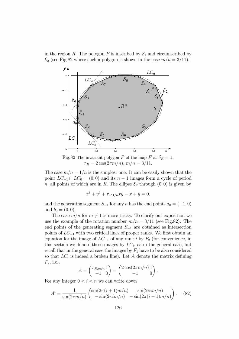
in the region R. The polygon P is inscribed by E1 and circumscribed byE2 (see Fig.82 where such a polygon is shown in the case m/n = 3/11).

Fig.82 The invariant polygon P of the map F at δR = 1,τR = 2 cos(2πm/n), m/n = 3/11.

The case m/n = 1/n is the simplest one: It can be easily shown that thepoint LC−1 ∩ LC0 = (0, 0) and its n − 1 images form a cycle of periodn, all points of which are in R. The ellipse E2 through (0, 0) is given by

x2 + y2 + τR,1/nxy − x+ y = 0,

and the generating segment S−1 for any n has the end points a0 = (−1, 0)and b0 = (0, 0).The case m/n for m 6= 1 is more tricky. To clarify our exposition we

use the example of the rotation number m/n = 3/11 (see Fig.82). Theend points of the generating segment S−1 are obtained as intersectionpoints of LC−1 with two critical lines of proper ranks. We first obtain anequation for the image of LC−1 of any rank i by F2 (for convenience, inthis section we denote these images by LCi, as in the general case, butrecall that in the general case the images by F1 have to be also consideredso that LCi is indeed a broken line). Let A denote the matrix definingF2, i.e.,

A =

µτR,m/n 1−1 0

¶=

µ2 cos(2πm/n) 1

−1 0

¶.

For any integer 0 < i < n we can write down

Ai =1

sin(2πm/n)

µsin(2π(i+ 1)m/n) sin(2πim/n)− sin(2πim/n) − sin(2π(i− 1)m/n)

¶. (82)

126

(Note that for i = n we get an identity matrix). Making a properchange of coordinates and using (82) we get the following equation forthe straight line LCi for 0 ≤ i < n :

LCi : y = − sin(2πim/n)

sin(2π(i+ 1)m/n)x+

tan(π(i+ 1)m/n)

2 tan(πm/n)− 12.

The point of intersection of LC−1 and LCi has the following coordinates:µ0,tan(π(i+ 1)m/n)

2 tan(πm/n)− 12

¶. (83)

Nowwe need to determine the proper rank k1 such that the side Sk1 ⊂LCk1 of the polygon P is an upper adjacent segment of the generatingsegment S−1. The number n which is the period of the m/n-cycle, canbe written as n = rm + l, where an integer r = bn/mc is the numberof periodic points visited for one turn around the fixed point, and aninteger l < m is the rest. For our example m/n = 3/11 we have r = 3and l = 2. Following some geometrical reasoning, which we omit here,one can get that if (m− 1)/l is an integer, then

k1 =(m− 1)r

l, (84)

so that the coordinates of the point b0 are determined through m and nby substituting i = k1 into (83). It can be easily shown that the coor-dinates of the other end point a0 of S−1 are determined by substitutingi = k2 into (83), where

k2 = n− 2− k1. (85)

For the example shown in Fig.82 we have k1 = 3 and k2 = 6, so that theend points of S−1 are a0 = LC−1 ∩ LC6 and b0 = LC−1 ∩ LC3, whosecoordinates are obtained by substituting m/n = 3/11 and, respectively,i = 6 and i = 3 into (83).If (m− 1)/l is not an integer number, then we use a numerical algo-

rithm to determine k1 as the rank of the critical line whose intersectionwith LC−1 is m/n-periodic point; k2 is determined by (85) as before.Obviously, such a polygon P can be constructed for any rotation

number m/n. Summarizing we can state the following

Proposition. Let δR = 1, τR = τR,m/n given in (80). Then inthe phase space of the map F there exists an invariant polygon P with nedges whose boundary is made up by the generating segment S−1 ⊂ LC−1and its n− 1 images Si = F2(Si−1) ⊂ LCi, i = 0, ..., n − 2. Any initialpoint (x0, y0) ∈ P is periodic with rotation number m/n.

127

Up to now we have not discussed the behavior of a trajectory withan initial point (x0, y0) not belonging to the invariant region (either Por Q), which obviously depends on the parameters δL, τL of the map F1.Such a behavior can be quite rich, even in the case we are restricted to,that is for (δL, τL) ∈ SL in which the fixed point L

∗of F1 is attracting

being virtual for F . Without going into a detailed description we givehere different examples: A trajectory initiated outside P or Q can be

- attracted to a periodic or quasiperiodic trajectory belonging tothe boundary of the invariant region (as, for example, for δL = 0.3,τL = −0.4, when F is invertible, L

∗is a focus);

- mapped inside the invariant region (it is possible if F is (Z0 − Z2)- noninvertible, like, for example, for δL = −0.5, τL = 0.3; L∗ is a flipnode);- mapped to the boundary of the invariant region (it is possible for

(Z0−Z∞−Z1) - noninvertibility, for example, at δL = 0, τL = −0.3; L∗is a flip node);- attracted to some other attractor, regular, i.e., periodic or quasi-

periodic (e.g., to a periodic attractor for τR = 0.25, δL = 0.9, τL = −0.7)or chaotic (e.g., for τR = −1.5, δL = 0.1, τL = 0.63), coexisting with theinvariant region (for both examples L

∗is a focus);

- divergent (e.g., for τR = −1.5, δL = 0.9, τL = −0.7; L∗ is a focus).In the following we investigate the dynamics of the map F ‘after’

the center bifurcation, that is for δR > 1. Among all the infinitely manyinvariant curves filling the invariant region (P or Q) at δR = 1, onlythe boundary of it survives, being modified, after the bifurcation, thatis for δR = 1+ ε at some sufficiently small ε > 0. Roughly speaking, theboundary of the former invariant region is transformed into an attractingclosed invariant curve C on which the map F is reduced to a rotation.Similar to the NS bifurcation occurring for smooth maps, we can usethe notion of rotation numbers: In case of a rational rotation numberm/n two cycles of period n with rotation number m/n are born at thecenter bifurcation, one attracting and one saddle, and the closure of theunstable set of the saddle cycle approaching points of the attracting cycleforms the curve C. In the piecewise linear case such a curve is not smooth,but a piecewise linear set, which in general has infinitely many cornerpoints accumulating at the points of the attracting cycle. Differentlyfrom the smooth case such a curve is born not in a neighborhood ofthe fixed point: Obviously, its position is defined by the distance of thefixed point from the critical line LC. Description of such a curve, borndue to the center bifurcation for some piecewise linear maps, as wellas proof of its existence in particular cases, can be found in [37], [112],[119], [108], [109]. Our main interest here is related to the bifurcation

128

structure of the (δR, τR)-parameter plane, namely, to the periodicityregions corresponding to the attracting cycles born due to the centerbifurcation.

8.3.2 Bifurcation Diagrams in the (δR, τR)-parameter plane

Before entering into some general considerations we present examples ofthe 2D bifurcation diagram in the (δR, τR)-parameter plane for differentvalues of δL and τL giving some comments on the bifurcation structureof the parameter plane. Note that each of these examples deserves moredetailed investigation being quite rich in a sense of possible bifurcationscenarios. Some properties of similar bifurcation diagrams for piecewiselinear and piecewise smooth dynamical systems were described, e. g., in[54], [112], [118], [108]. Referring to these papers, we recall here a fewproperties using our examples.

Fig.83 Two-dimensional bifurcation diargams of the map F in the(δR, τR)-parameter plane. In (a) δL = 0.25, τL = 0.5. F is invertible andL∗is an attracting focus. In (b) δL = −0.5, τL = 0.3. F is noninvertible, of

(Z0 − Z2)-type, and L∗is an attracting flip node.

In the bifurcation diagrams presented in Fig.83a,b the parameter re-gions corresponding to attracting cycles of different periods n, n ≤ 32,are shown in different colors (note that the periodicity regions relatedto attracting cycles with the same period n, but different rotation num-bers, say m1/n and m2/n, are shown by the same color). If one takesthe (δR, τR)-parameter point belonging to some m/n-periodicity region,denoted by Pm/n, then the corresponding map F has an attracting cycleof period n, which in general may be not the unique attractor. Some pe-riodicity regions are marked also by the corresponding rotation numbers.White region on these figures is related either to higher periodicities, orto chaotic trajectories. Gray color corresponds to divergent trajectories.Fig.83a presents the 2D bifurcation diagram for δL = 0.25, τL =

129

0.5. In such a case the map F is invertible (given that we considerδR > 1, see Property 1); L

∗is an attracting focus. Fig.83b presents

the bifurcation diagram at δL = −0.5, τL = 0.3 : For such parametervalues F is noninvertible, of (Z0 − Z2)-type; L

∗is an attracting flip

node (i.e. one negative eigenvalue exists). Recall that such bifurcationdiagrams representing qualitatively different dynamic regimes, reflectalso possible results of the border-collision bifurcation of the attractingfixed point of the map F occurring when µ changes from a negative toa positive value. For example, if we fix δL = 0.25, τL = 0.5, δR = 4,τL = 0.5 (the parameter point is inside the region P1/5 on Fig.83a),then for µ < 0 the map F has the attracting focus L∗ which at µ = 0undergoes the border-collision bifurcation resulting (for µ > 0) in theattracting and saddle cycles of period 5. First of all we recall that anissuing point for the periodicity region Pm/n is (δR, τR) = (1, τR,m/n),where τR,m/n is given in (80). In the vicinity of the bifurcation lineδR = 1 the periodicity regions are ordered in a way similar to thatof the Arnold tongues associated with the NS bifurcation occurring forsmooth maps. In short, the periodicity regions follow a summation rule,or Farey sequence rule, holding for the related rotation numbers (see,e.g., [87], [76]). In particular, according to this rule if, for example,r1 = m1/n1 and r2 = m2/n2 are two rotation numbers, associated atδR = 1 with τR = τR,r1 and τR = τR,r2, τR,r1 < τR,r2 , then there existsalso a value τR = τR,r3, τR,r1 < τR,r3 < τR,r2 , related to the rotationnumber r3 = (m1 + m2)/(n1 + n2), so that (δR, τR) = (1, τR,r3) is anemanating point for the region Pr3. To illustrate the summation rulesome periodicity regions are marked in Fig.83 by the rotation numbersof the related cycles.The kind of bifurcations associated with the boundaries of the peri-

odicity regions differs from the smooth case: It is known that the bound-aries of the Arnold tongues issuing from the Neimark-Sacker bifurcationcurve are related to saddle-node bifurcations, and the other boundariescorrespond to stability loss of the related cycle. While for piecewiselinear maps the boundaries of the periodicity regions issuing from thecenter bifurcation line correspond to so-called border-collision pair bi-furcations (a piecewise linear analogue of the saddle-node bifurcation),which we shall consider in detail in the next section.Note also that differently from the smooth case the periodicity re-

gions can have a ‘sausage’ structure (see Fig.83) with several subregions,first described in [54], which is typical for piecewise smooth and piece-wise linear systems (see also [118], [112]). In fact, different subregionsof the same periodicity region for the considered map F are related todifferent compositions of the maps F1 and F2 applied to get the corre-

130

sponding cycle (attracting or saddle). It can be shown that the first(leftmost) subregion of the m/n-periodicity region, denoted by P 1

m/n, isrelated to an attracting m/n-cycle with two periodic points located inL and n− 2 points in R, that is, the related composition can be writtenas F n = F 2

1 F n−22 for m = 1, and Fn = F1 F i

2 F1 F n−2−i2 , for m 6= 1,

where i > 1 depends on m and n. The corresponding saddle m/n-cyclefor any m for parameters from P 1

m/n has one periodic point in L andn− 1 points in R, that is, for such a cycle Fn = F1 Fn−1

2 .

Fig.84 Bifurcation diagram for δR ∈ [1.9, 2.05] , δL = 0.5, τL = 0.25,related to the parameter path shown in Fig.83a by the thick straight linewith an arrow. The points of the attracting and saddle cycles are shown in

red and blue, respectively.

The ‘waist’ points separating subregions are related to a particular border-collision bifurcation at which points of the attracting and saddle cyclesexchange their stability colliding with the border: Namely, after thecollision the former attracting cycle becomes a saddle one while thesaddle cycle becomes attracting (for details see [31], [112]). To illus-trate such a border-collision bifurcation we have chosen the waist point(δR, τR) ≈ (2,−0.6666) of the region P1/4 at δL = 0.5, τL = 0.25 (seeFig.83a). Fig.84 presents a bifurcation diagram for δR ∈ [1.9, 2.05] ,τR = −1.6665δR+2.66635, so that the parameter point moves from thefirst subregion P 1

1/4, to the second one, denoted P 21/4 (the related para-

meter path is shown by the thick straight line with an arrow in Fig.83a).On this diagram the points of the attracting and saddle cycles are shownin red and blue, respectively. Three (x, y)-planes shown in gray representa part of the phase portrait of the system: Before the bifurcation, i.e.,for (δR, τR) ∈ P 1

1/4; at the moment of the border-collision related to thewaist point (δR, τR) ≈ (2,−0.6666); and after the bifurcation, i.e., for(δR, τR) ∈ P 2

1/4. Comparing the phase portrait related to the subregion

131

P 21/4 with the one related to P11/4, one can see that the number of periodic

points in L is increased: Now three points of the attracting cycle are inL and one in R, and for the saddle cycle we have two points in L andtwo in R.Let us comment also the overlapping of periodicity regions, which

corresponds to multistability (as an example, see Fig.83a on which sev-eral multistability regions are dashed, related with the periodicity re-gions P1/3 and P1/4. Some other overlapping zones can be seen in thesame figure, as well as in Fig.83b). Recall that considering the initialproblem of the BCB of the fixed point of F , we have that in the caseof multistability, varying µ through 0, the fixed point bifurcates intoseveral attractors. As it was already mentioned, any invariant set of Fcontracts linearly with µ as µ tends to 0 collapsing to the origin at µ = 0.Among such invariant sets we have the basins of attraction of coexistingattractors which shrink to 0 as well. Thus, one cannot answer a priori towhich attractor the initial point will be attracted after the bifurcation.This gives a source of unpredictability of the results of the BCB. Thisproblem was posed first in [64], see also [34]. To give an example, we fixδL = 0.25, τL = 0.5, τR = −2 and will increase the value of δR start-ing from δR = 1.5, when the map F has attracting and saddle cyclesof period 3 (see the arrow in Fig.83a). At δR ≈ 1.64 a border-collisionpair bifurcation occurs giving birth to attracting and saddle cycles ofperiod 4, i.e., the parameter point enters the bistability region. Fig.85apresents a part of the phase portrait of the system at δR = 1.65 whenthere are coexisting attracting cycles of period 3 and 4 whose basins ofattraction, separated by the stable set of the period 4 saddle, are shownin yellow and green, respectively. The unstable set (shown in blue) ofthe saddle 3-cycle, approaching points of the attracting 3-cycle, forms asaddle-node connection which is wrinkled due to two negative eigenval-ues of the attracting 3 cycle. With further increasing δR the stable setof the period 3 saddle (shown in red) tends to get a tangency with itsunstable set. Indeed, at δR ≈ 1.68 a homoclinic bifurcation occurs af-ter which the saddle-node connection is destroyed. Another qualitativechange of the phase space occurs when the attracting 3-cycle undergoesa ‘flip’ bifurcation (an eigenvalue passing through −1) resulting in acyclic chaotic attractor of period 6. After pairwise merging of the piecesof the attractor it becomes a 3-piece cyclic chaotic attractor shown inFig.85b (for further details related to the ‘flip’ bifurcation in a piecewiselinear map see [78]). Note that the boundary separating the basins ofattraction is no longer regular as in Fig.85a but fractal. Such a basintransformation is a result of the homoclinic bifurcation of the saddle 4-cycle.

132

Fig.85 In (a) δL = 0.25, τL = 0.5, δR = 1.65, τR = −2. Attracting cyclesof periods 3 and 4 with their basins of attraction (shown in yellow and

green, respectively) separated by the stable set of the 4-saddle; The unstableset (in blue) of the 3-saddle forms a saddle-node connection which is near tobe destroyed by homoclinic tangency with the stable set (in red). In (b)δR = 2.2. Basins of attraction of the 3-piece cyclic chaotic attractor and

4-cycle are shown in yellow and green, respectively.

A contact with the fractal basin boundary leads to the disappearanceof the chaotic attractor at δR ≈ 2.25. Thus, in the considered sequenceof bifurcations, the attracting 4-cycle coexists first with the attracting3-cycle, then with the 6-piece chaotic attractor and finally with the 3-piece chaotic attractor. To illustrate the border-collision bifurcation ofthe fixed point of F in a case of multistability we present in Fig.86 abifurcation diagram for µ ∈ [−0.2 : 1], related to Fig.85b. The problemof multiple attractors and the role of homoclinic bifurcation is discussedin [119], [108].

Fig.86 Phase space (x, y) as µ changes in the interval µ ∈ [−0.2 : 1] atδL = 0.25, τL = 0.5, δR = 2.2, τR = −2. After the BCB at µ = 0 the

attractor in red is the attracting 4-cycle, while the attractor in black is the3-piece chaotic attractor.

133

8.3.3 1/n periodicity regions and their BCB boundaries

Let us consider now the first subregion, denoted by P 11/n, of the main

periodicity region P1/n. For such regions in the parameter space wecan get the analytic representations for their boundaries related to theBCB, that is, the two boundaries of the regions issuing from the centerbifurcation line, which we shall call BC boundaries for short. Note thatin general any periodicity region has two BC boundaries and may havealso other boundaries which are related to the stability loss of the cor-responding attracting cycle. Note that (similarly to the smooth case)inside a periodicity region it is not guaranteed the existence of a closedinvariant curve, which can be destroyed in several ways (for a list ofmechanisms of destruction of a closed invariant attracting curve in thepiecewise linear case see [108]).So let us consider a periodicity region P1/n and let (δR, τR) ∈ P 1

1/n.

Denote the related attracting and saddle cycles by p = p0, ..., pn−1 andp0 =

©p00, ..., p

0n−1ª, respectively. Let p0, pn−1 ∈ L and p1, ..., pn−2 ∈ R.

As for the saddle cycle, let p00 ∈ L and p01, ..., p0n−1 ∈ R.We shall see what

happens with these cycles if the (δR, τR)-parameter point crosses the twoBC boundaries of P 1

1/n. To illustrate our consideration we use an exampleshown in Fig.87a for δL = 0.25, τL = 0.5, i.e., (δR, τR) ∈ P 1

1/5 (seeFig.83a).We consider a fixed value δR = δ∗R inside the periodicity tongue,

such that the qualitative position of the periodic points in the (x, y)phase plane is presented in Fig.87a. Now let us increase the value of τR,then the point pn−1 of the cycle moves towards the critical line LC−1,so that at some τR = τ ∗R we have pn−1 ∈ LC−1 (and, as a consequence,p0 ∈ LC0) which indicates a BCB. It occurs not only for the attractingcycle: Indeed, also the saddle cycle undergoes the BCB, namely, atτR = τ ∗R we have p0n−1 ∈ LC−1, moreover, p0n−1 = pn−1, as well asall the other points of the cycles p and p0 are pairwise merging on thecritical lines of the proper ranks (see Fig.87c). In such a way the ‘saddle-node’ BCB occurs (not related to an eigenvalue equal to 1). The valueτR = τ ∗R corresponds to the (δR, τR)-parameter point crossing the upperboundary of P 11/n, which we denote by BC1/n(1). While if at the fixedδR = δ∗R the value τR is decreased, then p0 and p01 move towards thecritical line LC−1, so that at some τR = τ∗∗R we have p0 = p01 ∈ LC−1,thus one more ‘saddle-node’ BCB occurs (see Fig.87b), related to the(δR, τR)-parameter point crossing the lower boundary of P 1

1/n, denotedby BC1/n(2).

134

Fig.87 Examples of the ‘saddle-node’ BCB for (δR, τR)-parameter pointscrossing the boundaries of P 11/5 at δL = 0.25, τL = 0.5 : (a)

(δ∗R, τR) = (1.25, 0.65) ∈ P 11/5 ; (b) (δ

∗R, τ

∗∗R ) ∈ BC1/5(2) where

τ ∗∗R ≈ 0.575; (c) (δ∗R, τ ∗R) ∈ BC1/5(1) where τ ∗R ≈ 0.726.Independently on the way the parameters τR and δR are varying, the twoconditions for the BCB of the cycle p (at this moment we say nothingabout its stability before the bifurcation), are p0 ∈ LC−1 and p0 ∈ LC0,or, more precisely,

BC1/n(1) (x0, 0)=Fn−12 F1(x0, 0), (86)

BC1/n(2) (0, y0)=F1 F n−12 (0, y0), (87)

where (x0, y0) are coordinates of the point p0.Let the matrix defining the map F2 be denoted by A, that is

A =

µτR 1−δR 0

¶.

It is not difficult to note that Ai, i > 1, can be written as follows:

Ai =

µai ai−1

−δRai−1−δRai−2¶, (88)

where ai is a solution of the second order difference equation

ai − τRai−1 + δRai−2 = 0 (89)

with the initial conditions

a0 = 1, a1 = τR. (90)

We know that the eigenvalues of the corresponding characteristic equa-tion of (89) are complex-conjugate: λ1,2(R) =

³τR ±

pτ 2R − 4δR

´/2,

135

where τ 2R < 4δR, so the general solution of (89) with the initial condi-tions (90) can be written as

ai =³p

δR´iÃ

cos(2πi/n) +τRp

4δR − τ 2Rsin(2πi/n)

!.

For example, a2 = τ 2R − δR, a3 = τ 3R − 2τRδR, and so on.Now, to get the condition in (86) in terms of the parameters of the

system, we first shift the coordinate system so that the origin becomesthe fixed point of F2, that is we make a change of variables: x0 = x−x∗,y0 = y−y∗. Note that y∗ = −δRx∗. Then, in the new variables the mapsF1 and F2, say eF1 and eF2, become

eF1 :µ x0

y0

¶7→µ

τL(x0 + x∗) + y0 + y∗ + 1− x∗

−δL(x0 + x∗)− y∗

¶, x0 ≤ −x∗;

eF2 :µ x0

y0

¶7→µ

τRx0 + y0

−δRx0¶, x0 ≥ −x∗.

The equality (86) in the new variables is

(x00 − x∗, δRx∗) = eF n−12 eF1(x00 − x∗, δRx∗). (91)

Note that eF i2 can be written as

eF i2 :

µx0

y0

¶7→ Ai

µx0

y0

¶,

where Ai is given in (88). So, substituting (88) with i = n− 1 into (91)and equating the two expressions for x00, we get the equality

δRan−1 − an + 1

δLan−2 − τLan−1 + 1=

δRan−2 − an−1 + 1δLan−3 − τLan−2

which can be also written as

BC1/n(1) :an−1 + an−2 + ...+ a1 + 1

δLan−2 − τLan−1 + 1=

an−2 + an−3 + ...+ a1 + 1

δLan−3 − τLan−2.

(92)Similarly, the equality in (87) in the new variables (x0, y0) is written as

(−x∗, y00 + δRx∗) = eF1 eFn−1

2 (−x∗, y00 + δRx∗),

from which we get the equality

BC1/n(2) :δL(an−1 − 1) + δR

δLan−2 + 1=

τL(an−1 − 1)− δRan−2 + τR − 1τLan−2 − δRan−3

.

(93)

136

Fig.88 The border-collision bifurcation curves BC1/n(1) and BC1/n(2),n = 3, ..., 9; δL = 0, τL = 0.5.

For fixed values of the parameters δL and τL, the equalities (92) and(93) represent, in an implicit form, two curves in the (δR, τR)-parameterplane. As an example, in Fig.88 the curves BC1/n(1) and BC1/n(2) areplotted for n = 3, ..., 9, where δL = 0, τL = 0.5. Obviously, only partic-ular arcs of the curves given in (92) and (93) are related to the BCB ofthe attracting cycle. The end points of such arcs are the waist pointsissuing from the NS curve, being two intersection points of (92) and (93),and one of them belongs, obviously, to the center bifurcation line, i.e.,δR = 1, τR = τR,1/n = 2 cos(2π/n) (see (80)).For example, let us consider in more details the region P 1

1/4 at δL = 0,τL = 0.5 (see Fig.88). The BC boundaries of P 1

1/4 are given by

BC1/4(1) : τR−δR−τLδR+τLτRδR+τ 2R+τLτ2R+τLδ

2R+1 = 0, (94)

BC1/4(2) : −τLτR− τL+ δR− 1− τLτ2R+ τLδR+ δRτR = 0. (95)

For τL = 0.5 we can easily obtain the waist points, which are (δR, τR) =(1, 0) and (δR, τR) = (3,−1). We can also check that for the curveBC1/4(1) the derivative of τR with respect to δR, evaluated at (δR, τR) =(1, 0) is

τ 0R|(1)(δR,τR)=(1,0) =1− τL1 + τL

,

137

while for the curve BC1/4(2) we have

τ 0R|(2)(δR,τR)=(1,0) =τL + 1

τL − 1 =1

τ 0R|(1)(δR,τR)=(1,0)These two derivatives are not equal (in effect they are reciprocal), thusthe point (δR, τR) = (1, 0), which is an issuing point for the region P 1

1/4,is not a cusp point.

1/3 periodicity regionLet us consider in more details the region P1/3 in the (δR, τR)-parameterplane for (δL, τL) ∈ SL. Let p = p0, p1, p2 be a cycle of period 3 of themap F such that p0, p1 ∈ L and p2 ∈ R. Substituting n = 3 to (92) and(93) we get the equations for the BC boundaries of P1/3, which are thestraight lines in the (δR, τR)-parameter plane:

BC1/3(1) :

½τR = (δR − δRδL − 1− τL)/(δL + τL), for δL 6= −τL;δR = 1, for δL = −τL;

(96)

BC1/3(2) :

½τR = (−δRδL − δRτL + δL − 1)/(1 + τL), for τL 6= −1;δR = 1, for τL = −1.

(97)We can also obtain the equations defining the boundaries of the triangleof stability of the cycle p. Indeed, the map F 3 corresponding to theconsidered cycle is F 3 = F2 F 2

1 , for which the related eigenvalues η1,2are less then 1 in modulus for

½τR > (δR(τL − δ2L)− 1 + δLτL)/(τ

2L − δL),

τR > (δR(τL + δ2L) + 1 + δLτL)/(τ2L − δL),

for τ 2L > δL;½τR < (δR(τL − δ2L)− 1 + δLτL)/(τ

2L − δL),

τR < (δR(τL + δ2L) + 1 + δLτL)/(τ2L − δL),

for τ 2L < δL;

δR < 1δ2L,

(98)

so that the ‘flip’ bifurcation line denoted by Fl1/3 and related to η2 = −1,is given by

Fl1/3 :

½τR = (δR(τL − δ2L)− 1 + δLτL)/(τ

2L − δL), for τ 2L 6= δL;

δR = (δLτL − 1)/(δ2L − τL), for τ 2L = δL;(99)

the bifurcation line related to η1 = 1, denoted by T1/3 (a particular"transcritical" bifurcation in our examples, as we shall see), is given by

T1/3 :

½τR = (δR(τL + δ2L) + 1 + δLτL)/(τ

2L − δL), for τ 2L 6= δL;

δR = −(δLτL + 1)/(δ2L + τL), for τ 2L = δL;(100)

138

and by C1/3 we denote the center bifurcation line (related to¯η1,2¯= 1

for the complex-conjugate η1,2), which is given by

C1/3 : δR =1

δ2L, δL 6= 0. (101)

Thus, in the (δR, τR)-parameter plane we have 5 straight lines such thattwo of them, namely, BC1/3(1), BC1/3(2) are necessarily the boundariesof P1/3, while three others depend on δL and τL : All the three linesmay be involved as boundaries of P1/3, or only two of them, or only one.Note that it may also happen that P1/3 = ∅, as well as P1/3 may be anunbounded set (as, for example, in the case shown in Fig.88, in whichthe straight line BC1/3(1) is parallel to the straight line Fl1/3). All theabove cases can be classified depending on the values of δL and τL.Coming back to the initial problem of the BCB of the attracting fixed

point of F occurring for µ varying through 0 at some fixed values of theother parameters of the normal form (71), one can check analytically,using (96)-(101), whether an attracting cycle of period 3 is born due tothe bifurcation.

139

9 Appendix on the Myrber’s map.

In this Appendix we summarize some of the properties of the maps whichare topologically conjugated to the logistic map or Myrberg’s map T :x0 = x2 − b, say T : X → X, X = [q−11 , q1] where q1 is the fixed pointalways repelling for b ∈ [−1/4, 2]. The critical point is denoted as xc,and the absorbing interval is I = [T (xc), T 2(xc)].On the x-axis, the repelling cycles and their preimages and limit

points have a fractal organization when b ≥ b1s where b1s denotes theFeigenbaum point, i.e. the limit point of the first flip bifurcation se-quence of the 2−cycle of T . For each value of the parameter b, b ≥ b1s,the fractal structure of the map singularities is completely identified fromthe box-within-a-box bifurcation structure described in the years 1975 byMira (see [87] and references therein). Consider b (b ≥ b1s) such that themap has an attracting k−cycle C, then for the map T k this cycle gives kattracting fixed points Pi, i = 1, ..., k, each of them with an immediatebasin d0(Pi), and a total non connected basin d(Pi) = ∪n>0T−knd0(Pi).The total basins d(Pi) have a fractal structure, and a strange repeller Λi

belongs to the boundary of ∪kn=1d(Pi). For the map T this is reflectedin a cyclical property, so that the basin d(C) is the union of the k basinsand its fronties is a strange repeller Λ, i.e. an invariant set, T (Λ) = Λ,such that the restriction T : Λ→ Λ is chaotic (in the sense of Devaney,i.e. topological chaos with positive topological entropy). This frontier(on which the map is chaotic) if a set of zero measure in the interval X.For any value of b almost all the points x of the interval ]q−11 , q1[ (i.e.

apart from at most a set of points of zero Lebesgue measure) have thesame asymptotic behavior, which sometimes is called metric attractorAλ, due to this property, and independently on its nature. This metricattractor Aλ can only be one of the following three typologies ([24],[104]):(1) a k−cycle (of any period k ≥ 1, either stable (|S| < 1), or neutral

(|S| = 1);(2) a critical attractor (Acr)with Cantor like structure, of zero Lebesgue

measure;(3) k−cyclic chaotic intervals, k ≥ 1.In the case (1) the generic omega limit set ω(x) is equal to the omega

limit set of the critical point xc, and the trajectory of xc tends to thek−cycle, stable or neutral Aλ, ω(xc) = Aλ. In the case in which |S| = 1the cycle belongs to the frontier of its basin (or better, stable set). Inthe case in which |S| < 1 the cycle is an attractor of T . For b > b1s thefrontier of the basin of attraction is a strange repeller Λ, i.e. an invariantset, T (Λ) = Λ such that the restriction T : Λ → Λ is chaotic (in thesense of Devaney). This frontier (on which the map is chaotic) if a set

140

of zero measure in the interval X, and it is a topological repellor, i.e. arepelling set in the definition given above.In the case (2) the generic omega limit set ω(x) is equal to ω(xc) =

Acr and xc ∈ Acr. In this case T : Acr → Acr is chaotic, however Acr

is not a topological attractor, that is, an "attractor of T" in the usualdefinition, but an "attractor in Milnor’ sense" and its stable set is thewhole interval, so that we can say that it is globally attracting in theinterval.We recall that an invariant set is an "attractor in Milnor’ sense" when

its stable set has positive Lebesgue measure in the space of the map.In the case (3) the critical point xc is either periodic or preperiodic,

merging into a repelling cycle (|S| > 1), which is called a critical periodicorbit, and at this parameter value a homoclinic bifurcation of this cycleoccurs. The critical periodic orbit belongs to the chaotic intervals Aλ. Inthis case T : Aλ → Aλ is chaotic, and Aλ may be a topological attractoror an "attractor in Milnor’ sense" depending on the parameter value(for example, at the closure of a box of second kind it is a topologicalattractor, while at the closure of a box of first kind it is an attractor inMilnor’s sense, globally attracting in the whole interval).In all the cases (1), (2) and (3), the chaotic set is the closure of all

the repelling points in I.Noticing that in (2) and (3) above the chaotic sets attracts all the

points of the interval, we may generically speak of "chaotic attractors",but the chaotic set is of full measure only in the case (3).Let us define as bp the set of parameter values in the interval [−1/4, 2]

at which the typology (1) occurs, bcr and bch respectively the set ofparameter values in the same interval [−1/4, 2] at which the typology (2)and (3) respectively occurs. Then it is important to notice that the set bpconsists of infinitely many nontrivial intervals having a fractal structurein the interval [−1/4, 2] and dense in it (i.e. bp =[−1/4, 2]). The set bcris a completely disconnected set of zero Lebesgue measure while the setbch is a completely disconnected set of positive Lebesgue measure (forthe proofs we refer to Thunberg [2001] and references therein).Thus the set of points in the parameter space [−1/4, 2] in which we

have chaotic attracting sets of full measure in X is a set of positiveLebesgue measure.When the parameter b varies in the interval −1/4 ≤ b ≤ 2 sequences

of "boxes" occur, with the related bifurcations. Each box of the firstkind is opened by a fold bifurcation giving rise to a pair of cycles, sucha box of first kind closes when the cycle with S > 1 becomes critical forthe first time (i.e. the first time that a critical point merges in it, atits first homoclinic bifurcation). Inside each box of first kind the cycle

141

with S < 1 starts an infinite sequence of flip bifurcations, each of whichopens a box of second class which closes when it becomes critical forthe first time (i.e. at its first homoclinic bifurcation). Such sequences ofboxes have a fractal structure due to the self similar property. All theboundaries of boxes of first or second class are bifurcation values. Atall the opening values the map is of typology (1), while all the closurevalues are global (homoclinic) bifurcations (belonging to the set bch),and the map is of typology (3). Inside each box of first kind there existsa limit value of boxes of second kind at which the the map is of typology(2) (the so called Feigenbaum point). Particular bifurcation values of bare those which are limit points of other bifurcation values (for exampleboundaries of boxes of first class), such bifurcation values belong to theset bch and the map is of typology (3). In particular, when the criticalpoint xc is periodic or preperiodic the map is of typology (3).

142

10 Bibliography.

References

[1] Abraham R., L. Gardini, C. Mira "Chaos in Discrete Dynami-cal Systems (A visual introduction in 2 dimensions)", TELOS,Springer-Verlag, N-Y 1997.

[2] A. Agliari, G.I. Bischi and L. Gardini, Somemethods for thr GlobalAnalysis of Dynamic Games represented by Noninvertible Maps,Chapter 3 in Oligopoly and Complex Dynamics: Tools & Models,T. Puu and I. Sushko (eds.), Springer Verlag (in press).

[3] A. Agliari, Gardini, Puu (2005), Some global bifurcations relatedto the appearance of closed invariant curves, Computers and Math-ematics in Simulation 68, pp.201-219

[4] A. Agliari, Gardini, Puu (2006),Global bifurcation in duopolywhen the fixed point is destabilized via a subcritical Neimark bi-furcation, International Game Theory Review 8, pp. 1-20

[5] Agliari A. (2006), Homoclinic connections and subcritical Neimarkbifurcations in a duopoly model with adaptively adjusted produc-tions, Chaos Solitons & Fractals 29, pp. 739-755

[6] A. Agliari, G. I. Bischi, R. Dieci, L. Gardini (2005) “Global bi-furcations of closed invariant curves in two-dimensional maps: Acomputer assisted study” International Journal of Bifurcations andChaos, vol. 15 (4), pp. 1285-1328

[7] A. Agliari, G.I. Bischi, R. Dieci, L. Gardini (2006) “Homoclinictangles associated with closed invariant curves in families of 2Dmaps” Grazer Math. Ber. N. 350, pp. 1-14

[8] Agliari, Dieci (2006), Coexistence of attractors and homoclinicloops in a Kaldor-like business cycle model, In: T. Puu andI Sushko (eds.): Business cycle dynamics: Models and tools.Springer-Verlag, pp.223-254.

[9] Agliari A. (2007), On the bifurcation mechanisms causing the ap-pearance of invariant closed curves, Grazer Math. Ber., N.351, pp.1-20

[10] Agliari, Dieci, Gardini (2007), Homoclinic tangle in Kaldor’s likebusiness cycle models, Journal of Economic Behavior and Organi-zation 62, pp. 324-347

[11] A. Agliari, C. Chiarella, L. Gardini (2006) “A Re-evaluation ofthe Adaptive Expectations in Light of Global Nonlinear DynamicAnalysis ” Journal of Economic Behavior and Organization, Vol60/4, pp 526-552.

[12] V. Avrutin, M. Schanz. On fully developed bandcount adding sce-

143

nario. Nonlinearity 21 (2008), 1077-1103.[13] Azariadis, C. and Guesnerie, R., 1986, "Sunspots and cycles". Re-

view of Economic Studies 53, 725-736.[14] Banerjee, S. and C. Grebogi [1999] "Border-collision bifurcations

in two-dimensional piecewise smooth maps", Physical Review E,59, No. 4, 4052-4061.

[15] S. Banerjee, M.S. Karthik, G. Yuan and J.A. Yorke, Bifurcationsin One-Dimensional Piecewise Smooth Maps - Theory and Appli-cations in Switching Circuits, IEEE Trans. Circuits Syst.-I: Fund.Theory Appl. 47 No. 3 (2000), 389-394.

[16] Banerjee, S., Ranjan, P., and Grebogi, C., Bifurcations in 2DPiecewise Smooth Maps - Theory and Applications in SwitchingCircuits, IEEE Trans. Circuits Syst.-I: Fund. Theory Appl. 47 No.5 (2000), 633-64.

[17] Barnsley M.F. and S. Demko (1985): Iterated function systemsand the global construction of fractals. The Proceedings of theRoyal Society of London A399, 243-275.

[18] Barnsley M.F. "Fractals everywhere", Academic Press, CA,(1988).

[19] Bignami F., Agliari A. (2008) “Synchronization and on-off in-termittency phenomena in a market model with complementarygoods and adaptive expectations”Working paper n.51 del Diparti-mento di Scienze Economiche e Sociali, Serie verde “Metodi quan-titativi ed informatica” Università Cattolica, sede di Piacenza.

[20] Bischi, G.I., Mammana, C., Gardini, L., Multistability and cyclicattractors in duopoly games, Chaos Solitons & Fractals 11 (2000),543-564.

[21] G.I. Bischi, L. Gardini and M. Kopel, Analysis of Global Bifurca-tions in a Market Share Attraction Model, Journal of EconomicDynamics and Control, 24, pp. 855-879, (2000).

[22] G.I. Bischi and M. Kopel, Equilibrium Selection in a NonlinearDuopoly Game with Adaptive Expectations, Journal of EconomicBehavior and Organization, vol. 46/1, pp. 73-100, (2001).

[23] Bischi, G.I., Dieci, R., Rodano, G., and Saltari, E., 2001, "Multipleattractors and global bifurcations in a Kaldor-type business cyclemodel", Journal of Evolutionary Economics 11, pp.527-554.

[24] Blockh A.M. & M. Yu. Lyubich [1991] "Measurable dynamics ofS-unimodal maps of the interval", Ann. Scuola Norm. Sup. PisaCl. Sci.4, 24, pp. 545-573.

[25] Cass, D. and Shell, C., 1983, " Do sunspots matter?" Journal ofPolitical Economy 91. 193-227.

[26] Cournot, A.,.Researches into the principles of the theory of wealth.

144

Engl. transl., Chapter VII, 1963, Irwin Paperback Classics in Eco-nomics, (1838).

[27] R. Day, Irregular growth cycles, The American Economic Review72(3) (1982), 406-414.

[28] R. Day, “Complex Economic Dynamics”, MIT Press, Cambridge,1994.

[29] W. De Melo and S. van Strien, “One-Dimensional Dynamics”,Springer, New York , 1993.

[30] Devaney R., An Introduction to Chaotic Dynamical Systems,The Benjamin/Cummings Publishing Co., Menlo Park, Califor-nia, 1986.

[31] M. Di Bernardo, M.I. Feigen, S.J. Hogan and M.E. Homer, Localanalysis of C-bifurcations in n-dimensional piecewise smooth dy-namical systems, Chaos, Solitons & Fractals 10(11) (1999), 1881-1908.

[32] M. di Bernardo C.J. Budd A.R. Champneys P. Kowalczyk,Piecewise-smooth Dynamical Systems Theory and Applications,Springer-Verlag London, 2008.

[33] Dohtani, A., Misawa, T., Inaba, T., Yokoo, M., and Owase, T.,1996, "Chaos, complex transients and noise: Illustration with aKaldor model", Chaos Solitons & Fractals 7, pp.2157-2174.

[34] Dutta, M., Nusse, H. E., Ott, E., Yorke, J. A., and Yuan, G. H.[1999] "Multiple attractor bifurcations: A source of unpredictabil-ity in piecewise smooth systems", Phys. Rev. Lett. 83, 4281—4284.

[35] Feely, O., D. Fournier-Prunaret, I. Taralova-Roux, and D. Fitzger-ald [2000], "Nonlinear dynamics of bandpass sigma-delta modula-tion. An investigation by means of the critical lines tool", Inter-national Journal of Bifurcation and Chaos, 10(2), 303-327.

[36] Foroni I., Agliari A. (2008), Complex price dynamics in a financialmarket with imitation, Computational Economics 32, pp. 21-36

[37] Gallegati, M., Gardini, L., Puu, T., and Sushko, I., 2003, "Hicks’strade cycle revisited: cycles and bifurcations", Mathematics andComputers in Simulations, 63:505-527

[38] Ganguli, A. and S. Banerjee [2005] "Dangerous bifurcation at bor-der collision: when does it occur? ", Phys. Rev.E 71 057202 (1-4)

[39] Laura Gardini, Iryna Sushko and Ahmad Naimzada. GrowingThrough Chaotic Intervals. Journal of Economic Theory 143(2008), 541-557.

[40] Gardini L., "Homoclinic bifurcations in n-dimensional endomor-phisms, due to expanding periodic points”, Nonlinear Analysis,Theory, Methods & Applications, 23(8), pp. 1039-1089. 1994.

[41] Gardini, L., Puu, T. and Sushko, I.[2006], "The Hicksian Model

145

with Investment Floor and Income Ceiling". In: Business Cy-cles Dynamics. Models and Tools (T. Puu and I. Sushko Ed.s),Springer.Verlag, N.Y.

[42] Gardini, L., Puu, T., Sushko, I. [2006] "A Goodwin-type Modelwith a Piecewise Linear Investment Function". In: Business CyclesDynamics. Models and Tools (T. Puu and I. Sushko Ed.s), SpringerVerlag, N.Y.

[43] Gardini L., Cars Hommes, Fabio Tramontana, Robin de Vilder,2008, “Forward and Backward Dnamics in implicitly defined Over-lapping Generations Models” Journal of Economic Behavior andOrganization (to appear).

[44] Gaunersdorfer A., Hommes C.H., Wagener F.O.O. (2008), Bifur-cation routes to volatility clustering under evolutionary learning,Journal of Economic Behavior & Organization 67, pp. 27-47 JEBOforthcoming

[45] Grandmont, J.M., 1985, "On endogenous competitive business cy-cles". Econometrica 53, 995-1045.

[46] Grandmont, J.M. and Laroque, G., 1986, Stability of cycles andexpectations. Journal of Economic Theory 40, 138-151.

[47] Grandmont, J.M., 1993, "Expectations driven nonlinear businesscycles". In: RheinischwestfÄalische akademie der wissenschaften,vortrÄage N 397. Westdeutcher Verlag.

[48] Grasman, J., and Wentzel, J.J., 1994, "Coexistence of a limit cy-cle and an equilibrium in a Kaldor’s business cycle model and itsconsequences", Journal of Economic Behavior and Organization24, pp.369-377.

[49] Guckenheimer, J., On the bifurcaiton of maps on the interval,Invent. Math., 39 (1977), 165-178.

[50] Guckenheimer, J., Holmes, P., Nonlinear Oscillations, DynamicalSystems, and Bifurcations of Vector Fields, Springer-Verlag New-York 1983.

[51] Gumowski I. & Mira C. 1980 Dynamique chaotique. Transforma-tions ponctuelles. Transition ordre désordre, Cépadues Editions,Toulouse.

[52] Gumowski I. and Mira C., 1980, "Recurrences and discrete dy-namic systems", Lecture notes in Mathematics, Springer.

[53] C. Halse, M. Homer and M. di Bernardo, C-bifurcations andperiod-adding in one-dimensional piecewise-smooth maps, Chaos,Solitons & Fractals 18 (2003), 953-976.

[54] B.L. Hao, “Elementary Symbolic Dynamics and Chaos in Dissipa-tive Systems”, World Scientific, Singapore, 1989.

[55] Hao, B.-L., Zheng, W.-M., 1998, Applied Symbolic Dynamics and

146

Chaos, World Scientific[56] Hassouned, M.A., E.H. Abed and H.E. Nusse [2004] "Robust

dangerous Border-Collision Bifurcations in piecewise smooth sys-tems", Phys. Rev. Letters, 92(7) 070201 (1-4).

[57] Herrmann, R., 1985, "Stability and chaos in a Kaldor-type model",DP22, Department of Economics, University of Gottingen.

[58] Hicks, J.R., 1950, A Contribution to the Theory of the Trade Cycle,Clarendon Press, Oxford

[59] C.H. Hommes, H. Nusse, Period three to period two bifurcationsfor piecewise linear models, Journal of Economics 54(2) (1991)157-169.

[60] Ingram, W.T. 2002, "Invariant sets and inverse limits", Topologyand its Applications 126, pp. 393-408.

[61] Ingram, W.T. and W.S. Mahavier, 2004, "Interesting dynamicsand inverse limits in a family of one dimensional maps", AmericanMathematical Monthly, 111(3), pp. 198-215.

[62] Iooss, G., 1979, Bifurcation of Maps and Applications, North-Holland Publishing Company, Amsterdam.

[63] Iooss, G., and Joseph, D.D., 1980, Elementary Stability and Bifur-cation Theory, Springer-Verlag (New York).

[64] Kapitaniak, T. and Maistrenko, Yu. L. [1998] "Multiple choicebifurcations as a source of unpredictability in dynamical systems”Phys. Rev. E 58(4), 5161—5163.

[65] Kennedy, J.,A., Stockman, D.R. and Yorke J.A. 2007. Inverse lim-its and an implicitly defined difference equation from economics.Topology and its Applications 154, pp. 2533-2552

[66] Kennedy, J.,A. and Stockman, D.R., 2008. "Chaotic equilibria inmodels with backward dynamics". Journal of Economic Dynamicsand Control 32, 939-955.

[67] Kind, C., 1999, "Remarks on the economic interpretation of Hopfbifurcations", Economic Letters 62, pp.147-154.

[68] Kocic, V. L., Ladas, G., Global Behavior of Nonlinear DifferenceEquations of Higher Order with Applications, Kluwer AcademicPublishers 1993

[69] Kopel, M., Simple and complex adjustment dynamics in CournotDuopoly Models, Chaos, Solitons, and Fractals, 7, 2031-2048,(1996).

[70] Kuznetsov, Y. A. Elements of applied bifurcation theory, Springer-Verlag New-York 1998.

[71] Li T. and Yorke J.A. "Period Three Implies Caos", AmericanMathematical Monthly, 82, 985-992, (1975).

[72] Lines M., Westerhoff F. (2006), Expectations and the Multiplier-

147

Accelerator Model, In: T. Puu and I Sushko (eds.): Business cycledynamics: Models and tools. Springer-Verlag, pp.255-276

[73] Lines M. (2005), Bifurcation scenarios in a heterogeneous agent,multiplier-accelerator model, PUMA 16, pp.429-442

[74] Lorenz, H.W., 1992, "Multiple attractors, Complex Basin Bound-aries, and Transient Motion in Deterministic Economic Systems",in Dynamic Economic Models and Optimal Control, G. Feichtinger(Ed.), North-Holland, Amsterdam, pp.411-430

[75] Yu.L. Maistrenko, V.L. Maistrenko and L.O. Chua, Cycles ofchaotic intervals in a time-delayed Chua’s circuit, InternationalJournal of Bifurcation and Chaos 3(6) (1993), 1557-1572.

[76] Maistrenko Y.L., V.L. Maistrenko, S.I. Vikul and L. Chua [1995]"Bifurcations of attracting cycles from time-delayed Chua’s cir-cuit", International Journal of Bifurcation and Chaos 5(3), 653-671.

[77] Y.L. Maistrenko, V.L. Maistrenko and S.I. Vikul, On period-adding sequences of attracting cycles in piecewise linear maps,Chaos, Solitons & Fractals 9(1) (1998) 67-75.

[78] Maistrenko, Y., Sushko, I., and Gardini, L. [1998] "About twomechanisms of reunion of chaotic attractors", Chaos, Solitons &Fractals, 9(8), 1373-1390.

[79] Marotto F. R. (1978): “Snap-Back Repellers Imply Chaos in Rn

” Journal of Mathematical Analysis and Applications, 63(1), 199-223.

[80] Marotto, F. R. (2005): “On Redefining a Snap-Back Repeller,”Chaos, Solitons & Fractals, 25, 25-28.

[81] K. Matsuyama, Growing through cycles, Econometrica 67(2)(1999), 335-347.

[82] R.M. May "Simple mathematical models with very complicateddynamics" Nature, vol. 261, June 10 1976.

[83] Medio, A. and Raines, B., 2007, "Backward dynamics in eco-nomics. The inverse limit approach", Journal of Economic Dy-namics and Control 31, 1633-1671.

[84] Michener, R. and Ravikumar, B., 1998. Chaotic dynamics ina cash-in-advance economy. Journal of Economic Dynamics andControl 22, 1117—1137.

[85] Mira C. [1975] ”Accumulations de bifurcations et structures boîtes-emboîtées dans les récurrences et transformations ponctuelles.”Proceedings of the 7th International Conference On Nonlinear Os-cillations. Berlin sept. 1975. Akademic Verlag, Berlin 1977, BandI 2, 81-93.

[86] Mira C. [1976] ”Sur la double interprétation , déterministe et sta-

148

tistique, de certaines bifurcations complexes”. Comptes RendusAcad. Sc. Paris,. Série A, 283, 911-914.

[87] C. Mira, “Chaotic Dynamics”, World Scientific, Singapore, 1987.[88] Mira, C., Fournier-Prunaret, D., Gardini, L., Kawakami, H. and

Cathala, J.C.,.Basin bifurcations of two-dimensional noninvertiblemaps: fractalization of basins, International Journal of Bifurca-tions and Chaos, 4, 343-381, (1994).

[89] Mira C., L. Gardini, A. Barugola, J.C. Cathala "Chaotic Dynamicsin Two-Dimensional NonivertibIe Maps", World-Scientific Publ.Co., "Nonlinear Sciences, Series A", Singapore 1996.

[90] T. Mitra, A sufficient condition for topological chaos with an ap-plication to a model of endogenous growth, J. of Economic Theory,96, (2001), 133-152.

[91] A. Mukherji, Robust cyclical growth, International J. of EconomicTheory, 1 (2005), 233-246.

[92] Myrberg P. J. (1963) "Iteration von Quadratwurzeloperationen.III". Ann. Acad. Sci.. Fenn., ser. A, 336, 1-10.

[93] A. Norin and T. Puu, Cournot duopoly when the competitors op-erate under capacity constraints, Chaos, Solitons and Fractals 18(2003) 577-592

[94] H.E. Nusse and J.A. Yorke, Border-collision bifurcations includingperiod two to period three for piecewise smooth systems, Physica D57 (1992), 39-57.

[95] H.E. Nusse and J.A. Yorke, Border-collision bifurcations for piece-wise smooth one-dimensional maps, International Journal of Bi-furcation and Chaos 5(1) (1995), 189-207.

[96] T. Puu and I. Sushko Ed.s, “Oligopoly and Complex Dynamics:Models and Tools”, Springer, New York, 2002.

[97] T. Puu and I. Sushko Ed.s, “Business Cycles Dynamics: Modelsand Tools”, Springer, New York, 2006.

[98] Puu, T., Gardini, L., Sushko, I., 2005. A Hicksian multiplier-accelerator model with floor determined by capital stock. Journalof Economic Behavior and Organization 56, 331-348.

[99] Puu, T., 2007. The Hicksian trade cycle with floor and ceiling de-pendent on capital stock, Journal of Economic Dynamics & Con-trol 31:575-592.

[100] Rau, N., 1974, Trade Cycle: Theory and Evidence, Macmillan,London

[101] Reichlin, P., 1986, "Equilibrium cycles in an overlapping genera-tions economy with production", Journal of Economic Theory 40,89-102.

[102] Samuelson, P.A., 1939, "Interactions between the multiplier analy-

149

sis and the principle of acceleration", Review of Economics andStatistics 21: 75-78

[103] A.N. Sharkovsky (1964) "Coexistence of cycles of a continuousmap of a line into itself" Ukr. Math. Z. 16, pp.61-71.

[104] A.N. Sharkovsky, S.F. Kolyada, A.G. Sivak and V.V. Fedorenko,“Dynamics of One-dimensional Maps”, Kluwer Academic Publ.,Boston, 1997.

[105] Simpson, D. J. W., and Meiss, J. D., Neimark—Sacker Bifurcationsin Planar, Piecewise-Smooth, Continuous Maps, SIAM J. AppliedDynamical Systems, Vol. 7 (2008), No. 3, 795—824.

[106] I. Sushko, A. Agliari and L. Gardini, Bistability and border-collision bifurcations for a family of unimodal piecewise smoothmaps, Discrete and Continuous Dynamical Systems, Serie B, 5(3)(2005), 881-897.

[107] I. Sushko, A. Agliari and L. Gardini, Bifurcation Structure of Pa-rameter Plane for a Family of Unimodal Piecewise Smooth Maps:Border-Collision Bifurcation Curves, Chaos, Solitons & Fractals,29(3), (2006), 756-770.

[108] Sushko, I., and Gardini, L. [2006] "Center Bifurcation for a 2DPiecewise Linear Map". In: Business Cycles Dynamics. Modelsand Tools (T. Puu and I. Sushko Ed.s), Springer Verlag, N.Y.

[109] Sushko, I., and Gardini, L. Center Bifurcation for Two-Dimensional Border-Collision Normal Form, Int. J. Bifurcationand Chaos, Vol. 18, Issue 4 (2008), 1029-1050.

[110] Sushko, I., Gardini, L., Center Bifurcation of a point on thePoincaré Equator, Submitted to Grazer Mathematische Berichte(2009).

[111] Sushko, I., Gardini, L., and Puu, T., Tongues of Periodicity in aFamily of Two-dimensional Discontinuous Maps of Real MöbiusType, Chaos, Solitons & Fractals 21 (2004), 403-412.

[112] I. Sushko, T. Puu and L. Gardini, The Hicksian floor-roof model fortwo regions linked by interregional trade, Chaos Solitons & Fractals18 (2003), 593-612.

[113] Iryna Sushko, Laura Gardini and Tönu Puu: "Regular and ChaoticGrouwth Cyckles in a Hicksian Floor/Roof Model ", Journal ofEconomic Behavior and Organization. 2009 (to appear).

[114] F. Tramontana, L. Gardini and T. Puu “Duopoly games with al-ternative technologies”, JEDC, 33, pp. 250-265, 2008.

[115] F. Tramontana, L. Gardini “Use of homoclinic orbits and IteratedFunction Systems in backward models.” Grazer MathematischeBerichte, 2009 (to appear).

[116] Wiggins, S., 1988,Global Bifurcations and Chaos, Analytical Meth-

150

ods, Springer Verlag, New York.[117] Woodford, M., 1986, "Stationary sunspot equilibria in a finance

constrained economy", Journal of Economic Theory 40, 128—137.[118] Z.T. Zhusubaliyev and E. Mosekilde, “Bifurcations and Chaos in

Piecewise - Smooth Dynamical Systems”, World Scientific, Singa-pore, 2003.

[119] Zhusubaliyev, Z. T., Mosekilde, E., Maity, S., Mohanan, S., andBanerjee, S., Border collision route to quasiperiodicity: Numeri-cal investigation and experimental confirmation, Chaos 16, 023122(2006), 1-11.

[120] Zhusubaliyev, Z.T., E. Soukhoterin and E. Mosekilde [2007] "Qua-siperiodicity and torus breakdown in a power electronic dc/dc con-verter" Mathematics and Computers in Simulation 73, 364-377.

151