The Theory of Coarse-Graining also known as Non ...
204
The Theory of Coarse-Graining also known as Non-Equilibrium Statistical Mechanics PepEspa˜nol IWNET July 2015
Transcript of The Theory of Coarse-Graining also known as Non ...

The Theory of Coarse-Grainingalso known as
Non-Equilibrium Statistical Mechanics
Pep Espanol
IWNETJuly 2015

Intro Microdynamics Macrodynamics Examples Conclusions
Coarse-Graining
The art of using fewer degrees of freedom to describe asystem, but still retaining realism
2 / 74
The Theory of Coarse-Graining, also known as , Non-Equilibrium Statistical Mechanics

Intro Microdynamics Macrodynamics Examples Conclusions
Coarse-Graining
The art of using fewer degrees of freedom to describe asystem, but still retaining realism
2 / 74
The Theory of Coarse-Graining, also known as , Non-Equilibrium Statistical Mechanics

Intro Microdynamics Macrodynamics Examples Conclusions
Coarse-Graining
The art of using fewer degrees of freedom to describe asystem, but still retaining realism
2 / 74
The Theory of Coarse-Graining, also known as , Non-Equilibrium Statistical Mechanics

Intro Microdynamics Macrodynamics Examples Conclusions
Coarse-Graining
The art of using fewer degrees of freedom to describe asystem, but still retaining realism
2 / 74
The Theory of Coarse-Graining, also known as , Non-Equilibrium Statistical Mechanics

Intro Microdynamics Macrodynamics Examples Conclusions
Coarse-Graining
The art of using fewer degrees of freedom to describe asystem, but still retaining realism
2 / 74
The Theory of Coarse-Graining, also known as , Non-Equilibrium Statistical Mechanics

Intro Microdynamics Macrodynamics Examples Conclusions
Coarse-Graining
The art of using fewer degrees of freedom to describe asystem, but still retaining realism
2 / 74
The Theory of Coarse-Graining, also known as , Non-Equilibrium Statistical Mechanics

Intro Microdynamics Macrodynamics Examples Conclusions
Coarse-Graining
The art of using fewer degrees of freedom to describe asystem, but still retaining realism
A. Einstein: “Everything should be made as simple as possible,but not simpler”
2 / 74
The Theory of Coarse-Graining, also known as , Non-Equilibrium Statistical Mechanics

Intro Microdynamics Macrodynamics Examples Conclusions
Levels of description
Thermodynamics
Classical Mechanics
Fick
Langevin Dynamics Brownian Dynamics
Fluct Hydrodynamics
Consider a colloidal suspension.Each level of description
3 / 74
The Theory of Coarse-Graining, also known as , Non-Equilibrium Statistical Mechanics

Intro Microdynamics Macrodynamics Examples Conclusions
Levels of description
Thermodynamics
Classical Mechanics
Fick
Langevin Dynamics Brownian Dynamics
Fluct Hydrodynamics
Consider a colloidal suspension.Each level of description
is defined by a set ofrelevant variables
with characteristic timescales
3 / 74
The Theory of Coarse-Graining, also known as , Non-Equilibrium Statistical Mechanics
Intro Microdynamics Macrodynamics Examples Conclusions
Levels of description
Thermodynamics
Classical Mechanics
Fick
Langevin Dynamics Brownian Dynamics
Fluct Hydrodynamics
Consider a colloidal suspension.Each level of description
is defined by a set ofrelevant variables
with characteristic timescales
...well separated
3 / 74
The Theory of Coarse-Graining, also known as , Non-Equilibrium Statistical Mechanics

Intro Microdynamics Macrodynamics Examples Conclusions
Levels of description
4 / 74
The Theory of Coarse-Graining, also known as , Non-Equilibrium Statistical Mechanics
Intro Microdynamics Macrodynamics Examples Conclusions
Levels of description
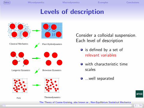
The challenge is toobtain the CGinteractions from the themicroscopic dynamic.
4 / 74
The Theory of Coarse-Graining, also known as , Non-Equilibrium Statistical Mechanics

Intro Microdynamics Macrodynamics Examples Conclusions
Levels of description
The challenge is toobtain the CGinteractions from the themicroscopic dynamic.
Run MD to find the CGinteractions
4 / 74
The Theory of Coarse-Graining, also known as , Non-Equilibrium Statistical Mechanics

Intro Microdynamics Macrodynamics Examples Conclusions
Non-Equilibrium Statistical Mechanics
Based on the concept of microstates and macrostates.
5 / 74
The Theory of Coarse-Graining, also known as , Non-Equilibrium Statistical Mechanics
Intro Microdynamics Macrodynamics Examples Conclusions
Non-Equilibrium Statistical Mechanics
Based on the concept of microstates and macrostates.
Objective: to obtain the dynamics of the macrostates from thedynamics of the microstates.
5 / 74
The Theory of Coarse-Graining, also known as , Non-Equilibrium Statistical Mechanics

Intro Microdynamics Macrodynamics Examples Conclusions
Outline
Microscopic dynamics
6 / 74
The Theory of Coarse-Graining, also known as , Non-Equilibrium Statistical Mechanics

Intro Microdynamics Macrodynamics Examples Conclusions
Outline
Microscopic dynamics
Macroscopic dynamics
6 / 74
The Theory of Coarse-Graining, also known as , Non-Equilibrium Statistical Mechanics
Intro Microdynamics Macrodynamics Examples Conclusions
Outline
Microscopic dynamics
Macroscopic dynamics
M. Green’s approach: the macro dynamics is a Markov process
6 / 74
The Theory of Coarse-Graining, also known as , Non-Equilibrium Statistical Mechanics
Intro Microdynamics Macrodynamics Examples Conclusions
Outline
Microscopic dynamics
Macroscopic dynamics
M. Green’s approach: the macro dynamics is a Markov processR. Zwanzig’s approach: exact macro dynamics from projectionoperators.
6 / 74
The Theory of Coarse-Graining, also known as , Non-Equilibrium Statistical Mechanics
Intro Microdynamics Macrodynamics Examples Conclusions
Outline
Microscopic dynamics
Macroscopic dynamics
M. Green’s approach: the macro dynamics is a Markov processR. Zwanzig’s approach: exact macro dynamics from projectionoperators.generic approach: when energy is a function of CG variables
6 / 74
The Theory of Coarse-Graining, also known as , Non-Equilibrium Statistical Mechanics

Intro Microdynamics Macrodynamics Examples Conclusions
Outline
Microscopic dynamics
Macroscopic dynamics
M. Green’s approach: the macro dynamics is a Markov processR. Zwanzig’s approach: exact macro dynamics from projectionoperators.generic approach: when energy is a function of CG variables
Examples:
6 / 74
The Theory of Coarse-Graining, also known as , Non-Equilibrium Statistical Mechanics
Intro Microdynamics Macrodynamics Examples Conclusions
Outline
Microscopic dynamics
Macroscopic dynamics
M. Green’s approach: the macro dynamics is a Markov processR. Zwanzig’s approach: exact macro dynamics from projectionoperators.generic approach: when energy is a function of CG variables
Examples:
Brownian motion
6 / 74
The Theory of Coarse-Graining, also known as , Non-Equilibrium Statistical Mechanics

Intro Microdynamics Macrodynamics Examples Conclusions
Outline
Microscopic dynamics
Macroscopic dynamics
M. Green’s approach: the macro dynamics is a Markov processR. Zwanzig’s approach: exact macro dynamics from projectionoperators.generic approach: when energy is a function of CG variables
Examples:
Brownian motionThermal blobs
6 / 74
The Theory of Coarse-Graining, also known as , Non-Equilibrium Statistical Mechanics

Microscopic dynamics

Intro Microdynamics Macrodynamics Examples Conclusions
Microscopic dynamicsFull atomistic description. The microstate of the system isz = qi , pi , i = 1, · · · ,N.
8 / 74
The Theory of Coarse-Graining, also known as , Non-Equilibrium Statistical Mechanics

Intro Microdynamics Macrodynamics Examples Conclusions
Microscopic dynamicsFull atomistic description. The microstate of the system isz = qi , pi , i = 1, · · · ,N.Hamilton’s equations
qi =∂H
∂pi
pi = −∂H
∂qi
The Hamiltonian
H(z) =
N∑
i
p2i
2mi
+ V (q1, · · · , qN)
r
V(r)
8 / 74
The Theory of Coarse-Graining, also known as , Non-Equilibrium Statistical Mechanics

Intro Microdynamics Macrodynamics Examples Conclusions
Microscopic dynamics
Hamilton’s equations can also be written as
qi
pi
=
0 1
−1 0
∂H∂qi
∂H∂pi
z = J∂H
∂z= −
∂H
∂zJ∂
∂zz = Lz
where L is the Liouville operator.The solution of Hamilton’s equation with initial condition z is
zt = expLtz = Ttz
9 / 74
The Theory of Coarse-Graining, also known as , Non-Equilibrium Statistical Mechanics

Intro Microdynamics Macrodynamics Examples Conclusions
Microscopic dynamics
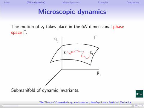
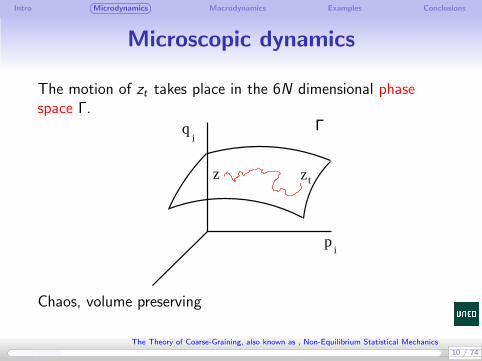
The motion of zt takes place in the 6N dimensional phasespace Γ.
10 / 74
The Theory of Coarse-Graining, also known as , Non-Equilibrium Statistical Mechanics

Intro Microdynamics Macrodynamics Examples Conclusions
Microscopic dynamics
The motion of zt takes place in the 6N dimensional phasespace Γ.
qi
pi
Γ
10 / 74
The Theory of Coarse-Graining, also known as , Non-Equilibrium Statistical Mechanics

Intro Microdynamics Macrodynamics Examples Conclusions
Microscopic dynamics
The motion of zt takes place in the 6N dimensional phasespace Γ.
qi
pi
Γ
z zt
10 / 74
The Theory of Coarse-Graining, also known as , Non-Equilibrium Statistical Mechanics

Intro Microdynamics Macrodynamics Examples Conclusions
Microscopic dynamics
The motion of zt takes place in the 6N dimensional phasespace Γ.
qi
pi
Γ
z zt
Noether theorem: symmetries in Hamiltonian lead toconserved quantities (energy, linear, angular momentum)
10 / 74
The Theory of Coarse-Graining, also known as , Non-Equilibrium Statistical Mechanics
Intro Microdynamics Macrodynamics Examples Conclusions
Microscopic dynamics
The motion of zt takes place in the 6N dimensional phasespace Γ.
qi
pi
Γ
z zt
Submanifold of dynamic invariants.
10 / 74
The Theory of Coarse-Graining, also known as , Non-Equilibrium Statistical Mechanics
Intro Microdynamics Macrodynamics Examples Conclusions
Microscopic dynamics
The motion of zt takes place in the 6N dimensional phasespace Γ.
qi
pi
Γ
z zt
Chaos, volume preserving
10 / 74
The Theory of Coarse-Graining, also known as , Non-Equilibrium Statistical Mechanics

Intro Microdynamics Macrodynamics Examples Conclusions
Statistical Mechanics
There is no way that we can specify the initial condition z ofa macroscopic sample of a system in an experiment.
11 / 74
The Theory of Coarse-Graining, also known as , Non-Equilibrium Statistical Mechanics

Intro Microdynamics Macrodynamics Examples Conclusions
Statistical Mechanics
There is no way that we can specify the initial condition z ofa macroscopic sample of a system in an experiment.
At most, we may specify the probability density of initialconditions ρ0(z) as a reflection of our ignorance.
ρ0(z)dz is the probability of finding the microstate in avolume dz around z .
The question is then: what is the probability density ρt(z) offinding the system at z at a later time?
Given by Liouville theorem
11 / 74
The Theory of Coarse-Graining, also known as , Non-Equilibrium Statistical Mechanics
Intro Microdynamics Macrodynamics Examples Conclusions
Statistical Mechanics
Liouville Theorem:
12 / 74
The Theory of Coarse-Graining, also known as , Non-Equilibrium Statistical Mechanics

Intro Microdynamics Macrodynamics Examples Conclusions
Statistical Mechanics
Liouville Theorem:
Tt MTtz
z
M
12 / 74
The Theory of Coarse-Graining, also known as , Non-Equilibrium Statistical Mechanics

Intro Microdynamics Macrodynamics Examples Conclusions
Statistical Mechanics
Liouville Theorem:
Tt MTtz
z
M
∫
M
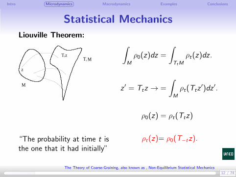
ρ0(z)dz =
∫
TtM
ρt(z)dz .
z ′ = Ttz → =
∫
M
ρt(Ttz′)dz ′.
ρ0(z) = ρt(Ttz)
ρt(z)= ρ0(T−tz).
12 / 74
The Theory of Coarse-Graining, also known as , Non-Equilibrium Statistical Mechanics
Intro Microdynamics Macrodynamics Examples Conclusions
Statistical Mechanics
Liouville Theorem:
Tt MTtz
z
M
“The probability at time t isthe one that it had initially”
∫
M
ρ0(z)dz =
∫
TtM
ρt(z)dz .
z ′ = Ttz → =
∫
M
ρt(Ttz′)dz ′.
ρ0(z) = ρt(Ttz)
ρt(z)= ρ0(T−tz).
12 / 74
The Theory of Coarse-Graining, also known as , Non-Equilibrium Statistical Mechanics

Intro Microdynamics Macrodynamics Examples Conclusions
Statistical Mechanics
Liouville Theorem:
Tt MTtz
z
M
Note that
ρt(z)= ρ0(T−tz)
implies
∂tρt(z) = Lρt(z)
Liouville equation
12 / 74
The Theory of Coarse-Graining, also known as , Non-Equilibrium Statistical Mechanics

Intro Microdynamics Macrodynamics Examples Conclusions
(Eq) Statistical Mechanics
“Experimental observation”: Many Hamiltonians are mixing
lımt→∞
ρt(z) = ρeq(z) = Φ(H(z))
for some Φ(E ), in weak sense.
13 / 74
The Theory of Coarse-Graining, also known as , Non-Equilibrium Statistical Mechanics

Intro Microdynamics Macrodynamics Examples Conclusions
(Eq) Statistical Mechanics
“Experimental observation”: Many Hamiltonians are mixing
lımt→∞
ρt(z) = ρeq(z) = Φ(H(z))
for some Φ(E ), in weak sense. Obviously, Lρeq = 0(stationarity)
“All microstates (with the same energy) are equiprobable(in the long run)”.
13 / 74
The Theory of Coarse-Graining, also known as , Non-Equilibrium Statistical Mechanics

Intro Microdynamics Macrodynamics Examples Conclusions
(Eq) Statistical Mechanics
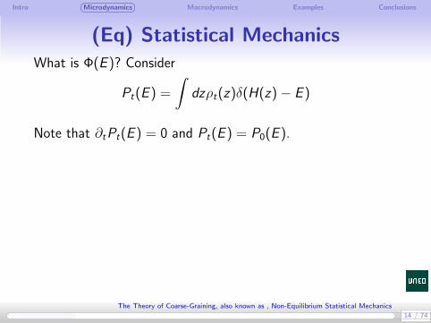
What is Φ(E )? Consider
Pt(E ) =
∫
dzρt(z)δ(H(z)− E )
14 / 74
The Theory of Coarse-Graining, also known as , Non-Equilibrium Statistical Mechanics
Intro Microdynamics Macrodynamics Examples Conclusions
(Eq) Statistical Mechanics
What is Φ(E )? Consider
Pt(E ) =
∫
dzρt(z)δ(H(z)− E )
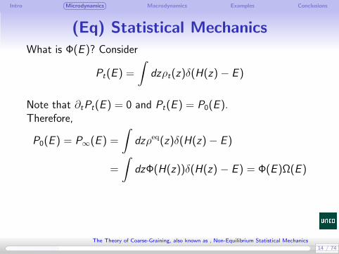
Note that ∂tPt(E ) = 0 and Pt(E ) = P0(E ).
14 / 74
The Theory of Coarse-Graining, also known as , Non-Equilibrium Statistical Mechanics
Intro Microdynamics Macrodynamics Examples Conclusions
(Eq) Statistical Mechanics
What is Φ(E )? Consider
Pt(E ) =
∫
dzρt(z)δ(H(z)− E )
Note that ∂tPt(E ) = 0 and Pt(E ) = P0(E ).Therefore,
P0(E ) = P∞(E ) =
∫
dzρeq(z)δ(H(z)− E )
=
∫
dzΦ(H(z))δ(H(z) − E ) = Φ(E )Ω(E )
14 / 74
The Theory of Coarse-Graining, also known as , Non-Equilibrium Statistical Mechanics

Intro Microdynamics Macrodynamics Examples Conclusions
(Eq) Statistical Mechanics
What is Φ(E )? Consider
Pt(E ) =
∫
dzρt(z)δ(H(z)− E )
Note that ∂tPt(E ) = 0 and Pt(E ) = P0(E ).Therefore,
P0(E ) = P∞(E ) =
∫
dzρeq(z)δ(H(z)− E )
=
∫
dzΦ(H(z))δ(H(z) − E ) = Φ(E )Ω(E )
where
Ω(E ) =
∫
dzδ(H(z)− E )
14 / 74
The Theory of Coarse-Graining, also known as , Non-Equilibrium Statistical Mechanics

Intro Microdynamics Macrodynamics Examples Conclusions
(Eq) Statistical Mechanics
The result is intuitive
ρeq(z) =P0(H(z))
Ω(H(z))
The probability of being at z is the probability that the systemhas the energy H(z) divided by the “number of microstates”compatible with that energy.
15 / 74
The Theory of Coarse-Graining, also known as , Non-Equilibrium Statistical Mechanics

Intro Microdynamics Macrodynamics Examples Conclusions
(Eq) Statistical Mechanics
The result is intuitive
ρeq(z) =P0(H(z))
Ω(H(z))
The probability of being at z is the probability that the systemhas the energy H(z) divided by the “number of microstates”compatible with that energy.If P0(E ) = δ(E − E0) we obtain the microcanonical ensemble
ρeq(z) =δ(H(z)− E0)
Ω(E0)
15 / 74
The Theory of Coarse-Graining, also known as , Non-Equilibrium Statistical Mechanics
Intro Microdynamics Macrodynamics Examples Conclusions
(Eq) Statistical Mechanics
Now a magical trick:The Principle of Maximum Entropy (PME)
16 / 74
The Theory of Coarse-Graining, also known as , Non-Equilibrium Statistical Mechanics

Intro Microdynamics Macrodynamics Examples Conclusions
(Eq) Statistical Mechanics
Now a magical trick:The Principle of Maximum Entropy (PME)Assume you know P(E ), but not ρ(z)
P(E ) =
∫
dzρ(z)δ(H(z) − E ) (1)
Many ρ(z) give the same P(E ). Which one is the “correct”one?
16 / 74
The Theory of Coarse-Graining, also known as , Non-Equilibrium Statistical Mechanics

Intro Microdynamics Macrodynamics Examples Conclusions
(Eq) Statistical Mechanics
Now a magical trick:The Principle of Maximum Entropy (PME)Assume you know P(E ), but not ρ(z)
P(E ) =
∫
dzρ(z)δ(H(z) − E ) (1)
Many ρ(z) give the same P(E ). Which one is the “correct”one?Consider the Gibbs-Jaynes entropy functional
S [ρ] = −kB
∫
dzρ(z) lnρ(z)
ρ0
PME: The least biased ρ(z) is the one that maximizes the GJentropy subject to (1).
16 / 74
The Theory of Coarse-Graining, also known as , Non-Equilibrium Statistical Mechanics

Intro Microdynamics Macrodynamics Examples Conclusions
(Eq) Statistical Mechanics
The solution is
ρ(z) =P(H(z))
Ω(H(z))
17 / 74
The Theory of Coarse-Graining, also known as , Non-Equilibrium Statistical Mechanics

Intro Microdynamics Macrodynamics Examples Conclusions
(Eq) Statistical Mechanics
The solution is
ρ(z) =P(H(z))
Ω(H(z))
identical to the “Experimental observation” !
17 / 74
The Theory of Coarse-Graining, also known as , Non-Equilibrium Statistical Mechanics

Intro Microdynamics Macrodynamics Examples Conclusions
(Eq) Statistical Mechanics
The solution is
ρ(z) =P(H(z))
Ω(H(z))
identical to the “Experimental observation” !
Therefore, the Principle of Maximum Entropy gives the samekind of “equiprobability” as mixing Hamiltonians.
17 / 74
The Theory of Coarse-Graining, also known as , Non-Equilibrium Statistical Mechanics

Intro Microdynamics Macrodynamics Examples Conclusions
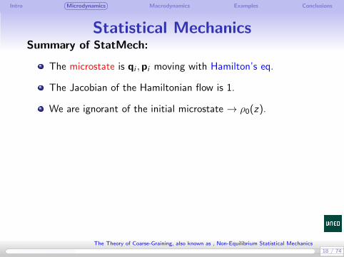
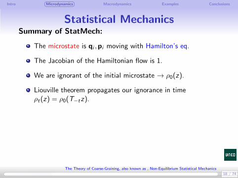
Statistical MechanicsSummary of StatMech:
The microstate is qi ,pi moving with Hamilton’s eq.
18 / 74
The Theory of Coarse-Graining, also known as , Non-Equilibrium Statistical Mechanics

Intro Microdynamics Macrodynamics Examples Conclusions
Statistical MechanicsSummary of StatMech:
The microstate is qi ,pi moving with Hamilton’s eq.
The Jacobian of the Hamiltonian flow is 1.
18 / 74
The Theory of Coarse-Graining, also known as , Non-Equilibrium Statistical Mechanics
Intro Microdynamics Macrodynamics Examples Conclusions
Statistical MechanicsSummary of StatMech:
The microstate is qi ,pi moving with Hamilton’s eq.
The Jacobian of the Hamiltonian flow is 1.
We are ignorant of the initial microstate → ρ0(z).
Liouville theorem propagates our ignorance in timeρt(z) = ρ0(T−tz).
18 / 74
The Theory of Coarse-Graining, also known as , Non-Equilibrium Statistical Mechanics

Intro Microdynamics Macrodynamics Examples Conclusions
Statistical MechanicsSummary of StatMech:
The microstate is qi ,pi moving with Hamilton’s eq.
The Jacobian of the Hamiltonian flow is 1.
We are ignorant of the initial microstate → ρ0(z).
Liouville theorem propagates our ignorance in timeρt(z) = ρ0(T−tz).
If mixing, at long times the system reaches an effectiveequilibrium ensemble in which all microstates areequiprobable.
This ensemble may also be obtained with the Principle ofMaximum Entropy.
18 / 74
The Theory of Coarse-Graining, also known as , Non-Equilibrium Statistical Mechanics

Macroscopic dynamics

Intro Microdynamics Macrodynamics Examples Conclusions
The dynamics of macrostates
Other names for macrostates:Macroscopic variables, slow variables, gross variables, collectivevariables, coarse-grained variables, reaction coordinates, orderparameters, internal variables, structural variables, etc.
20 / 74
The Theory of Coarse-Graining, also known as , Non-Equilibrium Statistical Mechanics

Intro Microdynamics Macrodynamics Examples Conclusions
The dynamics of macrostates
Other names for macrostates:Macroscopic variables, slow variables, gross variables, collectivevariables, coarse-grained variables, reaction coordinates, orderparameters, internal variables, structural variables, etc.The macrostates are phase functions A(z). There is a mapping
R6N → R
M
z → a = A(z)
20 / 74
The Theory of Coarse-Graining, also known as , Non-Equilibrium Statistical Mechanics

Intro Microdynamics Macrodynamics Examples Conclusions
The dynamics of macrostates
qi
pi
Γa aa0 1 2
21 / 74
The Theory of Coarse-Graining, also known as , Non-Equilibrium Statistical Mechanics

Intro Microdynamics Macrodynamics Examples Conclusions
The dynamics of macrostates
qi
pi
Γa aa0 1 2
21 / 74
The Theory of Coarse-Graining, also known as , Non-Equilibrium Statistical Mechanics

Intro Microdynamics Macrodynamics Examples Conclusions
The dynamics of macrostates
qi
pi
Γa aa0 1 2
Knowing a0 does notallow to predict the ma-crostate later!
21 / 74
The Theory of Coarse-Graining, also known as , Non-Equilibrium Statistical Mechanics

Intro Microdynamics Macrodynamics Examples Conclusions
The dynamics of macrostates
qi
pi
Γa aa0 1 2
Knowing a0 does notallow to predict the ma-crostate later!This implies a stochasticdescription and we needP(a, t)
21 / 74
The Theory of Coarse-Graining, also known as , Non-Equilibrium Statistical Mechanics

Intro Microdynamics Macrodynamics Examples Conclusions
The dynamics of macrostates
The relation between micro and macro probabilities
P(a, t) =
∫
dzρt(z)δ(A(z)− a)

Intro Microdynamics Macrodynamics Examples Conclusions
The dynamics of macrostates
The relation between micro and macro probabilities
P(a, t) =
∫
dzρt(z)δ(A(z)− a)
P(a, t) =
∫
dzρ0(z)δ(A(Ttz)− a)
22 / 74
The Theory of Coarse-Graining, also known as , Non-Equilibrium Statistical Mechanics

Intro Microdynamics Macrodynamics Examples Conclusions
The dynamics of macrostates
The relation between micro and macro probabilities
P(a, t) =
∫
dzρt(z)δ(A(z)− a)
P(a, t) =
∫
dzρ0(z)δ(A(Ttz)− a)
How do we specify the initial ensemble ρ0(z)?
22 / 74
The Theory of Coarse-Graining, also known as , Non-Equilibrium Statistical Mechanics

Intro Microdynamics Macrodynamics Examples Conclusions
The dynamics of macrostates
The relation between micro and macro probabilities
P(a, t) =
∫
dzρt(z)δ(A(z)− a)
P(a, t) =
∫
dzρ0(z)δ(A(Ttz)− a)
How do we specify the initial ensemble ρ0(z)?Assume that the only knowledge we have is the macroscopicP(a, 0).
PME: → ρ0(z) =P(A(z), 0)
Ω(A(z))
22 / 74
The Theory of Coarse-Graining, also known as , Non-Equilibrium Statistical Mechanics
Intro Microdynamics Macrodynamics Examples Conclusions
The dynamics of macrostates
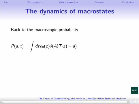
Back to the macroscopic probability
P(a, t) =
∫
dzρ0(z)δ(A(Ttz)− a)
23 / 74
The Theory of Coarse-Graining, also known as , Non-Equilibrium Statistical Mechanics

Intro Microdynamics Macrodynamics Examples Conclusions
The dynamics of macrostates
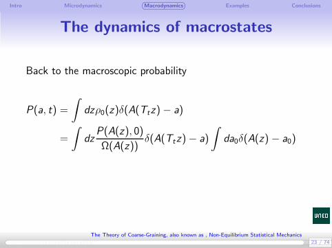
Back to the macroscopic probability
P(a, t) =
∫
dzρ0(z)δ(A(Ttz)− a)
=
∫
dzP(A(z), 0)
Ω(A(z))δ(A(Ttz)− a)
23 / 74
The Theory of Coarse-Graining, also known as , Non-Equilibrium Statistical Mechanics
Intro Microdynamics Macrodynamics Examples Conclusions
The dynamics of macrostates
Back to the macroscopic probability
P(a, t) =
∫
dzρ0(z)δ(A(Ttz)− a)
=
∫
dzP(A(z), 0)
Ω(A(z))δ(A(Ttz)− a)
∫
da0δ(A(z)− a0)
23 / 74
The Theory of Coarse-Graining, also known as , Non-Equilibrium Statistical Mechanics

Intro Microdynamics Macrodynamics Examples Conclusions
The dynamics of macrostates
Back to the macroscopic probability
P(a, t) =
∫
dzρ0(z)δ(A(Ttz)− a)
=
∫
dzP(A(z), 0)
Ω(A(z))δ(A(Ttz)− a)
∫
da0δ(A(z)− a0)
=
∫
da0P(a0, 0)1
Ω(a0)
∫
dzδ(A(z)− a0)δ(A(Ttz)− a)
=
∫
da0P(a0, 0)P(a0, 0|a, t)
This tells us how to evolve P(a, 0) → P(a, t).
23 / 74
The Theory of Coarse-Graining, also known as , Non-Equilibrium Statistical Mechanics
Intro Microdynamics Macrodynamics Examples Conclusions
The dynamics of macrostates
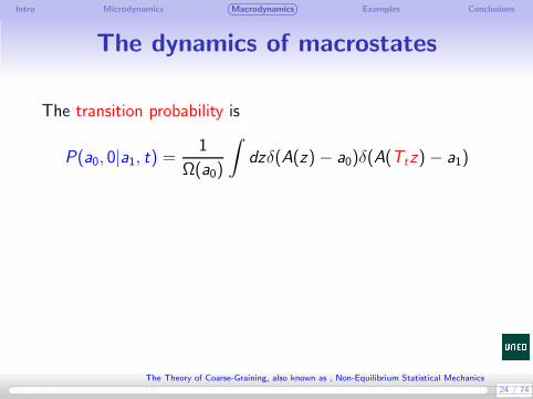
The transition probability is
P(a0, 0|a1, t) =1
Ω(a0)
∫
dzδ(A(z)− a0)δ(A(Ttz)− a1)
24 / 74
The Theory of Coarse-Graining, also known as , Non-Equilibrium Statistical Mechanics

Intro Microdynamics Macrodynamics Examples Conclusions
The dynamics of macrostates
The transition probability is
P(a0, 0|a1, t) =1
Ω(a0)
∫
dzδ(A(z)− a0)δ(A(Ttz)− a1)
This is the fundamental micro-macro link betweenmicroscopic and macroscopic dynamics.
(only assumption: initial microstates are equiprobable)
24 / 74
The Theory of Coarse-Graining, also known as , Non-Equilibrium Statistical Mechanics

Intro Microdynamics Macrodynamics Examples Conclusions
The dynamics of macrostates
The geometric interpretation is simple
P(a0, 0|a1, t) =
∫dzδ(A(z)− a0)δ(A(Ttz)− a1)
∫dzδ(A(z)− a0)
25 / 74
The Theory of Coarse-Graining, also known as , Non-Equilibrium Statistical Mechanics

Intro Microdynamics Macrodynamics Examples Conclusions
The dynamics of macrostates
The geometric interpretation is simple
P(a0, 0|a1, t) =
∫dzδ(A(z)− a0)δ(A(Ttz)− a1)
∫dzδ(A(z)− a0)
qi
pi
Γaa
10
25 / 74
The Theory of Coarse-Graining, also known as , Non-Equilibrium Statistical Mechanics

Intro Microdynamics Macrodynamics Examples Conclusions
The dynamics of macrostates
The geometric interpretation is simple
P(a0, 0|a1, t) =
∫dzδ(A(z)− a0)δ(A(Ttz)− a1)
∫dzδ(A(z)− a0)
qi
pi
Γaa
10
The transition probabi-lity is the fraction of mi-crostates of a0 that landon a1 after time t.
25 / 74
The Theory of Coarse-Graining, also known as , Non-Equilibrium Statistical Mechanics

Intro Microdynamics Macrodynamics Examples Conclusions
The dynamics of macrostates
Summary of Macrodynamics:
The dynamics of macrostates is necesarily stochastic P(a, t).
26 / 74
The Theory of Coarse-Graining, also known as , Non-Equilibrium Statistical Mechanics

Intro Microdynamics Macrodynamics Examples Conclusions
The dynamics of macrostates
Summary of Macrodynamics:
The dynamics of macrostates is necesarily stochastic P(a, t).
Macro probability P(a, t) =∫dzρ0(z)δ(A(Ttz)− a).
PME: Knowing P(a, 0) implies ρ0(z) =P(A(z),0)Ω(A(z)) .
The probability evolves P(a, t) =∫da0P(a, 0)P(a0, 0|a, t)
Micro-Macro dynamics link.
P(a0, 0|a, t) =1
Ω(a0)
∫
dzδ(A(z)− a0)δ(A(Ttz)− a)
26 / 74
The Theory of Coarse-Graining, also known as , Non-Equilibrium Statistical Mechanics

Intro Microdynamics Macrodynamics Examples Conclusions
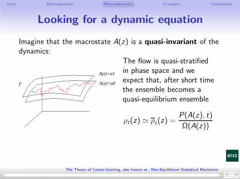
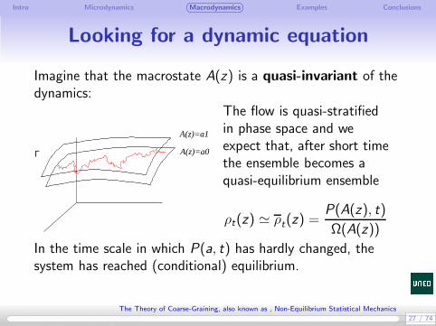
Looking for a dynamic equation
Imagine that the macrostate A(z) is a quasi-invariant of thedynamics:
27 / 74
The Theory of Coarse-Graining, also known as , Non-Equilibrium Statistical Mechanics

Intro Microdynamics Macrodynamics Examples Conclusions
Looking for a dynamic equation
Imagine that the macrostate A(z) is a quasi-invariant of thedynamics:
Γ
A(z)=a1
A(z)=a0
27 / 74
The Theory of Coarse-Graining, also known as , Non-Equilibrium Statistical Mechanics

Intro Microdynamics Macrodynamics Examples Conclusions
Looking for a dynamic equation
Imagine that the macrostate A(z) is a quasi-invariant of thedynamics:
Γ
A(z)=a1
A(z)=a0
27 / 74
The Theory of Coarse-Graining, also known as , Non-Equilibrium Statistical Mechanics
Intro Microdynamics Macrodynamics Examples Conclusions
Looking for a dynamic equation
Imagine that the macrostate A(z) is a quasi-invariant of thedynamics:
Γ
A(z)=a1
A(z)=a0
The flow is quasi-stratifiedin phase space and weexpect that, after short timethe ensemble becomes aquasi-equilibrium ensemble
ρt(z) ≃ ρt(z) =P(A(z), t)
Ω(A(z))
In the time scale in which P(a, t) has hardly changed, thesystem has reached (conditional) equilibrium.
27 / 74
The Theory of Coarse-Graining, also known as , Non-Equilibrium Statistical Mechanics

Intro Microdynamics Macrodynamics Examples Conclusions
Looking for a dynamic equation
The time derivative of the probability is
∂tP(a, t) =
∫
dz∂tρt(z)δ(A(z)− a)
28 / 74
The Theory of Coarse-Graining, also known as , Non-Equilibrium Statistical Mechanics

Intro Microdynamics Macrodynamics Examples Conclusions
Looking for a dynamic equation
The time derivative of the probability is
∂tP(a, t) =
∫
dz∂tρt(z)δ(A(z)− a)
=
∫
dzρt(z)Lδ(A(z)− a)
28 / 74
The Theory of Coarse-Graining, also known as , Non-Equilibrium Statistical Mechanics

Intro Microdynamics Macrodynamics Examples Conclusions
Looking for a dynamic equation
The time derivative of the probability is
∂tP(a, t) =
∫
dz∂tρt(z)δ(A(z)− a)
=
∫
dzρt(z)Lδ(A(z)− a)
= −∂
∂a
∫
dzρt(z)δ(A(z)− a)LA(z)
quasiequilibrium ≃ −∂
∂a
∫
dzP(A(z), t)
Ω(A(z))δ(A(z)− a)LA(z)
= −∂
∂av (a)P(a, t)
28 / 74
The Theory of Coarse-Graining, also known as , Non-Equilibrium Statistical Mechanics

Intro Microdynamics Macrodynamics Examples Conclusions
Looking for a dynamic equation
In the quasi-equilibrium approximation
∂tP(a, t) = −∂
∂av (a)P(a, t)
with the drift term is given by the microscopic expression
v (a) = 〈LA〉a =1
Ω(a)
∫
dzδ(A(z)− a)LA(z)
Wow! Closed equation for P(a, t) in microscopic terms!
29 / 74
The Theory of Coarse-Graining, also known as , Non-Equilibrium Statistical Mechanics

Intro Microdynamics Macrodynamics Examples Conclusions
Looking for a dynamic equation
Unfortunately, the quasi-equilibrium approximation is not verygood in general.
30 / 74
The Theory of Coarse-Graining, also known as , Non-Equilibrium Statistical Mechanics

Intro Microdynamics Macrodynamics Examples Conclusions
Looking for a dynamic equation
Unfortunately, the quasi-equilibrium approximation is not verygood in general.
It is a deterministic equation:
If P(a, 0) = δ(a − a0) then P(a, t) = δ(a − a(t))with a(t) = v (a(t)) and a(0) = a0 is the solution.
There is no widening of P(a, t)...
30 / 74
The Theory of Coarse-Graining, also known as , Non-Equilibrium Statistical Mechanics

Green’s approach to CG

Intro Microdynamics Macrodynamics Examples Conclusions
Green’s approachMelville Green 1952 proposed that the stochastic process ofmacrostates is a Markov process:
P(a1t1, a2, t2, . . . , antn) = P(a1, t1)P(a1, t1|a2, t2) · · ·P(an−1, tn−1|an, tn)
32 / 74
The Theory of Coarse-Graining, also known as , Non-Equilibrium Statistical Mechanics

Intro Microdynamics Macrodynamics Examples Conclusions
Green’s approachMelville Green 1952 proposed that the stochastic process ofmacrostates is a Markov process:
P(a1t1, a2, t2, . . . , antn) = P(a1, t1)P(a1, t1|a2, t2) · · ·P(an−1, tn−1|an, tn)
A mathematical result: for a continuum Markov process,the transition probability obeys the Fokker-Planck equation
∂
∂tP(a0t0|a, t) = −
∂
∂aD(1)(a)P(a0t0|a, t) +
1
2
∂2
∂a∂aD(2)(a)P(a0t0|a, t)
with initial condition
P(a0, t0|a, t0) = δ(a − a0)
32 / 74
The Theory of Coarse-Graining, also known as , Non-Equilibrium Statistical Mechanics
Intro Microdynamics Macrodynamics Examples Conclusions
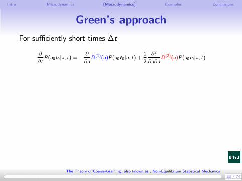
Green’s approach
For sufficiently short times ∆t
∂
∂tP(a0t0|a, t) = −
∂
∂aD(1)(a)P(a0t0|a, t) +
1
2
∂2
∂a∂aD(2)(a)P(a0t0|a, t)
33 / 74
The Theory of Coarse-Graining, also known as , Non-Equilibrium Statistical Mechanics

Intro Microdynamics Macrodynamics Examples Conclusions
Green’s approach
For sufficiently short times ∆t
∂
∂tP(a0t0|a, t) = −D(1)(a0)
∂
∂aP(a0t0|a, t) +D(2)(a0)
1
2
∂2
∂a∂aP(a0t0|a, t)
33 / 74
The Theory of Coarse-Graining, also known as , Non-Equilibrium Statistical Mechanics

Intro Microdynamics Macrodynamics Examples Conclusions
Green’s approach
For sufficiently short times ∆t
∂
∂tP(a0t0|a, t) = −D(1)(a0)
∂
∂aP(a0t0|a, t) +D(2)(a0)
1
2
∂2
∂a∂aP(a0t0|a, t)
Which is a diffusion equation with constant coefficients with aGaussian solution
P(a0, t0|a1, t0 +∆t)
= exp
−1
2∆t
(
a1 − a0 −∆tD(1)(a0))
D−1(2)
(a0)(
a1 − a0 −∆tD(1)(a0))
×1
(2π∆t)M/2 det(D(2)(a0))1/2
33 / 74
The Theory of Coarse-Graining, also known as , Non-Equilibrium Statistical Mechanics
Intro Microdynamics Macrodynamics Examples Conclusions
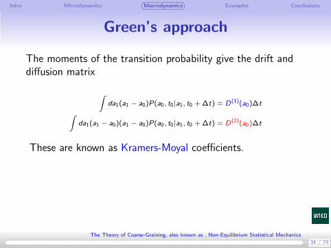
Green’s approach
The moments of the transition probability give the drift anddiffusion matrix
∫
da1(a1 − a0)P(a0, t0|a1, t0 +∆t) = D(1)(a0)∆t
∫
da1(a1 − a0)(a1 − a0)P(a0, t0|a1, t0 +∆t) = D(2)(a0)∆t
These are known as Kramers-Moyal coefficients.
34 / 74
The Theory of Coarse-Graining, also known as , Non-Equilibrium Statistical Mechanics

Intro Microdynamics Macrodynamics Examples Conclusions
Green’s approach
The moments of the transition probability give the drift anddiffusion matrix
∫
da1(a1 − a0)P(a0, t0|a1, t0 +∆t) = D(1)(a0)∆t
∫
da1(a1 − a0)(a1 − a0)P(a0, t0|a1, t0 +∆t) = D(2)(a0)∆t
These are known as Kramers-Moyal coefficients.Use the micro-macro link
P(a0, 0|a1, t) =1
Ω(a0)
∫
dzδ(A(z)− a0)δ(A(Ttz)− a1)
34 / 74
The Theory of Coarse-Graining, also known as , Non-Equilibrium Statistical Mechanics
Intro Microdynamics Macrodynamics Examples Conclusions
Green’s approach
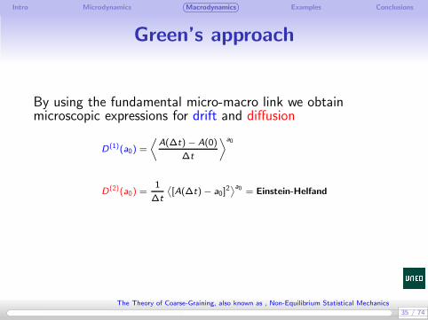
By using the fundamental micro-macro link we obtainmicroscopic expressions for drift and diffusion
D(1)(a0) =
⟨
A(∆t) − A(0)
∆t
⟩a0
D(2)(a0) =1
∆t
⟨
[A(∆t)− a0]2⟩a0 = Einstein-Helfand
35 / 74
The Theory of Coarse-Graining, also known as , Non-Equilibrium Statistical Mechanics
Intro Microdynamics Macrodynamics Examples Conclusions
Green’s approach
Summary of Green’s approach:
The dynamics of the macrostates is assumed to be describedby a Markov diffusion process.
36 / 74
The Theory of Coarse-Graining, also known as , Non-Equilibrium Statistical Mechanics

Intro Microdynamics Macrodynamics Examples Conclusions
Green’s approach
Summary of Green’s approach:
The dynamics of the macrostates is assumed to be describedby a Markov diffusion process.
The transition probability obeys the Fokker-Planck equation
The Fokker-Planck equation contains a drift and a diffusionterm
By using the fundamental micro-macro link the drift anddiffusion can be, in principle, computed from MD simulations.
36 / 74
The Theory of Coarse-Graining, also known as , Non-Equilibrium Statistical Mechanics

Zwanzig’s approach to CG
Intro Microdynamics Macrodynamics Examples Conclusions
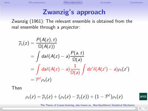
Zwanzig’s approachZwanzig (1961): The relevant ensemble is obtained from thereal ensemble through a projector :
ρt(z) =P(A(z), t)
Ω(A(z))
=
∫
daδ(A(z)− a)P(a, t)
Ω(a)
=
∫
daδ(A(z)− a)1
Ω(a)
∫
dz ′δ(A(z ′)− a)ρt(z′)
= P†ρt(z)
Then
ρt(z) = ρt(z) + (ρt(z)− ρt(z)) + (1− P†)ρt(z)
38 / 74
The Theory of Coarse-Graining, also known as , Non-Equilibrium Statistical Mechanics

Intro Microdynamics Macrodynamics Examples Conclusions
Zwanzig’s approachThe trick:
∂tρt(z) = ∂tP†ρt(z) = P†Lρt(z) + P†Lδρt(z)
∂tδρt(z) = Q†Lρt(z) = Q†Lρt(z) +Q†Lδρt(z)
The formal solution of the second Eq is
δρt(z) = expQ†Ltδρ0(z)︸ ︷︷ ︸
=0
+
∫ t
0
dt ′ expQ†L(t − t ′Q†Lρt′(z)
Inserting into the first equation leads to a closed equation forρt(z)
∂tρt(z) = P†Lρt(z) +
∫ t
0
dt ′P†L expQ†L(t − t ′Q†Lρt′(z)
39 / 74
The Theory of Coarse-Graining, also known as , Non-Equilibrium Statistical Mechanics

Intro Microdynamics Macrodynamics Examples Conclusions
Zwanzig’s approach
The final exact and closed equation for P(a, t) is
∂tP(a, t) = −∂
∂av(a)P(a, t)
+
∫ t
0dt′∫
da′Ω(a′)∂
∂aD(a, a′, t − t′)
∂
∂a′P(a′, t′)
Ω(a′)
40 / 74
The Theory of Coarse-Graining, also known as , Non-Equilibrium Statistical Mechanics

Intro Microdynamics Macrodynamics Examples Conclusions
Zwanzig’s approach
The final exact and closed equation for P(a, t) is
∂tP(a, t) = −∂
∂av(a)P(a, t)
+
∫ t
0dt′∫
da′Ω(a′)∂
∂aD(a, a′, t − t′)
∂
∂a′P(a′, t′)
Ω(a′)
Ω(a) =
∫
dzδ(A(z) − a)
v(a) = 〈LA〉a
D(a, a′, t) = 〈(LA − 〈LA〉a′
) expLQtδ(A − a)(LA− 〈LA〉a)〉a′
This is just a rewriting of Liouville’s theorem!!
40 / 74
The Theory of Coarse-Graining, also known as , Non-Equilibrium Statistical Mechanics

Intro Microdynamics Macrodynamics Examples Conclusions
Zwanzig’s approach
Markov approximation: The crucial approximation now isthe separation of time scales between A(z) and the memorykernel.
41 / 74
The Theory of Coarse-Graining, also known as , Non-Equilibrium Statistical Mechanics

Intro Microdynamics Macrodynamics Examples Conclusions
Zwanzig’s approach
Markov approximation: The crucial approximation now isthe separation of time scales between A(z) and the memorykernel.
t
D(t)
tt’=0
D(t-t’)
P(t)
t’
P(t’)
∫ t
0dt′D(t − t′)P(t′) ≈ P(t)
∫ ∞
0D(t′)dt′
D(t − t′) ≈ δ(t − t′)
∫ ∞
0D(t′′)dt′′
41 / 74
The Theory of Coarse-Graining, also known as , Non-Equilibrium Statistical Mechanics
Intro Microdynamics Macrodynamics Examples Conclusions
Zwanzig’s approach
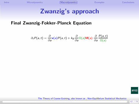
Final Zwanzig-Fokker-Planck Equation
∂tP(a, t) =∂
∂av(a)P(a, t) + kB
∂
∂aΩ(a)M(a)·
∂
∂a
P(a, t)
Ω(a)
42 / 74
The Theory of Coarse-Graining, also known as , Non-Equilibrium Statistical Mechanics

Intro Microdynamics Macrodynamics Examples Conclusions
Zwanzig’s approach
Final Zwanzig-Fokker-Planck Equation
∂tP(a, t) =∂
∂a
[
v(a) +M(a)·∂S
∂a(a)
]
P(a, t) + kB∂
∂aM(a)·
∂
∂aP(a, t)
42 / 74
The Theory of Coarse-Graining, also known as , Non-Equilibrium Statistical Mechanics

Intro Microdynamics Macrodynamics Examples Conclusions
Zwanzig’s approach
Final Zwanzig-Fokker-Planck Equation
∂tP(a, t) =∂
∂a
[
v(a) +M(a)·∂S
∂a(a)
]
P(a, t) + kB∂
∂aM(a)·
∂
∂aP(a, t)
Ω(a) =
∫
dzδ(A(z) − a) ∝ Peq(a) Equilibrium prob.
S(a)= kB lnΩ(a) Entropy
v(a) = 〈LA〉a Rev. Drift
M(a) =1
kB
∫ ∞
0dt′〈(LA − 〈LA〉a) expLt′(LA − 〈LA〉a)〉a Green-Kubo
This FPE is identical to the one obtained by Green. Inparticular Green-Kubo ⇔ Einstein-Helfand
42 / 74
The Theory of Coarse-Graining, also known as , Non-Equilibrium Statistical Mechanics

Intro Microdynamics Macrodynamics Examples Conclusions
Zwanzig’s approach
Summary of Zwanzig’s approach:
Exact equation obtained with a projection operator
43 / 74
The Theory of Coarse-Graining, also known as , Non-Equilibrium Statistical Mechanics

Intro Microdynamics Macrodynamics Examples Conclusions
Zwanzig’s approach
Summary of Zwanzig’s approach:
Exact equation obtained with a projection operator
The Markov property assumes a white noise model for theprojected current.
43 / 74
The Theory of Coarse-Graining, also known as , Non-Equilibrium Statistical Mechanics
Intro Microdynamics Macrodynamics Examples Conclusions
Zwanzig’s approach
Summary of Zwanzig’s approach:
Exact equation obtained with a projection operator
The Markov property assumes a white noise model for theprojected current.
The resulting equation is the FPE by Green
43 / 74
The Theory of Coarse-Graining, also known as , Non-Equilibrium Statistical Mechanics

generic

Intro Microdynamics Macrodynamics Examples Conclusions
The generic framework
When the Hamiltonian of the system is expressible in terms ofthe macrostates
H(z) = E (A(z))
then a powerful structure emerges.
45 / 74
The Theory of Coarse-Graining, also known as , Non-Equilibrium Statistical Mechanics

Intro Microdynamics Macrodynamics Examples Conclusions
The generic frameworkNote
LAµ(z) =∂Aµ
∂zJ0∂H
∂z=
∂Aµ
∂zJ0
∂E
∂aν(A(z))
∂Aν
∂z(z)
= Aµ,Aν∂E
∂aν(A(z))
46 / 74
The Theory of Coarse-Graining, also known as , Non-Equilibrium Statistical Mechanics

Intro Microdynamics Macrodynamics Examples Conclusions
The generic frameworkNote
LAµ(z) =∂Aµ
∂zJ0∂H
∂z=
∂Aµ
∂zJ0
∂E
∂aν(A(z))
∂Aν
∂z(z)
= Aµ,Aν∂E
∂aν(A(z))
then
vµ(a) = 〈LAµ〉a = Lµν(a)
∂E
∂aν(a)
where the reversible matrix is
Lµν(a) ≡
⟨∂Aµ
∂zJ0∂Aν
∂z
⟩a
= 〈Aµ,Aν〉a
46 / 74
The Theory of Coarse-Graining, also known as , Non-Equilibrium Statistical Mechanics

Intro Microdynamics Macrodynamics Examples Conclusions
The FPEThe Fokker-Planck Equation is
∂tP(a, t) =−∂
∂a
[[
L∂E
∂a+M
∂S
∂a
]
P(a, t)
]
+ kB∂
∂aM
∂
∂aP(a, t)
47 / 74
The Theory of Coarse-Graining, also known as , Non-Equilibrium Statistical Mechanics

Intro Microdynamics Macrodynamics Examples Conclusions
The FPEThe Fokker-Planck Equation is
∂tP(a, t) =−∂
∂a
[[
L∂E
∂a+M
∂S
∂a
]
P(a, t)
]
+ kB∂
∂aM
∂
∂aP(a, t)
Two theorems
M∂E
∂a= 0
∂E
∂aL∂S
∂a= kB
∂L
∂a
∂E
∂a
47 / 74
The Theory of Coarse-Graining, also known as , Non-Equilibrium Statistical Mechanics

Intro Microdynamics Macrodynamics Examples Conclusions
The FPEThe Fokker-Planck Equation is
∂tP(a, t) =−∂
∂a
[[
L∂E
∂a+M
∂S
∂a
]
P(a, t)
]
+ kB∂
∂aM
∂
∂aP(a, t)
Two theorems
M∂E
∂a= 0
L∂S
∂a= 0
47 / 74
The Theory of Coarse-Graining, also known as , Non-Equilibrium Statistical Mechanics
Intro Microdynamics Macrodynamics Examples Conclusions
The generic framework
Summary of the generic framework:
When the Hamiltonian may be expressed in terms of therelevant variables, generic emerges.
48 / 74
The Theory of Coarse-Graining, also known as , Non-Equilibrium Statistical Mechanics
Intro Microdynamics Macrodynamics Examples Conclusions
The generic framework
Summary of the generic framework:
When the Hamiltonian may be expressed in terms of therelevant variables, generic emerges.
There are a number of restrictions to be satisfied by anypossible model for the building blocks.
48 / 74
The Theory of Coarse-Graining, also known as , Non-Equilibrium Statistical Mechanics

Intro Microdynamics Macrodynamics Examples Conclusions
The generic framework
Summary of the generic framework:
When the Hamiltonian may be expressed in terms of therelevant variables, generic emerges.
There are a number of restrictions to be satisfied by anypossible model for the building blocks.
Typically, whenever you look for non-isothermal models, lookfor generic.
48 / 74
The Theory of Coarse-Graining, also known as , Non-Equilibrium Statistical Mechanics

Examples

Examples
Brownian Dynamics
Thermal Blobs
Examples
Brownian Dynamics
Thermal Blobs
Black box: “You give me the CG variables, I tell you how themove” (if...)
Intro Microdynamics Macrodynamics Examples Conclusions
Brownian Dynamics
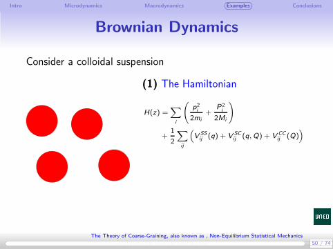
Consider a colloidal suspension
(1) The Hamiltonian
H(z) =∑
i
(
p2i
2mi
+P2i
2Mi
)
+1
2
∑
ij
(
V SSij (q) + V SC
ij (q,Q) + V CCij (Q)
)
50 / 74
The Theory of Coarse-Graining, also known as , Non-Equilibrium Statistical Mechanics

Intro Microdynamics Macrodynamics Examples Conclusions
Brownian Dynamics
Consider a colloidal suspension
(1) The Hamiltonian
H(z) =∑
i
(
p2i
2mi
+P2i
2Mi
)
+1
2
∑
ij
(
V SSij (q) + V SC
ij (q,Q) + V CCij (Q)
)
MD simulation unfeasible
(2) The relevant variables A(z) →H(z),Qi (Smoluchowski level)
50 / 74
The Theory of Coarse-Graining, also known as , Non-Equilibrium Statistical Mechanics
Intro Microdynamics Macrodynamics Examples Conclusions
Brownian Dynamics
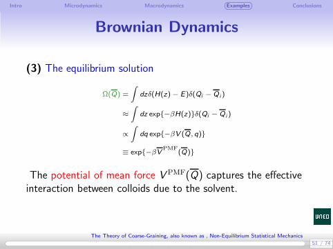
(3) The equilibrium solution
Ω(Q) =
∫
dzδ(H(z) − E)δ(Qi −Q i )
≈
∫
dz exp−βH(z)δ(Qi − Q i )
∝
∫
dq exp−βV (Q , q)
≡ exp−βVPMF
(Q)
The potential of mean force V PMF(Q) captures the effectiveinteraction between colloids due to the solvent.
51 / 74
The Theory of Coarse-Graining, also known as , Non-Equilibrium Statistical Mechanics

Intro Microdynamics Macrodynamics Examples Conclusions
Brownian Dynamics
The potential of mean force gives the mean force
FMFi (Q) = −
∂
∂Qi
VPMF
(Q)
= −∂
∂Qi
(
−kBT ln
∫
dq exp−βV (Q, q)
)
=
=
∫
dqexp−βV (Q, q)
∫dq exp−βV (Q, q)
[
−∂
∂Qi
V (Q, q)
]
= 〈Fi〉Q
52 / 74
The Theory of Coarse-Graining, also known as , Non-Equilibrium Statistical Mechanics

Intro Microdynamics Macrodynamics Examples Conclusions
Brownian Dynamics(4) The time derivative is LA → Vi
53 / 74
The Theory of Coarse-Graining, also known as , Non-Equilibrium Statistical Mechanics

Intro Microdynamics Macrodynamics Examples Conclusions
Brownian Dynamics(4) The time derivative is LA → Vi
(5) The drift term. The conditional expectation
〈. . .〉a =1
Ω(a)
∫
dzδ(A(z) − a) . . .
becomes
〈. . .〉Q =1
Ω(Q)
∫
dqdpdQdPδ(H(z) − E)δ(Q − Q) . . .
v(a) = 〈LA〉a is the conditional expectation of particle’smomentum. It vanishes by symmetry.
53 / 74
The Theory of Coarse-Graining, also known as , Non-Equilibrium Statistical Mechanics

Intro Microdynamics Macrodynamics Examples Conclusions
Brownian Dynamics(4) The time derivative is LA → Vi
(5) The drift term. The conditional expectation
〈. . .〉a =1
Ω(a)
∫
dzδ(A(z) − a) . . .
becomes
〈. . .〉Q =1
Ω(Q)
∫
dqdpdQdPδ(H(z) − E)δ(Q − Q) . . .
v(a) = 〈LA〉a is the conditional expectation of particle’smomentum. It vanishes by symmetry.(6) The friction matrix M(x) becomes the diffusion tensor.
Dij(Q) =1
kBT
∫ τ
0dt′〈ViVj(t
′)〉Q
53 / 74
The Theory of Coarse-Graining, also known as , Non-Equilibrium Statistical Mechanics

Intro Microdynamics Macrodynamics Examples Conclusions
Brownian Dynamics
(7) The dynamic equation is the Smoluchowski equation
∂tP(Q, t) =∂
∂Qi
[
Dij (Q)FMFj (Q)P(Q, t)
]
+ kBT∂
∂Qi
Dij(Q)·∂
∂Qj
P(Q, t)
equivalent to the SDE
dQi =∑
j
Dij(Q)FMFi (Q)dt + kBT
∑
j
∂Dij
∂Q j
(Q)dt + dQi
with the Fluctuation-Dissipation theorem
dQidQj = 2kBTDij (Q)dt
54 / 74
The Theory of Coarse-Graining, also known as , Non-Equilibrium Statistical Mechanics

Intro Microdynamics Macrodynamics Examples Conclusions
Brownian Dynamics
(8) Model, model, model:
Fi(Q) and Dij(Q) are many-body functions.
55 / 74
The Theory of Coarse-Graining, also known as , Non-Equilibrium Statistical Mechanics

Intro Microdynamics Macrodynamics Examples Conclusions
Brownian Dynamics
(8) Model, model, model:
Fi(Q) and Dij(Q) are many-body functions.
No way we can sample the 3M-dimensional space of Q’s
55 / 74
The Theory of Coarse-Graining, also known as , Non-Equilibrium Statistical Mechanics

Intro Microdynamics Macrodynamics Examples Conclusions
Brownian Dynamics
(8) Model, model, model:
Fi(Q) and Dij(Q) are many-body functions.
No way we can sample the 3M-dimensional space of Q’s
We will assume pair-wise forms.
55 / 74
The Theory of Coarse-Graining, also known as , Non-Equilibrium Statistical Mechanics

Intro Microdynamics Macrodynamics Examples Conclusions
Brownian Dynamics(8) Pair wise assumption
Fi (Q) =∑
j
〈Fij〉Q≈
∑
j
〈Fij〉Qij
Dij(Q)≈1
kBT
∫ τ
0dt′〈ViVj(t
′)〉Qij
56 / 74
The Theory of Coarse-Graining, also known as , Non-Equilibrium Statistical Mechanics

Intro Microdynamics Macrodynamics Examples Conclusions
Brownian Dynamics(8) Pair wise assumption
Fi (Q) =∑
j
〈Fij〉Q≈
∑
j
〈Fij〉Qij
Dij(Q)≈1
kBT
∫ τ
0dt′〈ViVj(t
′)〉Qij
For very dilute suspension, it is simple
Dij(Q) = δij1
kBT
∫ τ
0dt′〈ViVi (t
′)〉eq = δij1D0
For concentrated suspensions, the diffusion tensor describes allthe interactions mediated by the solvent.
56 / 74
The Theory of Coarse-Graining, also known as , Non-Equilibrium Statistical Mechanics

Intro Microdynamics Macrodynamics Examples Conclusions
Brownian Dynamics
(9) Micro→macro transfer of parameters.
Method 1: Run a short MD for two colloidal particles at agiven distance, compute average force and correlation of thefluctuations of the force. Repeat for other distances.
57 / 74
The Theory of Coarse-Graining, also known as , Non-Equilibrium Statistical Mechanics

Intro Microdynamics Macrodynamics Examples Conclusions
Brownian Dynamics
(9) Micro→macro transfer of parameters.
Method 1: Run a short MD for two colloidal particles at agiven distance, compute average force and correlation of thefluctuations of the force. Repeat for other distances.Method 2: Run a short MD for M fixed colloidal particles.Compute average force and correlation of the fluctuations ofthe force. Sort by distances.
The crucial point of the exercise is that we need to run shortsimulations to compute the mean force and diffusion tensor.
57 / 74
The Theory of Coarse-Graining, also known as , Non-Equilibrium Statistical Mechanics

Intro Microdynamics Macrodynamics Examples Conclusions
Thermal Blobs
58 / 74
The Theory of Coarse-Graining, also known as , Non-Equilibrium Statistical Mechanics
Intro Microdynamics Macrodynamics Examples Conclusions
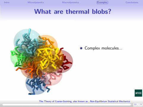
What are thermal blobs?
Complex molecules...
59 / 74
The Theory of Coarse-Graining, also known as , Non-Equilibrium Statistical Mechanics

Intro Microdynamics Macrodynamics Examples Conclusions
What are thermal blobs?
Complex molecules...
... described at a CG levelwith the CoM ...
59 / 74
The Theory of Coarse-Graining, also known as , Non-Equilibrium Statistical Mechanics

Intro Microdynamics Macrodynamics Examples Conclusions
What are thermal blobs?
Complex molecules...
... described at a CG levelwith the CoM ...
... and the internal energy
59 / 74
The Theory of Coarse-Graining, also known as , Non-Equilibrium Statistical Mechanics
Intro Microdynamics Macrodynamics Examples Conclusions
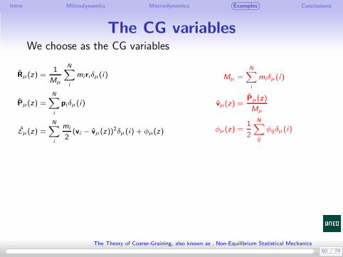
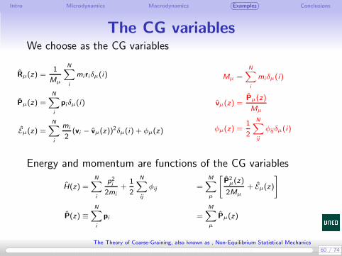
The CG variablesWe choose as the CG variables
Rµ(z) =1
Mµ
N∑
i
mi riδµ(i)
Pµ(z) =N∑
i
pi δµ(i)
Eµ(z) =N∑
i
mi
2(vi − vµ(z))
2δµ(i) + φµ(z)
Mµ =N∑
i
miδµ(i)
vµ(z) =Pµ(z)
Mµ
φµ(z) =1
2
N∑
ij
φijδµ(i)
60 / 74
The Theory of Coarse-Graining, also known as , Non-Equilibrium Statistical Mechanics
Intro Microdynamics Macrodynamics Examples Conclusions
The CG variablesWe choose as the CG variables
Rµ(z) =1
Mµ
N∑
i
mi riδµ(i)
Pµ(z) =N∑
i
pi δµ(i)
Eµ(z) =N∑
i
mi
2(vi − vµ(z))
2δµ(i) + φµ(z)
Mµ =N∑
i
miδµ(i)
vµ(z) =Pµ(z)
Mµ
φµ(z) =1
2
N∑
ij
φijδµ(i)
Energy and momentum are functions of the CG variables
H(z) =N∑
i
p2i
2mi
+1
2
N∑
ij
φij =M∑
µ
[
P2µ(z)
2Mµ+ Eµ(z)
]
P(z) ≡N∑
i
pi =M∑
µ
Pµ(z)
60 / 74
The Theory of Coarse-Graining, also known as , Non-Equilibrium Statistical Mechanics

Intro Microdynamics Macrodynamics Examples Conclusions
Time derivatives of CG variables
The time derivatives are
LRµ(z) = Vµ(z)
LPµ(z) =M∑
ν
Fµν(z)
LEµ(z) =M∑
ν
[
Qµν(z)−1
2Fµν(z)·Vµν(z)
]
Fµν(z) ≡N∑
ij
δµ(i)δν(j)Fij = −Fνµ(z)
Qµν(z) ≡N∑
ij
Fij
(
(vi − vµ) + (vj − vν)
2
)
δµ(i)δν(j) = −Qνµ(z)
61 / 74
The Theory of Coarse-Graining, also known as , Non-Equilibrium Statistical Mechanics

Intro Microdynamics Macrodynamics Examples Conclusions
The equilibrium probability
Peq(R,P, E) = Φ(E ,PT ) exp
1
kBS(R,P, E)
S(R, E) ≡ kB lnΩ(R, E)
Ω(R, E) =
∫
dz
M∏
µ
δ(Rµ − Rµ(z))δ(Pµ − Pµ(z))δ(Eµ − Eµ(z))
62 / 74
The Theory of Coarse-Graining, also known as , Non-Equilibrium Statistical Mechanics

Intro Microdynamics Macrodynamics Examples Conclusions
The conditional expectations
The conditional averages are of the form
〈· · · 〉RPE =1
Ω(α)
∫
dz
M∏
µ
δ(Rµ − Rµ(z))δ(Pµ − Pµ(z))δ(Eµ − Eµ(z)) · · ·
63 / 74
The Theory of Coarse-Graining, also known as , Non-Equilibrium Statistical Mechanics

Intro Microdynamics Macrodynamics Examples Conclusions
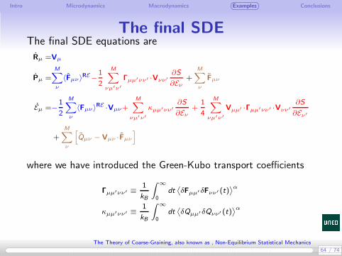
The final SDEThe final SDE equations are
Rµ =Vµ
Pµ =M∑
ν
〈Fµν〉RE−
1
2
M∑
νµ′ν′
Γµµ′νν′ ·Vνν′
∂S
∂Eν+
M∑
ν
Fµν
Eµ =−1
2
M∑
ν
〈Fµν〉RE ·Vµν+
M∑
νµ′ν′
κµµ′νν′
∂S
∂Eν+
1
4
M∑
νµ′ν′
Vµµ′ ·Γµµ′νν′ ·Vνν′
∂S
∂Eν′
+M∑
ν
[
Qµν − Vµν ·Fµν
]
64 / 74
The Theory of Coarse-Graining, also known as , Non-Equilibrium Statistical Mechanics
Intro Microdynamics Macrodynamics Examples Conclusions
The final SDEThe final SDE equations are
Rµ =Vµ
Pµ =M∑
ν
〈Fµν〉RE−
1
2
M∑
νµ′ν′
Γµµ′νν′ ·Vνν′
∂S
∂Eν+
M∑
ν
Fµν
Eµ =−1
2
M∑
ν
〈Fµν〉RE ·Vµν+
M∑
νµ′ν′
κµµ′νν′
∂S
∂Eν+
1
4
M∑
νµ′ν′
Vµµ′ ·Γµµ′νν′ ·Vνν′
∂S
∂Eν′
+M∑
ν
[
Qµν − Vµν ·Fµν
]
where we have introduced the Green-Kubo transport coefficients
Γµµ′νν′ ≡1
kB
∫ ∞
0dt⟨
δFµµ′ δFνν′ (t)⟩α
κµµ′νν′ ≡1
kB
∫ ∞
0dt⟨
δQµµ′ δQνν′ (t)⟩α
64 / 74
The Theory of Coarse-Graining, also known as , Non-Equilibrium Statistical Mechanics

Intro Microdynamics Macrodynamics Examples Conclusions
The final SDEThe final SDE equations are
Rµ =Vµ
Pµ =M∑
ν
〈Fµν〉RE−
1
2
M∑
νµ′ν′
Γµµ′νν′ ·Vνν′
∂S
∂Eν+
M∑
ν
Fµν
Eµ =−1
2
M∑
ν
〈Fµν〉RE ·Vµν+
M∑
νµ′ν′
κµµ′νν′
∂S
∂Eν+
1
4
M∑
νµ′ν′
Vµµ′ ·Γµµ′νν′ ·Vνν′
∂S
∂Eν′
+M∑
ν
[
Qµν − Vµν ·Fµν
]
Galilean invariant, conserve momentum and energy, randomterms satisfy Fluctuation-Dissipation
64 / 74
The Theory of Coarse-Graining, also known as , Non-Equilibrium Statistical Mechanics

Intro Microdynamics Macrodynamics Examples Conclusions
Model for the entropy
Whatever model for S(α) and 〈Fµν〉α should satisfy the
generic restriction
∂E
∂αL∂S
∂α= kB
∂L
∂α
∂E
∂α
which for the present CG description is
∂S
∂Rµ=
1
2
M∑
ν
Fµν
(
1
Tµ+
1
Tν
)
+ kB
M∑
ν
1
2
[
∂
∂Eµ+
∂
∂Eν
]
Fµν
This shows that the entropy plays now the role of a (minus)“potential of mean force”.
65 / 74
The Theory of Coarse-Graining, also known as , Non-Equilibrium Statistical Mechanics

Intro Microdynamics Macrodynamics Examples Conclusions
Model for the entropyRecall the definition of internal energy
Eµ(z) ≡N∑
i
mi
2(vi − vµ(z))
2δµ(i) +1
2
N∑
ij
φijδµ(i)
=N∑
i
mi
2(vi − vµ(z))
2δµ(i) +1
2
N∑
ij
φijδµ(j)δµ(i) +∑
ν 6=µ
1
2
N∑
ij
φijδν(j)δµ(i)
≈ E intµ (z) +
∑
ν 6=µ
Φµν(Rµν(z))
66 / 74
The Theory of Coarse-Graining, also known as , Non-Equilibrium Statistical Mechanics

Intro Microdynamics Macrodynamics Examples Conclusions
Model for the entropyRecall the definition of internal energy
Eµ(z) ≡N∑
i
mi
2(vi − vµ(z))
2δµ(i) +1
2
N∑
ij
φijδµ(i)
=N∑
i
mi
2(vi − vµ(z))
2δµ(i) +1
2
N∑
ij
φijδµ(j)δµ(i) +∑
ν 6=µ
1
2
N∑
ij
φijδν(j)δµ(i)
≈ E intµ (z) +
∑
ν 6=µ
Φµν(Rµν(z))
The entropy
S(R, E) ≡ kB ln
∫
dz
M∏
µ
δ(Rµ − Rµ(z))δ(Pµ − Pµ(z))δ(Eµ − Eµ(z))
= kB lnM∏
µ
∫
dzµδ(Rµ − Rµ(zµ))δ(Pµ − Pµ(z))δ(Eµ − Φµ − E intµ (z))
=∑
µ
Sµ(Eµ − Φµ(R))
66 / 74
The Theory of Coarse-Graining, also known as , Non-Equilibrium Statistical Mechanics

Intro Microdynamics Macrodynamics Examples Conclusions
Model for the entropyRecall the definition of internal energy
Eµ(z) ≡N∑
i
mi
2(vi − vµ(z))
2δµ(i) +1
2
N∑
ij
φijδµ(i)
=N∑
i
mi
2(vi − vµ(z))
2δµ(i) +1
2
N∑
ij
φijδµ(j)δµ(i) +∑
ν 6=µ
1
2
N∑
ij
φijδν(j)δµ(i)
≈ E intµ (z) +
∑
ν 6=µ
Φµν(Rµν(z))
The entropy is given by the sum of entropies of isolated blobs!
S(R, E) ≡ kB ln
∫
dz
M∏
µ
δ(Rµ − Rµ(z))δ(Pµ − Pµ(z))δ(Eµ − Eµ(z))
= kB lnM∏
µ
∫
dzµδ(Rµ − Rµ(zµ))δ(Pµ − Pµ(z))δ(Eµ − Φµ − E intµ (z))
=∑
µ
Sµ(Eµ − Φµ(R))
66 / 74
The Theory of Coarse-Graining, also known as , Non-Equilibrium Statistical Mechanics

Intro Microdynamics Macrodynamics Examples Conclusions
Model for the entropy
This model is OK, because it satisfies the generic restriction
∂S
∂Rµ=
1
2
M∑
ν
Fµν
(
1
Tµ+
1
Tν
)
+ kB
M∑
ν
1
2
[
∂
∂Eµ+
∂
∂Eν
]
Fµν
67 / 74
The Theory of Coarse-Graining, also known as , Non-Equilibrium Statistical Mechanics

Intro Microdynamics Macrodynamics Examples Conclusions
Model for the entropy
This model is OK, because it satisfies the generic restriction
∂S
∂Rµ=
1
2
M∑
ν
Fµν
(
1
Tµ+
1
Tν
)
+ kB
M∑
ν
1
2
[
∂
∂Eµ+
∂
∂Eν
]
Fµν
provided that the average force defined as
Fµν(R) = −∂Φµ
∂Rν
67 / 74
The Theory of Coarse-Graining, also known as , Non-Equilibrium Statistical Mechanics

Intro Microdynamics Macrodynamics Examples Conclusions
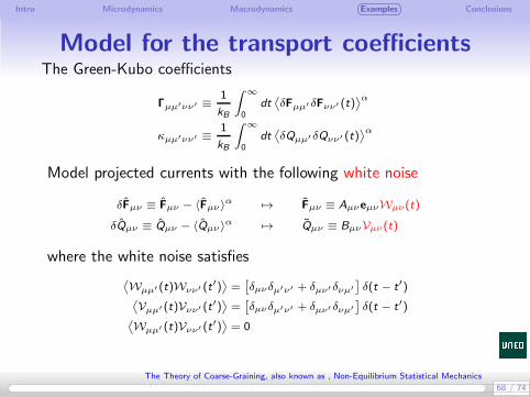
Model for the transport coefficientsThe Green-Kubo coefficients
Γµµ′νν′ ≡1
kB
∫ ∞
0dt⟨
δFµµ′ δFνν′ (t)⟩α
κµµ′νν′ ≡1
kB
∫ ∞
0dt⟨
δQµµ′ δQνν′ (t)⟩α
Model projected currents with the following white noise
δFµν ≡ Fµν − 〈Fµν〉α 7→ Fµν ≡ AµνeµνWµν(t)
δQµν ≡ Qµν − 〈Qµν 〉α 7→ Qµν ≡ BµνVµν(t)
68 / 74
The Theory of Coarse-Graining, also known as , Non-Equilibrium Statistical Mechanics
Intro Microdynamics Macrodynamics Examples Conclusions
Model for the transport coefficientsThe Green-Kubo coefficients
Γµµ′νν′ ≡1
kB
∫ ∞
0dt⟨
δFµµ′ δFνν′ (t)⟩α
κµµ′νν′ ≡1
kB
∫ ∞
0dt⟨
δQµµ′ δQνν′ (t)⟩α
Model projected currents with the following white noise
δFµν ≡ Fµν − 〈Fµν〉α 7→ Fµν ≡ AµνeµνWµν(t)
δQµν ≡ Qµν − 〈Qµν 〉α 7→ Qµν ≡ BµνVµν(t)
where the white noise satisfies⟨
Wµµ′ (t)Wνν′ (t′)⟩
=[
δµνδµ′ν′ + δµν′ δνµ′
]
δ(t − t′)⟨
Vµµ′ (t)Vνν′ (t′)⟩
=[
δµνδµ′ν′ + δµν′ δνµ′
]
δ(t − t′)⟨
Wµµ′ (t)Vνν′ (t′)⟩
= 0
68 / 74
The Theory of Coarse-Graining, also known as , Non-Equilibrium Statistical Mechanics

Intro Microdynamics Macrodynamics Examples Conclusions
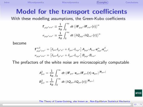
Model for the transport coefficientsWith these modelling assumptions, the Green-Kubo coefficients
Γµµ′νν′ ≡1
kB
∫ ∞
0dt⟨
δFµµ′ δFνν′ (t)⟩α
κµµ′νν′ ≡1
kB
∫ ∞
0dt⟨
δQµµ′ δQνν′ (t)⟩α
become
Γαβµµ′νν′
=[
δµνδµ′ν′ + δµν′ δνµ′
]
Aµµ′Aνν′eαµµ′eβνν′
κµµ′νν′ =[
δµνδµ′ν′ + δµν′ δνµ′
]
Bµµ′Bνν′
69 / 74
The Theory of Coarse-Graining, also known as , Non-Equilibrium Statistical Mechanics

Intro Microdynamics Macrodynamics Examples Conclusions
Model for the transport coefficientsWith these modelling assumptions, the Green-Kubo coefficients
Γµµ′νν′ ≡1
kB
∫ ∞
0dt⟨
δFµµ′ δFνν′ (t)⟩α
κµµ′νν′ ≡1
kB
∫ ∞
0dt⟨
δQµµ′ δQνν′ (t)⟩α
become
Γαβµµ′νν′
=[
δµνδµ′ν′ + δµν′ δνµ′
]
Aµµ′Aνν′eαµµ′eβνν′
κµµ′νν′ =[
δµνδµ′ν′ + δµν′ δνµ′
]
Bµµ′Bνν′
The prefactors of the white noise are microscopically computable
A2µν =
1
kB
∫ ∞
0dt 〈δFµν ·eµνδFµν(t)·eµν 〉
RPE
B2µν =
1
kB
∫ ∞
0dt 〈δQµνδQµν(t)〉
RPE
69 / 74
The Theory of Coarse-Graining, also known as , Non-Equilibrium Statistical Mechanics
Intro Microdynamics Macrodynamics Examples Conclusions
Model for the transport coefficientsWith these modelling assumptions, the Green-Kubo coefficients
Γµµ′νν′ ≡1
kB
∫ ∞
0dt⟨
δFµµ′ δFνν′ (t)⟩α
κµµ′νν′ ≡1
kB
∫ ∞
0dt⟨
δQµµ′ δQνν′ (t)⟩α
become
Γαβµµ′νν′
=[
δµνδµ′ν′ + δµν′ δνµ′
]
Aµµ′Aνν′eαµµ′eβνν′
κµµ′νν′ =[
δµνδµ′ν′ + δµν′ δνµ′
]
Bµµ′Bνν′
The prefactors of the white noise are microscopically computable
A2µν =
1
kB
∫ ∞
0dt 〈δFµν ·eµνδFµν(t)·eµν〉
|Rµν |
B2µν =
1
kB
∫ ∞
0dt 〈δQµνδQµν (t)〉
|Rµν |
69 / 74
The Theory of Coarse-Graining, also known as , Non-Equilibrium Statistical Mechanics

Intro Microdynamics Macrodynamics Examples Conclusions
The simpler SDE
Under the approximations on the transport coefficients we have
Rµ = Vµ
Pµ =M∑
ν
〈Fµν〉RE−
M∑
ν
γµν(eµν ·Vµν)eµν +∑
ν
Fµν
Eµ = −1
2
M∑
ν
〈Fµν〉RE ·Vµν+
M∑
ν
κµν
[
1
Tµ−
1
Tν
]
+M∑
ν
γµν(Vµν ·eµν)2
+M∑
ν
[
Qµν − Vµν ·Fµν
]
These are the equations of DPD+E (Espanol ’97, Bonet &
Mackie ’97) BUT with microscopic foundation.
70 / 74
The Theory of Coarse-Graining, also known as , Non-Equilibrium Statistical Mechanics

Conclusions

Intro Microdynamics Macrodynamics Examples Conclusions
Conclusions
The Theory of Coarse-Graining gives the dynamics of CGvariables.
72 / 74
The Theory of Coarse-Graining, also known as , Non-Equilibrium Statistical Mechanics

Intro Microdynamics Macrodynamics Examples Conclusions
Conclusions
The Theory of Coarse-Graining gives the dynamics of CGvariables.
Another name for it is Non-Equilibrium Statistical Mechanics.
72 / 74
The Theory of Coarse-Graining, also known as , Non-Equilibrium Statistical Mechanics

Intro Microdynamics Macrodynamics Examples Conclusions
Conclusions
The Theory of Coarse-Graining gives the dynamics of CGvariables.
Another name for it is Non-Equilibrium Statistical Mechanics.
Black-Box: The derivation of the dynamic equations is just arecipe.
The structure of the equations is determined by iLA(z).
The essential assumption is the separation of time scales orMarkov property.
Markov allows you to run short MD simulation to extractmacroscopic parameters.
72 / 74
The Theory of Coarse-Graining, also known as , Non-Equilibrium Statistical Mechanics

Intro Microdynamics Macrodynamics Examples Conclusions
The big problems of the theory of CG
You need to know in advance what are the CG variables.
73 / 74
The Theory of Coarse-Graining, also known as , Non-Equilibrium Statistical Mechanics

Intro Microdynamics Macrodynamics Examples Conclusions
The big problems of the theory of CG
You need to know in advance what are the CG variables.
These variables should be slow (Markovian).
73 / 74
The Theory of Coarse-Graining, also known as , Non-Equilibrium Statistical Mechanics

Intro Microdynamics Macrodynamics Examples Conclusions
The big problems of the theory of CG
You need to know in advance what are the CG variables.
These variables should be slow (Markovian).
The Curse of Dimensionality: Drift and Diffusion dependon all the CG variables.
The theory gives you the structure of the equations.
73 / 74
The Theory of Coarse-Graining, also known as , Non-Equilibrium Statistical Mechanics
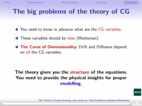
Intro Microdynamics Macrodynamics Examples Conclusions
The big problems of the theory of CG
You need to know in advance what are the CG variables.
These variables should be slow (Markovian).
The Curse of Dimensionality: Drift and Diffusion dependon all the CG variables.
The theory gives you the structure of the equations.You need to provide the physical insights for proper
modelling.
73 / 74
The Theory of Coarse-Graining, also known as , Non-Equilibrium Statistical Mechanics


![STOCK: Structure Mapper and Online …praprot/publications/Bevc_et_al-2015...STOCK: Structure Mapper and Online Coarse-Graining Kit for Molecular Simulations Stas Bevc,*[a] Christoph](https://static.fdocuments.in/doc/165x107/5ad037757f8b9a56098e197b/stock-structure-mapper-and-online-praprotpublicationsbevcetal-2015stock.jpg)