NUMERICAL ANALYSIS OF ANCHORED CONCRETE PILE WALL:

A CASE STUDY

A MASTER’S THESIS

in

Civil Engineering

Atılım University

by

KIVANÇ SİNCİL

SEPTEMBER 2006

NUMERICAL ANALYSIS OF ANCHORED CONCRETE PILE WALL:

A CASE STUDY

A THESIS SUBMITTED TO

THE GRADUATE SCHOOL OF NATURAL AND APPLIED SCIENCES

OF

ATILIM UNIVERSITY

BY

KIVANÇ SİNCİL

IN PARTIAL FULFILLMENT OF THE REQUIREMENTS FOR THE DEGREE OF

MASTER OF SCIENCE

IN

THE DEPARTMENT OF CIVIL ENGINEERING

SEPTEMBER 2006

Approval of the Graduate School of Natural and Applied Sciences

_____________________

Prof. Dr. Selçuk Soyupak

Director

I certify that this thesis satisfies all the requirements as a thesis for the degree of Master of Science.

_____________________

Prof. Dr. Erol Uluğ

Head of Department

This is to certify that we have read this thesis and that in our opinion it is fully adequate, in scope and quality, as a thesis for the degree of Master of Science.

_____________________

Dr. Y. Dursun Sarı

Supervisor

Examining Committee Members

Dr. B. Sadık Bakır _____________________

Dr. M. Serdar Nalçakan _____________________

Dr. Y. Dursun Sarı _____________________

iii

ABSTRACT

NUMERICAL ANALYSIS OF ANCHORED CONCRETE PILE WALL:

A CASE STUDY

Sincil, Kıvanç

M.S., Civil Engineering Department

Supervisor: Dr. Y. Dursun Sarı

September 2006, 109 pages

This thesis reviews the numerical analysis of anchored concrete pile walls

and comparison of field measurements and numerical values in terms of the stability

of the structure and soil. The deep excavation supported by anchored pile walls,

namely Gazino Station excavation, Ulus-Keçiören Metro project. After an extensive

literature review on anchors, anchored structures and deep excavations, the

excavation of Gazino Station is described and modelled and analyzed by FEM

program Plaxis. Special emphasis was given to selection of soil parameters for

numerical analysis, since these parameters play a key role in the success of the

analysis.

The numerical analysis results tend to overestimate the measured lateral

wall deflections above the excavation level, the numerical analysis proves to be quite

satisfactory for considering the preliminary analysis of the concrete pile wall with

and without anchorage. The results can be accurate if more extensive and attentive

field and laboratory will be carried out together with numerical modeling.

Keywords: Numerical Analysis, Anchor, Pile Wall, Lateral Wall Deflection, Lateral

Earth Pressure, Settlement

iv

ÖZ

ANKRAJLI KAZIK DUVARLARIN SAYISAL ÇÖZÜMLENMESİ:

DURUM ANALİZİ

Sincil, Kıvanç

Yüksek Lisans, İnşaat Mühendisliği Bölümü

Tez Yöneticisi: Dr. Y. Dursun Sarı

Eylül 2006, 109 sayfa

Bu tez, ankrajlı kazık duvarların sayısal analizi ile yerinde ölçümler ile

sayısal verilerin, üst yapı ve zemin stabilitesi açısından karşılaştırılmasını

içermektedir. Ulus-Keçiören Metro projesi çalışmaları kapsamında, Gazino İstasyonu

derin kazısı ankrajlı kazık duvarlar ile desteklenmiştir. Ankrajlar, ankrajlı yapılar ve

derin kazılar ile ilgili detaylı bir literatür taramasının ardından, bahsedilen Gazino

İstasyonu kazısı, Plaxis isimli bir sonlu elemanlar programı kullanılarak modellenmiş

ve analiz edilmiştir. Sayısal analizde kullanılacak olan zemin parametreleri yöntemin

başarısında anahtar rol oynadığından, bu parametrelerin seçimine önem verilmiştir.

Sayısal analiz sonuçları kazı seviyesinin üstündeki yatay duvar

deplasmanlarını ölçülenden daha büyük, kazı seviyesinin altındaki deplasmanları ise

ölçülenlerden daha küçük bulma olasılığına rağmen, saha ölçümlerindeki dağılım ve

güvenilirlilik dikkate alındığında sayısal analiz sonuçları tatminkar olarak

değerlendirilmiştir. Zemin parametrelerinin seçiminde yardımcı olacak daha detaylı

ve özenli saha ve laboratuvar deneyleri sayısal modellemelerle desteklendiğinde

sonuçlar daha doğru ve geçerli olacaktır.

Anahtar Kelimeler : Sayısal Analiz, Ankraj, Kazık, Kazık Yanal Yerdeğiştirmesi,

Yanal Zemin Basıncı, Oturma

v

ACKNOWLEDGMENTS

I express sincere appreciation to my supervisor Dr. Y. Dursun Sarı for his guidance

and insight throughout the research. Thanks also to Murat Çilsal and for his

technical assistance.

I would also like to thank to Dr. Sadık Bakır and Dr. M. Serdar Nalçakan for their

support, encouragement, insight and guidance during this study.

To my family and friends for their technical assistance, and for their continuous

support and patience during this period.

vi

TABLE OF CONTENTS

ABSTRACT iii

ÖZ iv

ACKNOWLEDEGMENTS v

TABLE OF CONTENTS vi

LIST OF TABLES ix

LIST OF FIGURES xi

LIST OF ABBREVIATIONS xv

CHAPTER

1. INTRODUCTION....................................................................................... 1

1.1.Statement of the Problem................................................................. 3

1.2.Scope and Outline of the Thesis...................................................... 4

2. BACKGROUND INFORMATION AND LITERATURE SURVEY........ 6

2.1.Ground Anchors............................................................................... 6

2.1.1. The Terminology......................................................... 9

2.1.2. Anchors in Sands......... ............................................... 11

2.1.3. Anchors in Stiff Clays................................................. 12

2.2. Fundamentals of Anchored Walls.................................................. 16

2.2.1. Working Principles..................................................... 16

2.3. Anchor – Wall Characteristics and Applicability............................... 16

2.3.1. Anchored Sheet Pile Walls..........................................16

2.3.2. Anchored Soldier Pile Walls....................................... 17

2.4. Examples of Anchored Walls......................................................... 18

2.5. Estimation of Lateral Stresses and Deformations of Piles.....................22

2.5.1. General Requirements................................................ 22

2.5.2. Initial Stresses............................................................. 22

2.5.3. Constitutive Equations................................................ 23

2.5.4. Boundary Conditions.................................................. 23

2.6. Lateral Earth Pressure.................................................................... 24

2.7. Active and Passive Earth Pressures................................................ 25

2.8. Coefficient of Earth Pressure......................................................... 26

vii

2.9. The Rankine Theory....................................................................... 27

2.10. The Coulomb Theory ……………………………………………. 28

2.11. Earth Pressure Coefficient when At-Rest...................................... 29

2.12. Wall Friction.................................................................................. 30

2.13. Elastic Analysis.............................................................................. 30

2.13.1. Linear Analysis........................................................... 31

2.14. Analysis of Anchored Walls by Finite-Element Methods……………. 35

2.14.1. Advantages and Limitations....................................... 35

2.14.2. Statement of a Model.................................................. 35

2.14.3. Examples of Finite Element Analysis......................... 36

3. FIELD STUDIES...... .................................................................................. 50

3.1. Geological Studies......................................................................... 51

3.2. Laboratory Studies......................................................................... 52

3.3. Geotechnical Evaluation................................................................ 54

3.3.1. General Geology......................................................... 54

3.3.2. Local Geology............................................................. 55

4. MODELLING OF GAZİNO STATION ANCHORED PILE WALL........58

4.1. Layout Plan of Gazino Station....................................................... 58

4.2. Prediction of Soil and Rock Properties of the Model.................... 60

4.3. Geometry Model............................................................................ 73

4.4. Material properties of the Model.................................................. 74

4.5. Mesh Generation of the Model...................................................... 79

4.6. K0 Procedure in Plaxis................................................................... 81

4.7. Calculations.................................................................................... 83

4.7.1. Required Results......................................................... 83

4.7.2. Case Studies................................................................ 83

4.7.3. Model Results.............................................................. 84

4.7.3.1.Pile Wal Laterall Displacements............... 84

4.7.4. Stress – Strain Relation.............................................. 86

4.7.4.1.Mohr – Coulomb Model............................. 86

4.7.5. Settlements at the surface behind pile wall…………... 95

4.7.6. Anchor Forces……………………………………….. 96

4.7.7. Safety Analysis……………………………………….. 97

viii

4.7.8. Active & Passive Earth Pressures…………………… 99

4.7.9. Heave of the Soil in front of the Wall………………… 101

5. RESULTS & DISCUSSION…………………………………….................. 102

5.1. Lateral Deflection of Pile Wall...................................................... 102

5.2. Stress – Strain Behavior................................................................. 102

5.2.1. Non-Anchored Behavior……………………………... 102

5.2.2. Anchored Behavior…………………………………... 103

6. CONCLUSION............................................................................................104

REFERENCES............................................................................................ 107

ix

LIST OF TABLES

TABLE

2.1. Typical Flowchart and Procedure Leading to Finite-Element Analysis……..... 36

3.1. Boring Logs and Depths at the Subway Route……………........................... 51

3.2. Jetting Water Test Results for Gazino Station ……………………………... 53

3.3. Soil Mechanics Laboratory Test Results…………………………………… 53

3.4. Weight per Unit Volume (γ) and Uniaxial Compressive Strength (UCS) Test Results……………………………………………………………..........70 4.1. Consistency of clays and approximate correlation to the standard penetration number, N (Das, 1984)…………………………………………...63

4.2. Typical ground parameters (Carter&Bentley, 1991)…………………………... 63

4.3. Soil classification and CPT-SPT correlations (Lunne, Robertson&Powell, 1997)…... 66

4.4. Estimation of constrained modulus, M, for clays (Lunne,Robertson%Powell,1997)……………………………………………. 67

4.5. Empirical values for φ, Dr, and unit weight of granular soils based on the SPT at about 6 m depth and normally consolidated (Bowles, 1988)...................... 70 4.6 Relation between N-values, relative density, and angle of friction in sands (Das, 1984)..................................................................................................... 70 4.7. Soil and interface properties………………………………………………….. 75 4.8. Properties of the pile (beam)………………………………………………….75

4.9. Properties of the pile cap (beam)…………………………………………........ 75

4.10. Properties of the anchor rod (node-to-node anchors)………………………..78

4.11. Property of the grout body (geotextile)…………………………………….. 78

x

4.12. Stress-Strain Values foe selected points at each case…..…………………… 90

4.13. Anchor Forces………………………………………………………………... 96

4.14.... ΣMsf values for Gazino Station at excavation stages……………………. 98

4.15. Comparison of FEM and Rankine Results………………………………… 100

xi

LIST OF FIGURES

FIGURES

2.1. Schematic presentation of a ground anchor showing the three main

components (Xanthakos, 1991)................................................................... 7

2.2. Ground anchor use for retaining wall support (Hanna, 1982)Use of ground

anchors for rock slope stabilization (Hanna, 1982)..................................... 7

2.3. Ground Anchors (a) grouted mass formed by pressure injection,

(b) grout cylinder, (c) multiple under-reamed anchor …………………… 12

2.4. Use of ground anchors for rock slope stabilization (Hanna, 1982)………. 14

2.5. Cheurfas Dam in Algeria: a) general plan; b) section through main structure

showing the anchorage.(Xanthakos, 1991)……………………………….. 15 2.6. Excavation for subway construction in Munich; inclined bored pile wall

strutted at the top and anchored in the lower levels. (Littlejohn, 1982)... 18

2.7. Typical section, deep excavation for building in Stockholm

(Littlejohn, 1982)……..…………………………………………………... 19

2.8. Protection of excavation from groundwater and uplift by lowering

the water table permanently within the excavation area …………………. 20

2.9. Roche Building; typical cross section for the basement excavation.

(Fenoux, 1971)…………………………………………………………….21

xii

2.10. Active and Passive Zone.............................................................................. 26

2.11. Active Earth Pressure – Angular Parameters ……………………….……. 27

2.12. Lateral pressure distribution for different boundary conditions, wall,

condition of no lateral yield (Morgenstern and Eisenstein, 1970)………. 32

2.13. Lateral pressure distribution for different boundary conditions, wall of

Fig2.12; pressure diagrams for wall yielding 0.0025H towards active state.

(Morgenstern and Eisenstein, 1970)……………………………………… 34

2.14. Anchored wall in clay; (a) section through wall;

(b) soil data and prestressed diagram. (Tsui, 1973)……………………… 37

2.15. Construction sequence; Finite element analysis of the anchored wall of

Fig.2.14 (Tsui, 1973)……………………………………………………... 38

2.16. Detail Wall and ground movements predicted by finite-element analysis; tied-

back wall of Fig2.14. (Tsui, 1973)………………………………………... 39

2.17. Lateral earth pressure predicted by finite-element analysis, and appearance

pressure diagrams, tied-back wall of Fig.2.14. (Tsui, 1973)…………....... 39

2.18. Lateral earth pressure behind a flexible wall predicted by finite-element

analysis; prestressed tied- back wall. (Clough and Tsui, 1974)…………... 40

2.19. Plan of site showing layout of anchored wall

(Barla and Mascardi, 1974)……………………………………………… 41

2.20. Vertical section along anchored retaining wall showing various stages of

excavation (After Barla and Mascardi, 1974)……………………………. 42

xiii

2.21. Vertical cross-section through the anchored wall

(After Barla and Mascardi, 1974)………………………………….……... 43

2.22. Anchored diaphragm wall for CPF building, Singapore

(After Littlejohn and MacFarlane, 1974)………………………………….. 43

2.23. Arrangement of ground anchors to support deep Excavation for Subway

Station in Munich (After Ostermayer, 1974)............................................... 44

2.24. Cross Section……………………………………………………………... 46

2.25. Measured and predicted behavior of Section A-A walls early stages of

excavation................................................................................................... 47

2.26. Measured and predicted behavior of Section B-B walls early stages of

excavation.................................................................................................... 48

2.27. Shear stress-strain behavior of Hardening Soil (HS) model

(Schanz et al., 1999)………………………………………........................ 49

3.1 The route of Ulus-Keçiören Metro Project.................................................. 50

3.2 Main geological map of Ankara.................................................................. 54

3.3 General Geology of Gazino Station............................................................. 57

4.1 Plan view of Gazino Station........................................................................ 59

4.2 A-A’ section view of the Gazino Station................................................... 60

4.3 Drilling Log Sheet SPT and Pressuremeter Test Results............................. 62

xiv

4.4 Relationships between angle of shearing resistance and plasticity index

(Carter&Bentley, 1991)..................................................................................64

4.5 Correlation between angle of shearing resistance and plasticity index for

normally consolidated clays (Bowles, 1988)................................................. 65

4.6 The variation of f2 = 1/mv with plasticity index (Stroud, 1974)..................... 65

4.7. Plot of standard penetration resistance vs. angle of friction for granular

soils (Das, 1983)………………………………………………………….71

4.8. Correlation of standard penetration resistance (NAVFAC DM-7.1)........... 72

4.9. Modeled Section.......................................................................................... 74

4.10. Position of nodes and stress points in a 3-node beam element……………… 76

4.11. Plaxis Model………………………………………………………………... 79

4.12. FEM Results of Pile Wall lateral deflection for each excavation stage…….. 85

4.13. Comparison of Pile Cap lateral displacement with and without anchors…… 86

4.14. Engineering Stress-Strain Curve…………………………………………… 87

4.15. τ - σ graph and Mohr-Coulomb Failure Envelope as σh’ increasing……... 87

4.16. Plastic points occured after Case 3.............................................................. 88

4.17. Selected Stress-Points for Stress-Strain Values........................................... 89

4.18. Stress-Strain behavior of the clusters (after case 3)..................................... 91

4.19. Plastic Points occured after case 6............................................................... 92

4.20. Comparison of stress-strain relation of fill layer

with and without anchors............................................................................. 93

4.21. Principal effective stresses at the final stage (Case 6)……………………… 95

4.22. The subsidence at point J…………………………………………………... 95

4.23. Active and Passive thrusts on the wall…………………………………….. 99

4.24. Rankine and FEM result for active and passive earth pressure distribution.. 100

4.25. Computed Heave in front of the Wall……………………………………… 101

xv

LIST OF ABBREVIATIONS

A Ratio of normal pressure at interface to effective overburden pressure B Bearing capacity factor,

Be Width of Excavation BS British Standards

Ca Shaft Adhesion Cu Shear Strength Cub Undrained shear strength at proximal end of fixed anchor

c Effective cohesive strength(Cohesion)

D Diameter of fixed anchor

d Diameter of borehole

Dr Relative Density DIN Deutsches Institut für Normung

E Young’s Modulus of Elasticity

EA Normal Stiffness

EI Bending Stifness

xvi

Ed Drained Young’s Modulus of Elasticity

G Elastic Shear Modulus

h Depth of overburden Ic Consistency Index ISRM International Society for Rock Mechanics

Ko Coefficient of lateral pressure at rest

KA Coefficient of lateral pressure at active state KP Coefficient of lateral pressure at passive state L Fixed anchor length LL Liquid Limit l Length of Shaft m Natural Moisture Content

mv Coefficient of volume of compressibility

Nc Bearing capacity factor

OCR Overconsolidation Ratio

PL Plastic Limit PI Plasticitiy Index PH Lateral Earth Pressure Pv Vertical Earth Pressure Qf Ultimate load capacity of anchor Qult Ultimate bond or skin friction at rock/grout interface

xvii

qc Measured cone resisitance

SPT, N Standard penetration number

USC Unitied Soil Classification

W Weight per unit volume

α Skin friction coefficient β Embankment Level γ The unit weight of soil

ε Strain

δhmax Maximum lateral wall displacement δvmax Maximum vertical wall displacement(Settlement)

φ' Angle of shearing resistance for effective stress

φ Internal Friction Angle of the Soil

σ Mohr-Coulomb Principle Stress of the Soil

τf Shear Strength of the Soil

τM Skin Friction

δ Wall Friction

ν Poisson's Ratio

ψ Angle of dialatancy

1

CHAPTER I

INTRODUCTION

Anchor piles and ground anchors have been used in civil works for a long period of

time and a considerable amount of technical study have been performed and these

studies revealed significant technical knowledge and construction expertise. The

digging of an excavation in the ground causes stress changes in the ground. These

stress changes indicates a variety in the stress distribution particularly around the

excavation. These stress changes caused by the roof and wall pressures due to the

excavation bring out the displacements around the excavation which can cause the

deformations and loosening of soil especially on the surface of the slope, retaining

walls and cliff walls. One of the most important cases is to control these

displacements and deformations with the help of some excavation supports. The

greatest use of prestressed anchors with piles is in the support of both temporary and

permanent excavations.

The main purpose in an excavation is to help rock to support itself. The subject of

piling and ground anchoring can be considered in some details and one of the

important subjects is the displacement of the anchor piles due to the excavation and

by applying anchorage the deformations and soil movements can be kept under

control. Load-deformation behavior of anchor piles and anchors is a straightforward

topic to discuss but also a general look to examine in detail some various factors. The

performance of an anchored structure depends on how the anchor develops load.

Another important case is the load testing of anchors to understand the behavior of

the anchors in different types of rock and soil. In another words load testing is the

accepted method for checking the performance and suitability of anchors. Within the

load testing procedures there are interrelated factors to be considered which are the

anchor materials, the ground itself and stressing equipment. There are also suggested

methods for anchorage testing which have to be considered during the test

procedures. For an anchor to function, it has to be displaced relative to the medium in

2

which it is installed. However, it does not have to be prestressed and there are many

instances where non-prestressed anchors or tension piles are used.

While following a suggested method for anchorage testing there are also certain

parameters to consider which are; fixed anchor length, free anchor length, fixed

anchor diameter, shaft diameter, shaft length, etc. also the parts of the anchor that are

interacted with the ground.

The method of anchor stressing is usually by direct pull from a hydraulic jack. A

torque wrench is occasionally used. Details of stressing and the suggested methods

are clearly defined by ISRM: Rock Anchorage Testing. Some useful guidance is also

given by Littlejohn&Bruce (1976).

Today there are some forms of anchor test in use and useful general guidance on

such tests is given by Ostermayer (1974, 1976) and DIN 4125. There are also many

other guidance on such tests and they all have some recommendations for ground

anchors testing. (DIN, BS, S1A 191, French Code, German Code, Bureau Securitas,

etc.)

There are also some other ground exploration and site investigations are needed

which are required before designing the anchored structure. The general geology of

the site and the topographical features affect the design and construction. Details of

the various soil and rock strata and ground water tables may affect the anchorage

during construction. By means of some laboratory tests on the soil and rock samples,

in-situ tests, soil and rock mechanics investigations will also help to select the proper

anchorage.

Today a large number of stabilization methods are available. Within this study the

behavior of the anchor pile wall is investigated and a FEM analysis is carried out.

The design methods are also considered but no attempt has been made to describe

design methods. The main objective is to investigate the anchored pile wall behaviors

and to expose some reasonable result parameters for the subway station construction

according to a failure criterion (Mohr-Coulomb) and Rankine’s Active&Passive

earth pressure theory. Geological and design parameters and considerations, the

3

observed anchored pile wall behaviors, anchor prestress results are obtained from the

designer and consultant and the study is performed by constituting a theoretical

model and this model is incorporated into a Windows based program called Plaxis.

Plaxis has been used to investigate pile wall behaviors, stabilization and a FEM

analysis of the study with the design considerations and field observations.

1.1. Statement of the Problem

When the ground is excavated the main matter is the stabilization of the walls around

the opening in case of the stability of the superstructure and the other structures

which are constructed before. (e.g. buildings next to the cliff walls, motorways above

a tunnel, etc.)

There are also some natural effects which can always present instability problems

and have to be considered before the stabilization study. The most important

considerations are quantification of the ground material, particularly joints and

fissures, understanding of the water pressures, weathered or unweathered rock

conditions, landslide and earthquake conditions, etc. A detailed geological study is

also required to figure out these parameters and to make a decision about the

stabilization method of the ground. When the effect of the stabilization is considered

the study about the stabilization method becomes more important to determine the

optimum design, construction and cost studies.

There are many stabilization methods available in civil and mining constructions.

The most used excavation supports are rock bolts and ground anchorages. There are

also many types of bolt and anchor types and during this study some of the anchor

types will be mentioned and as pointed out previously the anchor piles will be

considered and the behavior of the anchored pile and excavation walls will be

investigated in the scope of stabilization. The study will make progress within the

field studies, observations and numerical analysis study results.

4

To determine the parameters of the soil due to the Mohr-Coulomb criteria during

excavation and to study the interaction of these parameters is very important to

estimate the problems which can occur during the excavation like landslide, slope or

failure increase of strain, etc. During the construction of the anchor piles and anchors

these parameters have to be studied carefully and one of the most important subjects

is the anchor arrangement and spacing of anchors which can cause failures that are

mentioned above unless it is designed and constructed properly.

1.2. Scope and Outline of the Thesis

Investigation of the stabilization problems that are mentioned above is possible with

the determination of the design parameters and interaction of the parameters which

effects the deformations into the ground during the excavation and stabilization

studies.

In this study the displacements of the anchored pile wall is investigated which are

constructed at the Gazino Station for the stabilization of the excavation. The

deformations into the ground and the anchorage method and testing procedures are

studied and investigated to bring up a conclusion. The anchorages are applied for the

stabilization after the piles are constructed and the constructing of anchor rows and

testing procedures were still on process.

No stabilization problems encountered during the construction of Gazino Station but

the unpredicted deformations and displacements on the pile walls and on the cap of

piles may occur and these cause unforeseen circumstances on the walls and in the

support of permanent excavation.

The data and parameters which are obtained from the field studies will be evaluated

in all manner of how are the deformations effects. Thus by using the whole field data

and study results the probable but unpredictable anchor and ground failures can be

estimated.

5

In this study which the anchor type, anchor arrangement, pile designs, geological

considerations, field and laboratory studies, anchor testing procedures are predicted

and certain, the main objective is to investigate the anchored pile wall stability and

evaluation of the behavior by using the Mohr-Coulomb and Rankine theory. A FEM

analysis and an evaluation of field measurements are considered in the manner of the

stabilization of the deep excavation.

In the first chapter, the problem is defined and a scope of the thesis is described.

Chapter Two gives the background information and some literature survey about the

anchored pile wall applications and there are also some definitions given in this

chapter.

Chapter Three describes the field studies performed within the study of Metro

Project and some test results are also given.

Chapter Four gives the modeling and calculation results and some brief explanations

about the calculation results.

Chapter Five gives discussion of the results.

Finally, conclusions derived from this study and the recommendations for further

studies are provided in Chapter Six.

6

CHAPTER II

BACKGROUND INFORMATION AND LITERATURE SURVEY

2.1. Ground Anchors

A ground anchor normally consists of a high tensile steel cable or bar, called the

tendon, one end of which is held securely in the soil by a mass of cement grout or

grouted soil: the other end of the tendon is anchored against a bearing plate on the

structural unit to be supported. The main application of ground anchors is in the

construction of tie-backs for diaphragm or pile walls. Other applications are in the

anchoring of structures subjected to overturning, sliding or buoyancy, in the

provision of reaction for in-situ load tests and in pre-loading to reduce settlement.

Ground anchors can be constructed in sands (including gravelly sands and silty

sands) and stiff clays, and they can be used in situations where either temporary or

permanent support is required (Craig R.F. , 1978).

Anchors transmit tensile forces into the rock mass. They are inserted into boreholes

and bonded to the rock by grout or other chemicals. Their action is twofold. Firstly,

on tensioning an anchor or rock bolt, the stress field is modified in the vicinity of the

anchor. Secondly, where a tensioned anchor is holding a block of rock in its original

position it also acts as a preventative measure against the further disintegration of the

rock.

A ground anchor functions as load carrying element, consisting essentially of a steel

tendon inserted into suitable ground formations in almost any direction. Its load-

carrying capacity is generated as resisting reaction mobilized by stressing the ground

along a specially formed anchorage zone. (Xanthakos, 1991)

This arrangement is shown schematically in Fig.2.1 together with the basic

components of the system. These components include the head, the free length, and

the bond length. The latter is intended to interact with the enveloping ground

7

materials in order to transfer the load; whereas the free length remains unbonded and

thus free to move within the soil environment.

Fig.2.1

Schematic presentation of a ground anchor showing the three main components (Xanthakos, 1991)

Fig.2.2

Ground anchor use for retaining wall support (Hanna, 1982)

8

As structural devices, anchors usually are attached to ground supports at their head.

The anchor tendon is installed in special boreholes in a wide variety of soils or rock.

The grouted length of tendon, through which force is transmitted to the surrounding

soil, is called the fixed anchor length. The length of tendon between the fixed anchor

and the bearing plate is called the free anchor length: no force is transmitted to the

soil over this length. For temporary anchors the tendon is normally greased and

covered with plastic tape over the free anchor length. This allows for free movement

of the tendon and gives protection against corrosion. For permanent anchors the

tendon is normally greased and sheathed with polythene under factory conditions: on

site the tendon is stripped and de-greased over what will be the fixed anchor length.

The ultimate load which can be carried by an anchor depends on the soil resistance

(principally skin friction) mobilised adjacent to the fixed anchor length. (This, of

course, assumes that there will be no prior failure at the grout-tendon interface or of

the tendon itself). Anchors are usually prestressed in order to reduce the movement

required to mobilise the soil resistance. Each anchor is subjected to a test loading

after installation: temporary anchors are usually tested to 1-2 times the working load

and permanent anchors to 1-5 times the working load. Finally, prestressing of the

anchor takes place. Creep displacements under constant load will occur in ground

anchors. A creep coefficient, defined as the displacement per unit log time, can be

determined by means of a load test. It has been suggested that this coefficient should

not exceed 1 mm for 1-5 times the working load.

A comprehensive ground investigation is essential in any location where ground

anchors are to be employed. The soil profile must be determined accurately, any

variations in the level and thickness of strata being particularly important. In the case

of sands the particle size distribution should be determined, in order that permeability

and grout acceptability can be estimated. The relative density of sands is also

required to allow an estimate of φ to be made. In the case of stiff clays the undrained

shear strength should be determined.

9

2.1.1. The Terminology

Within this chapter some special terms are defined and a brief explanation for each

term is given by Hobst&Zajic.

The anchoring of structures to rock or soil ensures their mutual interconnection. This

interconnection, which is capable of transferring tensile and shear forces, solely

dependent on the use of anchors, a system of which forms the total anchorage.

An anchor is a device with a static function, transferring forces in a given direction

from the structure to the rock or soil.

The anchor head is situated at the external end of the anchor; from it the prestressing

of the anchor is carried out, and when connected it transmits the anchoring forces to

the structure.

The anchor tendon connects the anchor head with the root. The tendon usually

allows, by virtue of its elastic deformation, the prestressing of the anchor during

anchoring.

The anchor root is situated at the subterranean end of the anchor, and transfers the

tensile forces from the tendon to the ground. The root must be adequately fixed in the

ground for this purpose.

The free length of an anchor (tendon) is determined by the distance between the

starting point of the fixing of the tendon in the anchor root, and the fixing point of

the tendon in the anchor head.

The fixed portion (root) of the anchor in the rock or soil is determined by the length

along which the force within the anchor is transferred to the ground.

A temporary anchor has a service life not exceeding two years.

A permanent anchor has a service life more than two years.

10

A prestressed anchor is permanently tensioned due to the elastic extension of the

tendon over its free length.

A non-prestressed anchor is one that is left without prestressing, or one that cannot in

any case be prestressed because it is fixed in the ground along its entire length.

The prestressing of an anchor is a process in which a tensile force is introduced.

The anchoring force is the force which is transmitted by the anchor to the ground.

The working load of an anchor is the force which the anchor should be capable of

transmitting continuously throughout its service life.

The admissible load of an anchor is determined by the upper limit of its bearing

capacity, computed or ascertained during tests with subtraction of a safety margin.

A testing load is a short-term loading to which the test anchor is subjected in order to

check the quality of its manufacture and establish its maximum load.

The (limit) bearing capacity of an anchor is that load under which the resistance of

any functional part of the system (ground, anchor, anchored structure) fails and the

anchor ceases to function.

The safety factor is the ratio of the limit load or limit deformation load of the anchor

and of its admissible or working load.

11

2.1.2. Anchors in Sands

In general the sequence of construction is as follows. A cased borehole (diameter

usually within the range 75 – 125 mm) is advanced through the soil to the required

depth. The tendon is then positioned in the hole and cement grout is injected under

pressure over the fixed anchor length as the casing is withdrawn. The grout

penetrates the soil around the borehole, to an extent depending on the permeability of

the soil and on the injection pressure, forming a zone of grouted soil, the diameter of

which can be up to four times that of the borehole (Fig.2.3a). Care must be taken to

ensure that the injection pressure does not exceed the overburden pressure of the soil

above the anchor, otherwise heaving of fissuring may result. When the grout has

achieved adequate strength the other end of the tendon is anchored against the

bearing plate. The space between the sheathed tendon and the sides of the borehole,

over the free anchor length, is normally filled with grout (under low pressure): this

grout gives additional corrosion protection to the tendon.

The ultimate resistance of an anchor to pull-out is equal to the sum of the side

resistance and the end resistance of the grouted mass. The following theoretical

expression was proposed by Littlejohn:

( )

−+

+= 22

4tan

2dD

hBDL

LhAQ f γφπγ (2.1)

where

Qf : ultimate load capacity of anchor, [kN] A : ratio of normal pressure at interface

to effective overburden pressure, [-] γ : unit weight of soil [kN/m3] B : bearing capacity factor, [-] h : depth of overburden, [m] L : fixed anchor length, [m] D : diameter of fixed anchor, [m] d : diameter of borehole [m]

12

Fig2.3

Ground Anchors (a) grouted mass formed by pressure injection, (b) grout cylinder, (c) multiple under-reamed anchor.

It was suggested that the value of A is normally within the range 1 to 2. The factor B

is analogous to the bearing capacity factor Nq in the case of piles and it was

suggested that the ratio Nq/B is within the range 1-3 to 1-4, using the Nq values of

Berezantzev, Khristoforov and Golubkov. However, the above expression is unlikely

to represent all the relevant factors in a complex problem.

The ultimate resistance also depends on details of the installation technique and a

number of empirical formulae have been proposed by specialist contractors, suitable

for use with their particular technique.

2.1.3. Anchors in Stiff Clays

The simplest construction technique for anchors in stiff clays is to auger a hole to the

required depth, position the tendon and grout the fixed anchor length using a tremie

pipe (Fig.2.3b). However, such a technique would produce an anchor of relatively

low capacity because the skin friction at the grout-clay interface would be unlikely to

exceed 0,3Cu (i.e. α=0,3). (Cu : shear strength, α: side resistance(skin friction

coefficient))

13

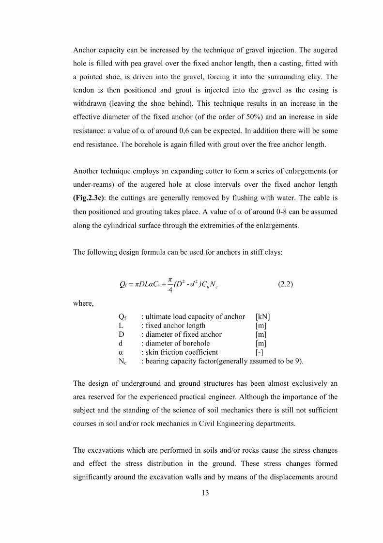
Anchor capacity can be increased by the technique of gravel injection. The augered

hole is filled with pea gravel over the fixed anchor length, then a casting, fitted with

a pointed shoe, is driven into the gravel, forcing it into the surrounding clay. The

tendon is then positioned and grout is injected into the gravel as the casing is

withdrawn (leaving the shoe behind). This technique results in an increase in the

effective diameter of the fixed anchor (of the order of 50%) and an increase in side

resistance: a value of α of around 0,6 can be expected. In addition there will be some

end resistance. The borehole is again filled with grout over the free anchor length.

Another technique employs an expanding cutter to form a series of enlargements (or

under-reams) of the augered hole at close intervals over the fixed anchor length

(Fig.2.3c): the cuttings are generally removed by flushing with water. The cable is

then positioned and grouting takes place. A value of α of around 0-8 can be assumed

along the cylindrical surface through the extremities of the enlargements.

The following design formula can be used for anchors in stiff clays:

cuuf N)Cd(Dπ

πDLαCQ 22 -4

+= (2.2)

where,

Qf : ultimate load capacity of anchor [kN] L : fixed anchor length [m] D : diameter of fixed anchor [m] d : diameter of borehole [m] α : skin friction coefficient [-] Nc : bearing capacity factor(generally assumed to be 9).

The design of underground and ground structures has been almost exclusively an

area reserved for the experienced practical engineer. Although the importance of the

subject and the standing of the science of soil mechanics there is still not sufficient

courses in soil and/or rock mechanics in Civil Engineering departments.

The excavations which are performed in soils and/or rocks cause the stress changes

and effect the stress distribution in the ground. These stress changes formed

significantly around the excavation walls and by means of the displacements around

14

the excavation these stresses effects the stress-strain relationship that is supposed to

be linear at these points.

Fig. 2.4

Use of ground anchors for rock slope stabilization (Hanna, 1982)

Anchoring in the ground fulfils three basic functions (Hobst&Zajic, 1983):

- It establishes forces which act on the structure in a direction towards the point

of contact with the rock or soil.

- It establishes stress acting on the ground, or at least a reinforcement of the

rock medium through which the anchor passes if non-prestressed anchorage

is used.

- It establishes prestressing of the anchored structure itself, when the anchors

pass through this structure.

Historically, the origin of anchorages can be traced to the end of last century.

Frazer (1874) has described tests on wrought-iron anchorages for the support of a

canal bank along the London – Birmingham railway. Anderson (1900) has

documented the use of screw piles to restrain floor slabs against flotation.

15

One of the earliest and most impressive applications was the strengthening of the

Cheurfas dam in Algeria, pioneered by Coyne in 1934. This gravity structure, shown

in Fig.2.5 was built of conventional masonry materials in 1880 but was partially

destroyed in 1885 following a serious flood. The dam was rebuilt in 1892, but in the

early 1930s it showed signs of foundation instability. Structural integrity was

restored by the use of vertical 1000 ton capacity anchors placed at 3.5 m intervals,

and then stressed by hydraulic jacks between the crest of the dam and the lower part

of the cable head.

The manufacture of dependable high-tensile steel wire and strand together with

improvements in grouting and drilling methods led to the postwar development of

ground anchors mainly in France, Germany, Sweden and Switzerland, and later

England. During the 1950s anchors were first used to support deep excavations.

Today, anchorage practice is common in most parts of the world, including the

United States, for both rock and soils, and current methods can produce high-

capacity anchors in stiff clays as well as in fine sands and silts. (Xanthakos, 1991)

Fig.2.5

Cheurfas Dam in Algeria: a) general plan; b) section through main structure showing the anchorage.

(Xanthakos, 1991)

16

2.2. Fundamentals of Anchored Walls

2.2.1. Working Principles

Anchored walls provide the support of vertical or near-vertical excavations. In

general, excavation in soil mass causes unloading and local yielding of the soil. If the

opening is deep enough a shear surface develops, resulting in some form of shear

failure. A retaining wall is constructed against the excavation face to limit unloading

of the soft ground and inhibit formation of a failure surface. The wall is acted upon

by an active stress environment, and unless it is stable a resisting force must be

introduced, for example, in the form of anchors, to provide the conditions of stability.

On the other hand, movement (vertical or horizontal) must be restrained and

confined within allowable limits.

The mechanism of an anchored wall is thus complex since the ground, wall and

anchors must interact and work together in order to resist earth pressure loads and

surcharges developing during and after construction, and restrict deformations to

acceptable values. As the wall deflects toward the excavation under the lateral

loading, the anchor stretches and initiates the load transfer in the fixed zone. The

fixity imposed on the anchorage by the soil restraints further wall deflection. This

movement is further controlled if anchors are prestressed.

2.3. Anchor – Wall Characteristics and Applicability

2.3.1. Anchored Sheet Pile Walls

These are suitable in soft clays, organic materials, and dilatant soils of low

plasticity. Steel sheeting forms a seal at the base of the excavation if it is driven to

interlock. The system provides resistance to ground movement, particularly below

excavation level, but its inherent flexibility makes sheet piling more suitable for

relatively shallow excavations or where some ground movement can be tolerated.

In hard ground or where boulders and other obstructions are encountered, driving

sheet piling can be difficult and even impossible. In congested sites, depth limitations

may be imposed by available headroom, whereas noise and vibrations are

objectionable and may impose the use of silent pile drivers (Hunt, 1974). Sheet-pile

walls are relatively expensive, but some of the cost is recovered if the piles can be

pulled out for reuse.

17

Anchored sheet-pile walls have, however, limited load-bearing capacity, a problem

that can be remedied either by extending the sheet piles to full resistance in which

case a deep wall will result, by placing intermittent sections on stilts or other suitable

foundation elements, or by choosing a relatively flat anchor inclination to reduce the

vertical load component. Since sheet-pile walls usually serve temporarily, until the

permanent underground structure is in place, the use of detensionable or extractable

anchors is a normal requirement (Xanthakos, 1991).

2.3.2. Anchored Soldier Pile Walls

These offer flexibility in a variety of ground types except soft clays and loose sands

that have a tendency to run. The system is economically attractive, and represents a

time-tested ground support, adaptable where ground movement can be tolerated and

the ground-water level is controlled by dewatering. Structurally the support is

flexible, and below excavation level it provides limited resistance to ground move-

ment. Like sheet piling, the installation is more economical if the piles can be

withdrawn for reuse. If they are left in place, they may be incorporated in the

permanent structure. Soldier piles are suitable at sites where the presence of

underground utilities does not favor other methods.

Problems may arise if it is necessary to underpin existing foundations or where the

excavation is carried out in water-bearing ground. A usual problem is ground loss in

granular soils associated with preexcavation to install the piles, open lagging or

overcut behind lagging, and surface or groundwater migration. In these conditions,

predraining of saturated soils is essential, particularly if materials have a tendency

to run. Difficulties will also arise if these soils are underlain by rock or by

impervious layers within the proposed excavation depth, since this sequence almost

precludes dewatering to the lowest extent of the water bearing formation. A useful

review of soldier pile systems is provided by Wosser and Darragh (1970), and by

Donolo (1971). Concrete soldier piles with concrete lagging are reportedly popular

in Sweden (Broms and Bjerke, 1973). These are fairly watertight; hence, they are

economical if they can become part of the permanent structure.

18

2.4. Examples of Anchored Pile Walls

An inclined bored pile wall is shown in Fig. 2.6, supporting the excavation for a cut-

and-cover extension of the Munich subway.

Fig.2.6

Excavation for subway construction in Munich; inclined bored pile wall strutted at the top and anchored in the lower levels. (Littlejohn, 1982)

The wall inclination in this case was dictated by tight alignment and minimum

clearance, which precluded the use of other methods for lateral support and

underpinning. This construction was carried out in the following stages:

1. Install bored pile wall with an inclination as shown.

2. Install steel H columns using the prefounded column method.

3. Install temporary decking at street level.

4. Excavate to just above existing foundation and install struts as uppermost

wall bracing.

5. Excavate to first anchor level and install the first row of anchors.

6. Excavate to second anchor level and install the second row of anchors.

19

Prestress anchors at both rows.

7. Excavate to final level.

An anchored cast-in-place diaphragm wall for a deep building excavation in

Stockholm is shown in Fig. 2.7. This design satisfies the following criteria: (a)

feasibility of combining the temporary support with the permanent structure: (b)

protection of the base from groundwater effects, uplift pressures, and bottom

swelling; and (c) feasibility of completing the work without effects that are

detrimental to surroundings. The excavation accommodates a five-story basement

22 m (72 ft) deep, and was carried out without pumping. The wall surrounds the entire

site along its perimeter, and is sealed with rock sockets. A grout curtain formed

below the base seals the excavation and relieves the bottom slab from uplift

pressures. After the permanent interior framing was in place, the four rows of

anchors were destressed. Anchor working load varied from 1000-24000 kN

(225-540 kips).

Fig.2.7

Typical section, deep excavation for building in Stockholm. (Littlejohn, 1982)

20

Foundation slabs and mats must be anchored if they are subjected to an upward

loading originating from uplift or from overturning effects of eccentric forces.

An example where the condition of uplift is remedied without tie-down schemes is

shown in Fig.2.8. In this instance, the anchored perimeter enclosure walls are

extended to an existing impervious layer. This isolation is combined with pumping

inside the excavation to provide permanent groundwater lowering within the

protected area. If a natural impervious layer does not exist close to the base, such a

layer can be created by grouting.

Fig.2.8

Protection of excavation from groundwater and uplift by lowering the water table permanently within the excavation area.

An example of anchored foundation slab is shown in Fig. 2-9 (Fenoux, 1971),

subjected to a hydrostatic head of 8.4 m (almost 28 ft) for a corresponding uplift

pressure of 1.4 kg/cm2 (1700 lb/ft2). The permanent pre-stressed anchors have

working loads 240 tons (540 kips), and a fourfold protection in the free length.

21

Fig.2.9

Roche Building; typical cross section for the basement excavation. (Fenoux, 1971)

The effect of the prestress application and the resulting ground response are fully

confirmed in practice. Prestress causes consolidation, leading to settlement with a

corresponding loss of prestress equivalent to the reduction of elastic extension of the

tendon. However, this process converges rapidly, and equilibrium between the two

phenomena is soon reached. Since the elastic extension of the tendon generally is of

an order of magnitude greater than that of settlement, the state of equilibrium

corresponds to a small loss of prestress.

22

2.5. Estimation of Lateral Stresses and Deformations of Piles

2.5.1. General Requirements

In simple terms, the formulation of the problem of predicting lateral pressures and

deformations is essentially the definition of appropriate boundary values. This

requires knowledge of the initial stress conditions in the ground, the constitutive

relations for the soil, and the correct or the most realistic boundary conditions for

useful results.

2.5.2. Initial Stresses

In sedimentary soil, as the buildup of overburden continues there is vertical

compression of soil because of increase in vertical stress, but there should be no

significant horizontal compression. In this case the horizontal earth stress is less than

the vertical, and for sand deposits formed in this manner K0 usually ranges between 0.4

and 0.5. Thus, for initial loading the expression proposed by Jaky is confirmed by the

majority of investigators (Bishop, 1958) so that

Ko = 1 - sin φ’ (2.3)

where Ko :coefficient of lateral pressure at rest

φ' :angle of shearing resistance for effective stress

However, with the exception of certain soils such as normally consolidated clays,

the initial effective stresses in a given ground are seldom known with confidence.

There is also evidence that the horizontal stress can exceed the vertical if a soil

deposit has been heavily preloaded, as a result of a process where the stress

remained locked and did not dissipate when the preload was removed. The

coefficient Ko may now approach 3, and under certain conditions it may become close

to Kp (Brooker and Ireland, 1965; Skempton, 1961).

23

2.5.3. Constitutive Equations

Although the nature of constitutive equations for sands and normally or lightly

overconsolidated clays prepared in the laboratory is adequately understood, natural

soils or soils placed under field conditions are not always fully represented.

Obviously, natural soils may display anisotropic, nonhomogeneous, and time-

dependent properties. Furthermore, discontinuities give rise to size effects in

response to loading.

2.5.4. Boundary Conditions

These are equally essential for meaningful estimates of lateral stresses and

deformations. They are more reliable if they can represent actual construction

procedures and a pragmatic interaction between structure and soil, including the

anchorage. In the following sections examples are presented demonstrating the

difficulty in prescribing correct boundary conditions for certain categories of

problems. In some instances, these conditions can only be stated in a crude idealized

approximation, even where Ko and constitutive equations are established reliably.

Where the prediction of deformations is essential, the problem is usually approached

with linear elastic theory. If maximum lateral pressure or resistance is the governing

factor, limiting equilibrium methods are typically used to estimate these forces. In

this case little, if any, consideration is or can be given to actual deformations and

associated movement. In other instances, such as braced excavations, movement is

usually reduced if not entirely stopped, and this affects the distribution of

lateral earth stresses. Semi empirical methods are in this case used to arrive

at a reasonable solution. Likewise, anchor prestress and wall stiffness affect

movement and cause changes in the magnitude and distribution of earth

loads.

24

2.6. Lateral Earth Pressure

The lateral earth pressure is linearly proportional to depth and is taken as:

a =K . γs . z (2.4)

where:

σ = lateral earth pressure at a given depth, z.

K = coefficient of lateral earth pressure, to be taken as:

Ka, active, for walls that move or deflect sufficiently to reach

the active conditions

Ko, at rest, for walls that do not deflect or are restrained from

movement

Kp, passive, for walls that deflect or move sufficiently to

reach a passive condition, including integral abutments.

γs = soil unit weight

z = depth

The resultant lateral earth load due to the weight of the backfill should be assumed to

act at a height of H/3 above the base of the wall, where H is the total wall height,

measured along a vertical plane extending from the ground surface above the back of

the footing down to the bottom of the footing.

For walls with a total wall height, H, greater than or equal to 5 feet, the horizontal

movement of the top of the wall due to structural deformation of the stem and

rotation of the foundation is sufficient to develop active conditions.

At-rest earth pressures are usually limited to bridge abutments to which

superstructures are fixed prior to backfilling (e.g. rigid frame bridges) or to

cantilever walls where the heel is restrained and the base/stem connection prevents

rotation of the stem.

At the formulation there is a K value (coefficient of lateral earth pressure) which is

obtained from the Rankine’s Active and Passive Earth Pressure Theory.

25

For normally consolidated clays and granular soils,

K0 = 1 – sin φ’ (2.5)

For overconsolidated clays,

K0,overconsolidated = K0,normally consolidated OCR 0.5 (2.6)

From elastic analysis,

ν : Poisson’s Ratio (2.7)

The K0 is the coefficient when the earth pressure is at rest. As the excavation takes

progress the sheet pile wall tends to move away from the soil.

2.7. Active and Passive Earth Pressures

Active and passive earth pressures are the two stages of stress in soils which are of

particular interest in the design or analysis of shoring systems. Active pressure is the

condition in which the earth exerts a force on a retaining system and the members

tend to move toward the excavation. Passive pressure is a condition in which the

retaining system exerts a force on the soil. Since soils have a greater passive

resistance, the earth pressures are not the same for active and passive conditions.

When a state of oil failure has been reached, active and passive failure zones,

approximated by straight planes, will develop as shown in the following figure (level

surfaces depicted) .

υ

υK

-10 =

26

Fig. 2.10

Active and Passive Zone

The well known earth pressure theories of Rankine and Coulomb provide

expressions for the active and passive pressure for a soil mass at a state of failure.

2.8. Coefficient of Earth Pressure

The coefficient of earth pressure (K) is the term used to express the ratio of the

lateral earth pressure to the vertical earth pressure or unit weight of the soil. For a

true fluid the ratio would be 1. The vertical pressure is determined by using a fluid

weight equal to the unit weight of the soil: PH = K. PV The basic formulas for

horizontal earth pressures are as follows:

PH = KPV = KγH = Lateral earth pressure (2.8)

If a soil has a cohesive value the formula becomes:

PH = KγH ± 2C[K]1/2 (2.9)

There are three ranges of earth pressure coefficients to be considered:

Ka = Coefficient of Active earth pressure (0.17 to 1.0) Kp = Coefficient of Passive earth pressure (1.0 to 10.0) K0 = Coefficient of earth pressure for soils at rest or in place (0.4 to 0.6 for drained soils).

27

The next step is to determine the value of the earth pressure coefficient (K) . This is

accomplished by utilizing the known soil properties and the accepted theories,

formulas, graphs and procedures that are available.

Earth pressure coefficients may also be calculated by acceptable soil mechanics

formulas. Two of the more well known authors are Rankine and Coulomb.

Fig. 2.11

Active Earth Pressure – Angular Parameters 2.9. The Rankine Theory

The Rankine theory assumes that there is no wall friction (δ= 0) the ground and

failure surfaces are straight planes, and that the resultant force acts parallel to the

backfill slope. The coefficients according to Rankine's theory are given by the

following expressions:

[ ][ ]

−+

−−=

2/122

2/122

coscoscos

coscoscoscos

φββ

φβββaK (2.10)

[ ][ ]

−−

−+=

2/122

2/122

coscoscos

coscoscoscos

φββ

φβββpK (2.11)

If the embankment is level (β =0) the equation are simplified as follows:

28

)2/45(tansin1

sin1 2 φφφ

−=+−

= oaK (2.12)

)2/45(tansin1

sin1 2 φφφ

+=−+

= opK (2.13)

The Rankine formula for passive pressure can only be used correctly when the

embankment slope angle β equals zero or is negative. If a large wall friction value

can develop, the Rankine Theory is not correct and will give less conservative

results. Rankine’s theory is not intended to be used for determining earth pressures

directly against a wall (friction angled does not appear in equations above). The

theory is intended to be used for determining earth pressures on a vertical plane

within a mass of soil.

2.10. The Coulomb Theory

The Coulomb theory provides a method of analysis that gives the resultant

horizontal force on a retaining system for any slope of wall, wall friction, and slope

of backfill provided β≤φ. This theory is based on the assumption that soil shear

resistance develops along the wall and failure plane. The following coefficient is for

a resultant pressure acting at angle δ

{ }{ } { }{ }{ }{ }

2

2

2

)cos()cos(

)sin()sin(1)cos(cos

)(cos

−+−+

++

−=

ωβωδβφδφ

ωδω

ωφKa (2.14)

The passive Kp value for sloping embankment is not listed since this value can be

drastically overestimated.

The following coefficients are for a horizontal resultant pressure and a vertical wall:

{ }{ }{ }{ }

2

2

coscos

)sin()sin(1cos

cos

−++

=

βδβφδφ

δ

φKa (2.15)

29

{ }{ }{ }{ }

2

2

coscos

)sin()sin(1cos

cos

++−

=

βδβφδφ

δ

φKp (2.16)

Wall friction angle (δ) varies from 0° to 22o, but is always less than the internal angle

of friction of the soil (φ). It is accepted practice to assume a value of δ = 1/3 (φ) to

2/3 (φ).

If the shoring system is vertical and the backfill slope and wall friction angles are

zero

(ω, β and δ = 0), Coulomb's equation will be the same as Rankine's for a level

ground condition. Coulomb's pressure distribution has been shown to be essentially

correct for the lateral movements of sheeting of braced cuts which closely

correspond to the conditions of rotation of a wall around its top.

Since wall friction requires a curved surface of sliding to satisfy equilibrium, the

Coulomb formula will give only approximate results as it assumes planar failure

surfaces. The accuracy for Coulomb will diminish with increased depth. For passive

pressures the Coulomb formula can also give inaccurate results when there is a large

back slope or wall friction angle. These conditions should be investigated and an

increased factor of safety considered.

2.11. Earth Pressure Coefficient when At-Rest

The at-rest earth pressure coefficient (Ko) is applicable for, determining the active

pressure in clays for strutted systems. Because of the cohesive property of clay there

will be no lateral pressure exerted in the at-rest condition up to some height at the

time the excavation is made. However, with time, creep and swelling of the clay will

occur and a lateral pressure will develop. This coefficient takes the characteristics of

clay into account and will always give a positive lateral pressure.

νν−

=1

Ko (2.17)

ν = The Poisson's Ratio. It is determined by a Laboratory test

(Maximum value = 0.5)

30

An alternate solution for K0 is to use Jaky's equation:

K0 = 1 - sin φ' (2.18)

Where φ’ is the effective angle of internal friction and not the total stress value. For

most short tens shoring situations the internal friction angle φ may be substituted for

φ’.

In general, for a level ground situation, values of K0 vill be greater than Ka. If

movement of a retaining system is severely restricted (approaching a fixed

condition) the active failure wedge cannot fully develop and consideration should be

given to using K0 in lieu of Ka.

For very deep excavations the horizontal movement that can occur is usually less

than that needed to develop active failure condition, therefore K0 values should be

used. It is noted that for deadman anchorages, K0 could be used to calculate the

passive resistance.

2.12. Wall Friction (δδδδ)

Wall friction angle (δ) varies from 0o to 22o, but is always less than the internal

angle of friction of the soil (φ). It is accepted practice to assume a value of δ = 1/3

(φ) to 2/3 (φ) . For systems subject to dynamic loading (adjacent railroads, pile

driving operations, etc.) use δ = 0. It is important to note that as wall friction

increases, lateral pressures decrease.

2.13. Elastic Analysis

This procedure involves both linear and nonlinear stress-strain relations.

The former requires judgment in selecting the appropriate modulus. Non-

linear analysis on the other hand, should include studies of several stress

paths so that relations can be found that are not unduly restrictive. Linear

analysis can be used to calculate both small and relatively large deformations

by changing the elastic modulus. Problems, however, involving large

31

deformations and simulation of yielding are better approached with nonlinear

models.

2.13.1. Linear Analysis

An excavation with a high factor of safety and small deformations is a good

example for linear analysis. If this excavation is in clay, base failure will

occur under undrained conditions when

γbcH = NcSu (2.19)

where γbc : bulk density of clay

H :height (or depth) of excavation

Nc : stability number depending on the geometry of the problem

Su :undrained shear strength

Terzaghi and Peck (1968) have introduced the dimensionless number N = γH/Su as

an index of probable base failure. If N is about 3-4, some plastic yielding can occur.

According to Alberro (1969). if N is less than 4, pressures and deformations can be

computed using elastic theory. If Nc = 6 is taken as typical for most excavations and

N = 3-4, a criterion is manifested for the applicability (lower bound) of elastic theory

(Morgenstern and Eisenstein, 1970).

Until recently, however, this criterion was limited to excavations in deep soft and

medium clays.

As expected, the calculated lateral pressures for both the rough and the smooth base

are the same as the initial Ko horizontal stresses, since neither lateral nor vertical

displacement has occurred and the presence of excavation has no influence on the

stress environment.

32

Earth pressure distribution for the condition of no lateral yield is shown in Fig. 2.17

together with the pressure distribution when the rigid base is at distance 0.5H and H

beneath the base of excavation. In the latter cases earth pressure distribution changes

significantly, although the wall has not moved, because of the ability and freedom of

materials to flow beneath the wall. This effect is amplified when the rigid base

changes to smooth and is located deeper below excavation level.

Fig.2.12 Lateral pressure distribution for different boundary conditions, wall, condition of no

lateral yield (Morgenstern and Eisenstein, 1970)

Interestingly, the maximum horizontal pressure at the base increases while stresses

at the top reverse to tension.

33

For the same example lateral earth stresses are computed for a wall displacement

toward excavation of 0.0025H, which is less than the displacement necessary for the

active state. The results are shown in Fig. 2.13. The boundary condition along the

rigid base is now most significant when it is close to the base of excavation. As

excavation is carried down to the rigid base the pressure behind the wall is reduced

by 50 percent from the Ko state for the rough base, but only by about 10 percent for

the smooth base. The former larger reduction is partly due to the presence of tension

along the base, which is not feasible in reality. A nonlinear stress distribution is

developed as the rigid base is taken below excavation level.

Likewise, lateral earth stresses are computed for a small displacement 0.0025H

toward the ground approaching the passive state, and are shown in Fig. 2.13. The

passive resistance increases considerably owing to the presence of the rough rigid

base, but the effect of conditions along the rigid base decreases as this base is moved

further down below the excavation. An important conclusion is that earth pressures

in the elastic range are sensitive to changes in lateral deformations when the rough

rigid base is close to excavation level.

34

Fig.2.13

Lateral pressure distribution for different boundary conditions, wall of Fig2.12; pressure diagrams for wall yielding 0.0025H towards active state.

(Morgenstern and Eisenstein, 1970)

35

2.14. Analysis of Anchored Walls by Finite-Element Methods

2.14.1. Advantages and Limitations

It is evident from the foregoing that partially integrated techniques inhibit complete

problem formulation since they pursue each phase independently. Thus earth stresses

are determined by limiting theory, support loads are estimated empirically, and

deformations are predicted by statistical data, elastic theory, and one-dimensional

consolidation theory. Limiting equilibrium analysis is simple in predicting collapse

loads for earth-retaining structures but does not predict deformations associated with

limit loads and provides no information for conditions other than those at the limit.

Finite-element analysis, on the other hand, permits solutions based on actual stress-

strain relations, boundary conditions, and constitutive equations. As a predictive

technique it allows consideration of structures with arbitrary shape and flexibility,

complex construction sequence, and heterogeneous soil conditions. Furthermore, it

is possible to analyze seepage loading and nonlinear soil-interface behavior, and also

predict stress changes and deformations for both the soil and the structure for

conditions other than at the limit. If instrumentation is contemplated to monitor

construction, the method becomes valuable in predicting critical phases and

instrumentation requirements, and provides a logical supplement to the process.

The programs typically require soil parameters, some of them not readily available,

which must be determined through extensive soil investigations and laboratory tests.

It is also conceivable that application of soil-structure interaction involves certain

special problems for which solutions are approximated. Other difficulties arise from

the simulation of the relative movement between the soil and the structure, the

special construction sequence that must be modeled, and the numerical problems

that are intensified by the stress-strain pattern of the soil.

2.14.2. Statement of a Model

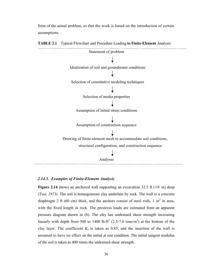
Table 2.1 shows a typical flow chart incorporated in finite-element analyses. The

chart lists the steps involved in the investigation, each step representing an idealized

36

form of the actual problem, so that the work is based on the introduction of certain

assumptions.

TABLE 2.1 Typical Flowchart and Procedure Leading to Finite-Element Analysis

Statement of problem

Idealization of soil and groundwater conditions

Selection of constitutive modeling techniques

Selection of media properties

Assumption of initial stress conditions

Assumption of construction sequence

Drawing of finite-element mesh to accommodate soil conditions,

structural configuration, and construction sequence

Analyses

2.14.3. Examples of Finite-Element Analysis

Figure 2.14 shows an anchored wall supporting an excavation 32.5 ft (10 m) deep

(Tsui, 1973). The soil is homogeneous clay underlain by rock. The wall is a concrete

diaphragm 2 ft (60 cm) thick, and the anchors consist of steel rods, 1 in2 in area,

with the fixed length in rock. The prestress loads are estimated from an apparent

pressure diagram shown in (b). The clay has undrained shear strength increasing

linearly with depth from 500 to 1400 lb/ft2 (2.5-7.0 tons/m2) at the bottom of the

clay layer. The coefficient Ko is taken as 0.85, and the insertion of the wall is

assumed to have no effect on the initial at rest condition. The initial tangent modulus

of the soil is taken as 400 times the undrained shear strength.

37

The assumption of plane strain condition is considered valid for a wall 2 ft thick and

anchor spacing less than 10 ft (3 m).

Fig.2.14

Anchored wall in clay; (a) section through wall; (b) soil data and prestressed diagram. (Tsui, 1973)

A nonlinear elastic model is incorporated in the analysis, and tangent modulus

values are obtained for a stress-strain curve represented by a hyperbola. The

interface between the wall and the soil is treated similarly on both sides using a

bilinear stress-strain deformation relationship with initial shear stiffness 50,000 pcf

reduced by a factor of 1000 if the yield strength of the interface is exceeded.

38

The construction sequence is simulated by an incremented loading process based on

the nine-step modeling shown in Fig.2.15. Anchor lengths vary from 61.5 to 33.9 ft.

Fig.2.15

Construction sequence; Finite element analysis of the anchored wall of Fig.2.14 (Tsui, 1973)

Figures 2.16 and 2.17 show wall and ground movement and earth pressure

distribution, respectively, for the two prestress levels and with zero prestress, together

with anchor loads corresponding to apparent pressure diagrams. Wall movement

responds consistently to prestress level decreasing almost linearly with the amount of

prestressing.

39

Likewise, ground settlement behind the wall decreases as the prestress increases, but

the effect diminishes as the next higher prestress load is introduced. Settlement is thus

reduced more by the first increase than by increases that follow.

Fig.2.16

Wall and ground movements predicted by finite-element analysis; tied-back wall of Fig2.14. (Tsui, 1973)

The predicted earth pressure diagrams shown in Fig.2.17(a) can be compared with the

apparent pressures shown in (b) obtained by distributing the anchor loads over the

appropriate spans. Evidently, the predicted pressures approach the original at-rest

values and exhibit a definite triangular distribution. Interestingly, there are no

pressure bumps at the anchor points.

Fig.2.17

Lateral earth pressure predicted by finite-element analysis, and appearance pressure diagrams, tied-back wall of Fig.2.14. (Tsui, 1973)

40

A second example of anchored wall in day modeled by finite-element analysis is

shown in Fig. 2.18 (Clough and Tsui. 1974). Two cases are investigated, one with

four rows and the other with three rows of anchors. The wall is flexible, with

moderate stiffness equivalent to PZ-72 sheeting. The anchor prestress is likewise

obtained from apparent pressure diagrams.

The predicted lateral pressures are more triangular than the design trapezoidal

diagram, and this distribution is consistent with the actual wall movement. In this

example, unlike the previous case, we can notice that the earth pressures tend to

concentrate slightly at each anchor level. This bulging is caused by the wall

flexibility in response to the application of prestress; hence it must be distinguished

from the linear stress distribution observed with the stiff wall. Its effect is to reduce

the bending moments slightly.

Fig.2.18

Lateral earth pressure behind a flexible wall predicted by finite-element analysis; prestressed tied- back wall. (Clough and Tsui, 1974)

41

By far the greatest use of prestressed anchors is in the support of both temporary

and permanent excavations. A review is given of several case studies to illustrate

the range of problems that have been solved. This is followed by a survey in

summary form of reported anchor uses.

The construction and behaviour of an anchored wall in Genoa is reported by

Barla and Mascardi (1974). A tall building, sited on sloping ground, required an

excavation up to 34m in depth and within 3 m of existing old properties (Fig.2.21).

Fig.2.19

Plan of site showing layout of anchored wall

(Barla and Mascardi, 1974)

The ground conditions were very complex as revealed by 19 boreholes. A section

along the wall is shown in Fig. 2.20. The wall was formed from 358 bored piles at

0.6 to 0.8 m spacing and strengthened with steel H-beams. This wall was tied

back by 658 anchors, Tirsol type IRP, inclined at 20° to the horizontal with

working loads between 569 and 853 kN. Fourteen rows of steel wale beams linked

the heads of the prestressed anchors to the piled wall, Fig.2.21.

It will be noted that the bored piles were intialty taken to an intermediate level to

ensure that they did not deviate from the vertical, otherwise difficulties would

arise with wale beam attachment. The excavation proceeded step by step as the

42

anchors were installed and the order of the main stages of the excavation is given

in Fig.2.22. The initial design was based on a triangular earth pressure

distribution assumption. The excavation process was simulated by a finite element

study. This showed that the most critical zone was an area of stiff silty clay. The

wall was carefully monitored during and after construction and comparisons

made between field measurement and finite element prediction. Very good

agreement was found, thus confirming that a good estimate had been made of the

ground parameters and of the in-situ stress state in the ground.

Fig.2.20

Vertical section along anchored retaining wall showing various stages of excavation

(After Barla and Mascardi, 1974)

43

Fig.2.21

Vertical cross-section through the anchored wall (After Barla and Mascardi, 1974)

Fig.2.22

Anchored diaphragm wall for CPF building, Singapore (After Littlejohn and MacFarlane, 1974)

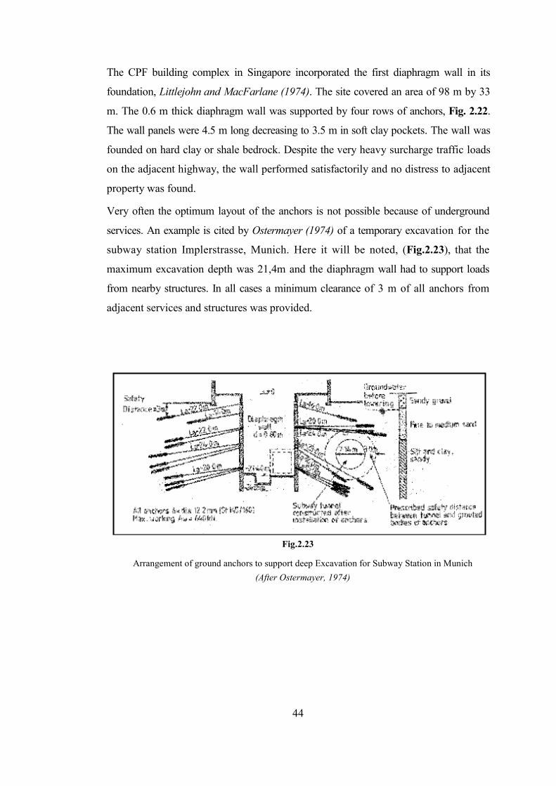
44

The CPF building complex in Singapore incorporated the first diaphragm wall in its

foundation, Littlejohn and MacFarlane (1974). The site covered an area of 98 m by 33

m. The 0.6 m thick diaphragm wall was supported by four rows of anchors, Fig. 2.22.

The wall panels were 4.5 m long decreasing to 3.5 m in soft clay pockets. The wall was

founded on hard clay or shale bedrock. Despite the very heavy surcharge traffic loads

on the adjacent highway, the wall performed satisfactorily and no distress to adjacent

property was found.

Very often the optimum layout of the anchors is not possible because of underground

services. An example is cited by Ostermayer (1974) of a temporary excavation for the

subway station Implerstrasse, Munich. Here it will be noted, (Fig.2.23), that the

maximum excavation depth was 21,4m and the diaphragm wall had to support loads

from nearby structures. In all cases a minimum clearance of 3 m of all anchors from

adjacent services and structures was provided.

Fig.2.23

Arrangement of ground anchors to support deep Excavation for Subway Station in Munich

(After Ostermayer, 1974)

45

This finite element analysis is an example from Switzerland which is “Cut and Cover Tunnel

with Sheet Pile Walls used as Anchor Walls”. The plain between Solothurn and Biel,

specially the so called Grenchner Witi, is one of the most important swamp areas of

Switzerland and is therefore protected by law. For this reason the new motorway

between Solothurn and Biel crosses the central part of this protected area in a tunnel.

The motorway section was built as a cut and cover tunnel. Because the installation of

ground anchors in the saturated, loose to medium dense fine sands was a mayor risk

with regard to the time schedule, the contractor made an alternative proposal with two

sheet pile walls used as anchor walls. These anchor walls had a length of 12 m and

were driven at 14 m distance from the main sheet pile walls. From the main sheet pile

wall anchor rods were drilled to the anchor wall. The distance between the single

anchor rods was 4 m.

As a first step the 12 m long anchor walls were driven into the soil in two rows at a

distance of 58 m. A first excavation step with slopes on each side was cut down to a

depth of -4,10 m within the anchor walls (see Fig. 2.24). From this level the 18 m

long main sheet pile walls were driven at a distance of approximately 50 m from each

other respectively at 14 m from the anchor walls (see Fig.2.24). The next

excavation phase within the main sheet pile walls reached the level of -7,00 m,

Now the 14 m long achor rods were drilled from the main sheet pile wall to the

anchor wall at a distance of 4 m. After their prestressing to 1000 kN the

excavation could proceed to the final depth of -10.70 m. The lowering of the

groundwater table was performed by deep wells located in the centre of the

excavation and along the inner sides of the main sheet pile walls, The depth level of

the wells was 2 m less than the tip of the main sheet pile walls. Thanks to the safe

and quick anchoring system two tunnel sections of 12.5 m length could be

constructed each week.

46

Fig.2.24

Cross Section

For this case analysis insitu measurements were also performed at several typical

cross sections which includes, inclinometer at main sheet pile wall, inclinometer at

anchor wall, tensile force in anchor rod, groundwater table.

The maximum measured deformations are about 77 %.of the calculated ones. The

tensile force in the anchor rod was measured to be 820 kN after the final

excavation. Before the last excavation step the prestressing in the anchor rod was 1000

kN. Therefore a drop of 180 kN during excavation was measured.

In the original safety documents for the main sheet pile wall combined with

prestressed ground anchors the allowable horizontal deformations were set to

50 mm. For alternative design, the allowable deformations of the main sheet pile wall

were kept at 50 mm, the allowable deformations of the anchor wall were limited to

170 mm in accordance with the predicted PLAXIS deformations, Due to the absence

of any buildings and other facilities such large deformations could be tolerated.

The calculated deformations of the main sheet pile wall and the anchor wall

coincide reasonably well with the measured maximum deformations. The smaller

measured values can be explained with a deeper actual groundwater table (due to

dewatehng), better soil properties and a smaller thickness of the weak surface layers,

Furthermore the magnitude of prestressing force in the calculation model was

47

assumed to be 1200 kN (300 kN/m) instead of 1000 kN in reality, leading as well to

smaller deformations mainly at the anchor wall.

This study, taken from a case study applied in the Longwood Medical Area, Boston,

USA, summarizes the performance of the lateral earth support system based on field

monitoring data measured during excavation of the basement. Back analyses are then

used to evaluate and interpret the wall and ground movements.

Fig.2.25

Measured and predicted behavior of Section A-A walls early stages of excavation

Fig.2.25 compare the measured wall deflections and surface settlements at the south

and north walls at selected stages of excavation. The results show a small (5 mm)

inward cantilever deflection of the north wall. However, subsequent excavation and

prestressing of anchors causes a reversal in wall deflections such that there is a small

net outward movement (up to 6 mm) at the end of the excavation. The toe of the wall

rotates but shows no net displacement.

48

Fig.2.26

Measured and predicted behavior of Section B-B walls early stages of excavation

Figure 2.26 shows analogous results for the East and West walls (section B-B). Both

walls show excellent toe fixity and both are prestressed such that there are maximum

net outward movements up to 15 mm (and quite similar deflection mode shapes).

Settlements behind the East wall were measured at a series of reference points inside

the utility tunnel (Figs. 2.26b). These data show very small settlements through the

early phases of excavation (less than 3mm at stage P3). However, there are large

increments of settlements associated with installation of tieback anchors at level P4

and further increases during the remainder of the excavation. Maximum settlements

of the utility tunnel beneath Binney Street exceeded 70 mm by the end of excavation.

There was a similar pattern of measured surface settlements for the Redstone

Building, with maximum settlements up to 64 mm.

A series of finite element simulations have been carried out to obtain better insight into

the performance of the excavation support system for the Dana Farber research tower.

The calculations have been carried out using the Plaxis finite element code (Brinkgreve,

2002) and comprise a series of four 2-D, plane strain models representing each of the

four sides of the excavation. Given the almost complete lack of site specific data on soil

deformation and shear strength properties, these parameters have been estimated

based on prior experience, published correlations and case studies in the Boston area

(e.g., Duncan et al., 1980; Johnson, 1989; Ladd et al., 1999; Altabba & Whittle, 2001;

Hashash & Whittle, 1996). The soil parameters have subsequently been refined in back-

49

analyses for the North wall section. Each of the soil layers has been simulated using the

Hardening Soil (HS) model (Schanz et al., 1999). This model represents an updated

version of the well known Duncan-Chang model (Duncan et al., 1980), formulated using

elasto-plasticity. The non-linear shear-stress strain behavior in loading is represented

by a hyperbolic function (with average secant modulus, E50, Fig. 2.27); while a much

stiffer linear response in unloading is described by the parameter, Eur. The shear

strength is characterized by conventional Mohr-Coulomb parameters (c’, φ'). The HS

model enables a realistic description of the stiffness of the retained soil relative to the

excavated material with minimal additional parameters.

Fig.2.27

Shear stress-strain behavior of Hardening Soil (HS) model (Schanz et al., 1999)

50

CHAPTER III

FIELD STUDIES

The subway construction of Ulus – Keçiören has a length of 9685 m which is

constructed under the extension of Ankara Metropolitan Municipality and the

transportation plan of General Directorate of EGO. The route of Ulus – Keçiören

metro construction starts from the Gençlik Parkı station and ends at the Gazino

junction.

Fig. 3.1

The route of Ulus-Keçiören Metro Project

51

The route of Ulus – Keçiören metro is investigated geologically, and the drilling bore

hole’s studies and the laboratory tests are performed. The results were reported by

Yüksel Proje A.Ş. with respect to site investigations, drilling logs, in-situ and

laboratory experiments.

3.1. Geological Studies

The geological map of the route of the subway construction is obtained from the site

investigations and bore hole logs. Totally 43 bore hole were carried out along this

route which covers a depth of 1169,37 m to determine the geological and

geotechnical properties of the rock and soil.

The elevations, coordinates and depths of the bore hole logs and estimated ground

water table levels are given in Table 3.1 around the Gazino district.

Table 3.1.

Bore Hole Logs of Gazino district

DEPTH GROUND WATER LEVEL

BORE HOLE LOG

KM

(m) (m)

UK-29 7+013 27 4.20

UK-30 7+076 27 3.95

UK-31 7+547 34 8.40

UK-32 7+986 42 4.85

UK-33 8+445 38 11.40

UK-34 8+528 37 4.80

UK-35 8+899 39 0.95

UK-36 9+374 34 4.10

UK-37 9+470 34 5.20

UK-38 9+559 42 7.20

UK-39 0+762 18.45 5.15

YT-1 7+637 17 5.85

YT-2 7+676 22 ARTESIAN

YT-3 7+789 36 ARTESIAN

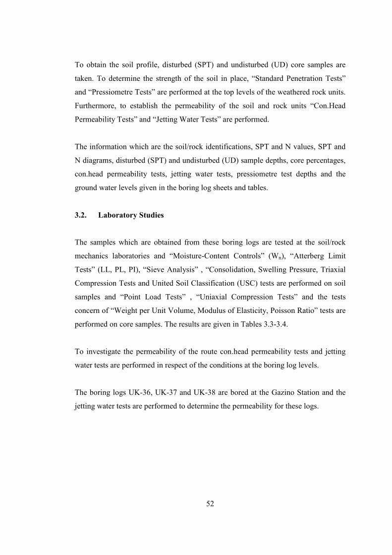
52

To obtain the soil profile, disturbed (SPT) and undisturbed (UD) core samples are

taken. To determine the strength of the soil in place, “Standard Penetration Tests”

and “Pressiometre Tests” are performed at the top levels of the weathered rock units.

Furthermore, to establish the permeability of the soil and rock units “Con.Head

Permeability Tests” and “Jetting Water Tests” are performed.

The information which are the soil/rock identifications, SPT and N values, SPT and

N diagrams, disturbed (SPT) and undisturbed (UD) sample depths, core percentages,

con.head permeability tests, jetting water tests, pressiometre test depths and the

ground water levels given in the boring log sheets and tables.

3.2. Laboratory Studies

The samples which are obtained from these boring logs are tested at the soil/rock

mechanics laboratories and “Moisture-Content Controls” (Wn), “Atterberg Limit

Tests” (LL, PL, PI), “Sieve Analysis” , “Consolidation, Swelling Pressure, Triaxial

Compression Tests and United Soil Classification (USC) tests are performed on soil

samples and “Point Load Tests” , “Uniaxial Compression Tests” and the tests

concern of “Weight per Unit Volume, Modulus of Elasticity, Poisson Ratio” tests are

performed on core samples. The results are given in Tables 3.3-3.4.

To investigate the permeability of the route con.head permeability tests and jetting

water tests are performed in respect of the conditions at the boring log levels.

The boring logs UK-36, UK-37 and UK-38 are bored at the Gazino Station and the

jetting water tests are performed to determine the permeability for these logs.

53

Table 3.2 Jetting Water Test Results for Gazino Station

Table 3.3 Soil Mechanics Laboratory Test Results

* Wn is the water percent

Table 3.4 Weight per Unit Volume (γ) and Uniaxial Compressive Strength (UCS) Test Results

SAMPLE

ATTERBERG LIMITS

SIEVE ANALYSIS

BORE HOLE LOG

SAMPLE NO

DEPTH

(m)

Wn*

(%) LL (%)

PL (%)

PI +4 (%)

-200 (%)

SOIL CL.

(USCS)

UK-36 SPT-2 3.00-3.45 20 35 17 18 3 40 SC SPT-4 7.50-7.95 20 39 23 16 4 50 CL SPT-7 12.00-

12.45 33 63 33 30 - 62 MH

UK-37 SPT-2 3.00-3.45 18 44 23 21 4 36 SC SPT-4 6.00-6.27 17 51 32 19 37 26 SM/GM

UK-38 SPT-2 3.00-3.45 22 57 33 24 7 58 MH SPT-3 4.50-4.95 11 - NP - 63 9 GW/GM

BORING LOG

DEPTH of WELL (m)

LENGTH of LAYER(m)

DEG. Of LEGEON

EXPLANATIONS

UK-36 34.00 1.70 Lu>25 Highly Permeable UK-36 34.00 1.70 1.34 Low Permeable UK-36 34.00 1.70 2.56 Low Permeable UK-37 34.00 1.70 Lu>25 Highly Permeable UK-37 34.00 1.70 Lu>25 Highly Permeable UK-37 34.00 1.70 3.81 Low Permeable UK-37 34.00 1.70 2.67 Low Permeable UK-38 42.00 1.70 - Cannot measured UK-38 42.00 1.70 6.09 Permeable

SAMPLE NO DEPTH

(m) γγγγ

(kN/m3) UCS (MPa)

UK-36 K5 15.00-16.50 21.64 14 UK-36 K7 18.00-19.50 23.38 22 UK-36 K16 31.50-33.00 23.38 23 UK-37 K5 12.00-13.50 25.03 78 UK-37 K12 22.50-24.00 24.55 80 UK-37 K15 22.00-28.50 23.06 41 UK-38 K16 25.50-27.00 24.59 53

54

3.3. Geotechnical Evaluation

The ground formation of the Gazino Station is formed by units of igneous series. The

average depth of excavation is about 29 m. The excavation takes progress in the

formation of agglomerate/agglomerated tuff which is highly weathered at top levels

and has a color of brown-claret red, andesite which is stiff-moderate stiff and soft in

some parts (top levels), strong-moderate strong and weak in some parts, slightly

weathered-fresh and moderately weathered-highly weathered at top levels and has a

color of brown-gray and andesite tuff which is moderately-highly weathered and

completely weathered in some parts and has a color of gray-greenish and gray. These

formations are observed lateral transitive with each others.

3.3.1. General Geology

The main geological formation of Ankara is given in the Fig.3.2 below.

Fig. 3.2

Main geological map of Ankara

55

Qal : Alluvium (Qal) Clay, Sand, Gravel

Te : Etimesgut Formation (Te) Ankara Clay (Ak)

Silty Clay, Sandy Clay, Gravelly and Sandy Clay

Tb Bozbağ Basalt

Basalt

Tf Igneous Series (Vs) Tekke Volcanite

Andesite, Trakiandesite, Tuff, Agglomerate

Tma Mamak Formation

Agglomerate, Tuff, Andesite

3.3.2. Local Geology

The main geological formations which observed at the route of Ulus – Keçiören

subway are Hançili Formation, Igneous Series (Vs), Ankara Clay (Ak) and

Alluvium. These formations are covered with dumped fill at the top levels.

Hançili Formation

This formation is formed by clay limestone, marn, siltstone, sandstone, conglomerate

and a line arrangement of tuffite and comprises gypsum and bituminous shale in

some parts. Besides, andesite fibers are observed. Clay limestone and marns are

white-yellow white in color, thin layered and followed by siltstone-sandstone.

Siltstones are gray in color, thin layered and laminated. Conglomerate and

sandstones are yellowish and layered indeterminate.

56

Igneous Series (Vs)

This formation is formed by andesite, basalt, tuff and agglomerate in general.

Agglomerates in the formation are formed by andesite and basalt gravels which are

white, gray and red in color and attached by tuff. Clear stratification is observed in

some parts. The thin layered and different colored tuffs and andesite can be observed

in agglomerate form. Andesite is red, pink, grey and black colored. Basalts are black-

dark brown colored and weathered.

Ankara Clay (Ak)

Ankara Clay is formed by the sedimentation of fine grained stream sediments at the

flood plains. The main formation is fine-grained sediments but in some parts sand-

gravel levels can also be observed.

Ankara Clay is observed in red, brown, beige colors, and fissured, sand-gravel levels

can be seen in some parts, and shows the properties of low-high plasticity, very hard-

stiff, overconsolidated silty clay and sandy clay.

Alluvium (Qal)

The alluvial sediments are in general greenish and gray-brown in color and formed

by a mix of moderate-high plasticity, hard-very hard sandy and silty clay and clayey

sand, clayey-sandy gravel levels.

Dumped Fill (Yd)

The dumped fill which covers the route is a part of the soil/rock materials that are

obtained from the excavation and digging of the route.

The underground water levels which are measured from the boring logs given in

Table 3.2 and to determine the permeability of the soil/rock units the con.head

permeability tests and jetting water tests are performed and results are given in

Table 3.3.

57

The construction of Gazino Station is formed by various phases and as these phases

commence the site studies are observed and the pile deformation measurements are

obtained from these site studies.

Fig.3.3 General Geology of Gazino Station

Dumped Fill

Sandy Clay

Agglomearte, Tuff

Agglomearte, Tuff

Tuff

Andesite

Andesite, Tuff

Dasite, Tuff

Piles

58

CHAPTER IV

MODELLING OF GAZİNO STATION ANCHORED PILE WALL

The study involves the dry construction of the Gazino Station as the ground water

level always kept under excavation level. The excavation is supported by concrete

sheet pile walls. The walls are tied back by pre-stressed ground anchors. Plaxis

allows for a detailed modelling of this type of problem. Actually during the

excavation and construction work no problems occured and the study has been made

to investigate the sheet pile walls behaviors under the determined soil properties and

site conditions.

4.1. Layout Plan of Gazino Station

The average excavation is about 20 m wide and 29 m deep. The plan view of the site

is shown in Fig. 4.1. The used average length of concrete sheet piles to retain the

surrounding soil is 10 m and 0,80 m in thickness. Two or five rows of ground

anchors are used at each wall to support the walls.

The upper anchor has a total free length of 14 m and a total fixed length of 8 m and

an inclination of 15o. The free length of lower anchor is 6 m and a fixed length of

8m. The analysed section taken for the modeling purpose of Gazion station is given

in Fig. 4.2.

59

Fig

.4.1 Plan view

of Gazino Station

A A’

60

Fig. 4.2

A-A’ section view of the Gazino Station

4.2. Prediction of Soil and Rock Properties of the Model

The relevant part of the soil consists of three distinct (at some parts two) layers.

From the ground surface to a depth of approximately 3 m there is a fill of stiff sandy

and silty soil. Underneath the fill, down to a minimum depth of app. 10 m, there is

more or less homogeneous layer consisting of sandy clay. Below the sandy clay layer

there is an andesite layer which is moderately weathered and highly weathered in

some parts and moderately strong and moderately weak and weak in some parts and

extends to large depth. All of the layers are suitable for the installation of the ground

anchors. In the initial situation there is a horizontal phreatic level at average depth of

6 m below the ground surface.

entrance

STRUCTURE

61

Disturbed and undisturbed soil samples were taken from the various depths of

boreholes. Standard laboratory tests were performed on these samples to obtain the

grain size distribution, water content, plastic limit and liquid limit of the soil layers. The

soil samples are classified according to the results of these tests by using the Unified

Soil Classification system. Besides the laboratory tests mentioned above, SPT tests

are performed at regular intervals at the boreholes to determine the stiffness or

consistency of the soils. A summary of the borehole data is shown in Fig. 4.3.

After investigating the borehole data the soil profile is idealized as follows:

0-3.0m - Dumped Fill : This layer can be identified as sandy clay and gravel soil.

Excluding a few high values, possibly due to gravel or large objects, the average

value of SPT blow count number is 9. Characteristic values for Plastic Limit (PL),

Liquid Limit (LL) and Plasticity Index (PI) for this layer are given below :

PL = 2 3%

LL = 44%

PI =21%

62

Fig.4.3 Drilling Log Sheet SPT and Pressuremeter Test Results

63

Table 4.1 Consistency of clays and approximate correlation to the standard penetration number, N (Das, 1984)

SPT, N, number of 9 gives an idea about the consistency of the soil and the soil may

be classified as medium stiff clay (See Table 4.1). As a representative value for

medium stiff clay, the unit weight may be taken as γ = 17,5 kN/m3 (See Table 4.2).

Table 4.2

Typical ground parameters (Carter&Bentley, 1991)

64

To predict the effective stress parameters, c and φ, the correlations with the plasticity

index, PI, of cohesive soils were used. Two of these correlations are summarized

below:

PI = 21 ------------- ► φ = 22° (See Figure 4.4)

PI = 21------------- ► φ = 31° (See Figure 4.5)

Therefore , as a representative value, φ is taken as 27°.

Fig. 4.4 Relationships between angle of shearing resistance and plasticity index

(Carter&Bentley, 1991)

For the determination of the drained Young's modulus of elasticity, Ed, a well known

correlation is, Ed = 1 / mv, where mv is the coefficient of the volume of compressibility.

Stroud (1974) gives a correlation between mv and N as :

mv = 1 / f2. N

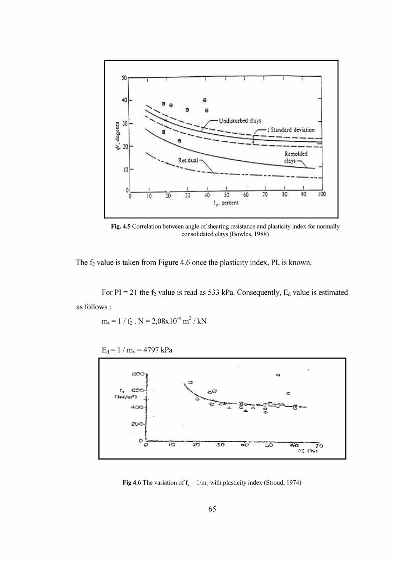
65

Fig. 4.5 Correlation between angle of shearing resistance and plasticity index for normally consolidated clays (Bowles, 1988)

The f2 value is taken from Figure 4.6 once the plasticity index, PI, is known.

For PI = 21 the f2 value is read as 533 kPa. Consequently, Ed value is estimated

as follows :

mv = 1 / f2 . N = 2,08x10-4 m2 / kN

Ed = 1 / mv = 4797 kPa

Fig 4.6 The variation of f2 = 1/mv with plasticity index (Stroud, 1974)

66

Another way to estimate the value of Ed is to use the results of the Cone Penetration

Test (CPT) results. Although, there are no CPT results for the problem at hand, one may

use the correlations between the SPT and CPT values. Lunne et.al. (1997) recommend

the following relation for the estimation of CPT, qc, values from SPT, N, values.

Clayey silt to silty clay ----------► qc / N = 2 (See Table 4.3)

qc = 2 x 9 = 18 kg / cm2 = 1800 kPa

Once qc value is determined, it is possible to use the relations that relate qc to Ed as

follows :

Table 4.3

Soil classification and CPT-SPT correlations (Lunne, Robertson&Powell, 1997)

67

Ed = αm. qc

qc=1,8 MPa αm = 2 (See Table 4.4)

Ed = 2x1800 = 3600 kPa

Therefore, as a representative value, Ed is taken as 4000 kPa.

γ = 17,5 kN/m3

Effective stress (drained) parameters :

c = 0 (cohesionless dumped fill) φ = 27°

Ed = 4000 kPa, νd = 0,353

Table 4.4 Estimation of constrained modulus, M, for clays (Lunne,

Robertson%Powell, 1997)

68

3,0 - 8,0 m - Sandy Clay : This layer can be identified as sandy clay (CL). Excluding a

few high values, possibly due to coarse gravel or large objects, the average value of

SPT blow count number, Nav, is 13. Characteristic values for Plastic Limit (PL),

Liquid Limit (LL) and Plasticity Index (PI) for this layer are given below :

PL =32% PI = 19

LL = 51 %

The soil may be classified as hard clay due to the average SPT blow count number, N,

of 36. (See Table 4.1) . As a representative value for hard clay, the unit weight may be

taken as γ = 20,0 kN/m3 (See Table 4.2).

Using the correlations between PI and φ, the effective soil friction angle φ is

estimated as follows:

PI = 19 --------------► φ = 24° (See Figure 4.4)

PI = 19---------------► φ = 32° (See Figure 4.5)

Therefore, as a representative value, φ is taken as 28°.

The drained Young's modulus of elasticity, Ed, is estimated using the

procedure recommended by Stroud (1974) as explained before.

Ed = 1 / mv, where mv is the coefficient of the volume of compressibility.

mv = 1 / f2. N

The f2 value is taken from Figure 4.7 once the plasticity index, PI, is known. For PI =

19 the f2 value is read as 566 kPa. Consequently, Ed value is estimated as follows:

69

mv = 1 / f2 . N = x10-4 m2 / kN

Ed = 1 / mv = 20376 kPa

Another estimation for Ed is obtained by using the CPT correlations. Firstly, the CPT

data is estimated from SPT results as follows:

Clayey silt to silty clay --------------------► qc / N = 2 (See Table 4.3)

qc = 2 x 36 = 72 kg / cm2 = 7200 kPa

Once qc value is determined, it is possible to use the relations that relate qc to Ed as

follows: Ed = αm . qc

qc = 7,2 MPa , CL αm = 3,5 (See Table 4.4)

Ed =3,5x7200 = 25200 kPa

Therefore, as a representative value, Ed is estimated as 20000 kPa.

γ = 20,0 kN/m3

Effective stress (drained) parameters :

c = 0 , φ = 28o

Ed = 20000 kPa

νd = 0,346

8,0 - 29,0m – Andesite Layer: Excluding thin layers of clay encountered at

boring locations, this layer can be identified as andesite.

The soil has an average unit weight value of γ = 24 kN/m3 due to the tests and

boring log values.

For the estimation of effective internal friction angle, φ some

recommendations relating relative density with φ are available.

70

Table 4.5 Empirical values for φ, Dr, and unit weight of granular soils based on the

SPT at about 6 m depth and normally consolidated (Bowles, 1988)

Table 4.6 Relation between N-values, relative density, and angle of friction in sands

(Das, 1984).

71

Fig.4.7

Plot of standard penetration resistance vs. angle of friction for granular soils (Das, 1983)

As no further SPT results are obtained for this layer, as a representative value, φ is taken as 40°.

For estimation of Ed values it is possible to use the boring log data sheet and an average

value can be obtained.

Due to the boring log sheet an average Ed value can be taken as 66000 kN/m2

Therefore, as a representative value, Ed is estimated as 200000 kPa.

Andesite layer is moderately weathered and moderately weak at top layers but

moderately strong and slightly weathered and stiff at below parts. The Young’s

Modulus of this layer is increased due to the depth of the soil.

The selected parameters as a result of the discussions presented above are

summarized below :

72

γ = 24,0 kN/m3

Effective stress (drained) parameters :

c = 100 kPa

φ = 40°

Ed = 100000 kPa

νd = 0,263

c (cohesion) value is taken as “0”. In Plaxis c value is entered as 0,2 kPa in case of

avoid complications.

Soil cohesion value is taken as 10 kPa for Sandy Clay according to SPT N value and

the estimation which is given by Stroud (1974) as below:

cu = f1 . N

f1 value is obtained from correlation of SPT resistance diagram (Fig.4.8),

(NAVFAC DM-7.1).

c value can be selected as 100 kPa for andesite layer.

Fig. 4.8 Correlation of standard penetration resistance (NAVFAC DM-7.1)

73

4.3. Geometry of Model

The problem can be modeled with a geometry model of 35 m width and 20 m depth. A

ground anchor can be modeled by a combination of a node-to-node anchor and a

geotextile. The geotextile simulates the grout body whereas the node-to-node anchor

simulates the anchor rod. In reality there is a complex three dimensional state of stress

around the grout body. Although the precise stress state and interaction with the soil

cannot be modeled with this 2D model, it is possible in this way to estimate the stress

distribution, the deformations and the stability of the structure on a global level,

assuming that the grout body does not slip relative to the soil. With this model it is

certainly not possible to evaluate the pull-out force of the ground anchor.

The pile wall is modeled as a beam. The interfaces around the beam are used to model

soil-structure interaction effects. They are extended under the wall for 1,0 m. Interfaces

should not be used around the geotextiles that represent the grout body.

The excavation is constructed in several excavation stages. The separation between the

stages is modeled by geometry lines.

The water table is below the excavation level but initially there is a water level of -6m and

water pressures generated initially. As the excavation commences water drained and no

groundwater is observed during excavation stages. The schematic view of the anlaysed

model of the studied section of the Gazino station is given in Fig. 4.9.

74

Fig.4.9

Modeled section

4.4. Material properties of the Model

The soil consists of three (in some sections two) distinct layers. Three data sets for soil &

interfaces with the parameters given in Table 4.7. The beam elements used to model the

walls are, on their own, fully permeable. Therefore, the interfaces around the wall

must be used to block the flow through the wall for groundwater calculations and

consolidation analyses. This can be achieved by setting the permeability parameter of the

interface to Impermeable. In that case a very low (but non zero) value of the interface

permeability is used. For the interfaces in the loam layer below the wall (the extended

part of the interfaces) the strength reduction factor is set to Rigid (no reduction) and the

permeability parameter is set to Neutral.

The properties of the concrete pile are entered in a material set of the beam type. The

concrete has a Young’s modulus of 30 GPa and a thickness of 0,8 m (for pile). The

properties are listed in tables

CL

Dumped Fill c=0 kPa φ=270

E=4000 kPa

Andesite c=100 kPa φ=400 E=200000 kPa

8,0 m

8,0 m

10,0 – 15,0 m

9,0 m

8,0 m Sandy Clay c=10 kPa φ=280 E=20000 kPa

Excavation

Structure

75

Table 4.7 Soil and interface properties

Parameter Name Fill Sandy Clay Andesite Unit

Material model Model MC MC MC

Type of material behaviour Type drained drained drained -

Dry soil weight γdry 17,5 20 24 kN/m3

Wet soil weight γwet 19 23 27 kN/m3 Horizontal permeability Kx 0 0 0 m/day

Vertical permeability Ky 0 0 0 m/day

Young's modulus Etef 4000 20000 200000 kN/m2

Poisson's ratio ν 0,353 0,346 0,263 - Cohesion Cref 0,2 10 100 kN/m2

Friction angle φ 27 28 40 0

Dilatancy angle ψ 0 0 10 o

Interface reduction factor Rinter Rigid Rigid Rigid -

Interf Permeability Perm. -

Table 4.8 Properties of the pile (beam)

Parameter Name Value Unit

Type of behaviour Material type Elastic _

Normal stiffness EA 2,4-107 kN/m

Flexural rigidity El 1,28-106 kNm/m

Equivalent thickness D 0,80 m Weight W 19,2 kN/m/m Poisson's ratio ν 0,15 -

Table 4.9 Properties of the pile cap (beam)

Parameter Name Value Unit

Type of behaviour Material type Elastic _

Normal stiffness EA 1,5-107 kN/m Flexural rigidity El 3,125-105 kNm/m

Equivalent thickness D 0.50 m

Weight W 12 kN/m/m

Poisson's ratio ν 0,15 -

76

Beams are composed of beam elements with three degrees of freedom per node: Two

translational degrees of freedom (ux and uy) and one rotational degree of freedom

(rotation in the x-y plane: θz). When 6-node soil elements are employed then each beam

element is defined by 3 nodes whereas 5-node beam elements are used together with the

15-node soil elements. The beam elements are based on Mindlin’s beam theory. This

theory allows for beam deflections due to shearing as well as bending. In addition, the

element can change length when an axial force is applied. Beam elements can become

plastic if a prescribed maximum bending moment or maximum axial force is reached.

Stress points

Nodes

Fig. 4.10

Position of nodes and stress points in a 3-node beam element

The material properties of beams are contained in material data sets. The most important

parameters are the flexural rigidity (bending stiffness) EI and the axial stiffness EA.

From these two parameters an equivalent beam thickness is calculated from the equation

below.

EA

EId 12= d: beam thickness (4.1)

Bending moments and axial forces are evaluated from the stresses at the stress points. A

3-node beam element contains two pairs of stress points whereas a 5-node beam

element contains four pairs of stress points. Within each pair, stress points are located at

a specific distance above and below the beam centre-line:

3/d (4.2)

For elastic behavior an axial stiffness, EA and a flexural rigidity, EI, should be specified

as material properties. The values of EA and EI relate to a stiffness per unit width in the

77

out-of-plane direction. Hence, the axial stiffness, EA is given in force per unit width and

the flexural rigidity, EI is given in force length squared per unit width.

Beam Element (Pile)

E = 3,0.107 kN/m2 (concrete)

L = 1m A = 0,8x1 = 0.8 m2

EA = 2,4.107 kN EI is calculated from

d=0.8m EA

EId 12=

Beam Element (Pile Cap)

d =0.5 m E = 3,0.107 kN/m2 (concrete)

L = 1 m A = 0,5x1 = 0,5 m2

EA = 1,5.107kN

For the properties of the ground anchors, two material data sets are needed: One of the

Anchor type and one of the Geotextile type. The Anchor data set contains the

properties of the anchor rod and the Geotextile data set contains the properties of the

grout body. The data are listed in table 4.10 and informations on anchorages are given

below.

Applying of anchorages: 3 rows

Anchorage spaces: 1,6 m

Anchorage slope: 15o

Anchorage Capacity: 30 tons

78

Table 4.10 Properties of the anchor rod (node-to-node anchors)

Parameter Name Value Unit

Type of behaviour

Normal stiffness

Spacing out of plane

Maximum force

Material type

EA

Ls

Elastic

128000

1,6

kN

kN

m

A material data set for anchors may contain the properties of Node-to-node anchors

as well as Fixed-end anchors. In both cases the anchor is just a spring element. The

major anchor property is the axial stiffness, EA, entered per anchor and not per unit

width in the out-of-plane direction. In order to calculate an equivalent stiffness per

unit width, the out-of-plane spacing, Ls, must be entered. If the material type is

selected as elastoplastic, a maximum anchor force, Fmax, can be entered (also per

anchor). In the same way as the stiffness, the maximum anchor force is divided by

the out-of-plane spacing in order to obtain the proper maximum force in a plane

strain analysis. If the material type is set to elastic (the default setting), the maximum

force is set to 1•1015 units.

Anchors can be pre-stressed in a Staged construction calculation. In such a

calculation the pre-stress force for a certain calculation phase can directly be given in

the anchor property window. The pre-stress force is not considered to be a material

property and is therefore not included in an anchor data set.

Table 4.11. Property of the grout body (geotextile)

Parameter Name Value Unit

Normal stiffness EA 3,0-106 kN/m

Geotextiles are flexible elastic elements that represent a sheet of fabric in the out-

of-plane direction. The only property in a geotextile data set is the elastic axial

stiffness, EA, entered in units of force per unit width. The axial stiffness, EA, can

be determined by multiplying the Young's modulus of the geotextile material by

the thickness of the fabric. Geotextiles cannot sustain compressive forces.

79

4.5. Mesh generation of the Model

For the generation of the mesh it is set the very coarseness parameter.

Fig.4.11

Plaxis Model

In the initial conditions, a water weight of 10 kN/m3 is entered. The water level is at 6

m below surface and initially a phreatic line is generated. As the water level is below

the excavation levels water is drained during excavation.

Initially, all structural components are deactivated. The initial stress field is generated by

means of the K0-procedure using the values calculated by the formula in all clusters.

K0 values are calculated by Plaxis using the Jaky’s Formula which is

φsin1Ko −= (4.3)

80

After the geometry of the problem is defined and the beam, anchorage and interface

elements are positioned, the boundary conditions are introduced. The boundary

conditions imply rollers at the vertical sides and full fixity at the base of the mesh.

The groundwater conditions are specified by a phreatic line which is lowered as the

excavation proceeds. By this way it is possible to get more realistic results at the

intermediate construction stages.

For c > 0, the Mohr-Coulomb model allows for tension. In fact allowable tension

stresses increase with cohesion. This behaviour can be included in a PLAXIS

analysis by specifying a so-called tension cut-off. In this case, Mohr circles with

negative principal stresses are not allowed. The tension cut-off introduces three

additional yield functions, defined as:

014 ≥−= tf σσ (4.4)

025 ≥−= tf σσ (4.5)

036 ≥−= tf σσ (4.6)

On using the tension cut-off, the allowable tensile stress at is taken equal to zero. For

these three yield functions an associated flow rule is adopted. For stress states within

the yield surface, the behaviour is elastic and obeys Hooke’s law for isotropic linear

elasticity. Hence, besides the plasticity parameter, input is required of the elastic

shear modulus G and Poisson’s ratio ν.

Conclusively, the Mohr-Coulomb model requires five parameters in total:

Shear modulus G = E / 2 (1+v) ( E = Young’s Modulus)

Poisson’s ratio ν

Friction angle φ

Cohesion c

Dilatancy angle ψ

81

Most soils show an increase of stiffness with mean stress level. The influence of the

stress level on the material stiffness can be simply formulated as a power law:

G = Gref (p*/pref)m (4.7)

where, Gref is a reference shear modulus for a particular reference pressure pref

(usually 100 kPa). The power m in equation 4.7 determines the influence of the

stress level on the stiffness, typical values are around 0.5.

The behaviour explained above is modeling by the Advanced Mohr Coulomb model in

PLAXIS. Standard Mohr Coulomb model is used for the cohesive soil layers while

the Advanced Mohr Coulomb model is thought to be more appropriate to use for

modeling the granular soil layers for the problem at hand.

In order to simulate the conditions at site before the excavation, the initial stresses are

generated at the soil media by using a coefficient of lateral earth pressure of Ko

and by turning on the weight of the soil elements while turning off the weight of the

beam elements. After the initial stresses are generated, the excavation is modeled

by switching off the necessary soil elements for each construction stage and the

plastic calculations are carried out.

4.6. K0 Procedure in Plaxis

The initial stresses in a soil body are influenced by the weight of the material and

the history of its formation. This stress state is usually utilized by an initial vertical

stress σv,0 which is related by the coefficient of lateral earth pressure K0 (σh,0 =

K0.σv,0). In PLAXIS initial stresses may be generated by specifying K0 or by using

Gravity loading. ΣMweight:

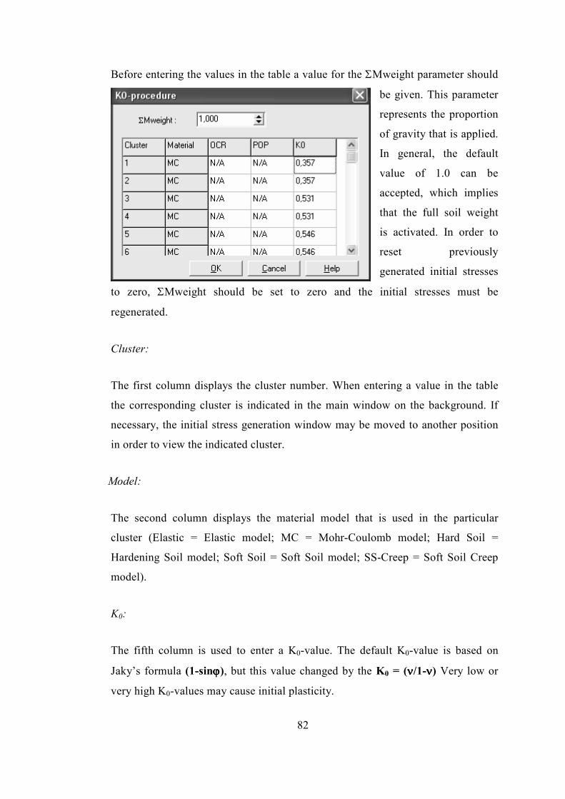
82

Before entering the values in the table a value for the ΣMweight parameter should

be given. This parameter

represents the proportion

of gravity that is applied.

In general, the default

value of 1.0 can be

accepted, which implies

that the full soil weight

is activated. In order to

reset previously

generated initial stresses

to zero, ΣMweight should be set to zero and the initial stresses must be

regenerated.

Cluster:

The first column displays the cluster number. When entering a value in the table

the corresponding cluster is indicated in the main window on the background. If

necessary, the initial stress generation window may be moved to another position

in order to view the indicated cluster.

Model:

The second column displays the material model that is used in the particular

cluster (Elastic = Elastic model; MC = Mohr-Coulomb model; Hard Soil =

Hardening Soil model; Soft Soil = Soft Soil model; SS-Creep = Soft Soil Creep

model).

K0:

The fifth column is used to enter a K0-value. The default K0-value is based on

Jaky’s formula (1-sinϕϕϕϕ), but this value changed by the K0 = (νννν/1-νννν) Very low or

very high K0-values may cause initial plasticity.

83

4.7. Calculations

The calculation consists of several phases. The following computational steps of a

modeling cycle are performed in a plane strain analysis:

- initial phase

- activation of anchor pile, excavation step 1 to level -2,0 m

- activation of anchor at level -1,5 m, excavation step 2 to level -4,5 m

4.7.1. Required Results

1. Lateral deflections of pile wall

2. Surface settlements of pile wall and behind wall

3. Anchor Forces

4. Stress-Strain values

5. Active&Passive Earth Pressure

4.7.2. Case Studies

The presented model in the previous section was conducted for the six different cases

as follows;

Case 1

In this case it is considered that there are no activated anchors. In reality, excavations

are followed by the application of anchors, but in Plaxis, to observe the soil behavior

and the failure zone for the different cases, at the stage of the excavation no anchors

are activated in the model.

Case 2

In this case second stage excavation (4,5 m excavation) is made but no anchors are

activated again.

Case 3

In this case third stage excavation is increased to 7,5 m but no anchors are activated

again.

84

Case 4

The application and prestressing of third row anchorages is conducted to the 1stcase.

Case 5

The application and prestressing of third row anchorages is conducted to the 2nd case.

Case 6

The application and prestressing of third row anchorages is conducted to the 3rd case.

4.7.3. Model Results

4.7.3.1. Pile Wall Lateral Displacements

The lateral pile cap deflections calculated from the FEM analysis. The maximum

lateral deflection of 28,58 mm at pile cap is obtained from the first case of the FEM

model. The results show a 45,47 mm and a 135,65 mm inward cantilever deflection

of the pile wall for the second case and third case. Fig. 4.12 shows the lateral wall

deflections at the pile wall at selected stages of excavation schematically. The FEM

analysis results proves to be quite satisfactory considering the limitations arising

from idealization of soil profile, selection of soil parameters, material model for

analysis, 3-D effects, unexpected construction practices and the possible causes of

error in field data.

This helps to avoid extensive discussions about permissible deformations during

construction.

85

Fig. 4.12

FEM Results of Pile Wall lateral deflection for each excavation stage

The rather small deformation of the anchored wall predicted from the fourth case is

in good agreement with the field result. The field measurements show a result of

maximum 8 mm inward cantilever deflection for the modeled section. The FE analyses

generally overestimate the initial cantilever deflections but appear to describe quite

closely the deflection mode shape during the subsequent stages of the excavation.

However, it is observed that subsequent excavation and prestressing of anchors cause

a small decrease in wall lateral deflection. A comparison of the pile displacement

with and without anchorages for the final excavation stage is given in Fig. 4.13.

Dum

ped Fill

Sandy

Clay

And

esite

11

12

Case 1

Case 2

Case 3

0

1

2

3

4

5

6

7

8

9

10 80 60 40 20 0 Dispcament (mm)

80 60 40 20 0 Dispcament (mm)

80 60 40 20 0 Dispcament (mm)

13

Elevation (m)

86

Fig.4.13

Comparison of Pile Cap lateral displacement with and without anchors

Fig. 4.13 shows the decrease of pile wall lateral movement with applying and

prestressing of anchors. For the sixth case, an inward 106,95 mm deflection is obtained

whereas the 135,65 mm was obtained from the third case where there was no

anchorage application.

The overestimated results from this Plaxis modeling are validated the same findings

of the studies reported in the literature.

4.7.4. Stress-Strain Relation

4.7.4.1. Mohr – Coulomb Model

According to the engineering stress-strain relationship as it is shown in the Fig.4.14.

The soil or rock has an elastic behavior to a certain stress point then it passes to plastic

behavior which means that the deformations are irreversible. At some point as strain

increases the material reaches its plastic point and failure occurs.

-10

-9

-8

-7

-6

-5

-4

-3

-2

-1

0

0 50 100 150

Lateral Disp. (mm)

Pile Depth (m)

With Anchors

Without Anchors

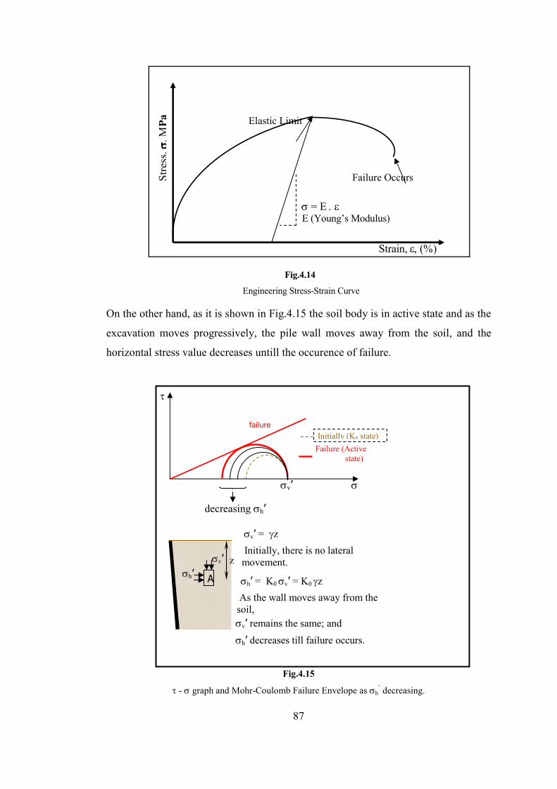
87

Fig.4.14

Engineering Stress-Strain Curve

On the other hand, as it is shown in Fig.4.15 the soil body is in active state and as the

excavation moves progressively, the pile wall moves away from the soil, and the

horizontal stress value decreases untill the occurence of failure.

Fig.4.15

τ - σ graph and Mohr-Coulomb Failure Envelope as σh’ decreasing.

τ

σ

failure

decreasing σh’

Initially (K0 state)

Failure (Active state)

σv’

A

σv’

σh’

z

As the wall moves away from the soil,

Initially, there is no lateral movement.

σv’ = γz

σh’ = K0 σv’ = K0 γz

σv’ remains the same; and

σh’ decreases till failure occurs.

Stress, σσ σσ

, , , , ΜPa

σ = E . ε

Strain, ε, (%)

E (Young’s Modulus)

Failure Occurs

Elastic Limit

88

The failure indications are presented according to Mohr-Coulomb model plastic points.

Plasticity is associated with the development of irreversible strains. Some Mohr-

Coulomb tension cut-off points occurred after the final excavation at the bottom of the

pile wall. Mohr-Coulomb plastic points occurred behind the excavation for the third

case which the anchorages are not applied can be clearly observed from the Fig. 4.16.

The circular failure zone can be revealed out from this result easily. The shown plastic

points seen in the figure are those Mohr-Coulomb plastic points which are fallen

above the failure envelope.

Fig.4.16

Plastic points occured after Case 3

As it is shown in Fig. 4.14 the plastic points follow circular failure zone at the upper

part of the excavation fall in the dumped fill zone and partly in the sandy clay zone.

These points show the plastic behavior as it is explained before and causes the soil body

to collapse.

Shear Failure Surface

89

Fig.4.17

Selected Stress-Points for Stress-Strain Values

σxx (σv’) and σyy (σh’ ) values are obtained from the analysis. The effective stresses

and strains are obtained from the selected points, distributed in the different material

cluster, are shown in Table 4.12 with the advance of excavation. The stress-strain

curve, with respect to defined points in the model geometry, are drawn Fig. 4.18. It

can be seen from this figure that the stress – strain behavior is quite different for each

soil cluster. It can be concluded from this result that the stiffer materials response

small values of strain for the same stress values. As it can be seen from the figure

that andesite shows very small strain values with respect to fill material for the same

stress. It is also possible to figure out that as the excavation takes progress the curve

slope decreases, which means that the stiffness of the soil changes with the

excavation.

A

B

C

D E

F

G H I

90

Table 4.12 Stress-Strain Values for selected points at each case

Case 1 Case 2 Case 3

Ef. Stress Tot. Strain Ef. Stress Tot. Strain

Ef. Stress

Tot. Strain

Cluster Point (x;y) (kN/m2) (%) (kN/m

2) (%) (kN/m

2) (%)

A (18,60 ; 23,30) 9,53 4,36 12,84 5,66 23,38 10,73

B (18,30 ; 22,40) 26,19 14,21 24,63 17,42 37,48 28,56 Fill

C (17,80 ; 18,10) 58,88 19,62 66,27 26,83 72,94 63,33

D (17,60 ;16,30) 83,91 0,43 86,33 0,67 91,44 0,71

E (18,40 ; 15,80) 106,58 1,02 110,04 1,05 119,68 1,09 Sandy Clay

F (17,20 ; 13,60) 114,26 1,68 118,64 1,71 124,94 1,73

G (18,30 ; 12,40) 117,49 0,051 121,72 0,052 133,77 0,062

H (19,10 ; 11,70) 126,65 0,056 131,43 0,053 135,46 0,063 Andesite

I (17,30 ; 10,20) 132,08 0,048 137,18 0,05 143,31 0,066

Case 4 Case 5 Case 6

Ef. Stress Tot. Strain Ef. Stress Tot. Strain

Ef. Stress

Tot. Strain

Cluster Point (x;y) (kN/m2) (%) (kN/m

2) (%) (kN/m

2) (%)

A (18,60 ; 23,30) 17,46 4,63 18,73 6,02 27,82 10,73

B (18,30 ; 22,40) 34,66 15,23 35,32 18,11 38,11 28,56 Fill

C (17,80 ; 18,10) 66,30 20,21 67,72 27,56 76,07 63,33

D (17,60 ;16,30) 88,76 1,12 92,13 0,79 96,60 0,81

E (18,40 ; 15,80) 113,07 1,38 115,25 1,26 120,32 1,29 Sandy Clay

F (17,20 ; 13,60) 118,16 1,73 122,45 1,84 126,54 1,83

G (18,30 ; 12,40) 122,55 0,076 124,07 0,072 134,76 0,072

H (19,10 ; 11,70) 133,47 0,081 136,69 0,078 141,61 0,083 Andesite

I (17,30 ; 10,20) 146,93 0,086 147,80 0,089 153,20 0,086

91

0

20

40

60

80

100

120

140

160

0 1 2 3 4 5 6

Total Strain (%)

Effective Stress (kN/m2)

Fig.4.18

Stress-Strain behavior of the clusters (after case 3)

It has to be stated that these values are calculated for case 1, case 2 and case 3 which

are the cases that no anchorages are applied. It is important to observe the soil and

pile behavior without anchorages in order to understand the anchored behavior and

the effects of anchorages on pile wall and soil body. After the application of the

anchorages the fill cluster has a low stress-strain with respect to the sandy clay and

andesite and the most of the Mohr-Coulomb points occured at this layer are not

observed. Fig.4.19 shows the decrement of the plastic points after the final

excavation stage with the application of anchors.

Andesite

Sandy Clay

Fill

92

Fig.4.19

Plastic Points occured after case 6

It can be noted that the amount of plastic stress points are less than the situation

(Case 1) without anchors. The effect of soil anchors are in good agreement with the

Mohr-Coulomb failure criteria. Applying of soil anchors gives a result of decrease in

plastic points which is also expected.

The occurred plastic points of the soil are at the slope near to the surface level. The

deformations at these points are irreversible. As it can be seen from this figure no

plastic points occurred along the anchor length. It is very important that the

deformations are in elastic limit at the anchor fixed length in case of the wall stability

as long as the fixed length grouted to the soil. Deformations are also very low at

anchor grout body.

The maximum horizontal displacement at the grout body is computed as 3,55 mm

which can be considered as low and in elastic limits. At this case some plastic points

occurred at the head of the fixed anchor length due to the prestress load. This can be

ignored due to the constraints of the Plaxis model. The grout body is modeled with

geotextile element and it is important to select the true element behavior and inserted

parameters. The FE analyses generally overestimate the soil and wall deflections but

93

appear to be in good agreement with the real behavior. It has to be considered that

there is no failure occurred during these excavations and anchoring stages in real

behavior but thanks to Plaxis the rather large deformations can be predicted in good

agreement with the real behavior. This helps to avoid extensive discussions about

permissible deformations during construction.

The same stress-strain relation is also observed for the cases with anchors. It can be

noted that with applying of anchors, an increase is observed at the effective stress

values. This is an expected situation due to the increase of horizontal stresses of the soil

behind the wall. As the soil cantilever deflection decreases due to the anchorage the

horizontal stresses shows higher values than the cases without anchor installation.

The strain values of the soil clusters is also increased due to the increase of the stress

values but as it can be noted from the table the strain values gives close results. A

comparison of stress – strain curves with the final case (6th Case) with and without

anchorage for fill soil cluster is shown in Fig. 4.20.

Fig.4.20

Comparison of stress-strain relation of fill layer with and without anchors

0

5

10

15

20

25

0 5 10 15 20

Total Strain (%)

Effective Stress (kN/m2)

Case 5

Case 4

Case 1

Case 2

Case 3

Case 6

Without Anchors

With Anchors

94

It can be seen from this figure that the anchored stress – strain behavior gives higher

stress values for almost same values of strain. It is quite understandable that as the

anchored wall lateral displacement decreases the soil body behind the the wall gives

higher stress values and the number of plastic Mohr-Coulomb points decreases as it is

explained from Fig.4.16 given before. The stress capacity of the soil is increased with

the applying of anchors.

Applying of anchors gives a higher stress-strain capacity for soil layers and it is quite

considerable for the fill layer. The Mohr-Coulomb points mostly occurred at fill layer

without anchors as it is stated before. In this case the fill layer shows a stiffer behavior

than the model without anchors and it is very obvious that the plastic points shows a

considerable decrease as it is shown in Fig.4.19 .

It can be seen from Fig.4.20 for case 3 the fill layer shows a failure but it is quite

considerable that for the case 6, the fill layer shows a stiff behavior, and no Mohr-

Coulomb points occurred for selected points which means that no failure observed for

these points for the same stress-strain values.

Fig.4.21 shows the principal effective stresses in the final situation. The passive stress

state beneath the bottom of the excavation is clearly visible. It can also be seen that

there are stress concentrations around the grout anchors.

95

Fig.4.21

Principal effective stresses at the final stage (Case 6)

4.7.5. Settlements at the surface behind pile wall

The FE analysis settlements are also in good agreement with the literature. Calculated

maximum settlement is 1,514 mm occurring 5,50 m behind the wall. It is also observed

that no settlement occurred at the selected points beneath the building which is also a

good agreement in a manner of the stability of the building.

The chart shown in Fig 4.22 represents the vertical displacement at point J which is

selected beneath the building. At the final excavation stage no vertical displacements

occurred as it can be seen from the chart.

Fig. 4.22 The subsidence at point J.

96

4.7.6. Anchor Forces

It is observed that the measured anchor forces are well estimated by FEM. Anchors are

manufactured and tested according to DIN 4125. A 100 mm borehole is derived into

the ground horizontally with an inclination of 15o. Anchor rods are inserted into these

boreholes with a 100 mm PVC pipe wrapped around and 8 m length of the anchor rods

are grouted to obtain the fixed anchor length.

Anchors are tested according to DIN 4125 up to 1,25 times of its service load which is

50 tons. After the pull out test these anchors are locked to a prestress load which is 30

tons. The service load of these anchors during their service life is 40 tons.

In Plaxis, anchors can be pre-stressed in a staged construction calculation. In such a

calculation the pre-stress force for a certain calculation phase can directly be given in

the anchor property window. The pre-stress force is not considered to be a material

property and is therefore not included in an anchor data set. At this situation anchor

pre-stress locking force is given as 30 tons which is about 300 kN. The prestress

force is entered as kN/m in Plaxis.

The table below shows the anchor forces of Plaxis results before and after prestressing

of anchors.

Table 4.13 Anchor Forces

Anchor Force (kN/m)

Before Prestressing

Anchor Force (kN/m)

After Prestressing

1st ROW 48,650 263,700

2nd ROW 20,720 277,900

3rd ROW 2,380 294,000

The tensile forces in the anchor rod were calculated as it is shown in the figure. Before

the last excavation step the prestressing in the anchor rod was 294 kN. Therefore some

drop at the values is calculated.

97

4.7.7. Safety Analysis

It is important to consider not only the final stability, but also the stability during the

construction. It is interesting to evaluate a global safety factor at this stage of the problem,

and also for other stages of construction.

In structural engineering, the safety factor is usually defined as the ratio of the collapse

load to the working load. For soil structures, however, this definition is not always useful.

For embankments, for example, most of the loading is caused by soil weight and an

increase in soil weight would not necessarily lead to collapse. Indeed, a slope of purely

frictional soil will not fail in a test in which the self weight of the soil is increased (like in a

centrifuge test). A more appropriate definition of the factor of safety is therefore:

quilibriumneededfore

bleimumavaila

S

SorSafetyFact max=

Where, S represents the shear strength. The ratio of the true strength to the computed

minimum strength required for equilibrium is the safety factor that is conventionally used

in soil mechanics. By introducing the standard coulomb condition, the safety factor is

obtained:

rnr

n

c

corSafetyFact

φσφσ

tan

tan

+

+=

Where c and φ are the input strength parameters and σn is the actual normal stress

component, 'the parameters cr and φr are reduced strength parameters that are just large

enough to maintain equilibrium. The principle described above is the basis of the method

of Phi-c-reduction that can be used in PLAXIS to calculate a global safety factor. In this

approach the cohesion and the tangent of the friction angle are reduced in the same

proportion:

Msfc

c

rr

Σ==φφ

tan

tan

98

The reduction of strength parameters is controlled by the total multiplier

ΣMsf. This parameter is increased in a stop-by-step procedure until failure occurs. The

safety factor is then defined as the value of ΣMsf at failure, provided that at failure a more

or less constant value is obtained for a number of successive load steps.

The Phi-c-reduction calculation option is only available in PLAXIS for Plastic

calculations of the Load advancement number of steps type.

The below table shows the ΣMsf values after each excavation stage and these

values and FEM results are compared with the values published in the literature for

similar excavations. It can be stated that the displacements are within expected

margins. For excavations in clay and clayey soil researchers agree on a factor of

safety against basal heave which is less than 1,5 – 2,0 can cause excessive

displacements. (Mana&Clough, 1981, Wong&Broms, 1989).

Table 4.14 – ΣΣΣΣMsf values at excavation stages

Case ΣΣΣΣMsf

1 2,181

2 1,478

3 1,167

4 3,808

5 3,983

6 3,377

The values for these six cases shows that the ΣMsf values with anchored cases are

higher than the ΣMsf values without anchorage. This is also an expected result for the

safety analysis procedure. This means that the anchored wall and the surrounding soil

shows more stabilized behavior. The pile wall and soil behavior are far more than

greater than the critical values and the displacements of the wall are within expected

limits. Case 3 seems to be the critical step which is not a construction practice but it is

modeled to observe the pile wall and soil behavior in a manner of understanding and

comparison of the anchored behavior.

99

4.7.8. Active & Passive Earth Pressures

The lateral earth pressure is investigated according to Rankine’s Active&Passive

Earth Pressure theory.

Total earth pressure distribution is calcualted due to the FEM analysis and Rankine’s

theory for excavation and is shown at figure below.

Fig.4.23

Active and Passive thrusts on the wall

KA and KP values for each soil part can be calculated with the given formulas below.

After the KA values be calculated Rankine’s horizontal Earth Pressure values are

calculated and compared with the FEM results and shown in Fig.4.24.

[σh’]passive

[σh’]active

H

h

PA=0.5 KAγγγγH2

PP=0.5 KPγγγγh2

KγH Kγh

)2/45(tansin1

sin-1 2 φφφ

−=+

=AK )2/45(tansin1

sin1 2 φφφ

+=−+

=PK

100

9

8

6

4

Elevation (m)

FEM

Calculated

10 30 60 90

Active Pressure on the Wall

(kN/m2)

20 40 50 70 80 Passive

Pressure on the Wall (kN/m2)

Computed active and passive earth pressure distributions behind the wall are shown in

Fig. 4.23. Rankine active earth pressure distribution is plotted on the same figure for

comparison. From the figure, it can be observed that computed and FEM earth

pressure values are so close.

The Table 4.15 given below shows the comparison of the minimum and maximum

FEM results and calculated Rankine results of the active and passive earth pressures on

the wall.

Fig. 4.24

Rankine and FEM result for active and passive earth pressure distribution

Table 4.15 Comparison of FEM and Rankine Results

Plaxis Results

(kN/m2)

Rankine Theory Results (kN/m2)

min. max. min. max.

Active -3,528 69,475 0,935 74,340

Passive -1,712 -19,657 -1,071 -17,136

101

4.7.9. Heave of the Soil in front of the Wall

Figure 4.25 shows the FEM results at the final excavation stage for the heave of the soil

in front of the wall respectively. Computed maximum heave is 8,1 mm occuring 9,8 m

in front of the wall at the final excavation level.

Fig. 4.25

Computed Heave in front of the Wall

These are expected results considering the magnitude of lateral wall deflection.

Maximum heave of the bottom is computed as 8,1 mm which occurs at a close point to

the middle of the excavation. As far as no field data available for settlements or heave

therefore the FEM results cannot be compared. However, the results seem acceptable

considering the dimensions of the excavation and the idealized soil profile.

Sandy Clay

Andesite

Distance from Wall (m)

0 3 6 9 12 15

hmax = 0,0081 m

Fill

102

CHAPTER V

RESULTS & DISCUSSION

The simplified model was used to predict the behavior of anchored piles and the

stress-strain behavior of the soil clusters during the anchor piled excavation. The 2D

finite element analyses and the case studies indicate a failure zone and Mohr –

Coulomb stress points behind the pile wall related to the excavation.

In this chapter the study results are discussed step by step and the following

conclusions are deducted.

5.1. Lateral Deflections of Pile Wall

The pile cap deformations are considered during this study and compared with different

cases. Plaxis results indicaste an inward cantilever deflection of 13,5 cm without anchors

and give an inward cantilever deflection of 10,9 cm with anchors. The effect of

anchorage is so clear that the lateral movement can be kept within permissible values.

Plaxis generally overestimates the lateral deflections and similar studies bring up same

conclusions. The magnitude of the pile cap displacements is rather small at Gazino

station excavation. The maximum pile cap deformation is measured as 8 mm for the

modeled section but there is a scatter in field measurements. Also, surveying

measurements contradict at some locations. It is important to use an inclinometer during

the measurement of pile displacements.

Morgenstern and Eisenstein, 1970 are stated that lateral earth stresses are computed

for a wall displacement toward excavation of 0,0025H, which is less than the

displacement necessary for the active state (H: Height of the Wall).

Plaxis results show compatible values with the 0,0025H value.

5.2. Stress – Strain Behavior

5.2.1. Non-Anchored Behavior

The behavior of the pile wall and the soil body is investigated during the excavation

stages without anchors. In case 3, all the excavations are completed but no anchors are

applied.

103

After the final excavation stage the soil body shows a failure zone from the top levels

of the fill layer to the bottom levels of the sandy clay layer. (Figure 4.14) Andesite

layer shows quite stiff behavior according to the fill and sandy clay layers. It can be

stated from these analysis the stiffer soils show small values of strain for the same

stress values. Due to the Mohr-Coulomb parameters of the soil layers (Young’s

Modulus of the soil is one of the most important parameter at this point) the failure

can be observed for fill layer when there is no failure at andesite layer for the same

stress-strain values.

5.2.2. Anchored Behavior

Applying of soil anchors gives a result of decrease in plastic points which is also

expected. The occurred plastic points of the soil are at the slope near to the surface

level. The deformations at these points are irreversible. The failure zone is shifted to

the top levels of the fill layer as it is shown in Figure 4.19 before. As less Mohr-

Coulomb failure points occurred after applying of anchors a comparison is made for

the fill layer and plotted out in Figure 20. It can be seen from Figure rr for almost

same or higher stress-strain values, the anchored behavior of the soil remains in

elastic limits and less plastic points observed. This can also be observed for the

sandy clay layer.

104

CHAPTER VI

CONCLUSION

As a result of the FEM analysis the following conclusions can be drawn:

1. All calculation phases are defined as Plastic calculations of the Load

advancement ultimate level type using Staged construction as Loading input and

standard settings for all other parameters.

2. The excavation of the station has typical cross sections and one of these sections

modelled in 2D by Plaxis.

3. As it is mentioned before, the pile cap deformations are considered during this

study and compared with different cases.

4. The use of the finite element method (Plaxis) reasonable estimates can be made

of the horizontal and vertical displacements of the anchored concrete piles with

prestressed anchors. Although the FEM results tend to overestimate the

displacements above the excavation level and at the pile cap it must be noted

that the magnitude of the displacements are rather small.

5. Plaxis results indicate an inward cantilever deflection of 13,5 cm without

anchors and give an inward cantilever deflection of 10,9 cm with anchors. The

effect of anchorage is so clear that the lateral movement can be kept within

permissible values. Plaxis generally overestimates the lateral deflections and

similar studies bring up same conclusions but thanks to Plaxis the rather large

deformations can be predicted in good agreement with the real behavior. This

helps to avoid extensive discussions about permissible deformations during

construction. The magnitude of the pile cap displacements is rather small at

Gazino station excavation. The maximum pile cap deformation is measured as 8

mm for the modeled section but there is a scatter in field measurements. Also,

surveying measurements contradict at some locations. It is important to use an

inclinometer during the measurement of pile displacements but there is no

inclinometers were present at the construction site.

105

6. The installation of the anchors is to be recommended for all retaining structures

in a manner of the stabilization of the structure and the lateral movements can be

kept under control. Their installation is simple and they are not very expensive

and they can be easily recuperated for future use on similar pile walls.

7. It has been experienced that the extent of soil investigations and laboratory

data are limited for the deep excavation studied. This introduced some

difficulties in idealizing the soil profile as well as deriving the soil

parameters. As a result, the success of the FEM analysis may be affected due

to this limitation.

8. The computed displacements, i.e. Lateral wall deflections, settlements and

bottom heave are usually compatible with the values reported at the literature at

similar excavations.

9. The stress – strain behavior of the soil with and without anchors gives quite

considerable results in a manner of applying ground anchors. The non-anchored

excavation gives a large failure zone and Mohr-Coulomb plastic points are mostly

occurred at the top levels of the fill layer and less to the bottom levels of the sandy clay

layer. No plastic points and failure observed at the andesite layer due to the high values

of Mohr-Coulomb parameters of the andesite layer. Applying of ground anchors gives

quite reasonable results for the fill and sandy clay layer. As the stress-strain behavior

observed it can noted that the soil body shows no failure when compared with the

behavior without anchors. Applying of ground anchors at andesite layer shows no

considerable change in a manner of the stability of the andesite layer. According to

these Plaxis results it can be recommended that the applying of ground anchors at these

layers is a preference and a design matter.

10. Considering the high values of factor of safety at the anchored behavior, the

effect of ground anchors is quite certain when it is compared with the factor of

safety values without anchors. This is also an expected result for the safety

analysis procedure. This means that the anchored wall and the surrounding soil

shows more stabilized behavior.

106

The pile wall and soil behavior are far more than greater than the critical values and

the displacements of the wall are within expected limits.

11. Considering the high values of factor of safety against basal heave, bottom

heave is not expected to be critical at both excavations. Unfortunately, there

are no field measurements related to the bottom heave. However, the

magnitude of the bottom heave in FEM analysis is rather small compatible

with the high factors of safety against basal heave.

12. When equivalent earth pressure diagrams derived from measured and

computed anchor loads are examined, it is observed that the measured anchor

loads are generally well estimated.

13. The importance of deriving reliable soil parameters for the FEM analysis is

very clear with this example. Without proper parameters derived from careful

field and laboratory testing, simulating the field conditions at site is very

difficult.

14. Overall, the pile wall has fulfilled its primary design requirements of supporting

Gazino station.

107

REFERENCES

Bienawski Z.T. (1984). Rock Mechanics Design in Mining and Tunneling. A.A. Balkema, 97-133. Bowles, J.E. (1988). Foundation Analysis and Design, McGraw-Hill, Singapore British Standard Code of practice for Ground anchorages, BS8081:1989. pages 6-9, 23-35. Carter, M. and Bentley, S.P., (1991), Correlations of soil properties, Pentech Press, London Clough, G.W. and Tsui, Y. Performance of tied-back walls in clay, Proceedings, American Society of Civil Engineers, Vol. 100, No. GT12, 1978, 1259-1274. Craig R.F. Soil Mechanics first edition 1974 second edition 1978. Das, B.M. (1984). Principles of Foundation Engineering, PWS Publishers, Boston Das, B.M. (1983). Advanced Soil Mechanics, McGraw-Hill, Singapore Hanna H. Thomas, (1982). Foundations in Tension “Ground Anchors”, Trans Tech Publications Series on Rock and Soil Mechanics Vol.6 pages 1-29, 377-398. Hobst L. and Zajic J. (1983). Anchoring in Rock and Soil, Elsevier Scientific Publishing Company pages 3-6, 378-381, 408-414, 444-453. Hoek E. And Brown E.T. (1980). Underground Excavations in Rock. Institution of Mining and Metallurgy, 527pp. Hong S.H., Lee F.H., Yong K.Y. Three dimensional Pile-Soil Interaction in Soldier Piled Excavations (2002). Computers and Geotechnics Paper.

108

ISRM, (1981). ISRM Suggested Methods: Rock Characterization, Testing and Monitoring. E.T. Brown (ed.), Pergamon Pres, London, 211 pp. Littlejohn G.S., (1997). Ground anchorages and anchored structures, Proceedings of the international conference organized by the Institute of Civil Engineers and held in London, UK, on 20-21 March 1997 pages 100-108, 244-251, 308-317. Lunne, T. , Robertson, P.K. and Powell J.J.M. (1997). Cone Penetration Testing in Geotechnical Practice, Chapman & Hall, London Morgenstern, N. R., and Eisenstein, Z. (1970). Methods of estimating lateral loads and deformations, Proc., ASCE Speciality Conf. on Lateral Stresses in the Ground and Design of Earth Retaining Structures, ASCE

NAVFAC DM-7.1 (1982). Soil Mechanics Design Manual Ordemir I. Pile Foundations (1984). METU Library Publications. Ordemir I. Foundation Engineering, (1984). METU Library Publications. Ostermayer, H. Construction, carrying behavior and creep characteristics of ground anchors. Proceedings, Conference on Diaphragm Walls and Anchorages, Institution of Civil Engineers, London, 1974, 141-151. Plaxis Bulletin issue 18/October 2005 4D Grouting Pressure Model of a Bored Tunnel in 3D Tunnel.

Plaxis Bulletin issue 17/March 2005 Control of Ground Movements for Multi Level-Anchored Diaphragm Wall during Excavation. Plaxis Bulletin issue 12/June 2002 Comparison of Mohr-Coulomb and Hardening Soil Material Models.

Plaxis Bulletin issue 11/September 2001 Practice 1 Cut and Cover Tunnel with Sheet Pile Walls used as Anchor Walls in Switzerland.

109

Plaxis Bulletin issue 10/March 2001 Column Vermeer on Single Anchored Retaining Walls.

Plaxis v8.2 Finite Element Code for Soil and Rock Analysis Plaxis v8.2 Reference Manuals Plaxis v8.2 Scientific Manuals Thornbury P. Foundation Engineering (1964). Widmann R. (1995). Anchors in Theory and Practice, Anker in Theorie und Praxis, Proceedings of the International Symposium on Anchors in Theory and Practice, Salzburg-Austria 9-10 October 1995, pages 77-87, 221-229, 293-303. Wong, I.H. , Poh, T.Y. and Chuah, H.L. (1997). Performance of excavations for depressed expressways in Singapore, Journal of Geotechnical and Geoenvironmenta

Engineering, ASCE, 123(7), 617-625. Xanthakos P. Petros, (1991). Ground anchors and anchored structures, A Wiley Interscience Publication pages 1-38, 366-403, 533-543, 557-563.