18 Use of Satellite Remote Sensing Data for Modeling...

18 Use of Satellite Remote Sensing Data for Modeling Carbon Emissions from Fires: A Perspective in North America

Zhanqing Li, Ji-Zhong Jin, Peng Gong and Ruiliang Pu

18.1 Introduction

Accurate accounting of carbon cycling is paramount to understanding and modeling global climate change. At present, a considerable amount of global carbon uptake (~2 Gt/year) remains unaccounted for in the carbon budget. It has been argued that the missing carbon may be absorbed in the terrestrial biomes of the Northern Hemisphere (Tans et al., 1990), in particular the temperate and boreal forests in North America (NA), which could account for the bulk (1.7 Gt/year) of the missing carbon (Fan et al., 1998). Fire is a driving factor controlling the carbon dynamics in NA, which affects both the sign and magnitude of the carbon budget (Stocks et al., 1996; Conard and Ivanova, 1997; Kasischke, 2000). According to the modeling results of Chen et al. (2000), boreal forests in NA have undergone tremendous fluctuations in its carbon budget over the last 200 years (Fig. 18.1). Around 1880 when widespread severe fires released a huge amount of carbon into the atmosphere, the forests were a very large source of carbon (~140 GtC/year) while around 1940, the forests became a very large sink of carbon (~200 GtC/year) due to fast forest regeneration that absorbed a large quantity of atmospheric carbon. The net carbon exchange is now so small that it is being debated whether the boreal forest is currently a sink (Chen et al., 2000) or a source (Kurz et al., 1995). The close correlation between the carbon budget and fire activity demonstrates the importance of the accurate estimation of carbon emissions from fires.

So far, the continental-scale estimates of carbon emission were made mainly for fires occurring over the forest ecosystem using ground-based fire datasets (French et al., 2000). Few attempts have been made employing remote sensing data from coast to coast. While ground-based data are valuable, they have certain limitations that can be overcome by remote sensing. Ground-based fire data are mainly restricted to total burned area with their quality and completeness varying from year to year and region to region. Remote sensing is capable of providing additional spatial and temporal fire information to improve fire emission estimations.

Zhanqing Li et al.

338

Figure 18.1 Model simulated time series of net carbon source/sink from boreal forests in the North America (left) and major disturbance factors (Chen et al., 2000)

In addition to burned area, remote sensing can provide “snapshots” of fire dynamics information (starting and ending dates and daily spread), and spatial heterogeneity (the degree of burning, fragmentation of burned scars, fuel type, biomass amount, etc.). On the other hand, remote sensing has its own limitations that do not allow providing all emission related parameters such as emission factor. Therefore, the best strategy is to combine conventional and satellite data to maximize their utility for fire emission estimation.

18.2 Carbon Emission Estimation

There is a simple mathematical formula to compute the emission of any chemical gas or particle species as originally proposed by Seiler and Crutzen (1980):

E BA FL FF EF (18.1)

where E is the emission of a gas (x) or particulate matter from fire (g)—(here, mainly for CO2); BA is burned area (ha); FL fuel loading (or density) (kg/ha); FF = fraction of fuel consumed (%); EF emission factor for gas species (x) or particulate matter (g/kg of fuel consumed). It has been, however, a daunting task to obtain any of these variables from ground, air-borne, or space-borne observations. Nearly none of them are trivial to derive from any observation platform, nor from modeling.

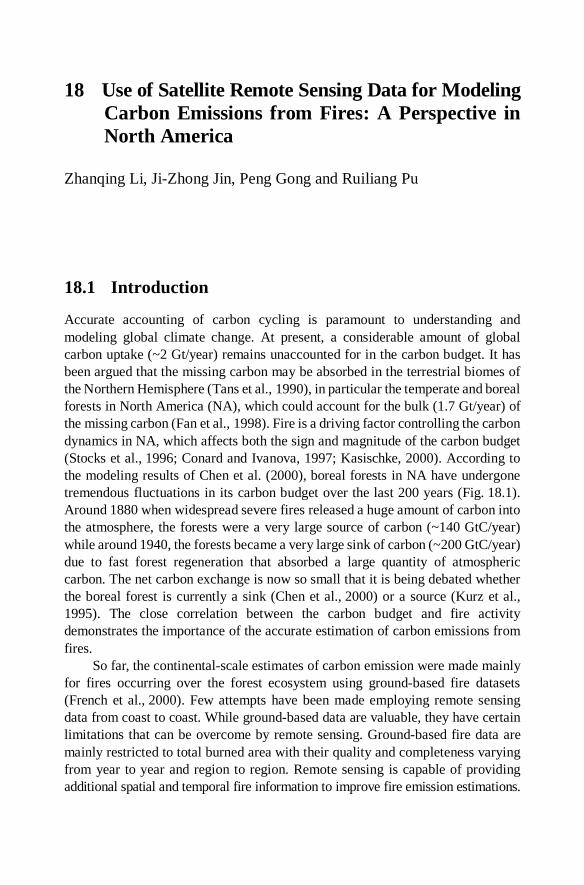
To effectively make use of a variety of spatial data in raster or vector formats, GIS-based emission modeling systems as is shown in Fig. 18.2 have

18 Use of Satellite Remote Sensing Data for Modeling Carbon …

339

been developed. For fire emission estimation, major fire emission attributes can be obtained from satellite and other sources as model inputs. They include burned area, degree of burning, fuel loading, above-ground and ground layer biomass amount, burning conditions and emission factors, etc.. Before running the system, the input data need to be acquired, edited and transformed as different attribute data layers. The system consists of several modular subsystems that simulate the burning processes. Some of the systems are based on the algorithms from the Forest Service First Order Fire Effects Model (FOFEM, Reinhardt, 1997) coded into Avenue (the ArcView scripting language) for implementation in the GIS.

The system needs to be able to use remote sensing data in combination with conventional data in order to enhance the estimation of carbon emissions and cycling.

Figure 18.2 Flowchart represents the Emission Estimation System (EES) modules. Boxes represent module components. Shading distinguishes modules from each other

18.3 Fire Emission Parameters and Modeling

18.3.1 Burned Area

There have been a large number of studies using satellite data to monitor and map fires around the globe. Recent reviews on fire detection, burned area mapping and fire observation systems/products may be found in Li et al. (2001a), Arino et al. (2001), and Grégoire et al. (2001), respectively.

Among all fire emission related factors, burned area can be inferred most accurately by satellite. This is because fires usually leave a distinct “footprint” that can be captured by satellite. Two types of “fire footprints” have been traced for fire

Zhanqing Li et al.

340

remote sensing, namely, the long-lived fire scars and short-lived fire hot spots. Fire scars may be measured by the drastic decrease in vegetation index such as the Normalized Difference Vegetation Index (NDVI) computed from reflectance in visible (VIS) and near infrared (NIR) channels:

(NIR VIS)NDVI(NIR VIS)

(18.2)

Numerous attempts have been reported to estimate burned areas based on changes in NDVI (Kasischke and French, 1995; Martin and Chuvieco, 1995; Li et al., 1997, 2000b). However, use of the NDVI alone tends to cause significant commission errors, since the NDVI decrease may be unrelated to fire and more related to drought, seasonal vegetation senescence, timber harvesting, image mis-registration, and cloud contamination. A further difficulty lies in the selection of effective thresholds for separating burns that are spatially and temporally variable (Fernandez et al., 1997).

One might composite all fire hot spots to obtain the burned area. As optical remote sensing of fires is only feasible under clear-sky conditions (Li et al., 2000a), an accumulation of fire hot spots may be substantially less than the actual area of burning, depending on cloud cover and frequency (Li et al., 2000b). To overcome these limitations, methods have been developed that combine synergistic information on fire hot spots and vegetation damage indicated by a vegetation index (Roy et al., 1999; Fraser et al., 2000a). A method named Hotspot and NDVI Differencing Synergy (HANDS) proposed by Fraser et al. (2000a) has a high degree of automation and self-adaptation(see Fig. 18.3). The

Figure 18.3 A simplified schematic of the HANDS method proposed by Fraser et al. (2000a) in generating burned area (right) by synergetic use of fire hot spot (left top) detected by the Li et al. (2000a) algorithm and vegetation index (left bottom)


341

principle of this method is to use hotspot locations to train spatially variable NDVI difference threshold, while changes in NDVI between two periods (before and after a fire, or on two anniversaries in two consecutive years) allow to eliminate false fire hot spots.

Using the fire detection algorithm of Li et al. (2000a) and the mapping algorithm of Fraser et al. (2000a), a long-term (1989 2000) daily 1-km fire product has been generated across the NA from the historical AVHRR archive (Pu et al., 2006, c.f. Fig. 18.4). Validations of the satellite mapped burned areas against fire polygons generated by air-borne surveillance showed a very close match (Li et al., 2003). Moreover, the satellite mapping method can pick up fires that were missed by the conventional method. This is especially the case over remote regions where fires are usually allowed to develop in their own natural course and so manual mapping is less complete. This and other validations (Fraser et al., 2000b; Fraser and Li, 2002) have revealed consistent high accuracy in mapping burned areas over forests.

Figure 18.4 Upper panels: nation-wide fire burned scars mapped from AVHRR data in 1989 and 2000. Such fire maps are available on a daily basis across NA continent. Lower left panel: comparison of fire burn scars mapped from satellite and the USDA Forest Service for the fires occurred in the western states in 2000 (Li et al., 2003)

Large errors are found in mapping fires over non-forest land (Csiszar et al., 2003). This has been a major problem for all satellite-based fire products using the mid-infrared channel of AVHRR around 3.7 µm, which is also a key channel for fire detection. The problem arises from channel saturation and the contribution

Zhanqing Li et al.

342

of solar reflection (Li et al., 2001a). Note that the main purpose of this channel was originally designed for mapping sea surface temperature during night overpass. The maximum detection limit is usually set around 320 K with a range of variation (Csiszar and Sullivan, 2002). This does not incur any problem unless exceptionally hot targets are detected such as fires or volcanoes that can readily saturate the channel. Were the saturation caused by hot targets alone, it would not be a problem so far as fire detection is concerned. Unfortunately, saturation may be caused by unusually large thermal emissions or solar reflection, or both. As illustrated in Li et al. (2001a), a scene of albedo over 20% in this wavelength can reflect enough solar radiation to saturate the channel. Although channel 3 is known to have a significant contribution of solar reflection in the mid-IR, none of the existing fire detection algorithms have taken it into consideration (Li et al., 2001a). This is partially because much attention has been paid to fires occurring over forests where reflectivity in that channel is very small ( 5%). For other natural scene types, surface reflectivity may be large, variable and difficult to obtain (Salisbury et al., 1991; Salisbury and D’Aria, 1994; Snyder et al., 1997), as shown in Fig. 18.5.

Figure 18.5 The emissivity of some natural materials (Salisbury et al., 1991). Note that emissivity is equal to 1 minus albedo

This inherent problem can be resolved/lessened by the MODIS sensor. MODIS has several advantages over the AVHRR for fire monitoring (Kaufman et al., 1998a; Justice et al., 2002; Roy et al., 2002; Ichoku et al., 2003; Kaufman et al., 2003; Li et al., 2004). First, the saturation limit for the MODIS 3.7 mchannel is much higher. Second, the MODIS products include estimates of surface emissivity at this and other IR channels. Use of the emissivity data and solar radiative transfer calculation, one can determine and subtract the contribution


343

of solar reflection from the total radiance measured at this channel so that the remaining signal is a true measure of thermal emission. Third, MODIS includes a longer mid-IR channel near 4 m where incoming solar radiation is much reduced. Fourth, MODIS has several additional channels that can greatly facilitate fire detection and mapping. One most useful channel is the shortwave (SW) IR channel around 1.6 m.

While NDVI has been widely used for mapping burned area, its signal may fade out quickly for regions where understory vegetation grows rapidly after fire. A vegetation index derived from a combination of SWIR channel around 1.6 mand NIR as was proposed by Kaufman and Remer (1994) has a long-lasting “memory” of burning:

NIR SWIRSWVINIR SWIR

(18.3)

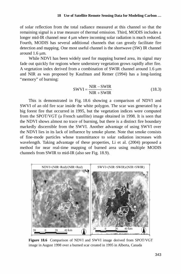
This is demonstrated in Fig. 18.6 showing a comparison of NDVI and SWVI of an old fire scar inside the white polygon. The scar was generated by a big forest fire that occurred in 1995, but the vegetation indices were computed from the SPOT/VGT (a French satellite) image obtained in 1998. It is seen that the NDVI shows almost no trace of burning, but there is a distinct fire boundary markedly discernible from the SWVI. Another advantage of using SWVI over the NDVI lies in its lack of influence by smoke plume. Note that smoke consists of fine-mode particles whose transmittance to solar radiation increases with wavelength. Taking advantage of these properties, Li et al. (2004) proposed a method for near real-time mapping of burned area using multiple MODIS channels from SWIR to mid-IR (also see Fig. 18.9).

Figure 18.6 Comparison of NDVI and SWVI image derived from SPOT/VGT image in August 1998 over a burned scar created in 1995 in Alberta, Canada

Zhanqing Li et al.

344

18.3.2 Spatial Fragmentation and Temporal Expansion of Burned Area

Burn fragmentation due to varying degrees of burning is next to total burned area in determining fire emissions. The methodology described based on AVHRR and MODIS sensors is adequate to delineate fire boundaries. However, a burning field generally shows very inhomogeneous distribution due to varying degrees of burning severity. Burn fragmentation is very important for estimating fire emissions. High-resolution data such as that from LANDSAT-7 TM is valuable for assessing fire severity (Michalek et al., 2000) and calibrating burned areas mapped by the coarse resolution data (Fraser et al., 2004).

Figure 18.7 shows a comparison of burned areas extracted from LANDSAT-5 TM and SPOT/VGT data for fires that occurred during May 1998 in Alberta, Canada. The outer burn perimeter derived using VGT data corresponds quite well to the TM boundary. However, as a result of the coarser resolution of VGT imagery (1 km), most interior small-scale unburned islands are mapped as being burnt. This leads to a systematic over-prediction of burnt area, and thus also the emission estimation. By double sampling a representative selection of fires with both TM and VGT data, a function of the two burned areas was derived that can be used to calibrate the coarse resolution burned area at a continental scale. The calibration coefficient may be parameterized by the change in a vegetation index before and after burning.

Figure 18.7 Left: Burned area derived from LANDSAT TM (white lines) and SPOT VGT (yellow lines) superimposed on a false color TM image. Right: comparison of burned areas estimated from fine-resolution TM data (20 m) and coarser resolution VGT data (1 km) (Fraser et al., 2004)


345

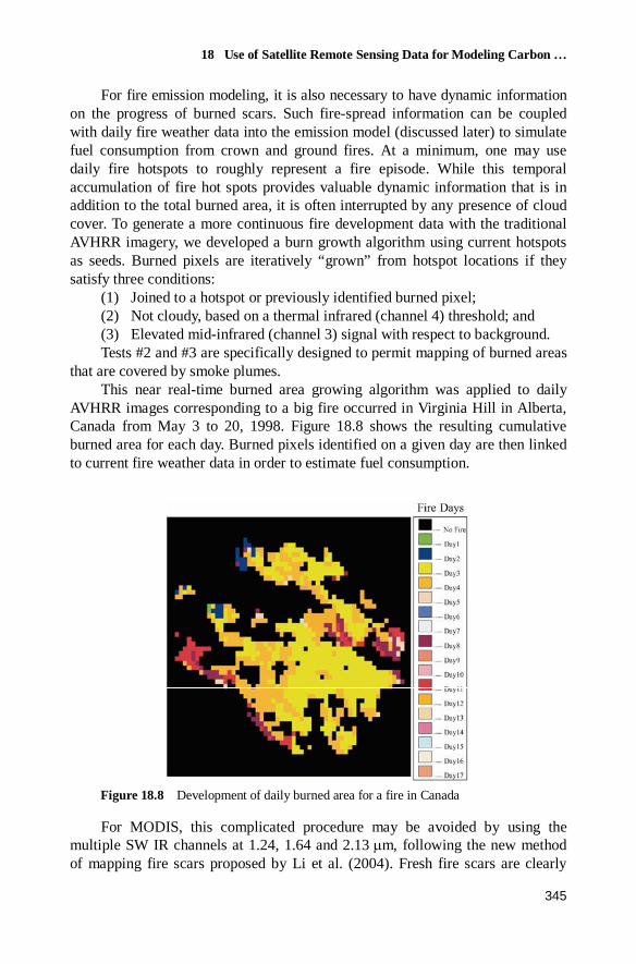
For fire emission modeling, it is also necessary to have dynamic information on the progress of burned scars. Such fire-spread information can be coupled with daily fire weather data into the emission model (discussed later) to simulate fuel consumption from crown and ground fires. At a minimum, one may use daily fire hotspots to roughly represent a fire episode. While this temporal accumulation of fire hot spots provides valuable dynamic information that is in addition to the total burned area, it is often interrupted by any presence of cloud cover. To generate a more continuous fire development data with the traditional AVHRR imagery, we developed a burn growth algorithm using current hotspots as seeds. Burned pixels are iteratively “grown” from hotspot locations if they satisfy three conditions:

(1) Joined to a hotspot or previously identified burned pixel; (2) Not cloudy, based on a thermal infrared (channel 4) threshold; and (3) Elevated mid-infrared (channel 3) signal with respect to background. Tests #2 and #3 are specifically designed to permit mapping of burned areas

that are covered by smoke plumes. This near real-time burned area growing algorithm was applied to daily

AVHRR images corresponding to a big fire occurred in Virginia Hill in Alberta, Canada from May 3 to 20, 1998. Figure 18.8 shows the resulting cumulative burned area for each day. Burned pixels identified on a given day are then linked to current fire weather data in order to estimate fuel consumption.

Figure 18.8 Development of daily burned area for a fire in Canada

For MODIS, this complicated procedure may be avoided by using the multiple SW IR channels at 1.24, 1.64 and 2.13 m, following the new method of mapping fire scars proposed by Li et al. (2004). Fresh fire scars are clearly

Zhanqing Li et al.

346

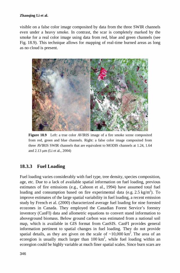
visible on a false color image composited by data from the three SWIR channels even under a heavy smoke. In contrast, the scar is completely marked by the smoke for a real color image using data from red, blue and green channels (see Fig. 18.9). This technique allows for mapping of real-time burned areas as long as no cloud is present.

Figure 18.9 Left: a true color AVIRIS image of a fire smoke scene composited from red, green and blue channels. Right: a false color image composited from three AVIRIS SWIR channels that are equivalent to MODIS channels at 1.24, 1.64 and 2.13 m (Li et al., 2004)

18.3.3 Fuel Loading

Fuel loading varies considerably with fuel type, tree density, species composition, age, etc. Due to a lack of available spatial information on fuel loading, previous estimates of fire emissions (e.g., Cahoon et al., 1994) have assumed total fuel loading and consumption based on fire experimental data (e.g. 2.5 kg/m2). To improve estimates of the large spatial variability in fuel loading, a recent emission study by French et al. (2000) characterized average fuel loading for nine forested ecozones in Canada. They employed the Canadian Forest Service’s forestry inventory (CanFI) data and allometric equations to convert stand information to aboveground biomass. Below ground carbon was estimated from a national soil map, which is available in GIS format from CanSIS. CanFI provides general information pertinent to spatial changes in fuel loading. They do not provide spatial details, as they are given on the scale of ~10,000 km2. The area of an ecoregion is usually much larger than 100 km2, while fuel loading within an ecoregion could be highly variable at much finer spatial scales. Since burn scars are


347

usually patchy and non-uniform, more spatially resolved fuel loading information would help improve estimates of fire emissions.

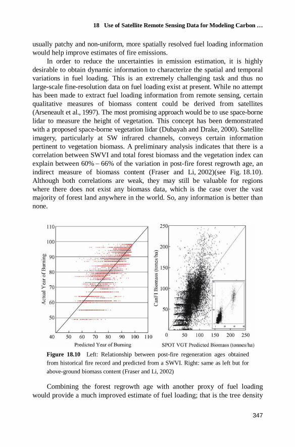
In order to reduce the uncertainties in emission estimation, it is highly desirable to obtain dynamic information to characterize the spatial and temporal variations in fuel loading. This is an extremely challenging task and thus no large-scale fine-resolution data on fuel loading exist at present. While no attempt has been made to extract fuel loading information from remote sensing, certain qualitative measures of biomass content could be derived from satellites (Arseneault et al., 1997). The most promising approach would be to use space-borne lidar to measure the height of vegetation. This concept has been demonstrated with a proposed space-borne vegetation lidar (Dubayah and Drake, 2000). Satellite imagery, particularly at SW infrared channels, conveys certain information pertinent to vegetation biomass. A preliminary analysis indicates that there is a correlation between SWVI and total forest biomass and the vegetation index can explain between 60% 66% of the variation in post-fire forest regrowth age, an indirect measure of biomass content (Fraser and Li, 2002)(see Fig. 18.10). Although both correlations are weak, they may still be valuable for regions where there does not exist any biomass data, which is the case over the vast majority of forest land anywhere in the world. So, any information is better than none.

Figure 18.10 Left: Relationship between post-fire regeneration ages obtained from historical fire record and predicted from a SWVI. Right: same as left but for above-ground biomass content (Fraser and Li, 2002)

Combining the forest regrowth age with another proxy of fuel loading would provide a much improved estimate of fuel loading; that is the tree density

Zhanqing Li et al.

348

or the fraction of forest cover inside a satellite pixel. Global distribution of the percentage of tree cover has been derived from 500 m resolution MODIS data (Hansen et al., 2002).

Use of the tree density information alone has proven valuable in estimating carbon emissions from the tropical deforestation and regrowth from 1980s to 1990s (DeFries et al., 2002). More accurate estimation of fuel loading would require a field survey to determine the average tree densities and diameters of different forest stands (Michalek et al., 2000) in order to better estimate above- ground biomass from the tree density data for different forest cover types. Allometric equations can be used to determine average tree biomass.

Despite these promising attributes from satellite, our ability to map fuel loads with satellite imagery is still very limited, as they are all concerned mainly with above-ground biomass. Below-ground biomass is even more difficult to estimate by any means, but it is very important for estimating the total emission from fires. Variations in the burning of organic soils account for a large portion of uncertainty in the estimates of emissions from forest fires, but not so for non-forest fires.

Average pre-burn ground layer biomass estimates are usually determined by collecting a number of ground layer profiles in each tree density class. The depths of different strata within the ground layer (e.g., litter, live moss, dead moss, fibric and humic soil) are measured at each profile. Samples of each stratum can be analyzed in the laboratory to determine bulk density and biomass.

While satellite remote sensing cannot be used to infer underground biomass directly, satellite observations of smoke loading integrated over the lifetime of burning could provide certain qualitative information of the biomass burned above and below ground, should the mode (smoldering or flaming) and temperature of burning be known (Kaufman et al., 1990). It is worthwhile to explore the relationship between burned biomass and smoke emissions. There are many ways to identify smoke from analysis of satellite imagery such as the threshold method, neural network method, pattern recognition method, etc.. Figure 18.11 presents an example of classification of smoke, cloud and clear land by applying the methods proposed by Li et al. (2001b) to AVHRR data. For MODIS, smoke can be much more easily identified from clouds whose reflectivity remains high for all solar channels using the combination of channels at short and longer wavelengths as illustrated in Fig. 18.9. Smoke emissions are generally proportional to smoke optical depths.

Aerosol optical depth has been retrieved from both sensors (Mishchenko et al., 1999; Kaufman et al., 2002). However, large uncertainties exist for smoke aerosol whose retrieval depend critically on aerosol absorption properties (Wong and Li, 2002). For smoke, absorption depends on fuel type and burning conditions. While this is a promising approach, little effort has been made, for it demands sizable resources to establish the relationship between the two quantities, as it


349

requires fire-by-fire analyses of total, above- and below-ground biomass amounts measured before, during and after burning.

Figure 18.11 A smoke image classified by a method of Li et al. (2001b) applied to the AVHRR data

18.3.4 Fuel Type

Fuel type is important for characterization of fire behavior, fuel loading and emission efficiency (Anderson, 1982). In NA, continental-scale fuel type data have been generated both in the US and Canada from land cover type (Eyre, 1980), forest inventory, above-ground and ground layer biomass survey, ecoregions, drainage classes, topography, and soil types (Bailey, 1998). In the US, fuel model and types are available from the National Fire Danger Rating System (NFDRS, http://www.fs.fed.us/land/ wfas/nfdr_map.htm) and the Forest Service Wildland Fire Assessment System (Burgan et al., 1998; Reinhardt et al., 1997). The conventional fuel type data are static and have coarse spatial resolution relative to other fire attributes extracted from satellite as elaborated above. As more refined and more reliable land cover classification data are now available from numerous satellite sensors (AVHRR, MODIS, TM/ETM ) (DeFries et al., 1998; Cihlar et al., 1999; Hansen et al., 2000), it is possible to generate continental-scale fuel type at high resolutions, together with low-resolution ground-based survey data on forest inventory, soil drainage class, and ecozone. An ecosystem map may help confirm the classified fuel types by examining whether they fall into a sound ecozone, such as the Terrestrial Ecozones and Ecoregions of Canada produced by

Zhanqing Li et al.

350

the Agriculture and Agri-Food Canada, Ecological Stratification Working Group (1996). A drainage map provides additional information that may be used to discriminate similar fuel types. After the various data sets are synthesized, a set of rules need to be established and applied by an expert system to classify the fuel types with multi-layer information. The criteria for the classification depend on the characteristics of fire behavior for a particular fuel type. The classification may follow a hierarchical structure in order to establish the relations between various input data sets and to organize the classification rules. Use of satellite data allows updating of the fuel type change due to biomass burning and other land cover and land use events.

18.3.5 Fraction of Fuels Consumed

The fraction of fuels consumed (FFC) by fire depends on fuel type, fuel loading, fuel moisture dictated by fire weather conditions, as well as the phase of combustion, i.e., smoldering or flaming. Studies on the estimation of fire emissions have either assumed a constant FF (Cahoon et al., 1994) or used temporally (monthly or seasonally) and spatially (regionally or provincially) averaged values (Vose et al., 1996). Cairns et al. (2000) assigned constants of above-ground biomass burned to four categories of forest. French et al. (2000) used a simple model to estimate a weighted fraction of biomass consumed for each year and ecozone based on annual area burned.

The spatial and temporal variations of FFC may be resolved by integrating various data sets, in particular the remote sensing data and the forest fire danger estimates provided by forest services on a daily basis. In Canada, such data are available from the Fire Weather Index (FWI) System (Van Wagner, 1987) and Fire Behavior Prediction (FBP) System (Forestry Canada Fire Danger Group, 1992). The systems have been operated during the fire season. The FWI system calculates fuel moisture codes and fire behavior indices based on daily weather conditions. The FBP system simulates fire behavior for each of the 16 fuel types based on the FWI indices, topography, and fuel type. The primary outputs of the FBP system are rate of spread, fuel consumption, and fire intensity. Total fuel consumption (TFC) includes surface fuel consumption (SFC) and crown fuel consumption (CFC). The moisture codes and indices of FWI system, fuel types, and topography determine how much surface fuel is consumed, whether a crown fire occurs, and what fraction of the crown fuel is consumed.

Figure 18.12 presents the flowchart of a fuel consumption and fire emissions modeling system developed based on the Canadian FWI and FBP modules. The system can make direct use of satellite-based products such as daily burned area and fuel type data. Therefore, the output can depict the spatial and temporal variation of fire emission. The system was run for estimating emissions from a big fire in Canada with the results presented in Fig. 18.13 (Li et al., 2000c). This


351

approach is better than the polygon-based model simulation that assumes homog- enous fuel distribution within a fire polygon.

Figure 18.12 A flowchart of a fuel consumption model for computing fraction of fuel consumed

Figure 18.13 Estimated fuel consumptions from surface (left) and tree crown fires for a big fires in Virginia fires in Alberta, Canada from May 3 20, 1995 (Li et al., 2000c)

This approach is similar to that of Cairns et al. (2000), but uses improved estimates of several key parameters from satellite: (1) more precise fire starting date, (2) fire ending date, (3) daily fire spread, and (4) burn severity and

Zhanqing Li et al.

352

fragmentation. For fire emissions modeling, fire weather is the primary factor dictating fuel consumption. Precipitation amount is an input of the system for determining fuel moisture. Information on vegetation moisture may also be extracted from NDVI or other vegetation indices from MODIS or AVHRR (Illera et al., 1996; Gonzalez-Alonso et al., 1997).

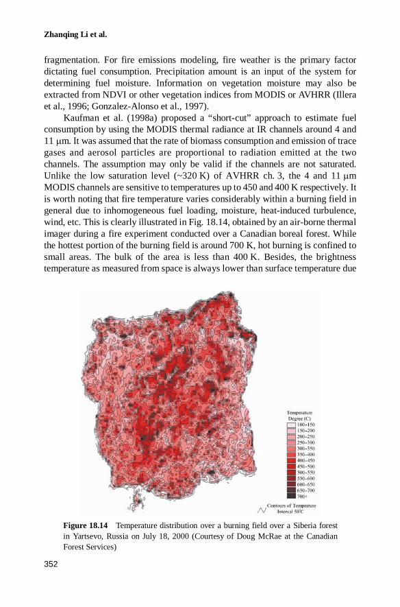
Kaufman et al. (1998a) proposed a “short-cut” approach to estimate fuel consumption by using the MODIS thermal radiance at IR channels around 4 and 11 m. It was assumed that the rate of biomass consumption and emission of trace gases and aerosol particles are proportional to radiation emitted at the two channels. The assumption may only be valid if the channels are not saturated. Unlike the low saturation level (~320 K) of AVHRR ch. 3, the 4 and 11 mMODIS channels are sensitive to temperatures up to 450 and 400 K respectively. It is worth noting that fire temperature varies considerably within a burning field in general due to inhomogeneous fuel loading, moisture, heat-induced turbulence, wind, etc. This is clearly illustrated in Fig. 18.14, obtained by an air-borne thermal imager during a fire experiment conducted over a Canadian boreal forest. While the hottest portion of the burning field is around 700 K, hot burning is confined to small areas. The bulk of the area is less than 400 K. Besides, the brightness temperature as measured from space is always lower than surface temperature due

Figure 18.14 Temperature distribution over a burning field over a Siberia forest in Yartsevo, Russia on July 18, 2000 (Courtesy of Doug McRae at the Canadian Forest Services)


353

to atmospheric attenuation and contribution of the atmospheric emission at much colder temperatures. As a result, the spatially integrated temperatures as registered by the MODIS sensor over a field of view of 1 km rarely exceed the saturation limits for ordinary wild fires. The relationship between the brightness temperatures at the two channels can serve as an indicator of relative contribution from smoldering and flaming fires to the total biomass consumption and evaluate their effect on the combustion efficiency and emissions (Kaufman et al., 1998a, 1998b).

Combustion efficiency may be measured as the fraction of carbon released from the biomass in the form of CO2 over the sum of CO2 and CO (Ward et al., 1996). To make this approach work, it requires extensive in-situ measurements of fire thermal energy, burned area and rate of emission of gases and particle matters in order to establish their relationships (Kaufman et al., 1998b). Yet, the relationship may be complex, as it is likely to change with vegetation types.

18.3.6 Emission Factor

Emission factors (EFs) are required to convert fuel consumption (kg) to gas and particulate emission yields (g). For large-scale fire emissions modeling, the EFs have normally been compiled from biomass burning experiments (Cofer et al., 1988; FIRESCAN Science Team, 1996; Goode et al., 2000). Comprehensive measurements have been made in some of the experiments that document the proportion of biomass burned, the combustion efficiency and the emission factors of CO2 and other trace gases. EFs were measured during the International Crown Fire Modeling Experiment for a jack pine with spruce understory fuel type (Cofer et al., 1998). The Boreal Forest Island Fire Experiment measured EFs for Scots Pine in Siberia (FIRESCAN Science Team, 1996). The experiments include reports on weather condition and vegetation characteristics (species, composition, fuel loading, fuel moisture content, etc.). Relationships between fire emission factors and burning and environmental conditions established from these experiments are valuable to better quantify the variation of emission factors (Hao et al., 1998; Susott and Ward, 1999; Yokelson et al., 1999).

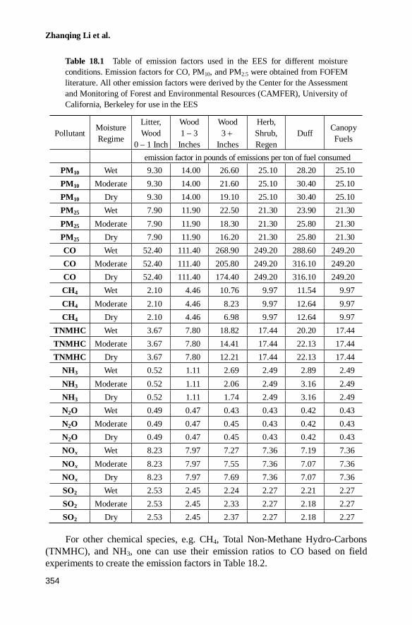
A comprehensive database of EFs was assembled from the literature based on results from fire experiments conducted in Canada and the United States. Table 18.1 lists the emission factors that we have compiled and used in the current version of our fire emission estimation system. A table in the FOFEM literature (Reinhardt et al., 1997) shows different combinations of combustion efficiencies for flaming and smoldering phases of combustion under varying moisture regimes. Ward and Hardy (1991) reported empirically derived equations for CO2 and CO as functions of combustion efficiency. Reinhardt et al. (1997) used the CO equation with the table of combustion efficiencies to create CO emission factors for different moisture regimes. These emission factors vary with moisture regime due to different ratios of flaming to smoldering combustion.

Zhanqing Li et al.

354

Table 18.1 Table of emission factors used in the EES for different moisture conditions. Emission factors for CO, PM10, and PM2.5 were obtained from FOFEM literature. All other emission factors were derived by the Center for the Assessment and Monitoring of Forest and Environmental Resources (CAMFER), University of California, Berkeley for use in the EES

Pollutant Moisture Regime

Litter, Wood

0 1 Inch

Wood 1 3

Inches

Wood 3

Inches

Herb, Shrub,Regen

Duff Canopy Fuels

emission factor in pounds of emissions per ton of fuel consumed PM10 Wet 9.30 14.00 26.60 25.10 28.20 25.10 PM10 Moderate 9.30 14.00 21.60 25.10 30.40 25.10 PM10 Dry 9.30 14.00 19.10 25.10 30.40 25.10 PM25 Wet 7.90 11.90 22.50 21.30 23.90 21.30 PM25 Moderate 7.90 11.90 18.30 21.30 25.80 21.30 PM25 Dry 7.90 11.90 16.20 21.30 25.80 21.30 CO Wet 52.40 111.40 268.90 249.20 288.60 249.20 CO Moderate 52.40 111.40 205.80 249.20 316.10 249.20 CO Dry 52.40 111.40 174.40 249.20 316.10 249.20 CH4 Wet 2.10 4.46 10.76 9.97 11.54 9.97 CH4 Moderate 2.10 4.46 8.23 9.97 12.64 9.97 CH4 Dry 2.10 4.46 6.98 9.97 12.64 9.97

TNMHC Wet 3.67 7.80 18.82 17.44 20.20 17.44 TNMHC Moderate 3.67 7.80 14.41 17.44 22.13 17.44 TNMHC Dry 3.67 7.80 12.21 17.44 22.13 17.44

NH3 Wet 0.52 1.11 2.69 2.49 2.89 2.49 NH3 Moderate 0.52 1.11 2.06 2.49 3.16 2.49 NH3 Dry 0.52 1.11 1.74 2.49 3.16 2.49 N2O Wet 0.49 0.47 0.43 0.43 0.42 0.43 N2O Moderate 0.49 0.47 0.45 0.43 0.42 0.43 N2O Dry 0.49 0.47 0.45 0.43 0.42 0.43 NOx Wet 8.23 7.97 7.27 7.36 7.19 7.36 NOx Moderate 8.23 7.97 7.55 7.36 7.07 7.36 NOx Dry 8.23 7.97 7.69 7.36 7.07 7.36 SO2 Wet 2.53 2.45 2.24 2.27 2.21 2.27 SO2 Moderate 2.53 2.45 2.33 2.27 2.18 2.27 SO2 Dry 2.53 2.45 2.37 2.27 2.18 2.27

For other chemical species, e.g. CH4, Total Non-Methane Hydro-Carbons (TNMHC), and NH3, one can use their emission ratios to CO based on field experiments to create the emission factors in Table 18.2.


355

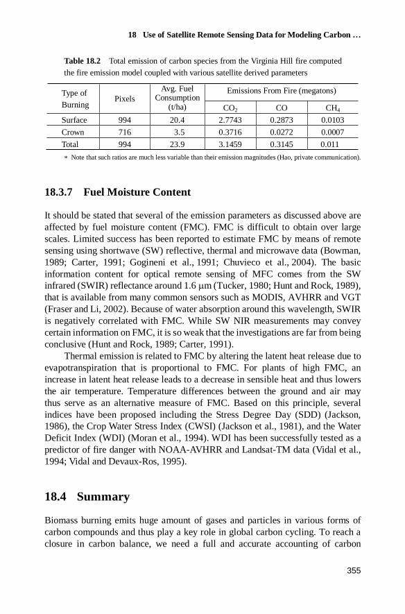
Table 18.2 Total emission of carbon species from the Virginia Hill fire computed the fire emission model coupled with various satellite derived parameters

Emissions From Fire (megatons) Type of Burning

Pixels Avg. Fuel

Consumption (t/ha) CO2 CO CH4

Surface 994 20.4 2.7743 0.2873 0.0103 Crown 716 3.5 0.3716 0.0272 0.0007 Total 994 23.9 3.1459 0.3145 0.011 * Note that such ratios are much less variable than their emission magnitudes (Hao, private communication).

18.3.7 Fuel Moisture Content

It should be stated that several of the emission parameters as discussed above are affected by fuel moisture content (FMC). FMC is difficult to obtain over large scales. Limited success has been reported to estimate FMC by means of remote sensing using shortwave (SW) reflective, thermal and microwave data (Bowman, 1989; Carter, 1991; Gogineni et al., 1991; Chuvieco et al., 2004). The basic information content for optical remote sensing of MFC comes from the SW infrared (SWIR) reflectance around 1.6 m (Tucker, 1980; Hunt and Rock, 1989), that is available from many common sensors such as MODIS, AVHRR and VGT (Fraser and Li, 2002). Because of water absorption around this wavelength, SWIR is negatively correlated with FMC. While SW NIR measurements may convey certain information on FMC, it is so weak that the investigations are far from being conclusive (Hunt and Rock, 1989; Carter, 1991).

Thermal emission is related to FMC by altering the latent heat release due to evapotranspiration that is proportional to FMC. For plants of high FMC, an increase in latent heat release leads to a decrease in sensible heat and thus lowers the air temperature. Temperature differences between the ground and air may thus serve as an alternative measure of FMC. Based on this principle, several indices have been proposed including the Stress Degree Day (SDD) (Jackson, 1986), the Crop Water Stress Index (CWSI) (Jackson et al., 1981), and the Water Deficit Index (WDI) (Moran et al., 1994). WDI has been successfully tested as a predictor of fire danger with NOAA-AVHRR and Landsat-TM data (Vidal et al., 1994; Vidal and Devaux-Ros, 1995).

18.4 Summary

Biomass burning emits huge amount of gases and particles in various forms of carbon compounds and thus play a key role in global carbon cycling. To reach a closure in carbon balance, we need a full and accurate accounting of carbon

Zhanqing Li et al.

356

emissions due to fire activities. Remote sensing is the only feasible means of monitoring fires around the globe. Maximum usage of satellite data is thus highly desired to achieve this goal. However, none of the emission related fire attributes are measured directly by any satellite sensors. Inversion algorithm and modeling are required to estimate fire emissions using satellite data.

This chapter provides an extensive review of remote sensing data and methods that could be brought to bear on fire emission estimation in terms of their information content, extraction method, strengths and limitations. These parameters include burned area, burning fragmentation and spreading, fuel loading, fraction of fuel consumed by fire, and emission factors for different gases. In general, satellites can provide good information on burned area by combined use of hot spot data together with changes in vegetation indices. Fire fragmentation and/or severity depend critically on satellite sensor resolution. For moderately coarse resolution data like MODIS and AVHRR, unburned fire islands inside the fire polygons provided by forest agencies may be singled out, but little can be gained concerning inhomogeneous degree of burning. Limited information may be extracted on fuel loading in terms of forest regrowth age, fraction of tree coverage by using a combination of measurements from several passive channels, especially NIR and SWIR data. Vegetation height detected by space-borne lidar may be linked to biomass content. Satellite-based land cover classification on continental scale may help refine fuel type classification. Determination of the fraction of fuel consumption (crown and surface) usually requires modeling, except for a short-cut approach that links radiation emission with fuel consumption.

References

Air Quality Policy on Agricultural Burning, Recommendation from the Agricultural Air Quality Task Force (AAQTF) to US Dept. of Agriculture, November 10, 1999

Anderson HE (1982) Aids to Determining Fuel Models for Estimating Fire Behavior. USDA Forest Service. General Technical Report INT 122

Arino O, Piccolini I, Kasischke E, Siegert F, Chuvieco E, Martin P, Li Z, Fraser HE, Stropplana D, Pereira J, Silva JMN, Roy D, Barbosa P (2001) Mapping of burned surfaces in vegetation fires, in Global and Regional Vegetation Fire Monitoring from Space, Planning and Coordinated International Effort (Eds. Ahern F, Goldammer JG, Justice C). pp 227 255

Arseneault D, Villeneuve N, Boismenu C, Leblanc Y, Deshaye J (1997) Estimating Lichen Biomass and Caribou Grazing on Wintering Grounds of Northern Quebec: an Application of Fire History and Landsat Data. Journal of Applied Ecology 34 (1): 65 78

Bailey RG (1998) Ecoregions: The Ecosystem Geography of the Oceans and Continents. Springer-Verlag, New York, 192 P


357

Bowman WD (1989) The relationship between leaf water status, gas exchange, and spectral reflectance in cotton leaves, Remote Sensing of Environ 30: 249 255

Burgan RE, Klaver RW, Klaver JM (1998) Fuel models and fire potential from satellite and surface observations. International Journal of Wildland Fire 8 (3): 159 170

Cahoon DR, Stocks BJ, Levine JS, Cofer WR, Pierson JM (1994) Satellite analysis of the severe 1987 forest fires in northern China and southeastern Siberia. Journal of Geophysical Research 99: 18,627 18,638

Cairns MA, Hao WM, Alvarado E, Haggerty PK (2000) Carbon emission from Spring 1998 fires in tropical Mexico. Proceedings of the International Conference on Tropical Forests and Climate Change: Status, Issues and Challenges. October 19 22, 1998, Manila, Philippines

Carter GA (1991) Primary and secondary effects of water content on the spectral reflectance of leaves. American J Botany 78: 916 924

Chen JM, Chen WJ, Liu J, Cihlar J, Gray S (2000) Annual carbon balance of Canada’s forest during 1895 1996. Global Biogeochemical Cycles 14: 839 850

Chuvieco E, Conalton RG (1988) Mapping and inventory of forest fires from digital processing of TM data. Geocarto International 4: 41 53

Chuvieco E, Vaughan P, Riano D, Cocero D (2004) Fire danger and fuel moisture content estimation from remotely sensed data. Proceedings of the Joint Fire Science Conference and Workshop. Boise, Idaho, June 15 17, 1999

Cihlar J, Beaubien J, Latifovic R, Simard G (1999) Land Cover of Canada 1995 Version 1.1. Digital data set documentation. Natural Resources Canada, Ottawa, Ontario

Clinton N, Gong P, Pu R (2003) Evaluation of wildfire mapping with NOAA/AVHRR data by land cover types and eco-regions in California. Submitted to Int. J. Wildland Fire, 2003

Cofer WR, Winstead EL, Stocks BJ, Goldammer JG, Cahoon DR (1998) Crown fire emissions of CO2, CO, H2, CH4, and TNMHC from a dense jack pine boreal forest fire. Geophysical Research Letters 25: 919 922

Cofer WR, Levine JS, Riggan PJ, Sebacher DI, Winstead EL, Shaw EF, Jr. Brass JA, Ambrosia VG (1988) Trace gas emission from a mid-latitude prescribed chaparral fire. Geophysical Research 93: 1,653 1,658

Conard SG, Ivanova GA (1997) Wildfire in Russian boreal forests—Potential impact f fire regime characteristics on emissions and global carbon balance estimates. Environ Pollut 98: 305 313

Csiszar I, Abdelgadir A, Li Z, Jin J, Fraser R, Hao W (2003) Interannual changes of active fire detectability in North America from long-term records of the Advanced Very High Resolution Radiometer. J Geophy Res 108(D2): 4075, doi: 10.1029/2001JD001373

Csiszar I, Sullivan J (2002) Recalculated pre-launch saturation temperatures of the AVHRR 3.7 micrometer sensors on board the TIROS-N to NOAA-14 satellites. International Journal of Remote Sensing 23: 5,271 5,276

DeFries RS, Hansen M, Townshend JRG, Sohlberg R (1998) Global land cover classification at 8 km spatial resolution. The use of training data derived from Landsat imagery in decision-tree classifiers. International Journal of Remote Sensing 19: 3,141 3,168

Zhanqing Li et al.

358

DeFries RS, Houghton RA, Hansen M, Field C, Skole DL, Townshend J (2002) for the 1980s and 90s. Proceedings of the National Academy of Sciences, 99 (22), Carbon emissions from tropical deforestation and regrowth based on satellite observations 14,256 14,261

Dubayah R, Drake J (2000) Lidar remote sensing for forestry applications. J Forestry 98: 44 46 Eyre FH (ed) (1980) Forest Cover Types of the United States and Canada. Society of American

Foresters Fan S, Gloor M, Mahlman J, Pacala S, Sarmieno J, Takahashi T, Tans P (1998) A large terrestrial

carbon sink in North America implied by atmospheric and oceanic carbon dioxide data and models. Science 282: 442 446

Fernandez A, Illera P, Casanova JL (1997) Automatic mapping of surfaces affected by forest fires in Spain using AVHRR NDVI composite image data. Remote Sens Environ 60: 153 162

FIRESCAN Science Team (1996) Fire in ecosystems of boreal Eurasia: The Bor Forest Island Fire Experiment fire research campaign, Asia-North (FIRESCAN). In Biomass Burning and Global Change Vol 2, pp 848 873. Edited by Levine JS, MIT Press, Cambridge, Massachusetts

Forestry Canada Fire Danger Group (1992) Development and structure of the Canadian Forest Fire Behavior Prediction System. Information Report ST-X-3, Forestry Canada

Fraser R, Li Z (2002) Estimating fire-related parameters in the boreal forest using SPOT VEGETATION. Rem Sens Environ 82: 95 110

Fraser R, Li Z, Cihlar J (2000a) Hotspot and NDVI differencing synergy: A new technique for burned area mapping over boreal forest. Rem Sens Environ 74: 362 375

Fraser R, Li Z, Landry R (2000b) SPOT VEGETATION for characterizing boreal forest fires. Int J Rem Sens 21: 3,525 3,532

Fraser RH, Hall RJ, Landry R, Landry T, Lynham T, Raymond D, Lee B, Li Z (2004) Validation and calibration of Canada-wide coarse-resolution satellite burned maps. Photogrammetric Engineering and Remote Sensing 70: 451 460

French NHF, Kasischke ES, Stocks BJ, Mudd JP, Martell DL, Lee BS (2000) Carbon release from fires in the North American boreal forest, pp 377 388. In: Fire, Climate Change and Carbon Cycling in the Boreal Forest (Eds. Kasischke ES, Stocks BJ). Ecological Studies Series, Springer-Verlag, New York

Garcia MJ, Caselles V (1991) Mapping burns and natural reforestation using thematic mapper data. Geocarto International 1: 31 37

Gogineni S, Ampe J, Budihardjo A (1991) Radar estimates of soil moisture over the Konza Prairie. Int J Rem Sens 12: 2,425 2,432

Gong P, Pu R et al. (2004a) Spatial and Temporal Distribution of Forest Fires in North America as Determined with NOAA/AVHRR Data. Being prepared for submitted

Gong P, Pu R et al. (2004b) A Report on Development of a Long-term (1989 2000) Inventory of Fire Burned Areas and Emissions of North America’s Boreal and Temperate Forests. Being prepared for submitted

Gonzalez-Alonso F, Cuevas JM, Casanova JL, Calle A, Illera P (1997) A forest fire risk assessment using NOAA AVHRR images in the Valencia area, eastern Spain. Int J Remote Sensing 18(10): 2,201 2,207


359

Goode JG, Yokelson RJ, Ward DE, Susott RA, Babbitt RE, Davies MA, Hao WM (2000) Measurements of excess O3, CO2, CO, CH4, C2H4, C2H2, HCN, NO, NH3, HCOOH, CH3COOH, HCHO, and CH3OH in 1997 Alaskan biomass burning plumes by airborne Fourier transform infrared spectroscopy (AFTIR). Journal of Geophysical Research 105(22): 147 166

Grégoire J-M, Cahoon DR, Stroppiana D, Li Z, Pinnock S, Eva H, Arino O, Rosaz JM, Csiszar I (2001) Forest fire monitoring and mapping for GOFC: current products and information networks based on NOAA-AVHRR, ERS-ATSR, and SPOT-VGT, in Global and Regional Vegetation Fire Monitoring from Space. Planning and Coordinated International Effort (Eds. Ahern F, Goldammer JG, Justice C), pp 105 124

Hansen MC, DeFries RS, Townshend JRG, Sohlberg R (2000) Global land cover classification at 1 km spatial resolution using a classification tree approach. International Journal of Remote Sensing 21: 1,331 1,364

Hansen MC, DeFries RS, Townshend J, Carroll M, Dimiceli C, Sohlberg R (2003) Global percent tree cover at a spatial resolution of 500 meters: First results of the MODIS Vegetation Continuous Fields algorithm. Earth Interactions Vol 7

Hao WM, Liu M.-H (1994) Spatial and temporal distribution of tropical biomass burning. Global Biogeochemical Cycling 8: 495 503

Hao WM, Ward DE, Olbu G, Baker SP (1996) Emissions of CO2, CO, and hydrocarbons from fires in diverse African savanna ecosystems. J Geophys Res 101: 23,577 23,584

Hao WM, DE Ward, Babbitt RE, Susott RA, Wang JS, Davies M, Baker SP (1998) Influences of weather and vegetation on biomass burning. Paper presented in the Joint International Symposium on Global Chemistry, Seattle, WA, August 19 25

Hunt ER, Rock BN (1989) Detection of changes in water content using near and middle-infrared reflectances. Rem Sens Environ 30: 43 54

Ichoku C, Kaufman Y, Giglio L, Li Z, Fraser RH, Jin J, Park B (2003) Comparative analysis of daytime fire detection algorithms using AVHRR data for the 1995 fire season in Canada: Perspective for MODIS. Int J Rem Sens 24: 1,669 1,690

Illera P, Fernandez A, Delgado JA (1996) Temporal evolution of the NDVI as an indicator of forest fire danger. Int J Remote Sensing 17(6): 1,093 1,105

Jackson RD, Idso SB, Reginato RJ, Pinter PJ (1981) Canopy temperature as a crop water stress indicator. Water Resources Res 17: 1,133 1,138

Jackson RD (1986) Remote sensing of biotic and abiotic plant stress. Ann Rev Phytopathology 24: 265 287

Justice CO, Giglio L, Korontzi S, Owens J, Morisette JT, Roy D, Descloitres J, Alleaume S, Petitcolin F, Kaufman Y (2002) The MODIS fire products. Remote Sensing of Environment 83: 244 262

Kasischke ES, French NHF (1995) Locating and estimating the areal extent of wildfires in Alaskan boreal forest using multiple-season AVHRR NDVI. Remote Sensing of Environment 51: 263 275

Kasischke ES, French NHF, Bourgeau-Chavez LL, Christensen NL (1995) Estimating release of carbon from 1990 and 1991 forest fires in Alaska. Journal of Geophysical Research 100: 2,491 2,951

Zhanqing Li et al.

360

Kasischke ES (2000) Boreal ecosystems in the global carbon cycle. pp 19 30. In: Fire, Climate Change and Carbon Cycling in the Boreal Forest (Eds. Kasischke ES, Stocks BJ). Ecological Studies Series, Springer-Verlag, New York

Kaufman YJ, Tucker CJ, Fung I (1990) Remote sensing of biomass burning in the tropics. J Geophys Res 95: 9,927 9,939

Kaufman YJ, Remer LA (1994) Detection of forests using mid-IR reflectance: an application for aerosol studies. IEEE Transactions on Geoscience and Remote Sensing 32: 672 683

Kaufman YJ, Justice C, Flynn L, Kandall J, Prins E, Ward DE, Menzel P, Setzer A (1998a) Monitoring Global Fires from EOS-MODIS. J Geophys Res 103 (32): 215 239

Kaufman YJ, Kleidman RG, King MD (1998b) SCAR-B Fires in the Tropics: properties and their remote sensing from EOS-MODIS. J Geophys Res 103 (31): 955 969

Kaufman YJ, Tanré D, Boucher O (2002) A satellite view of aerosols in the climate system. Nature 419: 215 223

Kaufman YJ, Ichoku C, Giglio L, Korontzi S, Chu DA, Hoa WM, Li R-R, Justice CO (2003) Fires and Smoke Observed from the Earth Observing System MODIS Instrument-Products, Validation, and Operational Use. International Journal of Remote Sensing 20: 1,031 1,038

Kurz WA, Apps MJ, Bekema SJ, Lekstrum T (1995) 20th century carbon budget of Canadian forests. Tellus (B) 47: 170 177

Li Z, Cihlar J, Moreau L, Huang F, Lee B (1997) Monitoring fire activities in the boreal ecosystem. J Geophy Res 102 (29): 611 624

Li Z, Nadon S, Cihlar J (2000a) Satellite detection of Canadian boreal forest fires: Development and application of an algorithm. Int J Rem Sens 21: 3,057 3,069

Li Z, Nadon S, Cihlar J, Stocks BJ (2000b) Satellite mapping of Canadian boreal forest fires: Evaluation and comparison and comparisons. Int J Rem Sens 21: 3,071 3,082

Li Z, Jin J-Z, Fraser RH (2000c) Mapping burning areas and estimating fire emissions over the Canadian boreal forest. Proceedings of the Joint Fire Science Conference and Workshop, Idaho, USA, June 15 17, 1999, Vol 2, pp 247 251

Li Z, Kaufman YJ, Ithoku C, Fraser R, Trishchenko A, Giglio L, Jin J, Yu X (2001a) A review of AVHRR-based active fire detection algorithms: Principles, limitations, and recomm- endations, in Global and Regional Vegetation Fire Monitoring from Space. Planning and Coordinated International Effort (Eds. Ahern F, Goldammer JG, Justice C), pp 199 225

Li Z, Khananian A, Fraser R, Cihlar J (2001b) Detecting smoke from boreal forest fires using neural network and threshold approaches applied to AVHRR imagery, IEEE Tran Geosci & Rem Sen 39: 1,859 1,870

Li Z, Fraser R, Jin J, Abuelgasim AA, Csiszar I, Gong P, Pu R, Hao W (2003) Evaluation of algorithms for fire detection and mapping across North America from satellite, J Geophys Res 108(D2): 4 076, doi: 10.1029/2001JD001377

Li R, Kaufman YJ, Hao WM, Salmon JM, Nordgren BL, Gao BC (2004) A technique for detecting burn scars using MODIS data, IEEE Trans Geosci Rem Sens, 42(6): 1,300 1,308

Martin MP, Chuvieco E (1995) Mapping and evaluation of burned land from multitemporal analysis of AVHRR NDVI images. EARSEL Adv Remote Sens 4: 7 13


361

Michalek JL, French NHF, Kasischke ES, Johnson RD, Colwell JE (2000) Using Landsat TM data to estimate carbon release from burned biomass in an Alaskan spruce forest complex. Int J Remote Sensing 21(2): 2,323 2,338

Mishchenko MI, Geogdzhayev IV, Cairns B, Rossow WB, Lacis AA (1999) Aerosol retrievals over the ocean by use of channels 1 and 2 AVHRR data: sensitivity analysis and preliminary results. Appl Optics 38: 7,325 7,341

Moran MS, Clarke TR, Inoue Y, Vidal A (1994) Estimating crop water deficit using the relation between surface-air temperature and spectral vegetation index. Rem Sens Environ 49: 246 263

Pu R, Gong P (2003) Determination of Burnt Scars Using Logistic Regression and Neural Network Techniques from a Single Post-Fire Landsat-7 ETM Image. Photogrammetric Engineering and Remote Sensing, 70(7): 841 850

Pu R, Li Z, Gong P, Fraser R, Csiszar I, Hao W, Kondragunta S, Weng F (2006) Development and Analysis of a 12-year Daily 1-km Forest Fire Dataset across North America from NOAA/AVHRR Data, Rem. Sens. Environ., in press

Reinhardt ED, Keane RE, Brown JK (1997) First Order Fire Effects Model: FOFEM 4.0, User’s Guide. USDA Forest Service. General Technical Report INT-GTR-344

Roy DP, Giglio L, Kendall JD, Justice CO (1999) Multi-temporal active-fire based scar detection algorithm. International Journal of Remote Sensing 20: 1,031 1,038

Roy DP, Lewis PE, Kendall J, Justice CO (2002) Burned area mapping using multi-temporal moderate spatial resolution data—a bi-direction reflection model-based expectation approach. Rem Sens Environ 83: 263 286

Salisbury JW, D’Aria DM (1994) Emissivity of terrestrial materials in the 3 5 mm atmospheric window. Rem Sens Environ 47: 345 361

Salisbury JW, Walter LS, Vergo N, D’Aria DM (1991) Infrared (2.1 25 m) spectra of minerals, The Johns Hopkins University Press, Baltimore, MD

Seiler W, Crutzen PJ (1980) Estimates of gross and net fluxes of carbon between the biosphere and atmosphere. Climate Change 2: 207 247

Snyder W, Wan Z, Zhang Y, Feng YZ (1997) Thermal infrared (3 14 m) bi-directional reflectance measurements of sands and soils. Rem Sens Environ 60: 101 109

Still CJ, Collatz GJ, Berry JA, DeFries RS (2003) The global distribution of C3 and C4 plants: Carbon Cycle Implications. Global Biogeochemical Cycles 17(1):1006, doi: 10.1029/ 2001GB001807

Stocks BJ, Lee BS, Martell DL (1996) Some potential carbon budget implications of fire management in the boreal forest. In: Forest ecosystems, Forest management and the global carbon cycle (eds Apps MJ, Price DJ). NATO ASI Series, Springer-Verlag, Berlin, pp 90 96

Susott RA, Ward DE (1999) Ward, Smoke emission from ponderosa pine fuels exposed to a variety of fire histories and site preparation treatments. Final Report submitted to Arizona National Forests

Tans PP, Fung IY, Takahashi T (1990) Observational constrains of the global atmospheric CO2

budget. Science 247: 1,431 1,438

Zhanqing Li et al.

362

Tucker CJ (1980) Remote sensing of leaf water content in the near infrared. Rem Sens Environ 10: 23 32

Van der Werf GR, Randerson JT, Collatz GJ, Giglio L, et al. (2003) Continental-scale partitioning of fire emissions during the 1997 to 2001 El Nino/La Nina period. Science 303: 73 76

Van Wagner CE (1987) Development and structure of the Canadian forest fire weather index system. Canadian Forestry Service, Forestry Technical Report 35, Ottawa

Vidal A, Pinglo F, Durand H, Devaux-Ros C, Maillet A (1994) Evaluation of a temporal fire risk index in Mediterranean forest from NOAA thermal IR. Rem Sens Environ 49: 296 303

Vidal A, Devaux-Ros C (1995) Evaluating forest fire hazard with a Landsat TM derived water stress index. Agricul Forest Meteor 77: 207 224

Vose JM, Swank WT, Geron CD, Major AE (1996) Emissions from forest burning in the Southern United States: application of a model determining spatial and temporal fire variation. Biomass Burning and Global Change, Vol 2 edited by Levine JS, The MIT Press, Cambridge, Massachusetts, London, England, 1996

Wan Z, Li Z (1997) A physics-based algorithm for retrieving land surface emissivity and temperature from EOS/MODIS Data. IEEE Trans Geosci Rem Sens 35: 980 996

Ward DE, Hardy CC (1991) Smoke Emissions from Wildland Fires. Environment International 17: 117 134

Ward DE, Hao WM, Susott RA, Babbitt R, Shea RW, Kauffman JB, Justice CO (1996) Effect of fuel composition on combustion efficiency and emission factors for African savanna ecosystems. J Geophy Res 101(23): 569 576

White JD, Ryan KC, Key CC, Running SW (1996) Remote sensing of forest fire severity and vegetation recovery. Int J Wildland Fire 6: 125 136

Wong J, Li Z (2002) Retrieval of optical depth for heavy smoke aerosol plumes: uncertainties and sensitivities to the optical properties. J Atmos Sci 59: 250 261

Yokelson RJ, Goode JG, Bertschi I, Susott RA, Babbitt RE, Ward DE, Hao WM, Wade DD, Griffith DWT (1999) Emissions of formaldehyde, acetic acid, methanol, and other trace gases from biomass fires in North Carolina measured by airborne fourier transform infrared spectroscopy (AFTIR). J Geophy Res, in press

18 Use of Satellite Remote Sensing Data for Modeling...

Documents

Transcript of 18 Use of Satellite Remote Sensing Data for Modeling...