1.73

0.78

1.25

0.03

2.75

BACKGROUND PAPER

CREDIT SUPPLY AND PRODUCTIVITY GROWTH

FRANCESCO MANARESI AND NICOLA PIERRI

Credit Supply and Productivity Growth

Francesco Manaresi∗ Nicola Pierri§

November 2017

Abstract

We study the impact of bank credit supply on firm output and productivity. Exploiting a

matched firm-bank database, covering all credit relationships of Italian corporations over more

than a decade, we measure idiosyncratic supply-side shocks to firm credit availability. With this,

we estimate a production model augmented with financial frictions and show that an expansion

of credit supply leads firms to increase both their inputs and their value added and revenues for a

given level of inputs. Our estimates imply that a credit crunch will be followed by a productivity

slowdown, as experienced by most OECD countries after the Great Recession. Quantitatively,

the credit contraction between 2007 and 2009 can account for about a quarter of the observed

decline in Italian total factor productivity growth. Results are robust to an alternative measure

of credit supply shock that uses the 2007-2008 interbank market freeze as a natural experiment to

control for assortative matching between borrowers and lenders. Finally, we investigate possible

channels: access to credit fosters IT-adoption, innovation, exporting, and adoption of superior

management practices.

∗Bank of Italy - francesco.manaresi@bancaditalia.it§Stanford University - pierri@stanford.edu

We thank Nick Bloom, Tim Bresnahan, Liran Einav, and Matt Gentzkow for invaluable advice. We thank, for theirinsightful comments, Shai Bernstein, Barbara Biasi, Matteo Bugamelli, Rodrigo Carril Francesca Carta, EmanueleColonnelli, Han Hong, Pete Klenow, Ben Klopack, Simone Lenzu, Matteo Leombroni, Andrea Linarello, FrancescaLotti, Davide Malacrino, Petra Persson, Luigi Pistaferri, Paolo Sestito, Joshua Rauh, Luca Riva, Cian Ruane, EnricoSette, Pietro Tebaldi, and all participants in the Stanford IO workshop, Stanford applied economics seminar (Fall2015, Winter 2017, and Fall 2017), Second Bay Area Labor and Public conference (Fall 2015), seminars at Bankof Italy (Fall 2015 and Summer 2017), the Brown Bag Seminars at the Italian Treasury Department (Spring 2017),and the 13th CompNet Annual Conference (Summer 2017). Francesco Manaresi developed part of this project whilevisiting the Bank for International Settlement under the Central Bank Research Fellowship program. Nicola Pierrigratefully acknowledges financial support from the Bank of Italy through the Bonaldo Stringher scholarship, fromThe Europe Center at Stanford University through the Graduate Student Grant Competition, and from the Gale andSteve Kohlhagen Fellowship in Economics through a grant to the Stanford Institute for Economic Policy Research.All errors remain our sole responsibility. The views expressed by the authors do not necessarily reflect those of theBank of Italy.

JEL Classification: D22, D24, G21

Keywords: Credit Supply; Productivity; Export; Management; IT adoption

1 Introduction

Does lenders’ credit supply affect borrower firms’ productivity and, if so, how?

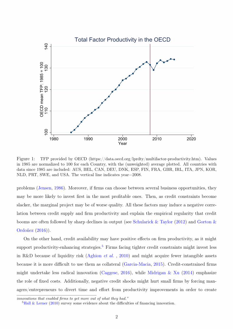
Aggregate productivity growth has declined in most OECD economies over the last decade, as

illustrated by figure 1. While financial crises are found to induce strong and persistent recessions,1

it is still an open question whether credit supply (or lack thereof) played a major role in generating

(and/or sustaining) this productivity slowdown.2

In this paper, we estimate the effect of idiosyncratic changes in the credit supply faced by Italian

firms on their total factor productivity (TFP) growth. We focus on Italy because of the availability of

detailed loan- and firm-level data on credit, inputs, and output. Khwaja & Mian (2008), Chodorow-

Reich (2013), and Amiti & Weinstein (2017) exploit lender-borrower connections to provide evidence

that negative bank shocks diminish credit supplied to borrowing firms and constrain those firms’

investment and employment.3 This paper extends the previous literature by looking at the impact

of credit on productivity and by tracing its channels.

The sign of the causal relation between availability of external finance and productivity is theo-

retically and empirically ambiguous. Standard models of financial frictions assume that agents have

an exogenous productivity, implying that credit constraints affect output only via reductions in the

amount of capital used in production. Richer models can generate either a negative or a positive

relationship. On the one hand, being forced to operate with fewer resources might spur innovation

(Field, 2003)4 and abundance might induce managers to stint their efforts or might aggravate agency1Several authors found that financial crises, and the Great Recession in particular, are different than other reces-

sions. See, for instance, Cerra & Saxena (2008), Reinhart & Rogoff (2009), Reinhart & Rogoff (2014), Jordà et al.(2013), and Oulton & Sebastiá-Barriel (2013). A contrasting view is expressed by Stock & Watson (2012).

2Fernald et al. (2017) document that the disappointing recovery of output after the Great Recession in the USis mainly due to low TFP dynamics, although they find it implausible that this is generated by financial shocks.Alternative explanations for the productivity slowdown are low business dynamism (e.g,. Decker et al. (2014) andDavis & Haltiwanger (2014)), mismeasurement of digital goods (e.g. Mokyr (2014), Feldstein (2015), Byrne et al.(2016)), slowdown of technological progress (e.g. Gordon (2016), Gordon et al. (2015), Bloom et al. (2016), Cetteet al. (2016)), and weak demand conditions (Anzoategui et al. , 2016). Additionally, Gopinath et al. (2017) and Cetteet al. (2016) argue that low interest rates have triggered unfavorable resource reallocations in southern Europe. Adleret al. (2017) argue for the interaction of several factors, from greater uncertainty to an aging workforce. Focusing onItaly, Hall et al. (2008) underline the lack of product innovation as a pre-crisis productivity problem.

3See also Bentolila et al. (2013), Greenstone et al. (2014), Cingano et al. (2016), and Bottero et al. (2015).4He documents that the years after the Great Depression were the most technologically progressive decade of

modern American History. In particular, he states: “In other sectors, for example railroads, the disruptions of financialintermediation and very low levels of capital formation associated with the downturn fostered a search for organizational

1

100

110

120

130

140

OEC

D m

ean

TFP:

198

5 =

100

1980 1990 2000 2010 2020Year

Total Factor Productivity in the OECD

Figure 1: TFP provided by OECD (https://data.oecd.org/lprdty/multifactor-productivity.htm). Valuesin 1985 are normalized to 100 for each Country, with the (unweighted) average plotted. All countries withdata since 1985 are included: AUS, BEL, CAN, DEU, DNK, ESP, FIN, FRA, GBR, IRL, ITA, JPN, KOR,NLD, PRT, SWE, and USA. The vertical line indicates year=2008.

problems (Jensen, 1986). Moreover, if firms can choose between several business opportunities, they

may be more likely to invest first in the most profitable ones. Then, as credit constraints become

slacker, the marginal project may be of worse quality. All these factors may induce a negative corre-

lation between credit supply and firm productivity and explain the empirical regularity that credit

booms are often followed by sharp declines in output (see Schularick & Taylor (2012) and Gorton &

Ordoñez (2016)).

On the other hand, credit availability may have positive effects on firm productivity, as it might

support productivity-enhancing strategies.5 Firms facing tighter credit constraints might invest less

in R&D because of liquidity risk (Aghion et al. , 2010) and might acquire fewer intangible assets

because it is more difficult to use them as collateral (Garcia-Macia, 2015). Credit-constrained firms

might undertake less radical innovation (Caggese, 2016), while Midrigan & Xu (2014) emphasize

the role of fixed costs. Additionally, negative credit shocks might hurt small firms by forcing man-

agers/entrepreneurs to divert time and effort from productivity improvements in order to create

innovations that enabled firms to get more out of what they had.”5Hall & Lerner (2010) survey some evidence about the difficulties of financing innovation.

2

relationships with new lenders (“managerial inattention”).

We contribute to the relevant literature on four dimensions. First, we combine firm-bank matched

data on credit granted by all financial intermediaries to all Italian incorporated firms over the period

1997-2013, with detailed balance-sheet information for a large sample of around 70 thousands firms,

to provide a complete picture of firm access to bank credit together with high-quality data on inputs

acquisition and output production for both large and small firms. Importantly, we are in the position

to credibly study firm-level financial constraints without limiting our analysis to syndicated loans or

public companies.

Second, we identify idiosyncratic credit supply shocks by exploiting two alternative empirical

strategies: one based on bank-firm relationships and the other on a natural experiment. Unlike

previous empirical studies on the link between finance and productivity, ours does not rely on self-

reported measures of credit constraints, (potentially endogenous) proxies of financial strength, or

local and industry-specific shocks (which might correlate with demand/technology dynamics).6

Our main empirical strategy decomposes the growth rate of credit of each bank-firm pair into

firm-year and bank-year components. The bank-year component reveals how different banks change

the quantity of credit granted to the same firm and it captures shocks to bank supply. This additive

decomposition, closely related to the ones developed by Amiti & Weinstein (2017) and Greenstone

et al. (2014), rests on assumptions related to the matching between banks and firms and the structure

of substitution/complementarity between lenders. We provide novel tests for these hypotheses.

To aggregate bank-specific credit supply shocks at the firm level, we exploit the stickiness of

bank-firm relations. Because of relationship lending, one lender’s expansion or contraction of credit

disproportionally affects its existing borrowers. As a result, two firms serving the same market might

experience different shocks to their ability to finance their operations because they have pre-existing

credit relations with different lenders.7 We therefore average bank shocks at the firm level, using

lagged credit shares as weights, to obtain a firm-specific credit supply shock. These shocks allow

us to study the effect of credit on firm output and productivity both in “normal times” and during

recessions.

Quantitatively, we find that a 1% increase in credit granted raises value-added TFP growth by6Like us, Huber (2017) examines the impact of credit supply on firms, using the lending contraction of a German

bank to undertake a thorough estimation of the impact on output and employment and showing large negative impacts.He does not, however, look at total factor productivity, which is the focus of this paper. He does have a regression,column (3) in Table VI of his paper, on labor productivity (value added per worker), but provides evidence regardingthe declining capital share and/or material inputs rather than declining TFP.

7The relevance of this phenomenon has been documented in several countries, including the US (Chodorow-Reich,2013), Italy (Sette & Gobbi, 2015), Spain (Jiménez & Ongena, 2012) and Pakistan (Khwaja & Mian, 2008).

3

around 0.1% and revenue TFP growth by 0.02-0.03%.8 During the financial crisis of 2007-2009, credit

growth shrank by around 12%: our estimates imply that a similar supply-driven credit crunch would

have induced between 12.5% and 30% of the average drop in firm TFP experienced by Italian firms

during that period. The effect of credit on TFP growth lasts up to two years and does not revert

afterwards, so that the impact on TFP is persistent over time and can partly explain the sluggish

productivity growth after the financial crisis. Large firms and firms with more lending relations, which

are probably more able to substitute away from contracting lenders, are largely unaffected by credit

supply. Effects are stronger in sectors where bank credit is more important; that is, manufacturing

and industries characterized by higher leverage. Our results imply that a credit crunch can generate

a productivity slowdown by depressing firm-level TFP. This effect may persist for several years.

To rule out the possibility that results are driven either by assortative matching between firms and

banks or other confounding factors or by some forms of reverse causality, we use a second empirical

strategy, which exploits the freeze of the interbank market in 2007-2008 as a natural experiment.

This shock affected Italian banks differently (and unexpectedly) according to their pre-crisis reliance

on this source of funding.9 We show that firms which the credit crunch hit harder through their

lenders experienced lower growth rate of productivity afterwards. Firm exposure to the interbank

market shock is found to be uncorrelated with pre-crisis growth potential and sensitivity to business

cycle. This alternative identification strategy confirms the causal link between credit supply and

productivity. Its estimated magnitude is significantly larger than the baseline estimates, suggesting

that the productivity effects are stronger during financial turmoil.

Third, we argue that the standard production function estimation methods would not allow one

to identify the causal effect of credit supply on productivity (see De Loecker (2013) for a conceptually

analogous case regarding the effect of exporting on efficiency). Therefore, we enrich the production

function estimation by allowing for heterogeneous credit constraints affecting both input acquisition

and productivity dynamics.10

8Since we do not observe firm-level output prices, productivity is the amount of revenues or value added (not thequantity of goods) generated for a given amount of inputs. In section 3.2, we clarify our terminology in relationto previous literature. We refer to the residuals of a production function as “revenue productivity” when output ismeasured by (log) net revenues and as “value added productivity” when output is measured by (log) value added.Measures of productivity estimated with revenues and quantities are usually found to be highly correlated.

9Cingano et al. (2016) show that firms that in 2006 were borrowing from banks more reliant on the interbankmarket experienced a stronger credit crunch, and that this, in turn, reduced investments.

10 We build on the literature on estimation of the production function with control functions: Olley & Pakes (1996),Levinsohn & Petrin (2003), Ackerberg et al. (2015), De Loecker & Warzynski (2012), De Loecker (2011), De Loecker& Scott (2016), Gandhi et al. (2011). In particular, Shenoy (2017) studies estimation of the production function whenfirms face heterogeneous and unobservable constraints that distort input acquisition but not productivity. Ferrando& Ruggieri (2015) and Peters et al. (2017a) are also related to our paper, since they estimate a production functionand allow firm financial strength to affect productivity dynamics.

4

Fourth, we augment our dataset with information from administrative and survey-based sources

in order to show that several productivity-enhancing activities, such as R&D, patenting, export,

innovation, IT-adoption, and adoption of superior management practices, are stimulated by credit

availability. These strategies increase productivity both in the short-run (e.g., IT-adoption) and in

the long-run (e.g., R&D). Therefore, their sensitivity to credit can explain the immediate effect of

credit supply shock on TFP and also suggests that there are additional effects over a longer horizon.

Finally, we discuss some indirect evidence consistent with the “managerial inattention” hypothesis.

Our results imply that disrupting access to external funds depresses output above and beyond the

observable contraction of investments. This contributes to the theoretical literature on the aggregate

effects of financial frictions (Brunnermeier et al. , 2012) and to the empirical investigation of frictions

and investment decisions (see Fazzari et al. (1988) and Rauh (2006)).

Our findings are also an important complement to the literature on misallocation of production

factors. This strand of research has been thriving in recent years, since the seminal paper by Hsieh

& Klenow (2009).11 It studies how frictions—the financial ones in particular—affect overall produc-

tivity by shaping the allocation of capital and other inputs between firms for a given distribution of

idiosyncratic productivity. We show how financial frictions alter the location of such productivity

distribution. Therefore, any empirical investigation of the effect of a change in financial conditions

on productivity should take into account jointly the impact on allocative efficiency of inputs and

the direct effect on firms’ efficiency of production. Our results also imply that part of the vast

heterogeneity in firms’ productivity, which has been consistently found by several empirical works

(Syverson, 2011), may be traced back to unequal access to external funds.

We show that the relation between credit supply and productivity is positive and concave. Neg-

ative shocks have larger effects than positive ones and credit supply is particularly important during

a financial crisis. These empirical results highlight the fact that it is not only the quantity of credit

that matters for productivity, but also its stability. Consequently, a credit crunch is likely to have a

larger effect on TFP growth than a credit expansion of the same magnitude would. Volatility of the

banking sector’s supply is detrimental to firm productivity.

A large literature is interested in the link between finance and firm productivity. For instance,

see Schiantarelli & Sembenelli (1997), Gatti & Love (2008), Butler & Cornaggia (2011), Ferrando11A non-exhaustive list includes Bartelsman et al. (2013), Moll (2014), Asker et al. (2014), Midrigan & Xu (2014),

Chaney et al. (2015), Buera & Moll (2015), Di Nola (2015), Gamberoni et al. (2016), Calligaris et al. (2016), Whited& Zhao (2016), Borio et al. (2016), Besley et al. (2017), Hassan et al. (2017), Gopinath et al. (2017), Schivardiet al. (2017), and Lenzu & Manaresi (2017). Review of Economic Dynamics had a special issue on “Misallocation andProductivity” in January 2013.

5

& Ruggieri (2015), Levine & Warusawitharana (2014), and recent papers by Duval et al. (2017),

Dörr et al. (2017), and Mian et al. (2017). Other papers study the impact of credit on specific

productivity-enhancing strategies, such as R&D (Bond et al. (2005), Aghion et al. (2012), and Peters

et al. (2017a)), innovation (Benfratello et al. (2008) and Caggese (2016)), intangible investments

(Garcia-Macia (2015) and de Ridder (2016)), and exporting (Paravisini et al. (2014) and Buono &

Formai (2013)). Access to other sources of external funds can also affect productive investments: for

instance, Bernstein (2015) documents how IPOs change innovation strategies in the US.

The paper proceeds as follows. Section 2 presents the data sources, discusses sample selection,

and provides descriptive statistics of the main variables. Section 3.1 describes the estimation of

idiosyncratic credit supply shocks. Section 3.2 presents a partial-equilibrium model of firm production

with heterogeneous credit constraints, which is used to back out firm-level productivity. Section 4

shows that credit supply affects firm input acquisition and output production. Section 5 contains

the main results and deals with their robustness, heterogeneity, and persistence. Section 6 presents

additional evidence from the 2007-2008 collapse of the interbank market. Section 7 investigates the

mechanisms driving the effect of credit supply on productivity. Section 8 concludes.

2 Data

To perform our empirical analysis, we combine detailed balance-sheet data with loan-level data from

the Italian Credit Register and survey-based information on productivity-enhancing activities.

2.1 Firm balance-sheets: The CADS dataset

The Company Accounts Data System (CADS) is a proprietary database administered by CERVED-

Group Ltd. for credit risk evaluation. It has collected detailed balance-sheet and income statement

information on non-financial corporations since 1982 and it is the largest sample of Italian firms for

which data on actual investment flows are observed; net revenues of CADS firms account for about

70% of the total revenues of the private non-financial sector. Because this database is used by banks

for credit decisions, the data are carefully controlled.

We estimate production functions for firms sampled in CADS from 1998 to 2013. Firm-level cap-

ital series are computed applying the perpetual-inventory method (PIM) on book-value of capital,

investments, divestments, and sector-level deflators and depreciation rates.12 Operating value added12See Lenzu & Manaresi (2017) for details on PIM. We thank Francesca Lotti for providing capital series for an

6

and intermediate expenditures are recorded in nominal values in profit-and-loss statements; we con-

vert them in real terms using sector-level deflators from National Accounts. The baseline measure of

labor is the wage bill, deflated using the consumer price index (CPI). Expenditures on intermediate

inputs are deflated using a combination of sector-level deflator and regional-level CPI.13 Throughout

the paper, we use a Nace Rev.2 two-digit definition of industry. In addition, in a robustness exercise

(section 5.1), we show that our main results are very similar if we use a finer four-digit definition.

From CADS, we also collect information on firm characteristics such as age, cash-flow, liquidity,

assets, and leverage (total debt over assets). Their lagged values are used throughout the analysis in

section 5 as firm-level time-varying controls.

2.2 Firm-bank matched data: The Italian Credit Register

The Italian Credit Register (CR), owned by the Bank of Italy, collects individual data on borrowers

with total exposures (both debt and collateral) above e30,00014 towards any intermediary operating

in the country (including banks, other financial intermediaries providing credit, and special-purpose

vehicles).15 The CR contains data on the outstanding bank debt of each borrower, categorized into

loans backed by accounts receivable, term loans, and revolving credit lines. CR data can be matched

to CADS using each firm’s unique tax identifier.

For all the credit relationships of any Italian incorporated firm and any intermediary between

1998 and 2013, we measure net credit flows as the yearly growth rate (delta-log) of total outstanding

debt. We do not differentiate between different kinds of credit (for instance credit line versus loan),

because the choice of which type of credit to increase/decrease is ultimately the result of strategic

bargaining between banks and firms. We also focus on credit granted rather than on credit used, as

the latter is more strongly affected by credit demand.

early version of this paper.13Because some inputs might be bought on national rather than local markets, we assume that the price of inter-

mediate inputs is the arithmetic mean of national price and national price deflated by local CPI.14For instance, a borrowing firm with debt of e20,000 towards a bank appears in the CR if it also provides guarantees

worth at least e10,000 to any another bank. The threshold was e75,000 before 2009.15Following previous literature (Amiti &Weinstein, 2017), we include all financial intermediaries in the main analysis.

We use the generic term “bank” for all of them. In a robustness exercise, available upon request, we show that ourresults are unchanged if we exclude firms which rely heavily on credit from non-bank intermediaries (≈0.33% of totalobservations).

7

2.3 Additional data sources

While the baseline estimate of the effect of credit supply on productivity exploits CADS and CR,

further enquiries into the channels that drive this effect and several robustness checks of our analyses

rely on additional data sources.

To test whether estimates of credit supply shocks are robust to assortative matching between

firms and banks (see section 3.1), we control for past interest rates charged by banks to firms. This

information is available from the TAXIA database, administered by the Bank of Italy, for a large

sample of Italian banks (encompassing over 70% of all credit granted to the Italian economy). Interest

rates are computed as the ratio of interest expenditures to the quantity of credit used.

For our study of the consequences of the 2007-2008 interbank market collapse as an exogenous

change in credit supply (section 6), we obtain information on banks assets, ROA, liquidity, capital

ratio, and their interbank liabilities and assets from the Supervisory reports.

In Section 7, we study the relevance of specific productivity-enhancing activities that are fostered

by credit supply. These include IT-adoption, R&D expenditures, patenting, and export. Such

information is difficult to identify using balance-sheet data, because reporting by firms is generally

non-compulsory. For this reason, we complement CADS with two sources of data. Data on IT-

adoption, R&D, and export come from the INVIND Survey, administered by the Bank of Italy.

INVIND is a panel of around 3,000 firms, representative of Italian firms with more than 20 employees

and active in manufacturing and private services. For patent applications to the European Patent

Office, we use the PatStat database. In particular, we exploit a release prepared by the Italian

Association of Chambers of Commerce (UnionCamere), which matches all patent applications made

during 2000-2013 with the tax identifiers of all Italian firms. We also obtain data on management

practices for more than 100 manufacturing companies from the World Management Survey (see

section 7).

2.4 Sample selection and descriptive statistics

Our main analysis is based on two samples. We use (a) a relationship-level dataset, in which an ob-

servation corresponds to a bank-firm-year triplet, to identify credit supply shocks and (b) a firm-level

dataset, in which observations correspond to firm-year pairs and credit supply shocks are aggregated

across banks, to estimate production functions.

The relationship-level dataset is based on the CR data. It consists of all relationships between

incorporated firms and financial intermediaries during 1997-2013. The resulting dataset consists of

8

13,895,537 observations and is composed of 852,196 unique firms and one 1,008 banks per year.

To estimate production functions, we consider all firms in CADS that report positive revenues,

capital, labor cost, and intermediate expenditures, so that a revenue production function can be

estimated. As a result, we exclude around one-fifth of the original CADS dataset: the final sample

consists of 76,542 firms, corresponding to 656,960 firm-year observations. This dataset is used to

estimate all the baseline regressions. Table 1 reports the main variables from the firm-level dataset

for both the whole sample and for manufacturers.

To provide preliminary descriptive evidence that bank credit is a relevant source of finance for

Italian firms, we study the credit intensity of firms’ activity. We define the credit intensity of firm i

at time t as the ratio of total credit granted at the end of year t − 1 to the net revenues of year t.

On average, manufacturers are granted 43 cents for each euro of revenues generated, while this figure

is only 34 cents for non-manufacturers. Appendix figure A.1 shows that credit-intense companies

are larger in non-manufacturing sectors, but not in manufacturing. Appendix figure A.2 shows that

industries with a higher capital-to-labor ratio are more credit-intensive.

3 Theoretical Framework

We investigate the relation between credit supply and productivity. As a first step, we consider an

empirical model to disentangle idiosyncratic shocks to credit supply from shocks to credit demand

and shocks to the general economic context (section 3.1). We then build a model of production with

heterogeneous credit constraints to recover firm TFP (section 3.2).

3.1 Credit supply shocks

We define a credit supply shock as any change in bank-specific factors affecting a bank’s ability

and willingness to provide credit to firms. Banks are heterogeneous in their exposure to different

macroeconomic risks (Begenau et al. , 2015). This heterogeneity can arise because of differences in

liabilities, assets or capital.16

Total credit granted to firm i at the end of year t equals the sum of credit granted by all existing

intermediaries b : Ci,t =∑

bCi,b,t. We define firm i and bank b to have a pre-existing lending relation

16For instance, Khwaja & Mian (2008) show that the Pakistani banks that relied more on dollar deposits experiencedstronger liquidity shocks after the unexpected nuclear tests in 1998. Chodorow-Reich (2013) uses US banks’ connectionsto Lehman Brothers and exposure to mortgage-backed securities as an instrument for their financial health. In section6, we exploit heterogeneity in reliance on the Interbank market as a source of exogenous variation during the creditcrunch in Italy.

9

in period t if and only if Ci,b,t−1 > 0. Credit granted Ci,b,t, is an equilibrium quantity which depends

on both supply and demand factor, as well as on aggregate shocks. We collect all the observable and

unobservable factors that determine the idiosyncratic supply of credit to corporations from bank b

in year t into the vector Sb,t. For instance, bank-specific capital, cost of funds, and lending strategies

may all be components of Sb,t. Similarly, let Di,t be the vector of observables and unobservables

shaping firm i’s demand for credit and its desirability as a borrower, such as productivity, size, and

leverage. In addition, credit may be affected by firm-bank specific factors, such as the length of the

pre-existing lending relationship or the quantity of credit previously provided by the bank to the firm

(affecting the incentive to evergreen). We collect these match-specific covariates in the vector Xi,b,t.

Finally, aggregate factors affecting all intermediaries and borrowers, such as aggregate demand or

the monetary and fiscal stance, are collected in Jt.

Assumption 1

∃ some smooth, unknown function C(·) such that:

Ci,b,tCi,b,t−1

=C (Jt, Di,t, Sb,t, Xi,b,t)

C (Jt−1, Di,t−1, Sb,t−1, Xi,b,t−1)(1)

While this assumption is very general, it nonetheless limits the substitution patterns amongst

different lenders. Indeed, it rules out the impact of other banks’ idiosyncratic shocks Sb′,t on credit

granted by b to i. In appendix A.1, we show that the exclusion of other banks’ supply from equation

(1) does not significantly affect our estimate of idiosyncratic credit supply shocks.

Log-linearizing equation (1) yields:

∆ci,b,t = jt + ∆d′i,tc1 + ∆s′b,tc2 + ∆x′i,b,tc3 + approxi,b,t (2)

We define the credit supply shock of bank b in period t to be ∆s′b,tc2. The idiosyncratic credit

supply shock experienced by firm i in period t is a function of ∆s′b,tc2 for all the previously connected

banks. Decomposition (2) can be written as:

∆ci,b,t = jt + di,t + φb,t + εi,b,t

10

where: jt is the mean growth rate of credit in the economy, φb,t is the change in credit granted

explained by bank b’s supply factors, di,t is the change in credit granted explained by firm i factors,

and εi,b,t is the sum of a matching specific shock ∆x′i,b,tc3t and the approximation error approxi,b,t.

Assumption 2

εi,b,t ⊥ Di,Sb

where D and S are sets of dummy variables indicating the identities of the borrower and lender.

Furthermore, without loss of generality, we normalize E [di,t] = E [φb,t] = 0. We apply OLS

to estimate equation (3.1). Under assumption 2, the bank×year fixed effects (φb,t) are unbiased

estimates of ∆sb,t. We focus on corporations having multiple relations in order to estimate bank-

idiosyncratic shocks by exploiting within-firm-and-time variability. This allows us to condition for

time-varying observables and unobservables at the borrower level.17

Amiti & Weinstein (2017) (AW hereafter) study the identification of model (3.1). They show that

assumption 2 holds without loss of generality, as long as one is willing to conveniently “relabel” the

firm and bank fixed effects. That is, one can write the idiosyncratic component ∆xi,b,t as ∆xi,b,t =

ai,t + bb,t + ei,b,t, where a and b are the linear projections of ∆xi,b,t on dummies for bank and firm

identity and ei,b,t is uncorrelated with these dummies by construction. Therefore, bank fixed effects

in (3.1) correspond to φAWb,t = φb,t + c3 · bb,t, which are the parameters of interest in AW’s empirical

analysis. In fact, AW show that the idiosyncratic match-specific terms do not affect the bank

aggregate lending. In our study, however, we are interested in identifying the role of pure supply-side

factors, ∆sb,t, so that the orthogonality assumption (assumption 2) does not come without loss of

generality. In particular, it limits the interaction between demand and supply shocks (which enter

the approximation error) and restricts the correlation between match-level covariates and bank or

firm factors. We argue in appendix A.1 that this assumption is testable: we focus on two potential

source of omitted variables in εi,b,t which may bias our estimate of supply-side shocks: substitution

(or complementarity) patterns (such as those discussed in assumption 1) and relation characteristics.

We show that our results on the impact of credit supply shocks on productivity are unaffected by17Because we are using a delta-log approximation, the expected values are intended to be conditional on credit by

bank b to firm i being positive in both t and t − 1. In a robustness exercise, available upon request, we computethe model by measuring growth rates as suggested by Davis et al. (1996)

(∆ci,b,t = 2 · Ci,b,t−Ci,b,t−1

Ci,b,t+Ci,b,t−1

), which we can

compute as long as credit is positive in either t or t− 1 or both.

11

the inclusion of these controls in the estimation of credit supply shocks. We therefore rely on the

simpler specification in equation (3.1) for our main analysis.

In this paper, we study how borrowers’ inputs acquisition and output production are affected by

lenders’ supply. Consequently, the cornerstone of the empirical strategy is a firm-level measure of

credit supply shocks. To move from the bank-level measure of equation (3.1) to its firm-level coun-

terpart, we rely on the intuition of the “lending channel” (Khwaja & Mian, 2008): borrower-lender

relationships are valuable because they help mitigate information asymmetry, limited commitment,

or other problems which might generate credit rationing. Consequently, they are sticky: changes in

credit supplied by a bank have a disproportionally large effect on the firms with which it already

has established credit relations.18 Obviously, a firm connected to a bank whose supply contracts can

always apply to another bank for credit (see below). Yet, as long as credit from an unconnected bank

is less likely or more costly, substitution between lenders will be imperfect. The empirical relevance

of this phenomenon has been shown in several previous studies. We exploit this well-established fact

to identify firm-specific credit supply shocks.

As a simple benchmark, we assume that the strength of a firm-bank relationship is proportional

to the amount of credit granted. Therefore, we measure the shock to credit supply faced by firm i

in period t as

φi,t =∑b

φb,t ·Cb,i,t−1∑b′ Cb′,i,t−1

(3)

A histogram of φi,t is provided in figure 2. Although the estimation of φb,t is performed considering

only firms with multiple banking relations, the variable φi,t is defined for all firms which have some

credit granted in year t− 1.

Two empirical findings validate this measure of credit supply shocks. First, we expect a positive

supply shock to decrease the number of loan applications to new lenders, while we expect a positive

demand shock to increase these applications. Appendix A.2 shows that an increase of our measures

of credit supply shock is indeed associated with fewer loan applications on both the intensive and

extensive margin. Second, appendix D shows that our measure responds negatively to the freeze of18Further causes of stickiness may encompass personal or political connections between firms’ and banks’ managers.

Stickiness may be considered a credit market friction because it may prevent credit to flow to the firms with the bestinvestment opportunities. Our analysis abstracts from any welfare consequences of relationship lending and focuseson one of its empirical implications.

12

the interbank market, which was the trigger of the credit crunch in Italy (see section 6 for details).

In appendix A.3, we study the relation between credit supply shocks and some determinants of bank

credit supply, such as M&A episodes and balance-sheet strength, and we present qualitative results

in line with previous literature.

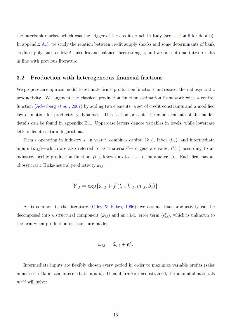
3.2 Production with heterogeneous financial frictions

We propose an empirical model to estimate firms’ production functions and recover their idiosyncratic

productivity. We augment the classical production function estimation framework with a control

function (Ackerberg et al. , 2007) by adding two elements: a set of credit constraints and a modified

law of motion for productivity dynamics. This section presents the main elements of the model;

details can be found in appendix B.1. Uppercase letters denote variables in levels, while lowercase

letters denote natural logarithms.

Firm i operating in industry s, in year t, combines capital (ki,t), labor (li,t), and intermediate

inputs (mi,t)—which are also referred to as “materials”—to generate sales, (Yi,t) according to an

industry-specific production function f(·), known up to a set of parameters βs. Each firm has an

idiosyncratic Hicks-neutral productivity ωi,t:

Yi,t = exp{ωi,t + f (li,t, ki,t,mi,t, βs)}

As is common in the literature (Olley & Pakes, 1996), we assume that productivity can be

decomposed into a structural component (ωi,t) and an i.i.d. error term (εYi,t), which is unknown to

the firm when production decisions are made:

ωi,t = ωi,t + εYi,t

Intermediate inputs are flexibly chosen every period in order to maximize variable profits (sales

minus cost of labor and intermediate inputs). Then, if firm i is unconstrained, the amount of materials

munc will solve:

13

∂ exp{f (li,t, ki,t,munc, β) + ωi,t}

∂m= PM

p,t (4)

where PMp,t is the price of materials faced by firm i, which might depend on its location p.19 In

section 4, we provide evidence that firms acquire less inputs when they receive negative credit supply

shocks. Relying on the first-order condition in (4) would be misleading if firms face heterogeneous

credit constraints. Therefore, we allow for the possibility that intermediate inputs (and other inputs)

face financially generated constraints:

expmi,t ≤ expmmaxi,t =

1

PMp,t

Ki,t−1 · Γ (Bi,t−1, φi,t, ωi,t)

where Bi,t−1 is previous-period debt and Γ is an unknown function. Similar constraints20 are

standard in the literature on financial frictions, such as Moll (2014), Buera & Moll (2015), and

Gopinath et al. (2017), and they can be micro-founded by several market failures. We innovate

by allowing them to depend on firm TFP and credit supply shocks. The results of the paper hold

if we exclude credit rationing and, alternatively, if we assume that firms face heterogeneous costs

of external funds. High-productivity firms might be considered more reliable borrowers and might

therefore be allowed to borrow more, ceteris paribus. We thus assume that Γ is strictly increasing in

its third argument. The quantity of intermediate inputs acquired by firm i is:

mi,t = min{mmaxi,t ,munc

i,t } := m (xi,t, ωi,t, φi,t) (5)

19Gandhi et al. (2011) show that most of the estimation procedures based on the control function approach failto identify the elasticity of output with respect to the flexible inputs (e.g., intermediate inputs). De Loecker &Scott (2016) argue that a researcher can overcome this non-identification result under the assumption that firms faceheterogeneous and autocorrelated input prices. The authors rely on firm-level wages to estimate their model. However,heterogeneity in wages might reflect heterogeneous worker quality or productivity. We, instead, allow local price shocksto affect input real prices and recover all the production function parameters.

20Capital is the only potentially constrained input in most models.

14

where m (·) is unknown and xi,t is a vector containing firm-level inputs (capital, lagged capital,

and labor), prices, and lagged debt. Under standard assumptions, the optimal value of materials is

increasing in productivity ωi,t, equation 5 can therefore be “inverted” (see Olley & Pakes (1996) and

Levinsohn & Petrin (2003)). That is, there exists an (unknown) function h such that:

ωi,t = h (xi,t,mi,t, φi,t)

Therefore, log sales can be written as:

yi,t = Ψ (xi,t,mi,t, φi,t) + εYi,t

where Ψ (xi,t,mi,t, φi,t) = h (xi,t,mi,t, φi,t) + f (li,t, ki,t,mi,t, βs). Following the previous literature,

we assume a law of motion for productivity:

Et [ωi,t|It−1] = Et [ωi,t|ωi,t−1, φi,t−1] = gt (ωi,t−1, φi,t−1) (6)

where It−1 is the firm information set at t−1 and gt (·) is unknown. We innovate by allowing credit

supply to affect productivity dynamics. It would not be correct to estimate the production function

without including financial frictions in the productivity dynamics and regress the productivity resid-

uals on financial variables. An analogous problem is highlighted in De Loecker (2013) discussion of

the measurement of productivity gains from exporting. Let us also define the productivity innovation

as ζi,t := ωi,t − E [ωi,t|It−1]. Equation (6) implies moment conditions:

15

E [ζi,t|It−1] = E [ζi,t|zi,t−1] =

= E

Ψi,t − f (li,t, ki,t,mi,t, β)−

gt (Ψi,t−1 − f (li,t−1, ki,t−1,mi,t−1, β) , φi,t−1)|zi,t−1

= 0(7)

where zi,t−1 contains lagged values of investments, labor, materials, and other variables. Estimation

of the model is performed in two stages. In the first stage, we estimate the function Ψ as Ψi,t =

E [yi,t|xi,t,mi,t, φi,t]. In the second stage, we rely on (7) to estimate the structural parameter of

interest βs. Table A.2 presents some descriptive statistics. Finally, we can back out firm-level

productivity as residuals from ωi,t = yi,t − f (ki,t, li,t,mi,t, βs) or, in the value-added case, ωi,t =

vai,t − f (ki,t, li,t, βs).

As detailed in section 2, we observe balance-sheet and income statements but do not observe

firm-level output prices. Therefore, this paper is about the ability of firms to transform inputs into

sales and value added and not (only) about their technical efficiency. Our measure of productivity is

referred to as “productivity” in several empirical studies, such as Olley & Pakes (1996), and as tfprrr

(or “regression-residual total factor revenue productivity”) in Foster et al. (2017). Furthermore, our

measure of productivity is proportional to the empirical estimate of (log) TFPQ (or “total factor

quantity productivity”) in Hsieh & Klenow (2009). Our choice in this regard is somewhat constrained,

as no firm-level data on product-level prices are available to economists for a sufficiently large number

of Italian firms. Appendix C.1 provides a more detailed treatment of the topic and contains a brief

discussion of the pros and cons of relying on revenues to estimate TFP.

4 Credit Supply Shocks and Firm Production

Is a firm’s production affected by the credit supply of its lenders? If credit frictions are not important,

the amount of credit a firm receives should be unaffected by the supply shocks of its lenders. In a

frictionless world, a firm’s policy function might be affected by aggregate financial conditions but

should not be shaped by the idiosyncratic shocks hitting any specific lender. Therefore, we estimate:

∆xi,t = ψi + ψp,s,t + γ · φi,t + ηi,t (8)

16

where xi,t is either the log of total credit granted to firm i or a measure of output (log value

added or net revenues) produced by firm i during year t or a measure of (log) input. The ψ terms

are firm and year×industry×province fixed effects. The former control for firm-specific unobserved

heterogeneity which might affect both financial conditions and production. The latter capture local21

and sectoral demand and technology shocks, which might create spurious correlation between credit

supply and firm dynamics. Results are presented in Table 2. Firms connected with banks expanding

their supply of credit show higher growth of credit received, inputs acquired, and output produced

than to other firms operating in the same market. The elasticity of credit granted with respect to

the firm-level credit supply shock is approximately equal to 1. This allows for simple interpretation

of the magnitude of all the main specification of this paper: a one-percentage-point increase in φi,t

is the change of credit supply necessary to increase the average credit granted one percent.

The effect of an expansion of credit supply is stronger for value added than for capital accumula-

tion. Net revenues respond almost as much as capital. Labor and intermediate inputs are found to

be much less sensitive to credit supply shocks than output and capital are, from both the economic

and the statistical point of view. Capital investments are likely to be fully paid up front, while

expenditure for materials or labor can sometimes be delayed until some cash flow has been generated

from the production. For instance, wages are usually paid at the end of the month. Therefore, it

is not surprising that these inputs are less sensitive to changes in a firm’s ability to access external

finance. To understand whether the effect on inputs is sufficiently large to rationalize the impact on

output or, conversely, whether productivity is responding to credit shocks, we need to rely on the

elasticities of output to inputs estimated in section 3.2.

5 The Effect of Credit Supply on Firm Productivity Growth

Is firm productivity growth affected by the credit supply of its lenders? After identifying firm-level

measures of credit supply shocks (section 3.1) and measuring TFP (section 3.2), we now tackle the

main research question by estimating the model:21A province is a local administrative unit, approximately of the size of a US county. CADS reports the province in

which each firm is headquartered.

17

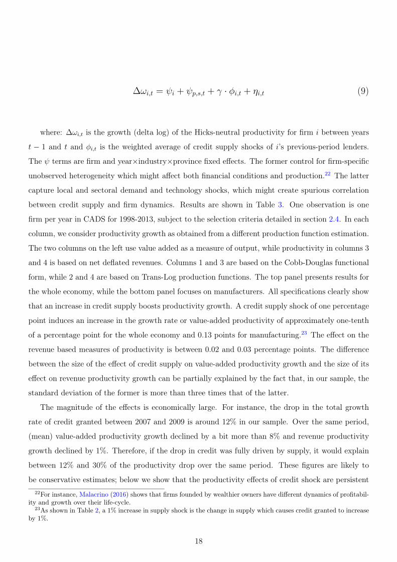
∆ωi,t = ψi + ψp,s,t + γ · φi,t + ηi,t (9)

where: ∆ωi,t is the growth (delta log) of the Hicks-neutral productivity for firm i between years

t − 1 and t and φi,t is the weighted average of credit supply shocks of i’s previous-period lenders.

The ψ terms are firm and year×industry×province fixed effects. The former control for firm-specific

unobserved heterogeneity which might affect both financial conditions and production.22 The latter

capture local and sectoral demand and technology shocks, which might create spurious correlation

between credit supply and firm dynamics. Results are shown in Table 3. One observation is one

firm per year in CADS for 1998-2013, subject to the selection criteria detailed in section 2.4. In each

column, we consider productivity growth as obtained from a different production function estimation.

The two columns on the left use value added as a measure of output, while productivity in columns 3

and 4 is based on net deflated revenues. Columns 1 and 3 are based on the Cobb-Douglas functional

form, while 2 and 4 are based on Trans-Log production functions. The top panel presents results for

the whole economy, while the bottom panel focuses on manufacturers. All specifications clearly show

that an increase in credit supply boosts productivity growth. A credit supply shock of one percentage

point induces an increase in the growth rate or value-added productivity of approximately one-tenth

of a percentage point for the whole economy and 0.13 points for manufacturing.23 The effect on the

revenue based measures of productivity is between 0.02 and 0.03 percentage points. The difference

between the size of the effect of credit supply on value-added productivity growth and the size of its

effect on revenue productivity growth can be partially explained by the fact that, in our sample, the

standard deviation of the former is more than three times that of the latter.

The magnitude of the effects is economically large. For instance, the drop in the total growth

rate of credit granted between 2007 and 2009 is around 12% in our sample. Over the same period,

(mean) value-added productivity growth declined by a bit more than 8% and revenue productivity

growth declined by 1%. Therefore, if the drop in credit was fully driven by supply, it would explain

between 12% and 30% of the productivity drop over the same period. These figures are likely to

be conservative estimates; below we show that the productivity effects of credit shock are persistent22For instance, Malacrino (2016) shows that firms founded by wealthier owners have different dynamics of profitabil-

ity and growth over their life-cycle.23As shown in Table 2, a 1% increase in supply shock is the change in supply which causes credit granted to increase

by 1%.

18

and that credit supply is particularly valuable during financial turmoil.

Appendix figure A.8 reports the bootstrapped distribution of the estimated effect of credit supply

shock on productivity. The production functions are re-estimated for each bootstrap sample. All

coefficients are above zero. This finding indicates that the sampling error in estimating productivity

dynamics does not distort statistical inferences based on Table 3.

5.1 Robustness

This paper argues for a causal interpretation of the estimated relations between credit supply and

firm productivity growth. We provide a broad set of robustness exercises to support this claim. Table

4 contains the relative results for the Cobb-Douglas revenue productivity case.24 Column (1) reports

the baseline estimate (as in Table 3). Column (2) adds a set of lagged controls: a polynomial in

assets size and the ratios of value added, cash flow, liquidity, and bank debt to assets. The inclusion

of such controls has negligible impact on the estimated coefficients.

Estimates of equation (9) face both identification-related threats and measurement threats. This

section deals with the latter and with potential problems related to the estimation of the productivity

dynamics. Measurement error issues are discussed in appendix C.3. Analogously to the “peer effect”

literature (Bramoullé et al. , 2009), three main threats may hamper our identification strategy of

credit supply shocks based on firm-bank connections: reverse causality, correlated unobservables,

and assortative matching. That is, φi,t can be correlated with the error term in equation (9) because

(a) connected agents are subject to correlated shocks, (b) lenders might decrease credit supply when

expecting their borrowers to experience lower productivity growth, or (c) banks which are expanding

their supply of credit are more likely to establish lending relations with firms that are increasing

their productivity.25 The productivity shocks received by sizable borrowers might be the very reason

why their lenders contract the supply of credit. That is, if banks have information about the future

profitability of some particularly significant borrowers, they might preemptively decrease the supply

of credit to all borrowers. We define an “important” borrower as any firm which, at any point

between 1997 and 2013, accounts for more than 1% of the credit granted by any of its lenders. We

then estimate model (9) excluding such firms. Results are reported in column (3) of Table 4, which

shows that the estimated effect of credit supply shocks on productivity growth is unaffected by the24Results for value-added productivity and revenue translog productivity are in Tables A.11 and A.12. They all

show remarkable stability across specifications.25For instance, Bonaccorsi di Patti & Kashyap (2017) document that the banks which recover earlier from distress

are the ones which were quicker to cut their credit to risky borrowers. Notice that the additive growth rate modelallows for assortative matching in levels.

19

exclusion of the borrowers that are most likely to lead to reverse causality, thus mitigating this

concern.

A further concern is that connected borrowers and lenders might be affected by correlated un-

observable shocks. In particular, the output market of the borrower might overlap with the lender’s

collection or lending market. For instance, a drop in local house prices might contemporaneously

lower consumption and also affect the value of collateral backing lenders’ loans. Since we measure

revenue-based productivity, any demand shock might increase markups and be picked up as a change

in productivity. To investigate the relevance of correlated unobservables for our results, we compare

specifications with two different fixed-effects structures:

∆ωi,t = ψi + ψp,s,t + γ · φi,t + ηi,t

∆ωi,t = ψi + ψp + ψs + ψt + γ · φi,t + ηi,t

The first specification includes industry×province×year fixed effects, which aim to control for

demand and technology shocks. The second includes only includes only industry, province, and year

fixed effects; it therefore allows only for nationwide economic fluctuations. Results are reported

in columns (1) and (5) of Table 4. The magnitude of the coefficient is remarkably stable across

the two specifications, despite the fact that the inclusion of the finer grid of fixed effects doubles

the R2. This finding reveals that, if any unobservable is affecting both credit supply shocks and

productivity, then it must be orthogonal with respect to location or industry. Since credit activity

is indeed concentrated at the local (and/or industry) level, this is extremely unlikely to happen.

Consequently, we can reasonably conclude that correlated unobservables are not driving our results.

A formal econometric treatment of this intuitive argument is provided by Altonji et al. (2005) and

Oster (2016). In appendix C.2, we provide bounding sets for the coefficient of interest, following

Oster (2016), and show that they do not contain zero. Therefore, our results are “robust” to the

presence of unobservable shocks. Furthermore, column (4) of Table 4 shows that firm fixed effects,

while useful to control for firm-level unobservable characteristics, are not essential to our results.

Column (6) of Table 4 adopts an alternative measure of credit supply shocks, which controls for

match-level characteristics26 (see appendix A.1 for details). The estimated effect of credit supply on26Namely, the size of the loan relative to the borrower’s total credit received, size of the loan relative to the lender’s

20

productivity growth is similar to that in the baseline specification of column (1), providing no evidence

that assortative matching explains our results. Finally, section 6 exploits a natural experiment to

confirm that credit supply affects productivity; this, together with relative placebo tests, should

eliminate residual concerns.

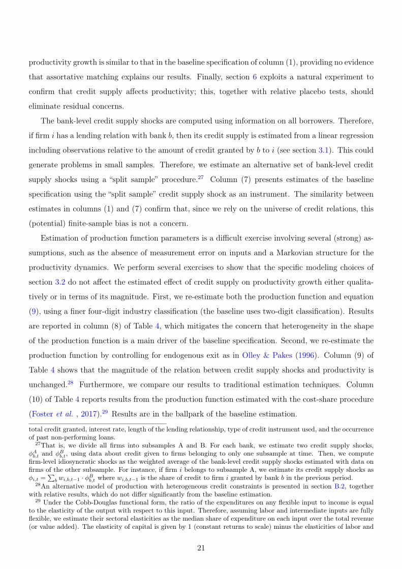
The bank-level credit supply shocks are computed using information on all borrowers. Therefore,

if firm i has a lending relation with bank b, then its credit supply is estimated from a linear regression

including observations relative to the amount of credit granted by b to i (see section 3.1). This could

generate problems in small samples. Therefore, we estimate an alternative set of bank-level credit

supply shocks using a “split sample” procedure.27 Column (7) presents estimates of the baseline

specification using the “split sample” credit supply shock as an instrument. The similarity between

estimates in columns (1) and (7) confirm that, since we rely on the universe of credit relations, this

(potential) finite-sample bias is not a concern.

Estimation of production function parameters is a difficult exercise involving several (strong) as-

sumptions, such as the absence of measurement error on inputs and a Markovian structure for the

productivity dynamics. We perform several exercises to show that the specific modeling choices of

section 3.2 do not affect the estimated effect of credit supply on productivity growth either qualita-

tively or in terms of its magnitude. First, we re-estimate both the production function and equation

(9), using a finer four-digit industry classification (the baseline uses two-digit classification). Results

are reported in column (8) of Table 4, which mitigates the concern that heterogeneity in the shape

of the production function is a main driver of the baseline specification. Second, we re-estimate the

production function by controlling for endogenous exit as in Olley & Pakes (1996). Column (9) of

Table 4 shows that the magnitude of the relation between credit supply shocks and productivity is

unchanged.28 Furthermore, we compare our results to traditional estimation techniques. Column

(10) of Table 4 reports results from the production function estimated with the cost-share procedure

(Foster et al. , 2017).29 Results are in the ballpark of the baseline estimation.

total credit granted, interest rate, length of the lending relationship, type of credit instrument used, and the occurrenceof past non-performing loans.

27That is, we divide all firms into subsamples A and B. For each bank, we estimate two credit supply shocks,φAb,t and φBb,t, using data about credit given to firms belonging to only one subsample at time. Then, we computefirm-level idiosyncratic shocks as the weighted average of the bank-level credit supply shocks estimated with data onfirms of the other subsample. For instance, if firm i belongs to subsample A, we estimate its credit supply shocks asφi,t =

∑b wi,b,t−1 · φBb,t where wi,b,t−1 is the share of credit to firm i granted by bank b in the previous period.

28An alternative model of production with heterogeneous credit constraints is presented in section B.2, togetherwith relative results, which do not differ significantly from the baseline estimation.

29 Under the Cobb-Douglas functional form, the ratio of the expenditures on any flexible input to income is equalto the elasticity of the output with respect to this input. Therefore, assuming labor and intermediate inputs are fullyflexible, we estimate their sectoral elasticities as the median share of expenditure on each input over the total revenue(or value added). The elasticity of capital is given by 1 (constant returns to scale) minus the elasticities of labor and

21

An alternative approach is to refrain from estimating the production function and, instead, study

how the estimated effect of credit supply shocks on productivity varies as a function of the unknown

parameters of the production function. The simplest production function is a Cobb-Douglas in value

added:

vai,t = ωi,t + ρ · (βk · ki,t + (1− βk) · li,t)

where ρ disciplines the returns to scale and βk is the (relative) elasticity of value added to capital.

Then, given a pair (ρ, βk), we can back out productivity as

ωi,t(ρ, βk) = vai,t − ρ ·(βk · ki,t +

(1− βk

)· li,t)

and estimate γ(ρ, βk) as the coefficient of

∆ωi,t(ρ, βk) = ψi + ψp,s,t + γ(ρ, βk) · φi,t + ηi,t (10)

We let ρ vary from 0.3 to 2 and βk from 0.01 to 0.9, so that our grid encompasses any plausible

values of the return to scale and the elasticity of value added to capital. Results are presented in

graphical form in figure 5, showing that we find a positive (and statistically significant) effect of

credit supply shocks on value-added productivity growth for any point on the grid. Moreover, while

higher values of the parameters tend to decrease the point estimates, γ(ρ, βk) stays between 0.07 and

0.1 within the whole support.

The collection of evidence reported in this section clarifies that any misspecification of the pro-

intermediates. Foster et al. (2017) describe the theoretical and empirical differences between the cost-share approachand the control function. We divide intermediate inputs into expenditure for services and expenditure for materialsin order to show that merging them together does not drive the baseline results of the paper. Doing so, we lose someobservations, since not all income statements report expenditure on the two items separately.

22

duction function estimation, although it might bias the point-estimate of the effect of credit supply

on productivity, is unlikely to change its magnitude significantly.

5.2 Heterogeneity

Are all firms equally affected by credit supply shocks? A firm’s size might be a good predictor of

its ability to find alternative sources of credit in case current lenders dry up. Furthermore, larger

firms are less likely to be credit-constrained in the first place. Therefore, for each year, we compute

an indicator for whether or not a firm is in the top quartile of the size distribution in terms of asset

value or number of employees. Then, we estimate the equation:

∆ωi,t = ψi + ψs,p,t + (γ + γbig ·Bigi,t−1) · φi,t + ψBig ·Bigi,t−1 + ηi,t

Results are reported in columns (1) and (2) of Table 5, which refer to Cobb-Douglas revenue

productivity. The parameter γbig is estimated to be negative, indicating that large firms are less af-

fected by credit supply shocks. The difference between the two groups is much larger and statistically

significant in manufacturing.

Furthermore, we are interested in understanding whether having a larger number of lenders might

help firms find sources of finance in case of negative credit supply shocks. Therefore, we estimate

the model by allowing the coefficient to be different for firms in the bottom quartile for number of

lending relations during the previous period.30 Results in column (3) document that borrowers with

fewer lenders are much more affected by credit supply shocks.

An important dimension of the relevance of credit supply shocks is firms’ reliance on external

funds. We classify industries as above and below the median according to the mean leverage (debt

over assets) in the sample. Column (4) of Table 5 shows that the effect of credit supply shocks on

revenue productivity is stronger in sectors with high leverage. Perhaps surprisingly, we do not find

any significant pattern when analyzing heterogeneity according to sectoral cash flow over assets (see

column (5)).30A few seminar participants suggested differentiating the effect of credit shocks between firms with one and with

multiple lending relationships. Unfortunately, less than 5% of the observations in CADS have only one lender, so therelative coefficient would not be reliably estimated.

23

5.3 Persistence

The effect of credit supply on productivity is persistent. We define the innovation to the credit

supply as ζφi,t := φi,t − E [φi,t|φt−1]. Then, we estimate the model

ωi,t = ψi + ψp,s,t +T∑

τ=−T

γτ · ζφi,t + ηi,t (11)

We choose T = 3, since our empirical strategy is not fit to estimate the regression at a longer

horizon.31 Figure 4 graphically displays the coefficients, γτ , for firms active in manufacturing (bottom

panel) and all industries (top panel). They document that the peak in productivity is experienced one

year after the shock and that the effect remains positive and significant for at least four years. This

finding underlines that a temporary credit contraction can have persistent effects on productivity. It

also rules out the potential concern that the effect we measure on revenue productivity is short-lived

and due to factor hoarding caused by adjustment costs of labor and capital.

We do not find any statistically significant pre-trend. Our main results rely on pre-existing lending

relations being orthogonal with respect to non-financial productivity shocks. Therefore, the absence

of a pre-trend supports the claim that credit supply shocks have a causal effect on productivity.

5.4 Concavity of the credit-productivity relationship

The main goal of this paper is to measure and explain the productivity effects of changes in the

quantity of credit supplied, focusing on its first moment: is more credit bad or good? This section,

instead, investigates the shape of the relation between productivity and credit supply shocks, in order

to understand whether higher moments of the distribution of credit supply shocks might have an

impact on average firm productivity.31 The within-firm estimator, while allowing us to control for firm unobserved heterogeneity, creates a mechanical

negative correlation between observation means at different lags. In fact, regression of firm productivity on pastproductivity yields a coefficient between .9 and .98 if no fixed effects are included and between .3 and .4 if thestandard set of fixed effects is included. Therefore, a shock to productivity of magnitude 1 ·m, is expected to showup as a change in productivity of only 0.03 ·m to 0.06 ·m after 3 years.

24

We divide φi,t into quintiles q = 1, 2, 3, 4, 5 and estimate:

∆ωi,t = ψi + ψp,s,t +5∑

q=1,q 6=3

γq · 1 (φi,t ∈ q) + ηi,t

where 1 (φi,t ∈ q) is an indicator function taking value 1 iff the credit supply shock of firm i in year

t belongs to the qth quintile of its distribution; the third (or median) quintile q = 3 is the omitted

category with γ3 = 0. Results are shown in graphical form in figure 6. The relation between credit

supply and revenue productivity seems to be concave. That is, firms connected with banks with a

relatively low supply of credit experience lower revenue productivity growth than their competitors;

firms connected to banks with a particularly strong increase in credit do not grow at a particularly

high rate. It is important not to be connected with banks experiencing bad credit supply shocks,

but it is not useful to be connected with banks increasing their supply of credit particularly quickly.

To strengthen this intuition, we re-estimate equation (11), which is used to study the persistence of

credit supply shocks, by differentiating between positive and negative shocks. Figure 7 presents the

results in graphical form. The coefficients relative to negative credit supply shocks are shown with

negative values. The effect of credit supply shocks on productivity is driven by firms connected with

banks experiencing relatively negative credit supply dynamics. Additionally, we argue in section 6

that credit supply shocks are particularly important when credit dries up.

These empirical findings imply that an increase in credit supply cannot undo the harm of a

negative shock of the same size. Therefore, it is not only the quantity of credit that matters, but also

the stability of its provision. This analogously suggests that a credit crunch followed (or preceded)

by a credit expansion of the same magnitude leads to a net loss in average firm productivity. We

conclude that the volatility of the banking sector’s supply can be detrimental to firm productivity.

6 The Interbank Market Collapse as a Natural Experiment

The credit supply shock derived in section 3.1 has the value of being general, in that it can be

attributed to all firms (both multiple- and single-borrowers) and measured in any year for which

there is bank-firm data on credit granted. This feature is exploited in section 7. Furthermore, the

panel variation of φi,t is essential for production function estimation (see section 3.2). However,

since its construction relies on firm-bank connections, estimates of equation (9) might suffer from

25

the identification problems highlighted in section 5.1. Although we have already discussed several

robustness exercises to mitigate such concerns, here we propose an alternative strategy to strengthen

the robustness of our results. We use the 2007-2008 market collapse of the interbank market as a

specific “natural experiment” in which credit supply shifts were arguably exogenous with respect to

firm observed and unobserved characteristics.32 In addition, such variation came unexpectedly both

to lenders and to borrowers, thus overcoming the problem of assortative matching.

The interbank market is a critical source of funding for banks: it allows them to readily fill liquidity

needs of different maturities through secured and unsecured contracts. Total gross interbank funding

accounted for over 13% of total assets of Italian banks at the end of 2006. Market transactions began

shrinking in July 2007, when fears about the spread of toxic assets in banks’ balance sheets made

the evaluation of counterparty risk extremely difficult (Brunnermeier, 2009); the situation worsened

further after Lehman’s default in September 2008. As a consequence, total transactions among banks

fell significantly. In Italy, in particular, they plummeted from e24bn. in 2006 to e4.8bn. at the

end of 2009. At the same time, the cost of raising funds in the interbank market rose sharply: the

Euribor-Eurepo spread, which was practically zero until August 2007, reached over 50 basis points

for all maturities in the subsequent year. It then increased by five times after the Lehman crisis and

remained well above 20 basis points in the following years. Two recent papers have exploited the

collapse of the interbank market as a source of exogenous shock to credit supply. Iyer et al. (2013)

used Spanish data to show that bank pre-crisis exposure to the interbank shock, as measured by the

ratio of interbank liabilities to assets, was a significant predictor of a drop in credit granted during the

crisis. Cingano et al. (2016) focus on CADS data for Italy to show that this drop had a significant

negative effect on firms’ capital accumulation. These researchers reported results of several empirical

tests showing that banks’ pre-crisis exposure was not correlated with their borrowers’ characteristics,

such as investment opportunities and firm growth potential, thus making this variable particularly

suitable to instrument the impact of credit supply on firms’ outcomes. We focus on the period 2007-

2009, when credit dried up the most. Subsequently, ECB interventions partially offset the impact

of the interbank market shock. Our measure of firm exposure to the credit supply tightening is the

average 2006 interbank exposure of Italian banks at the firm level, using firms’ specific credit shares

in 2006 as weights. Because firm exposure is time-invariant, we use cross-sectional variation. We

include observations over a three-year window. Formally, for each firm i active in industry s and

province p over the years t ∈ [2007, 2009], we estimate the equation:32This is not the first paper to rely on natural experiments to identify idiosyncratic credit supply shocks; see, for

instance, Khwaja & Mian (2008), Chodorow-Reich (2013), and Paravisini et al. (2014).

26

∆ωi,t = ψp,s,t + γ · INTBKi,2006 + ηi,t (12)

where ωi,t is firm idiosyncratic productivity, INTBKi,2006 is the pre-crisis reliance on the interbank

market, and ψ is a set of province×industry×year fixed effects. Results are shown in Table 6. Firms

whose lenders were more reliant on the interbank market in 2006 had significantly lower revenue and

value-added productivity growth during the credit crunch. This strengthens the causal interpretation

of the relations between credit supply and productivity growth documented in section 5. A 1%

increase in average bank dependence on the interbank market results in an approximately .05%

decrease in average value-added productivity growth and an approximately .02% decrease in revenue

productivity growth. Consequently, the same interbank shock which decreases credit growth by 1%

also decreases value-added productivity of 0.25% and revenue productivity by one-tenth of a percent

for the whole sample. These effects are between two and five times larger than the baseline estimate

from Table 3, suggesting that accessing a reliable source of credit supply is particularly important

during financial turmoil.

6.1 Placebo and robustness tests

Estimation of (12) provides evidence that firms hit harder by the credit crunch decrease their relative

productivity. What if banks relying more heavily on the interbank market were just matched to worst

borrowers? To remove this concern, we run equation (12) including only years before the freeze of the

interbank market; that is, t ∈ [2004, 2006]. Results, shown in columns (1)—(4) of Table 7, show that

firms more exposed to the freeze of the interbank market did not have statistically different growth

rates of productivity before the credit crunch. Additional results show that firms more exposed to

the interbank shock were not more sensitive to business-cycle fluctuation before 2007. Details are

in appendix D. We implement an additional placebo test. That is, we investigate the effect of a

hypothetical freeze of the interbank market in 2003. For t ∈ [2003, 2005] we estimate the model:

∆ωi,t = ψp,s,t + γ · INTBKi,2002 + ηi,t

Columns (5)—(8) of Table 7 show that the placebo collapse is not a significant predictor of firms’

27

subsequent productivity growth.

The collection of evidence presented in this section should eliminate the concern that the relation

between credit supply and productivity documented in section 5 is driven by correlated unobservables,

reverse causality, or assortative matching.

7 Beyond Measurement: Channels

How does credit supply improve productivity? In this section, we investigate the relations between the

credit supply shocks and several productivity-enhancing activities. As described in section 2, INVIND

provides information about R&D investment, export, IT-adoption, and self-reported “obstacles to

innovation” for a sample of Italian companies in services and manufacturing. Because both questions

and respondents vary between waves, each specification of this section relies on a different sample.

Furthermore, the sample size is much smaller than in the previous sections, limiting our ability to

use our preferred specification.

In section 5.3, we show that credit supply shocks affect productivity immediately. We detect

additional productivity growth for at least two years and higher productivity for at least four years.

Unfortunately, our empirical framework is not fit to investigate the effect at a longer horizon. Some

of the productivity-enhancing strategies studied in this section, such as IT-adoption or better man-

agement practices, are likely to affect productivity as soon as they are implemented. Others, such as

R&D, might take a few years to produce substantial improvement. Therefore, this section does not

only explore the potential mechanisms behind the effect we measure in section 5, but also suggests

that credit availability might lead to additional productivity gains in the long run.

7.1 IT-intensity of capital stock

The speed of adoption of IT technologies caused large differences in productivity between US and

European companies (Bloom et al. , 2012). According to Pellegrino & Zingales (2014), failure to

take full advantage of the IT revolution is one of the main drivers of Italy’s low productivity growth.

Data on personal computers used is available from INVIND for 1999-2001. Purchases of PCs are

accounted as investments. Therefore, they enter the computation of capital stock. Slacker credit

constraints might allow firms to stay closer to the technological frontier. By making more technolog-

ical investments, unconstrained firms might have a “better” capital stock. Since researchers do not

have detailed information on “quality” or “closeness to the frontier” of inputs, this quality is picked

28

up by the productivity residual. To test this hypothesis, we measure the “IT-intensity” of firm capital

stock as (log) number of PCs per 1,000 euros of capital.

ITi,t = ψi + ψs,p,t + γ · φi,t + ηi,t

Results are presented in column (1) of Table 8. Firms are more likely to increase the IT-intensity

of their capital stock when they receive a positive credit supply shock. This finding suggests that

financial frictions lower the quality of capital inputs used in production.

7.2 Innovation and exporting

Patenting activities have been extensively used as a proxy for firm-level knowledge creation (see

Bernstein (2015) and Kogan et al. (2017) for recent examples). We obtain information for patent

applications for a large fraction of Italian companies from PatStat, as described in section 2. In

our sample, patent applications became much less common during (and after) the credit crunch.

The share of firms applying for at least one patent was approximately 2% between 2002 and 2007.

It declined to 1.5% in 2009 and went up to a bit more than 1.6% in the following two years. We

observe approximately 5 patent applications per 100 firms per year before the Great Recession, but

only around 3.4 in 2009. This pattern, of course, could be driven by lower demand and/or greater

uncertainty. To investigate whether availability of credit has a causal impact on patent applications,

we estimate the models:

PatentAppi,t = ψi + ψp,s,t + γ · φi,t−1 + ηi,t

GrowthPatentAppi,t = ψi + ψp,s,t + γ · φi,t−1 + ηi,t

Following the literature on R&D and patents, we impose a lag between the credit shock and

patent applications. The growth rate of patent applications is defined as GrowthPatentAppi,t =

29

2PatentAppi,t−PatentAppi,t−2

PatentAppi,t+PatentAppi,t−2.33 Results are reported in columns (2) and (3) of Table 8. Italian firms

patent more when they have easier access to bank credit. Appendix D.3 uses the collapse of the

interbank market to provide additional evidence on the causal effect of the tightening of credit

constraints on innovation.

R&D can increase firm productivity by improving both product quality and process efficiency.

Similarly, export can have beneficial effects through two channels: it allows firms to access markets

with higher margins and it can improve firm know-how through so called “learning-by-exporting.” The

sensitivity of international trade to financial frictions has been studied by several authors (Manova,

2012). We use the INVIND survey to identify firms that export and that have positive R&D expen-

ditures. We focus on the extensive margin and estimate two linear probability models:

Pr(R&Di,t = 1) = ψi + ψt + γ · φi,t + ηi,t

Pr(Exporti,t = 1) = ψi + ψt + γ · φi,t + ηi,t

where R&Di,t and Exporti,t are dummy variables indicating whether firm i engages in R&D or

exporting in year t. Results, presented in columns (4) and (5) of Table 8, show that there is a

positive and statistically significant relation between credit supply and the propensity for these

productivity-enhancing activities. This indicates that companies are more likely to start (and less

likely to stop) conducting R&D and exporting when they have easier access to external finance.

Innovative effort is much broader than just formal R&D or IT-adoption. The 2011 survey wave

investigates the main constraints to innovative effort. One question asks how important, on a four-

item scale, the firm’s difficulties in collecting external funds were in limiting innovation (in 2010).

We build the variable FinConi,2010, equal to 1 if and only if difficulty in getting external funds is

reported to be “somehow important” or “very important” as an obstacle to innovation. Then, we

estimate the linear probability model:

Pr(FinConi,2010 = 1) = ψs,p + γ · φi,2010 + ηi33 In the rest of the paper, we measures growth rates of credit, inputs, output, and TFP using a delta-log approx-

imation. However, patent applications are rare, so we rely on the well-known formula by Davis et al. (1996), whichcan be calculated if patent applications are positive either in year t or t−2 (or both). We use a two-periods lag ratherthan one because we have a lagged right-hand-side variable.

30

Results are presented in column (6) of Table 8, which documents that firms receiving positive

credit supply shocks are less likely to consider external funds as a substantial obstacle to innova-

tion. Since the question was asked for only one year of the survey, we cannot use panel variation.

Nonetheless, this exercise is an indirect—yet insightful—test of the hypothesis that financial frictions

dampen firms’ innovative efforts.

7.3 Management practices

Management matters for firm performance, as shown by Bloom et al. (2013) for India and by Giorcelli

(2016) for Italy. We use credit supply shocks to investigate whether firms improve their management

when facing slacker financial constraints. The direction of the relation is not obvious. Scarcity

of resources might push firms to improve their internal organization. Conversely, improvement in

management practices might require stable financial resources; for instance, to hire professional

consulting services or to restructure a production facility. Bhattacharya et al. (2013) propose a

model in which frictions distort optimal investment in managerial skills.

We obtain firm-level data on management practices from theWorld Management Survey (WMS).34

As can be read from the website, WMS “developed an in-depth survey methodology and constructed

a robust measure of management practices in order to investigate and explain differences in man-

agement practices across firms and countries in different sectors.” Information on data construction

can be found in Bloom & Van Reenen (2007). They state that the “practice evaluation tool defines

and scores from one (worst practice) to five (best practice) across eighteen key management practices

used by industrial firm.” Merging WMS data on Italian companies by name, we obtain a sample

of 183 observations. Because we have only one or two survey waves for each firm, we estimate the

cross-sectional model:

MSi,t = ψ + γ · φi,t + ηi,t

where MSi,t is the overall management score for firm i surveyed in year t. Results are presented

in column (7) of Table 8, which indicates that an increase in credit supply stimulates the adoption34 See http://worldmanagementsurvey.org/. We are grateful for the data provided.

31

of superior management practices. While the small sample size might cast doubt on the robustness

of this result, the relation between credit supply shock and management is largely unaffected by the

inclusion of a large set of firm-level controls.

7.4 Managerial inattention

We propose a novel theory to explain why firms subject to negative credit shocks might decrease

their productivity. Dealing with investors and creditors takes a substantial share of executive time.

Bandiera et al. (2011) study the use of time by 94 CEOs of top-600 Italian companies. They

document that finance is the topic on which the CEO spends the most time talking with others

in the firm. Furthermore, of the outsiders with whom CEOs spend the most time, investors and

bankers are, respectively, third and fifth. If this is true for Italian top-600 companies, which are all

likely to have a professional CFO and other finance-related personnel, the time and effort required to

establish and maintain relations with lenders might be even more demanding for the managers and

entrepreneurs of smaller private companies which make up the bulk of our sample. Since their time

is limited (as in a “temporal” limited span of control35), then the more difficult (or time-consuming)

it is to find external funds, the less they can work on improving their core business. Entrepreneurs

connected to lenders who contract their credit supply might need to spend more time and energy

to establish new lending relations. Therefore, they might exert less effort in improving their firm’s

productivity. As a colorful piece of anecdotal evidence to support this theory, the aunt of one of the

authors was managing the family business during the credit crunch. When asked about the firm’s

performance, she used to reply, “I barely have time to go to the factory, I spend most of my mornings

at banks trying to get some money.” As an indirect test of this mechanism, appendix A.2 and the

relative results in Table A.1 show that firms receiving positive credit supply shocks are less likely to

try to establish new lending relations. A more direct and complete investigation of this hypothesis

is left to future research.

8 Conclusion

To grow and thrive, firms need reliable access to external funding. In particular, this paper carefully

documents that credit supply is an important determinant of improving a firm’s performance, both

in the short run and in the long run.35See Akcigit et al. (2016) for an example of the harm caused by the lack of managerial delegation in developing

countries.

32

We therefore study the impact of banks’ credit supply on production for a large sample of Italian

corporations. We exploit the universe of bank-firm credit relationship over the period 1997-2013 to

estimate an additive growth rate model and we separate demand from supply shocks using firm-time

and bank-time fixed effects. We improve on the literature by considering two important extensions

to this framework. Then, we use the estimated bank-level supply shocks and the stickiness of lending

relationship to build a measure of firm-specific shocks to credit supply. We document that firms

connected to banks which are expanding their supply of credit acquire more inputs and produce

more outputs than their competitors. We show that the effect on output is stronger than the effect

on inputs, suggesting that productivity is affected by credit availability.

We build a model of production with heterogeneous credit constraints in order to estimate an

industry-specific production function and isolate firm idiosyncratic productivity dynamics. Then, we

show that credit supply boosts productivity growth and that these effects are sizable, persistent, and

robust. Moreover, they are stronger for smaller firms and for companies in sectors relying heavily on

banking credit. Furthermore, we exploit the 2007-2008 freeze of the interbank market as a natural

experiment to support the causal interpretation of our estimates and show that they are not driven

by the assortative matching of borrowers and lenders or by reverse causality. Our results imply that

financial turmoil can have a persistent effect on aggregate output because it depresses firms’ TFP in

the short and long run. Furthermore, our findings suggest that financial frictions are harmful beyond

their detrimental effects on allocative efficiency.

We show that a negative credit supply shock produces stronger effects than a positive one of the

same magnitude. This finding implies that it is not only the quantity of credit supply that matters,

but also its stability.

Finally, we show that several productivity-enhancing activities, such as IT-adoption, sound man-

agement practices, export, and innovation, are stimulated by credit availability. We also conjecture

that a reduction of credit supply might force borrowers’ managers/entrepreneurs to consume time

and energy in order to establish connections with additional lenders. Consequently, they might exert

less effort in improving business performance. We document that firms’ attempts to create new

lending relationships are indeed more frequent when experiencing negative credit shocks.

ReferencesAckerberg, Daniel, Benkard, C Lanier, Berry, Steven, & Pakes, Ariel. 2007. Econometric tools for analyzing market

outcomes. Handbook of econometrics, 6, 4171–4276.

Ackerberg, Daniel A., Caves, Kevin, & Frazer, Garth. 2015. Identification Properties of Recent Production FunctionEstimators. Econometrica, 83(6), 2411–2451.

33

Adler, Gustavo, Duval, Mr Romain A, Furceri, Davide, Sinem, K, Koloskova, Ksenia, Poplawski-Ribeiro, Marcos,et al. . 2017. Gone with the Headwinds: Global Productivity. International Monetary Fund.

Aghion, Philippe, Angeletos, George-Marios, Banerjee, Abhijit, & Manova, Kalina. 2010. Volatility and growth: Creditconstraints and the composition of investment. Journal of Monetary Economics, 57(3), 246–265.

Aghion, Philippe, Askenazy, Philippe, Berman, Nicolas, Cette, Gilbert, & Eymard, Laurent. 2012. Credit constraintsand the cyclicality of R&D investment: Evidence from France. Journal of the European Economic Association,10(5), 1001–1024.

Akcigit, Ufuk, Alp, Harun, & Peters, Michael. 2016. Lack of selection and limits to delegation: firm dynamics indeveloping countries. NBER working paper.

Altonji, Joseph G, Elder, Todd E, & Taber, Christopher R. 2005. Selection on observed and unobserved variables:Assessing the effectiveness of Catholic schools. Journal of political economy, 113(1), 151–184.

Amiti, Mary, & Weinstein, David E. 2017. How much do idiosyncratic bank shocks affect investment? Evidence frommatched bank-firm data. Journal of Political Economy.

Anzoategui, Diego, Comin, Diego, Gertler, Mark, & Martinez, Joseba. 2016. Endogenous Technology Adoption andR&D as Sources of Business Cycle Persistence. NBER working paper.

Asker, John, Collard-Wexler, Allan, & De Loecker, Jan. 2014. Dynamic inputs and resource (mis) allocation. Journalof Political Economy, 122(5), 1013–1063.

Bandiera, Oriana, Guiso, Luigi, Prat, Andrea, & Sadun, Raffaella. 2011. What do CEOs do?

Bartelsman, Eric, Haltiwanger, John, & Scarpetta, Stefano. 2013. Cross-country differences in productivity: The roleof allocation and selection. The American Economic Review, 103(1), 305–334.

Begenau, Juliane, Piazzesi, Monika, & Schneider, Martin. 2015. Banks’ risk exposures. NBER working paper.

Benfratello, Luigi, Schiantarelli, Fabio, & Sembenelli, Alessandro. 2008. Banks and innovation: Microeconometricevidence on Italian firms. Journal of Financial Economics, 90(2), 197–217.

Bentolila, Samuel, Jansen, Marcel, Jiménez, Gabriel, & Ruano, Sonia. 2013. When credit dries up: Job losses in thegreat recession.

Bernstein, Shai. 2015. Does going public affect innovation? The Journal of Finance, 70(4), 1365–1403.

Besley, Timothy, Roland, Isabelle, & Van Reenen, John. 2017. Credit Market Frictions and the Productivity Slowdown.mimeo.

Bhattacharya, Dhritiman, Guner, Nezih, & Ventura, Gustavo. 2013. Distortions, endogenous managerial skills andproductivity differences. Review of Economic Dynamics, 16(1), 11–25.

Bloom, Nicholas, & Van Reenen, John. 2007. Measuring and Explaining Management Practices Across Firms andCountries*. The Quarterly Journal of Economics, 122(4), 1351–1408.

Bloom, Nicholas, Sadun, Raffaella, & Van Reenen, John. 2012. Americans do IT better: US multinationals and theproductivity miracle. The American Economic Review, 102(1), 167–201.

Bloom, Nicholas, Eifert, Benn, Mahajan, Aprajit, McKenzie, David, & Roberts, John. 2013. Does managementmatter? Evidence from India. The Quarterly Journal of Economics, 128(1), 1–51.

Bloom, Nicholas, Jones, Charles, Van Reenen, John, & Webb, Michael. 2016. Are ideas getting harder to find?Unpublished paper, Stanford University.

Bonaccorsi di Patti, Emilia, & Kashyap, Anil. 2017. Which Banks Recover From Large Adverse Shocks? NBERworking paper.

34

Bond, Stephen, Harhoff, Dietmar, Van Reenen, John, et al. . 2005. Investment, R&D and financial constraints inBritain and Germany. Annales d’Économie et de Statistique.

Borio, Claudio EV, Kharroubi, Enisse, Upper, Christian, & Zampolli, Fabrizio. 2016. Labour reallocation and pro-ductivity dynamics: financial causes, real consequences. BIS working paper.

Bottero, Margherita, Lenzu, Simone, & Mezzanotti, Filippo. 2015. Sovereign debt exposure and the bank lendingchannel: impact on credit supply and the real economy.

Bramoullé, Yann, Djebbari, Habiba, & Fortin, Bernard. 2009. Identification of peer effects through social networks.Journal of econometrics, 150(1), 41–55.

Broner, Fernando, Erce, Aitor, Martin, Alberto, & Ventura, Jaume. 2014. Sovereign debt markets in turbulent times:Creditor discrimination and crowding-out effects. Journal of Monetary Economics, 61, 114–142.

Brunnermeier, Markus K. 2009. Deciphering the liquidity and credit crunch 2007–2008. The Journal of economicperspectives, 23(1), 77–100.

Brunnermeier, Markus K, Eisenbach, Thomas M, & Sannikov, Yuliy. 2012. Macroeconomics with financial frictions:A survey. NBER working paper.

Buera, Francisco J, & Moll, Benjamin. 2015. Aggregate implications of a credit crunch: The importance of hetero-geneity. American Economic Journal: Macroeconomics, 7(3), 1–42.

Buono, Ines, & Formai, Sara. 2013. Bank Credit and Firm Export: Is there really a link? FREIT Working Paper.

Butler, Alexander W, & Cornaggia, Jess. 2011. Does access to external finance improve productivity? Evidence froma natural experiment. Journal of Financial Economics, 99(1), 184–203.

Byrne, David M, Fernald, John G, & Reinsdorf, Marshall B. 2016. Does the United States have a productivityslowdown or a measurement problem? Brookings Papers on Economic Activity, 2016(1), 109–182.

Caggese, Andrea. 2016. Financing constraints, radical versus incremental innovation, and aggregate productivity. Tech.rept.

Calligaris, S, Del Gatto, M, Hassan, F, Ottaviano, GIP, Schivardi, F, et al. . 2016. Italy’s productivity conundrum.a study on resource misallocation in Italy. Tech. rept. Directorate General Economic and Financial Affairs (DGECFIN), European Commission.

Carroll, Christopher Dixon. 2001. Death to the log-linearized consumption Euler equation!(And very poor health tothe second-order approximation). Advances in Macroeconomics, 1(1).

Cerra, Valerie, & Saxena, Sweta Chaman. 2008. Growth Dynamics: The Myth of Economic Recovery. AmericanEconomic Review, 98(1), 439–57.

Cette, Gilbert, Fernald, John, & Mojon, Benoit. 2016. The pre-Great Recession slowdown in productivity. EuropeanEconomic Review, 88, 3–20.

Chaney, Thomas, Huang, Zongbo, Sraer, David Alexandre, & Thesmar, David. 2015. Aggregate Effects of CollateralConstraints. mimeo.

Chevalier, Judith A, & Scharfstein, David S. 1996. Capital-Market Imperfections and Countercyclical Markups:Theory and Evidence. The American Economic Review, 703–725.

Chodorow-Reich, Gabriel. 2013. The employment effects of credit market disruptions: Firm-level evidence from the2008–9 financial crisis. The Quarterly Journal of Economics, 129(1), 1–59.

Cingano, Federico, Manaresi, Francesco, & Sette, Enrico. 2016. Does credit crunch investment down? New evidenceon the real effects of the bank-lending channel. The Review of Financial Studies, 29(10), 2737–2773.

Collard-Wexler, Allan, & De Loecker, Jan. 2016. Production function estimation with measurement error in inputs.Tech. rept. National Bureau of Economic Research.

35

Davis, Steven J, & Haltiwanger, John. 2014. Labor market fluidity and economic performance. NBER working paper.

Davis, Steven J, Haltiwanger, John, & Schuh, Scott. 1996. Small business and job creation: Dissecting the myth andreassessing the facts. Small business economics, 8(4), 297–315.

De Loecker, Jan. 2011. Product differentiation, multiproduct firms, and estimating the impact of trade liberalizationon productivity. Econometrica, 79(5), 1407–1451.

De Loecker, Jan. 2013. Detecting learning by exporting. American Economic Journal: Microeconomics, 5(3), 1–21.

De Loecker, Jan, & Scott, Paul T. 2016. Estimating market power Evidence from the US Brewing Industry. Tech.rept. National Bureau of Economic Research.

De Loecker, Jan, & Warzynski, Frederic. 2012. Markups and firm-level export status. The American Economic Review,102(6), 2437–2471.

de Ridder, Maarten. 2016. Investment in Productivity and the Long-Run Effect of Financial Crisis on Output.

Decker, Ryan, Haltiwanger, John, Jarmin, Ron, & Miranda, Javier. 2014. The Role of Entrepreneurship in US JobCreation and Economic Dynamism. The Journal of Economic Perspectives, 28(3), 3–24.

Di Nola, Alessandro. 2015. Capital Misallocation during the Great Recession. Working Paper.

Dörr, Sebastian, Raissi, Mr Mehdi, & Weber, Anke. 2017. Credit-Supply Shocks and Firm Productivity in Italy.

Duval, Romain, Hong, Gee Hee, Timmer, Yannick, et al. . 2017. Financial Frictions and the Great ProductivitySlowdown. Tech. rept. International Monetary Fund.

Fazzari, Steven M, Hubbard, R Glenn, Petersen, Bruce C, Blinder, Alan S, & Poterba, James M. 1988. Financingconstraints and corporate investment. Brookings papers on economic activity, 1988(1), 141–206.

Feldstein, Martin. 2015. The US underestimates growth. Wall Street Journal, 18.

Fernald, JOHN G, Hall, Robert E, Stock, James H, & Watson, Mark W. 2017. The Disappointing Recovery of Outputafter 2009. Brookings Papers on Economic Activity.

Ferrando, Annalisa, & Ruggieri, Alessandro. 2015. Financial constraints and productivity: evidence from euro areacompanies.

Field, Alexander J. 2003. The Most Technologically Progressive Decade of the Century. The American EconomicReview, 93(4), 1399–1413.

Foster, Lucia S, Grim, Cheryl A, Haltiwanger, John, Wolf, Zoltan, et al. . 2017. Macro and Micro Dynamics ofProductivity: From Devilish Details to Insights. NBER working paper.

Gamberoni, Elisa, Giordano, Claire, & Lopez-Garcia, Paloma. 2016. Capital and labour (mis) allocation in the euroarea: some stylized facts and determinants.

Gandhi, Amit, Navarro, Salvador, & Rivers, David A. 2011. On the identification of production functions: Howheterogeneous is productivity?

Garcia-Macia, Daniel. 2015. The financing of ideas and the great deviation. IMF working paper.

Gatti, Roberta, & Love, Inessa. 2008. Does access to credit improve productivity? Evidence from Bulgaria. Economicsof Transition, 16(3), 445–465.

Giorcelli, Michela. 2016. The Long-Term Effects of Management and Technology Transfers.

Gopinath, Gita, Kalemli-Özcan, Şebnem, Karabarbounis, Loukas, & Villegas-Sanchez, Carolina. 2017. Capital alloca-tion and productivity in South Europe. The Quarterly Journal of Economics, qjx024.

Gordon, Robert J. 2016. The rise and fall of American growth: The US standard of living since the civil war. PrincetonUniversity Press.

36

Gordon, Robert J, et al. . 2015. Secular Stagnation on the Supply Side: US Producivity Growth in the Long Run.Communications & Strategies, 1(100), 19–45.

Gorton, Gary, & Ordoñez, Guillermo. 2016. Good booms, bad booms. NBER working paper.

Greenstone, Michael, Mas, Alexandre, & Nguyen, Hoai-Luu. 2014. Do credit market shocks affect the real economy?Quasi-experimental evidence from the Great Recession and ‘normal’economic times. NBER working paper.

Hall, Bronwyn H. 2011. Innovation and productivity. NBER working paper.

Hall, Bronwyn H, & Lerner, Josh. 2010. The financing of R&D and innovation. Handbook of the Economics ofInnovation, 1, 609–639.

Hall, Bronwyn H, Lotti, Francesca, & Mairesse, Jacques. 2008. Employment, innovation, and productivity: evidencefrom Italian microdata. Industrial and Corporate Change, 17(4), 813–839.

Hassan, Fadi, di Mauro, Filippo, & Ottaviano, Gianmarco IP. 2017. Banks credit and productivity growth. Workingpaper.

Hottman, Colin J, Redding, Stephen J, & Weinstein, David E. 2016. Quantifying the sources of firm heterogeneity.The Quarterly Journal of Economics, 131(3), 1291–1364.

Hsieh, Chang-Tai, & Klenow, Peter J. 2009. Misallocation and manufacturing TFP in China and India. The Quarterlyjournal of economics, 124(4), 1403–1448.

Huber, Kilian. 2017. Disentangling the Effects of a Banking Crisis: Evidence from German Firms and Counties.mimeo.

Iyer, Rajkamal, Peydró, José-Luis, da Rocha-Lopes, Samuel, & Schoar, Antoinette. 2013. Interbank liquidity crunchand the firm credit crunch: Evidence from the 2007–2009 crisis. The Review of Financial Studies, 27(1), 347–372.

Jensen, Michael C. 1986. Agency costs of free cash flow, corporate finance, and takeovers. The American economicreview, 76(2), 323–329.

Jensen, Thais Lærkholm, & Johannesen, Niels. 2016. The Consumption Effects of the 2007-2008 Financial Crisis:Evidence from Households in Denmark. American Economic Review.

Jiménez, Gabriel, & Ongena, Steven. 2012. Credit supply and monetary policy: Identifying the bank balance-sheetchannel with loan applications. The American Economic Review, 102(5), 2301–2326.

Jordà, Òscar, Schularick, Moritz, & Taylor, Alan M. 2013. When credit bites back. Journal of Money, Credit andBanking, 45(s2), 3–28.

Khwaja, Asim Ijaz, & Mian, Atif. 2008. Tracing the Impact of Bank Liquidity Shocks: Evidence from an EmergingMarket. American Economic Review, 98(4), 1413–42.

Kogan, Leonid, Papanikolaou, Dimitris, Seru, Amit, & Stoffman, Noah. 2017. Technological innovation, resourceallocation, and growth. The Quarterly Journal of Economics, 132(2), 665–712.

Lenzu, Simone, & Manaresi, Francesco. 2017. Rigid factor prices and output losses: evidence from Italian firms.mimeo.

Levine, Oliver, & Warusawitharana, Missaka. 2014. Finance and productivity growth: Firm-level evidence. mimeo.

Levinsohn, James, & Petrin, Amil. 2003. Estimating production functions using inputs to control for unobservables.The Review of Economic Studies, 70(2), 317–341.

Malacrino, Davide. 2016. Entrepreneurs’ Wealth and Firm Dynamics. Stanford mimeo.

Manova, Kalina. 2012. Credit constraints, heterogeneous firms, and international trade. Review of Economic Studies,80(2), 711–744.

37

Mian, Atif R, Sufi, Amir, & Verner, Emil. 2017. How Do Credit Supply Shocks Affect the Real Economy? Evidencefrom the United States in the 1980s. NBER working paper.

Midrigan, Virgiliu, & Xu, Daniel Yi. 2014. Finance and misallocation: Evidence from plant-level data. The AmericanEconomic Review, 104(2), 422–458.

Mokyr, Joel. 2014. Secular stagnation? Not in your life. Secular stagnation: Facts, causes and cures, 83.

Moll, Benjamin. 2014. Productivity losses from financial frictions: can self-financing undo capital misallocation? TheAmerican Economic Review, 104(10), 3186–3221.

Olley, G. Steven, & Pakes, Ariel. 1996. The Dynamics of Productivity in the Telecommunications Equipment Industry.Econometrica, 64(6), 1263–1297.

Oster, Emily. 2016. Unobservable selection and coefficient stability: Theory and evidence. Journal of Business &Economic Statistics.

Oulton, Nicholas, & Sebastiá-Barriel, María. 2013. Long and short-term effects of the financial crisis on labourproductivity, capital and output.

Paravisini, Daniel, Rappoport, Veronica, Schnabl, Philipp, & Wolfenzon, Daniel. 2014. Dissecting the effect of creditsupply on trade: Evidence from matched credit-export data. The Review of Economic Studies, 82(1), 333–359.

Pellegrino, Bruno, & Zingales, Luigi. 2014. Diagnosing the Italian disease. Unpublished manuscript, September, 14.

Peters, Bettina, Roberts, Mark J, & Vuong, Van Anh. 2017a. Dynamic R&D choice and the impact of the firm’sfinancial strength. Economics of Innovation and New Technology, 26(1-2), 134–149.

Peters, Bettina, Roberts, Mark J, Vuong, Van Anh, & Fryges, Helmut. 2017b. Estimating dynamic R&D choice: ananalysis of costs and long-run benefits. The RAND Journal of Economics, 48(2), 409–437.

Pozzi, Andrea, & Schivardi, Fabiano. 2016. Demand or productivity: What determines firm growth? The RANDJournal of Economics, 47(3), 608–630.

Rauh, Joshua D. 2006. Investment and financing constraints: Evidence from the funding of corporate pension plans.The Journal of Finance, 61(1), 33–71.

Reinhart, Carmen M, & Rogoff, Kenneth S. 2009. This time is different: Eight centuries of financial folly. princetonuniversity press.

Reinhart, Carmen M., & Rogoff, Kenneth S. 2014. Recovery from Financial Crises: Evidence from 100 Episodes.American Economic Review: Papers and Proceedings, 104(5), 50–55.

Schiantarelli, Fabio, & Sembenelli, Alessandro. 1997. The maturity structure of debt: Determinants and effects onfirms’ performance? Evidence from the United Kingdom and Italy. The World Bank, Policy Research WorkingPaper Series: 1699.

Schivardi, Fabiano, Sette, Enrico, & Tabellini, Guido. 2017. Credit Misallocation During the European FinancialCrisis. mimeo.

Schularick, Moritz, & Taylor, Alan M. 2012. Credit booms gone bust: monetary policy, leverage cycles, and financialcrises, 1870–2008. The American Economic Review, 102(2), 1029–1061.

Sette, Enrico, & Gobbi, Giorgio. 2015. Relationship lending during a financial crisis. Journal of the European EconomicAssociation, 13(3), 453–481.

Shenoy, Ajay. 2017. Estimating the Production Function when Firms Are Constrained. Working paper.

Stock, James H, &Watson, Mark W. 2012. Disentangling the Channels of the 2007-2009 Recession. Brookings Institute.

Syverson, Chad. 2011. What determines productivity? Journal of Economic literature, 49(2), 326–365.

Whited, Toni M, & Zhao, Jake. 2016. The misallocation of finance. Working paper.

38

Figures

05

1015

Den

sity

-.2 -.1 0 .1Credit Supply Shock

Figure 2: Histogram of credit supply shock. Normal distribution is superimposed. See section 3.1for details.

39

02

46

8D

ensi

ty

-.5 0 .5Productivity growth: CD - Rev

02

46

810

Den

sity

-.5 0 .5Productivity growth: TL - Rev

Figure 3: Histogram of productivity growth. Productivity is estimated as a residual from (log)revenues production function. Cobb-Douglas (top panel) or Trans-Log (bottom panel) functionalform is assumed. Normal distribution is superimposed. See section 3.2 for details.

40

-.05

0.0

5.1

T-3 T-2 T-1 TT+1 T+2 T+3

CD - Rev TL - Rev

-.05

0.0

5.1

.15

T-3 T-2 T-1 TT+1 T+2 T+3

CD - Rev TL - Rev

Figure 4: Productivity before and after an unexpected credit supply shock, see section 5.3 fordetails on the estimated equation. Top panel refers to all industries, while bottom panel refers tomanufacturers. 99% confidence intervals are displayed. Productivity is estimated as residual from a(log) revenue production function. Functional form is either Cobb Douglas or Trans-Log. Details onproductivity estimation are in section 3.2.

41

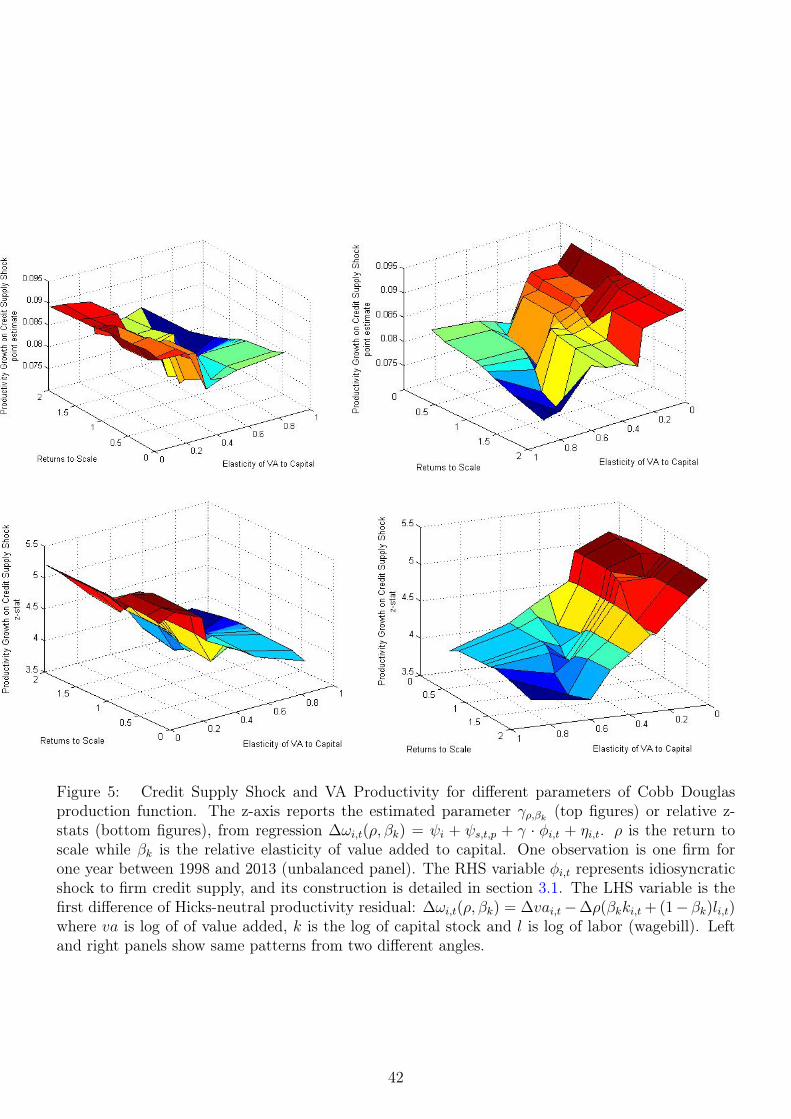
Figure 5: Credit Supply Shock and VA Productivity for different parameters of Cobb Douglasproduction function. The z-axis reports the estimated parameter γρ,βk (top figures) or relative z-stats (bottom figures), from regression ∆ωi,t(ρ, βk) = ψi + ψs,t,p + γ · φi,t + ηi,t. ρ is the return toscale while βk is the relative elasticity of value added to capital. One observation is one firm forone year between 1998 and 2013 (unbalanced panel). The RHS variable φi,t represents idiosyncraticshock to firm credit supply, and its construction is detailed in section 3.1. The LHS variable is thefirst difference of Hicks-neutral productivity residual: ∆ωi,t(ρ, βk) = ∆vai,t−∆ρ(βkki,t + (1− βk)li,t)where va is log of of value added, k is the log of capital stock and l is log of labor (wagebill). Leftand right panels show same patterns from two different angles.

42

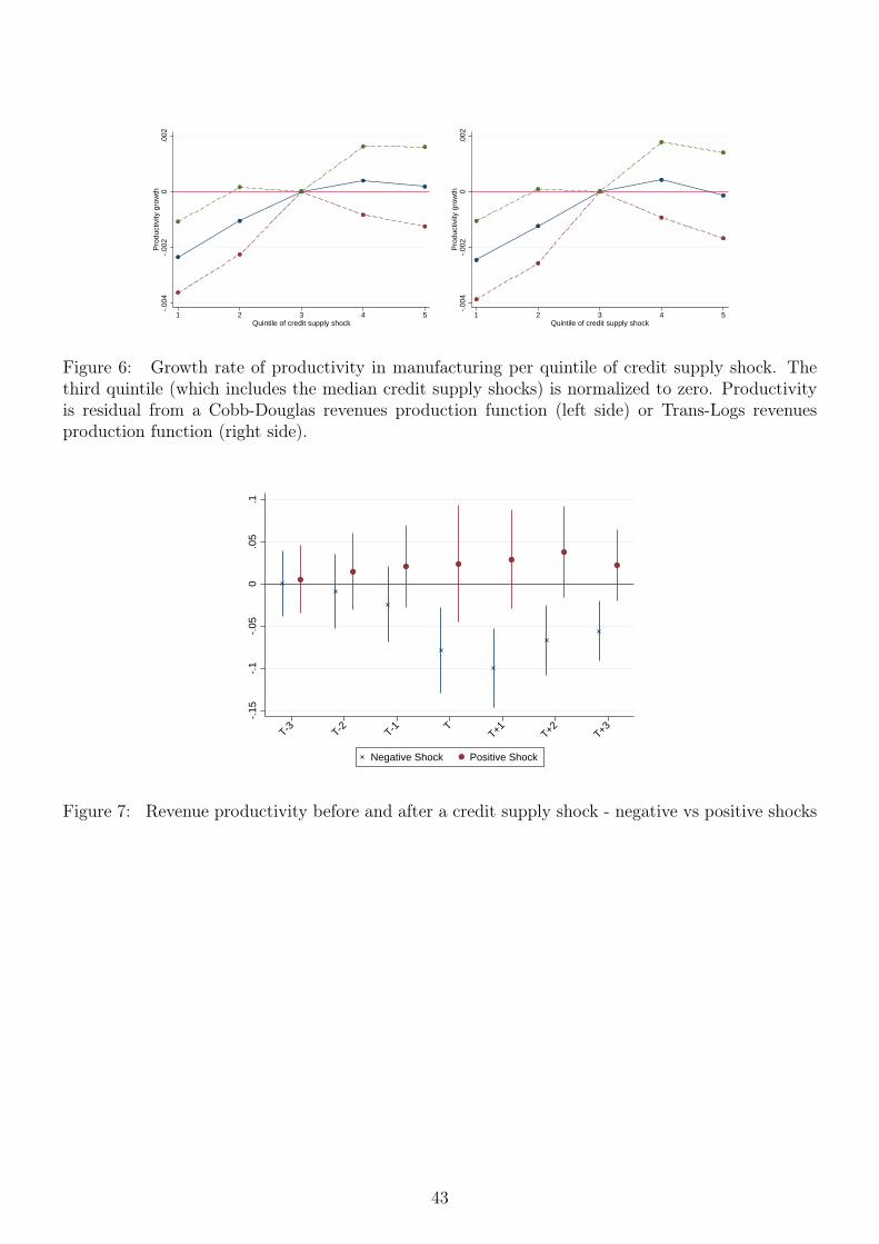
-.00

4-.

002

0.0

02P

rodu

ctiv

ity g

row

th

1 2 3 4 5Quintile of credit supply shock

-.00

4-.

002

0.0

02P

rodu

ctiv

ity g

row

th

1 2 3 4 5Quintile of credit supply shock

Figure 6: Growth rate of productivity in manufacturing per quintile of credit supply shock. Thethird quintile (which includes the median credit supply shocks) is normalized to zero. Productivityis residual from a Cobb-Douglas revenues production function (left side) or Trans-Logs revenuesproduction function (right side).

-.15

-.1

-.05

0.0

5.1

T-3 T-2 T-1 TT+1 T+2 T+3

Negative Shock Positive Shock

Figure 7: Revenue productivity before and after a credit supply shock - negative vs positive shocks

43

Tables

Table 1: Descriptive Statistics - main firm-level variables

VARIABLE Mean Std. Dev. Median N Mean Std. Dev. Median NAll Industries Manufacturing

Value Added 5,312 33,819 1,641 656,960 5,409 21,699 1,943 347,990Net Revenues 27,073 156,638 8,813 656,960 25,351 164,054 8,209 347,990Wagebill 3,377 19693.9 1,062 656,960 3,466 13452.4 1,299 347,990Capital Stock 8,636 153,346 1,545 656,960 7,111 40,357 2,058 347,990Intermediate Inputs 21,888 137,390 6,873 656,960 20,057 150,610 6,119 347,990Credit Granted 7,924 3,6445 2,737 650,664 8,039 29,760 3,013 345,700Employees 80 472 28 656,960 79 269 35 347,990

Notes: One observation is one firm for one year, between 1998 and 2013 (unbalanced panel). All variables(except for number of employees) are expressed as thousands of 2010 euros using sector-level deflators fromnational accounts.Source: CADS and Credit Register.

Table 2: Credit, Inputs and Outputs response to Credit Supply Shocks

VARIABLES Credit Value Net Capital Wagebill Number of Intermediate( in delta Log) Received Added Revenues Stock Employees Inputs

(1) (2) (3) (4) (5) (6) (7)All Industries

φi,t 0.949*** 0.123*** 0.0474*** 0.0619*** 0.0154* 0.00608 0.0220*(0.0196) (0.0162) (0.0109) (0.0128) (0.00926) (0.00889) (0.0114)

Observations 609,195 656,960 656,960 656,960 656,960 656,960 656,960R2 0.239 0.224 0.302 0.259 0.324 0.319 0.302

Manufacturing

φi,t 0.966*** 0.134*** 0.0436*** 0.0610*** 0.00388 -0.00892 0.00716(0.0253) (0.0201) (0.0143) (0.0169) (0.0116) (0.0108) (0.0152)

Observations 324,926 347,990 347,990 347,990 347,990 347,990 347,990R2 0.224 0.241 0.309 0.253 0.326 0.317 0.308

Notes: Results of estimating model:

∆xi,t = ψi + ψs,t,p + γ · φi,t + ηi,t

One observation is one firm for one year between 1998 and 2013 (unbalanced panel). ∆xi,t is the delta-logof the variable described on top of each column, in real terms (2010 euros). φi,t is an idiosyncratic shockto firm credit supply, whose construction is detailed in section 3.1. Firm FEs and province×industry×yearFEs are included. Singleton observations are dropped. A 1% increase in φi,t is the supply shock needed toincrease the credit granted to firm i by 1%. The first column has less observation because some firms mighthave no credit granted in one year, and therefore delta logs are ill-defined. Standard errors (in parentheses)are clustered at firm level. *** p<0.01, ** p<0.05, * p<0.1

44

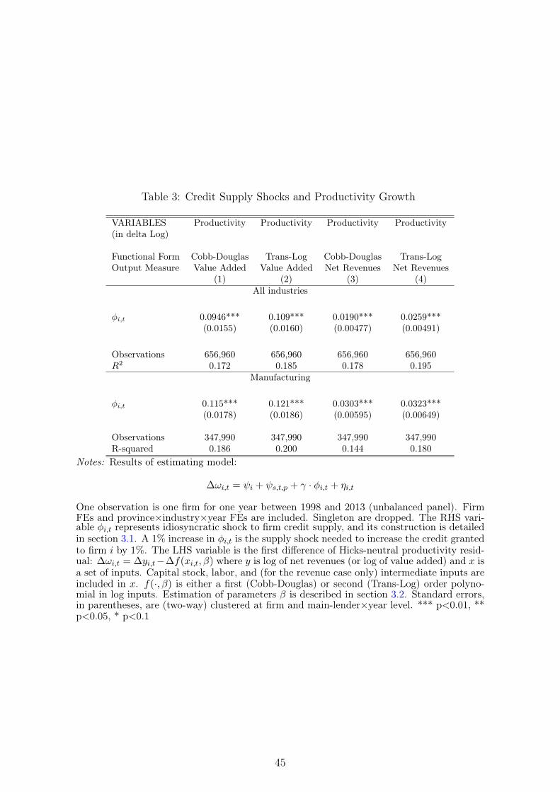
Table 3: Credit Supply Shocks and Productivity Growth

VARIABLES Productivity Productivity Productivity Productivity(in delta Log)

Functional Form Cobb-Douglas Trans-Log Cobb-Douglas Trans-LogOutput Measure Value Added Value Added Net Revenues Net Revenues

(1) (2) (3) (4)All industries

φi,t 0.0946*** 0.109*** 0.0190*** 0.0259***(0.0155) (0.0160) (0.00477) (0.00491)

Observations 656,960 656,960 656,960 656,960R2 0.172 0.185 0.178 0.195

Manufacturing

φi,t 0.115*** 0.121*** 0.0303*** 0.0323***(0.0178) (0.0186) (0.00595) (0.00649)

Observations 347,990 347,990 347,990 347,990R-squared 0.186 0.200 0.144 0.180

Notes: Results of estimating model:

∆ωi,t = ψi + ψs,t,p + γ · φi,t + ηi,t

One observation is one firm for one year between 1998 and 2013 (unbalanced panel). FirmFEs and province×industry×year FEs are included. Singleton are dropped. The RHS vari-able φi,t represents idiosyncratic shock to firm credit supply, and its construction is detailedin section 3.1. A 1% increase in φi,t is the supply shock needed to increase the credit grantedto firm i by 1%. The LHS variable is the first difference of Hicks-neutral productivity resid-ual: ∆ωi,t = ∆yi,t−∆f(xi,t, β) where y is log of net revenues (or log of value added) and x isa set of inputs. Capital stock, labor, and (for the revenue case only) intermediate inputs areincluded in x. f(·, β) is either a first (Cobb-Douglas) or second (Trans-Log) order polyno-mial in log inputs. Estimation of parameters β is described in section 3.2. Standard errors,in parentheses, are (two-way) clustered at firm and main-lender×year level. *** p<0.01, **p<0.05, * p<0.1

45

Table4:

CreditSu

pply

Shocks

andProdu

ctivity

Growth:Rob

ustness-Cob

b-Dou

glas

Revenue

Produ

ctivity

VARIA

BLE

SProdu

ctivity

Produ

ctivity

Produ

ctivity

Produ

ctivity

Produ

ctivity

Produ

ctivity

Produ

ctivity

Produ

ctivity

Produ

ctivity

Produ

ctivity

(delta

Logs)

Mod

elBaseline

Firm

Impo

rtan

tPoo

led

Alterna

tive

Match

Split

4Digits

End

ogenou

sCost

Con

trols

Borrowers

Estim

ator

FEsstructure

Con

trols

Sample

Sector

Exit

Share

(1)

(2)

(3)

(4)

(5)

(6)

(7)

(8)

(9)

(10)

AllIndu

stries

φi,t

0.0190***

0.0248***

0.0182***

0.0131***

0.0171***

0.0234***

0.0197***

0.0278***

0.0166***

0.0256***

(0.00477)

(0.00534)

(0.00540)

(0.00327)

(0.00471)

(0.00604)

(0.00503)

(0.00585)

(0.00465)

(0.00736)

Observation

s656,960

483,665

521,741

656,960

656,960

656,960

656,960

587,873

656,960

545,162

R-squ

ared

0.178

0.184

0.192

0.006

0.096

0.178

0.178

0.272

0.177

0.185

Man

ufacturing

φi,t

0.0303***

0.0362***

0.0330***

0.0188***

0.0321***

0.0331***

0.0292***

0.0401***

0.0295***

0.0537***

(0.00595)

(0.00657)

(0.00698)

(0.00443)

(0.00600)

(0.00739)

(0.00633)

(0.00731)

(0.00639)

(0.0104)

Observation

s347,990

262,308

280,346

347,990

347,990

347,990

347,990

309,887

347,990

291,071

R-squ

ared

0.144

0.153

0.150

0.004

0.071

0.144

0.144

0.259

0.166

0.161

Notes:Results

ofestimatingmod

el:

∆ωi,t

=ψi+ψs,t,p

+γ·φ

i,t

+η i,t

One

observationis

onefirm

foron

eyear

betw

een1998

and2013

(unb

alan

cedpa

nel).Firm

FEsan

dprovince×indu

stry×year

FEsareinclud

ed.Sing

letons

aredrop

ped.

φi,tisan

idiosyncraticshockto

creditsupp

ly,w

hose

construction

isdetailedin

section3.1.

A1%

increase

inφi,tisthesupp

lyshockneeded

toincrease

thecreditgran

ted

tofirmiby

1%.The

LHSvariab

leis

thefirst

diffe

renceof

prod

uctivity

residu

al:

∆ωi,t

=∆y i,t−βk·∆

ki,t−βl·∆

l i,t−βm·∆

mi,twhereyis

logof

netrevenu

es,k

islogof

capitalstock,lis

labo

r(m

easuredby

logof

wagebill)an

dm

islogof

interm

ediate

inpu

ts.Estim

ationof

parametersβis

describe

din

section3.2.

Colum

n(2)

addasetof

lagged

controls

toba

selin

especification

:po

lyno

mialin

size

(assets)

andtheratios

ofvaluead

ded,

liquidity,cash

flow

andba

nkde

btto

assets.It

exclud

esob

servationwithmissing

orzero

values

foran

ycontrolvariab

le.Colum

n(3)exclud

esan

yfirm

that,at

anypo

intin

time,

was

therecipientof

morethan

1%of

the

totalc

reditof

anyfin

ancial

interm

ediary.Colum

n(4)exclud

esfirm

FEs.

Colum

n(5)includ

esad

ditively

firm

FEs,

prov

ince

FEs,

year

FEs,

andindu

stry

FEs.

Colum

n(6)uses

analternativemeasure

ofcredit

supp

lyshocks

which

controlformatch-spe

cific

covariates,seesection3.1.

Colum

n(7)uses

analternativecredit

supp

lyshocks

estimated

witha“splitsample”

proced

ure,

inorderto

controlfor

finitesamplebiases.Colum

n(8)uses

a4-digits

(ratherthan

2)indu

stry

defin

ition.

Itisestimated

over

less

observations

becauseof

moresing

letons.Colum

n(9)estimateprod

uctivity

allowingforendo

geno

usfirm

exit,as

inOlley&

Pakes

(1996).Colum

n(10)

estimates

prod

uctivity

usingthecost

sharemetho

d.It

contains

less

observationbe

causeservices

andmaterials

areenteredad

ditively,a

ndno

tallfi

rmsrepo

rtbo

thinterm

ediates.

Stan

dard

errors,inpa

rentheses,

are(two-way

)clusteredat

firm

andmain-lend

er×year

level.***p<

0.01,*

*p<

0.05,*

p<0.1

46

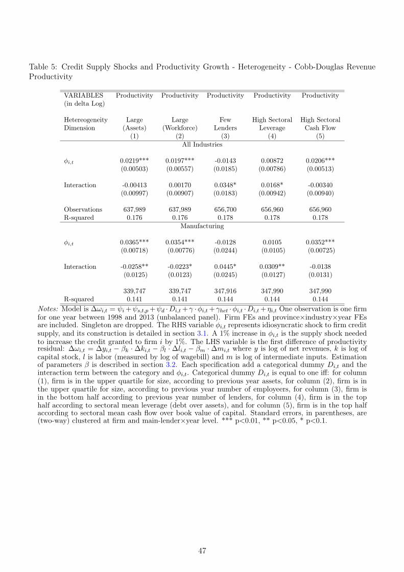
Table 5: Credit Supply Shocks and Productivity Growth - Heterogeneity - Cobb-Douglas RevenueProductivity

VARIABLES Productivity Productivity Productivity Productivity Productivity(in delta Log)

Hetereogeneity Large Large Few High Sectoral High SectoralDimension (Assets) (Workforce) Lenders Leverage Cash Flow

(1) (2) (3) (4) (5)All Industries

φi,t 0.0219*** 0.0197*** -0.0143 0.00872 0.0206***(0.00503) (0.00557) (0.0185) (0.00786) (0.00513)

Interaction -0.00413 0.00170 0.0348* 0.0168* -0.00340(0.00997) (0.00907) (0.0183) (0.00942) (0.00940)

Observations 637,989 637,989 656,700 656,960 656,960R-squared 0.176 0.176 0.178 0.178 0.178

Manufacturing

φi,t 0.0365*** 0.0354*** -0.0128 0.0105 0.0352***(0.00718) (0.00776) (0.0244) (0.0105) (0.00725)

Interaction -0.0258** -0.0223* 0.0445* 0.0309** -0.0138(0.0125) (0.0123) (0.0245) (0.0127) (0.0131)

339,747 339,747 347,916 347,990 347,990R-squared 0.141 0.141 0.144 0.144 0.144

Notes: Model is ∆ωi,t = ψi +ψs,t,p +ψd ·Di,t+γ ·φi,t +γhet ·φi,t ·Di,t + ηi,t One observation is one firmfor one year between 1998 and 2013 (unbalanced panel). Firm FEs and province×industry×year FEsare included. Singleton are dropped. The RHS variable φi,t represents idiosyncratic shock to firm creditsupply, and its construction is detailed in section 3.1. A 1% increase in φi,t is the supply shock neededto increase the credit granted to firm i by 1%. The LHS variable is the first difference of productivityresidual: ∆ωi,t = ∆yi,t − βk ·∆ki,t − βl ·∆li,t − βm ·∆mi,t where y is log of net revenues, k is log ofcapital stock, l is labor (measured by log of wagebill) and m is log of intermediate inputs. Estimationof parameters β is described in section 3.2. Each specification add a categorical dummy Di,t and theinteraction term between the category and φi,t. Categorical dummy Di,t is equal to one iff: for column(1), firm is in the upper quartile for size, according to previous year assets, for column (2), firm is inthe upper quartile for size, according to previous year number of employeers, for column (3), firm isin the bottom half according to previous year number of lenders, for column (4), firm is in the tophalf according to sectoral mean leverage (debt over assets), and for column (5), firm is in the top halfaccording to sectoral mean cash flow over book value of capital. Standard errors, in parentheses, are(two-way) clustered at firm and main-lender×year level. *** p<0.01, ** p<0.05, * p<0.1.

47

Table 6: Exposure to Interbank Market and Productivity Growth

VARIABLES Productivity Productivity Productivity Productivity(in delta Log)

Functional Form Cobb-Douglas Trans-Log Cobb-Douglas Trans-LogOutput Measure Value Added Value Added Net Revenues Net Revenues

(1) (2) (3) (4)All Industries

ITBKi,2006 -0.0477** -0.0574** -0.0172** -0.0222***(0.0239) (0.0257) (0.00757) (0.00781)

Observations 110,746 110,746 110,746 110,746R2 0.112 0.117 0.101 0.122

Manufacturing

ITBKi,2006 -0.0802** -0.106*** -0.00837 -0.0178*(0.0329) (0.0361) (0.00960) (0.0106)

Observations 58,191 58,191 58,187 58,187R2 0.134 0.143 0.086 0.113

Notes: Model is ∆ωi,t = ψs,t,p + γ · ITBKi,2006 + ηi,t One observation is one firm for one year between2007 and 2009 (unbalanced panel). Province×industry×year FEs are included. Singleton are dropped.The RHS variable ITBKi,2006 is the weighted average of firm’s i lenders’ liability on the interbankmarket over assets in 2006. The LHS variable is the first difference of Hicks-neutral productivityresidual: ∆ωi,t = ∆yi,t −∆f(xi,t, β) where y is log of net revenues (or log of value added) and x is aset of inputs. Capital stock, labor, and (for the revenue case only) intermediate inputs are includedin x. f(·, β) is either a first (Cobb-Douglas) or second (Trans-Log) order polynomial in log inputs.Estimation of parameters β is described in section 3.2. Standard errors (in parentheses) are clusteredat firm level. *** p<0.01, ** p<0.05, * p<0.1.

48

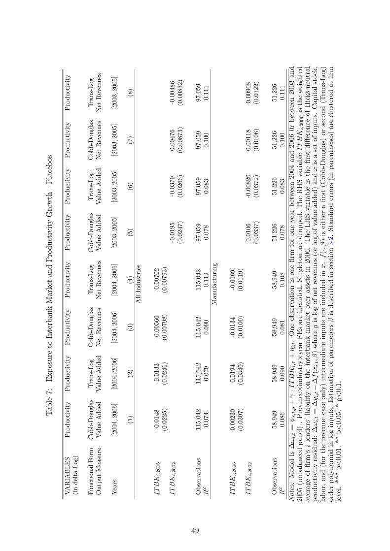
Table7:

Exp

osureto

Interban

kMarketan

dProdu

ctivity

Growth

-Placebo

s

VARIA

BLE

SProdu

ctivity

Produ

ctivity

Produ

ctivity

Produ

ctivity

Produ

ctivity

Produ

ctivity

Produ

ctivity

Produ

ctivity

(indeltaLo

g)

Function

alFo

rmCob

b-Dou

glas

Trans-Log

Cob

b-Dou

glas

Trans-Log

Cob

b-Dou

glas

Trans-Log

Cob

b-Dou

glas

Trans-Log

Outpu

tMeasure

Value

Add

edValue

Add

edNet

Revenues

Net

Revenue

sValue

Add

edValue

Add

edNet

Revenues

Net

Revenues

Years

[200

4,2

006]

[200

4,2

006]

[200

4,2

006]

[2004,

2006]

[2003,

2005]

[2003,2

005]

[2003,2

005]

[2003,

2005]

(1)

(2)

(3)

(4)

(5)

(6)

(7)

(8)

AllIndu

stries

ITBKi,2006

-0.0148

-0.0133

-0.00560

-0.00702

(0.0225)

(0.0246)

(0.00798)

(0.00793)

ITBKi,2002

-0.0195

-0.0379

0.00476

-0.00486

(0.0247)

(0.0266)

(0.00873)

(0.00832)

Observation

s115,042

115,042

115,042

115,042

97,059

97,059

97,059

97,059

R2

0.074

0.079

0.090

0.112

0.078

0.083

0.100

0.111

Man

ufacturing

ITBKi,2006

0.00230

0.0194

-0.0134

-0.0169

(0.0307)

(0.0340)

(0.0100)

(0.0119)

ITBKi,2002

0.0106

-0.00820

0.00118

0.00908

(0.0337)

(0.0372)

(0.0106)

(0.0122)

Observation

s58,949

58,949

58,949

58,949

51,226

51,226

51,226

51,226

R2

0.086

0.090

0.081

0.108

0.078

0.083

0.100

0.111

Not

es:Mod

elis

∆ωi,t

=ψs,t,p

+γ·ITBKi,τ

+η i,t.One

observationis

onefirm

foron

eyear

betw

een2004

and2006

0rbe

tween2003

and

2005

(unb

alan

cedpa

nel).Provinc

e×indu

stry×year

FEsareinclud

ed.Sing

letonaredrop

ped.

The

RHSvariab

leITBKi,2006istheweigh

ted

averag

eof

firm’silend

ers’

liabilityon

theinterban

kmarketover

assets

in20

06.The

LHSvariab

leis

thefirst

diffe

renc

eof

Hicks-neu

tral

prod

uctivity

residu

al:

∆ωi,t

=∆y i,t−

∆f

(xi,t,β

)whe

reyislogof

netrevenu

es(orlogof

valuead

ded)

andxisasetof

inpu

ts.Cap

ital

stock,

labo

r,an

d(for

therevenu

ecase

only)interm

ediate

inpu

tsareinclud

edinx.f

(·,β

)is

either

afirst

(Cob

b-Dou

glas)or

second

(Trans-Log)

orde

rpo

lyno

mialinloginpu

ts.Estim

ationof

parametersβisde

scribe

din

section3.2.

Stan

dard

errors

(inpa

renthe

ses)

areclusteredat

firm

level.

***p<

0.01

,**p<

0.05

,*p<

0.1.

49

Table8:

CreditSu

pply

Shockan

dProdu

ctivity

-Enh

ancing

Activities

VARIA

BLE

SPCspe

rNo.

ofPatents

Patent

R&D

Export

FinCon

i,2010

Man

agem

ent

unitof

Cap

ital

App

lications

Growth

Score

(1)

(2)

(3)

(4)

(5)

(6)

(7)

φi,t

0.80

8***

0.23

8*0.15

2*-1.629

***

2.16

6*(0.289)

(0.128)

(0.085)

(0.594)

(1.116)

φi,t−

10.04

18**

1.75

9**

(0.0197)

(0.883)

Mod

elPan

elPan

elPan

elPan

elPan

elCross

Section

Cross

Section

Observation

s3,63

251

7,16

513

,522

5,991

13,249

506

183

R2

0.96

80.75

70.56

20.87

20.84

30.42

10.020

Not

es:Colum

ns(1)to

(5):

mod

elYi,t

=ψi+ψs,t,p

+γ·φ

i,t

+η i,tOne

observationis

onefirm

foron

eyear

betw

een1999

and20

01(unb

alan

cedpa

nel).Firm

FEsan

dprov

ince×indu

stry×year

FEsareinclud

ed.Sing

letonaredrop

ped.

The

RHS

variab

leφi,trepresents

idiosync

raticshockto

firm

cred

itsupp

ly,an

d(see

section3.1).A

1%increase

inφi,tis

thesupp

lyshockneed

edto

increase

thecred

itgran

tedto

firmiby

1%.RHSvariab

leislagg

edin

column(2)an

d(3).

LHSof

column(1)

isthelogof

numbe

rof

PCspe

r1,00

0eu

rosof

capital.The

LHSvariab

lein

column(2)isthenu

mbe

rof

patent

application

mad

efrom

compa

nyiin

yeart.

Colum

n(3)isthegrow

thrate

ofthenu

mbe

rof

patent

applications

mad

eby

compa

nyiin

yeartversust−

2.Colum

ns(4)an

d(5):

mod

elisDi,t

=ψi+ψt+γ·φi,t+η i,t.Di,tisadu

mmyvariab

letaking

value1iff

firm

iin

yeartha

spo

sitive

investmentin

R&D,c

olum

n(4),or

adu

mmyvariab

letaking

value1iff

firmiin

yeartha

spo

sitive

expo

rtrevenu

es,c

olum

n(5).

Colum

n(6):

linearprob

ability

mod

elisFinCon

i,2010

=ψs,p

+γ·φ

i,2010

+η i.One

observation

ison

efirm

(cross

section).Provinc

e×Indu

stry

fixed

effects

areinclud

ed.FinCon

i,2010isadu

mmytaking

valueon

eiff

firm

irepo

rts“diffi

cultiesto

getexternal

fund

s”as

anim

portan

tor

someh

owim

portan

tob

stacle

toinno

vation

.Num

berof

PCs,

expo

rtactivity,R&D

investments,an

dself-repo

rted

obstacle

toinno

vation

aretakenfrom

INVIN

D.Colum

n(7):

mod

elisMSi,t

=ψ

+γ·φ

i,t

+η i,t.One

observationis

onefirm

observed

foron

eor

twoyears(cross

section).MSi,tis

firmi

overallman

agem

entscoreprov

ided

bytheWorld

Man

agem

entSu

rvey

(Bloom

&Van

Reene

n,2007).

Ittakesvaluefrom

1-5.

Stan

dard

errors

(inpa

renthe

ses)

areclusteredat

firm

level.

***p<

0.01

,**

p<0.05,*p<

0.1.

Seesection8formore

details.

50

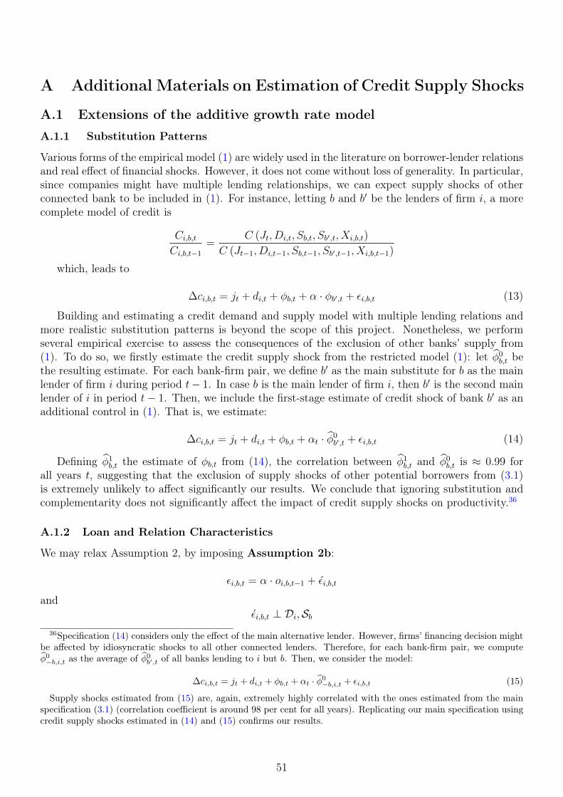
A Additional Materials on Estimation of Credit Supply Shocks

A.1 Extensions of the additive growth rate model

A.1.1 Substitution Patterns

Various forms of the empirical model (1) are widely used in the literature on borrower-lender relationsand real effect of financial shocks. However, it does not come without loss of generality. In particular,since companies might have multiple lending relationships, we can expect supply shocks of otherconnected bank to be included in (1). For instance, letting b and b′ be the lenders of firm i, a morecomplete model of credit is

Ci,b,tCi,b,t−1

=C (Jt, Di,t, Sb,t, Sb′,t, Xi,b,t)

C (Jt−1, Di,t−1, Sb,t−1, Sb′,t−1, Xi,b,t−1)

which, leads to

∆ci,b,t = jt + di,t + φb,t + α · φb′,t + εi,b,t (13)

Building and estimating a credit demand and supply model with multiple lending relations andmore realistic substitution patterns is beyond the scope of this project. Nonetheless, we performseveral empirical exercise to assess the consequences of the exclusion of other banks’ supply from(1). To do so, we firstly estimate the credit supply shock from the restricted model (1): let φ0

b,t bethe resulting estimate. For each bank-firm pair, we define b′ as the main substitute for b as the mainlender of firm i during period t− 1. In case b is the main lender of firm i, then b′ is the second mainlender of i in period t− 1. Then, we include the first-stage estimate of credit shock of bank b′ as anadditional control in (1). That is, we estimate:

∆ci,b,t = jt + di,t + φb,t + αt · φ0b′,t + εi,b,t (14)

Defining φ1b,t the estimate of φb,t from (14), the correlation between φ1

b,t and φ0b,t is ≈ 0.99 for

all years t, suggesting that the exclusion of supply shocks of other potential borrowers from (3.1)is extremely unlikely to affect significantly our results. We conclude that ignoring substitution andcomplementarity does not significantly affect the impact of credit supply shocks on productivity.36

A.1.2 Loan and Relation Characteristics

We may relax Assumption 2, by imposing Assumption 2b:

εi,b,t = α · oi,b,t−1 + εi,b,t

andεi,b,t ⊥ Di,Sb

36Specification (14) considers only the effect of the main alternative lender. However, firms’ financing decision mightbe affected by idiosyncratic shocks to all other connected lenders. Therefore, for each bank-firm pair, we computeφ0−b,i,t as the average of φ0b′,t of all banks lending to i but b. Then, we consider the model:

∆ci,b,t = jt + di,t + φb,t + αt · φ0−b,i,t + εi,b,t (15)

Supply shocks estimated from (15) are, again, extremely highly correlated with the ones estimated from the mainspecification (3.1) (correlation coefficient is around 98 per cent for all years). Replicating our main specification usingcredit supply shocks estimated in (14) and (15) confirms our results.

51

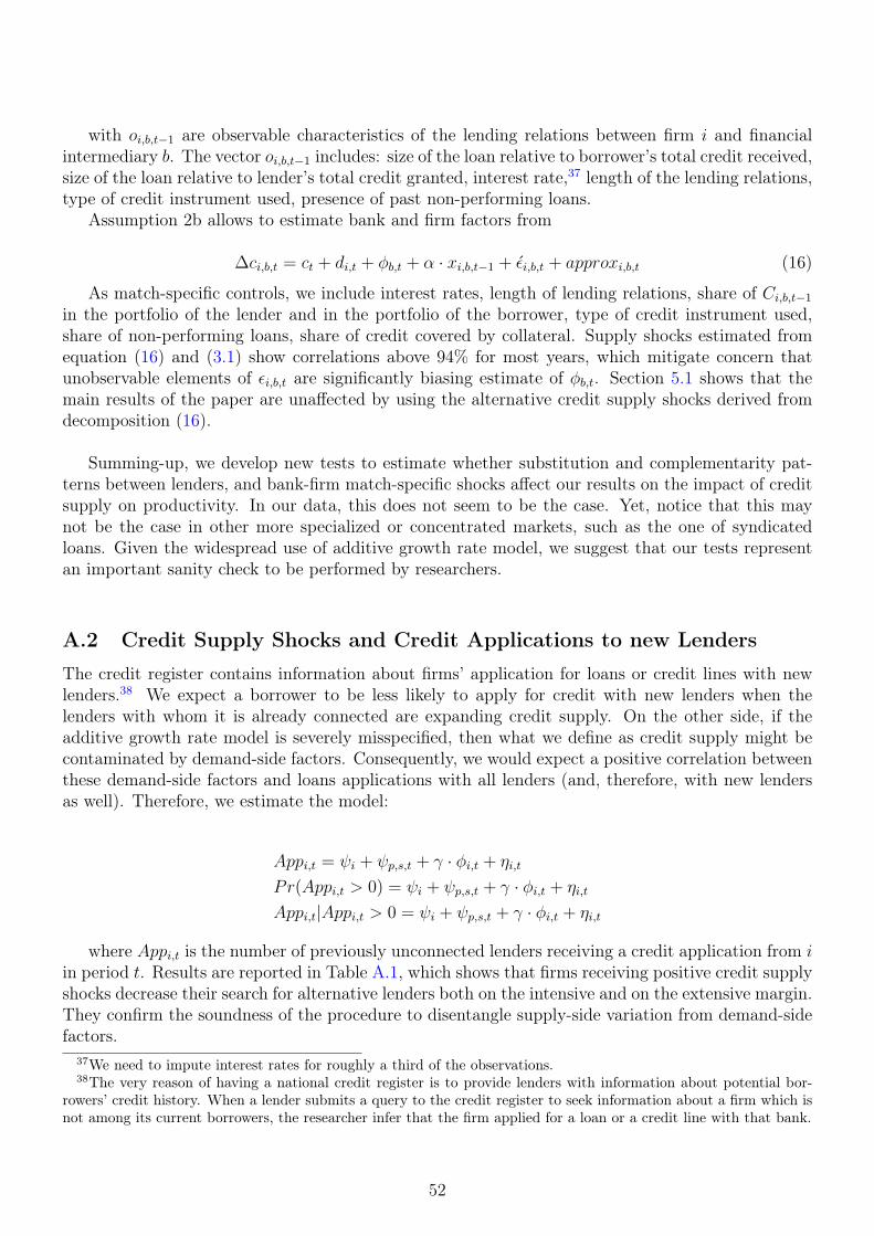
with oi,b,t−1 are observable characteristics of the lending relations between firm i and financialintermediary b. The vector oi,b,t−1 includes: size of the loan relative to borrower’s total credit received,size of the loan relative to lender’s total credit granted, interest rate,37 length of the lending relations,type of credit instrument used, presence of past non-performing loans.

Assumption 2b allows to estimate bank and firm factors from

∆ci,b,t = ct + di,t + φb,t + α · xi,b,t−1 + εi,b,t + approxi,b,t (16)

As match-specific controls, we include interest rates, length of lending relations, share of Ci,b,t−1in the portfolio of the lender and in the portfolio of the borrower, type of credit instrument used,share of non-performing loans, share of credit covered by collateral. Supply shocks estimated fromequation (16) and (3.1) show correlations above 94% for most years, which mitigate concern thatunobservable elements of εi,b,t are significantly biasing estimate of φb,t. Section 5.1 shows that themain results of the paper are unaffected by using the alternative credit supply shocks derived fromdecomposition (16).

Summing-up, we develop new tests to estimate whether substitution and complementarity pat-terns between lenders, and bank-firm match-specific shocks affect our results on the impact of creditsupply on productivity. In our data, this does not seem to be the case. Yet, notice that this maynot be the case in other more specialized or concentrated markets, such as the one of syndicatedloans. Given the widespread use of additive growth rate model, we suggest that our tests representan important sanity check to be performed by researchers.

A.2 Credit Supply Shocks and Credit Applications to new Lenders

The credit register contains information about firms’ application for loans or credit lines with newlenders.38 We expect a borrower to be less likely to apply for credit with new lenders when thelenders with whom it is already connected are expanding credit supply. On the other side, if theadditive growth rate model is severely misspecified, then what we define as credit supply might becontaminated by demand-side factors. Consequently, we would expect a positive correlation betweenthese demand-side factors and loans applications with all lenders (and, therefore, with new lendersas well). Therefore, we estimate the model:

Appi,t = ψi + ψp,s,t + γ · φi,t + ηi,t

Pr(Appi,t > 0) = ψi + ψp,s,t + γ · φi,t + ηi,t

Appi,t|Appi,t > 0 = ψi + ψp,s,t + γ · φi,t + ηi,t

where Appi,t is the number of previously unconnected lenders receiving a credit application from iin period t. Results are reported in Table A.1, which shows that firms receiving positive credit supplyshocks decrease their search for alternative lenders both on the intensive and on the extensive margin.They confirm the soundness of the procedure to disentangle supply-side variation from demand-sidefactors.

37We need to impute interest rates for roughly a third of the observations.38The very reason of having a national credit register is to provide lenders with information about potential bor-

rowers’ credit history. When a lender submits a query to the credit register to seek information about a firm which isnot among its current borrowers, the researcher infer that the firm applied for a loan or a credit line with that bank.

52

A.3 Which factors shape credit supply?

Jensen & Johannesen (2016) show that Danish banks entering the 2007-2008 financial crisis withweaker balance sheets declined sharply their lending to retail customers, depressing their consump-tion. They use a proxy for liquidity in 2007 (loans over deposits) to measure balance sheet strength.To provide additional evidence that our measure of credit supply captures bank-level shocks, for eachyear t between 2007 and 2009 (credit crunch) we estimate the linear model:

φb,t = φt + γ ·(

Loans

Deposits

)b,2007

+ ηb,t

Results are presented in Column (1) of Table A.10: banks with lower liquidity at the beginning ofthe credit crunch, decreased more their credit supply. We follow Jensen & Johannesen (2016) and relyon 2007 balance sheet to construct the RHS variable. Results are robust to use 2006 values. Column(2) of the same table uses the capital adequacy ratio (the ratio of bank capital to risk-weighed assets)as an alternative measure of financial strength: better capitalized banks decreased less their creditsupply during the credit crunch.

During the Europe sovereign debt crisis, the spread on bonds issued by Italian government (andother southern European countries) increased sharply. Investors responded by acquiring more of theseassets, “crowding out” credit to private non-financial corporation (Broner et al. , 2014). Therefore,for each year between 2010 and 2013, we estimate the model:

φb,t = φt + γ ·∆(Sovereign

Assets

)b,t

+ ηb,t

where(SovereignAssets

)b,t

is the share of sovereign bonds on the total assets of bank b. Results arepresented in column (3) of of Table A.10: banks increasing more their exposure to sovereign debtdecreased their credit supply to corporate borrowers.

After an M&A episode, acquired banks generally reduce (in the short-run) their supply of creditto pre-existing borrowers (Buono & Formai, 2013). Following this intuition, we estimate the model:

φi,t = φi + φt,p,s + γ ·MAi,t + ηi,t

where φi,t is the credit supply shock experienced by firm i and MAi,t is the share of i ’s previousperiod lenders which are being acquired by another financial institution. Results are presented incolumn (4) of Table A.10: credit supply is negatively affected by lenders’ M&A episodes.

The collection of results presented in this section, being consistent with the relevant literature,provide additional support to our measure of credit supply shocks.

B Production with Heterogeneous Credit Constraints

B.1 Main model

Firm i, operates in sector s and province p. For simplicity, we omit the subscript s, although allparameters, are industry-specific. In each year t, firm combines capital, labor and materials togenerate revenues:

Yi,t = exp{ωi,t}F (Li,t, Ki,t,Mi,t, β) (17)

53

or value added

V Ai,t = exp{ωi,t}F (Li,t, Ki,t, β)

As it is common in the literature (Olley & Pakes, 1996) we assume that productivity can bedecomposed into a structural component and an error term:

ωi,t = ωi,t + εYi,t

ωi,t is correlated over time and it is known by the firm before starting production. Therefore, itaffects inputs acquisition and other firm decisions. εYi,t is an iid shock, which takes place after inputdecisions have been made and does not convey information about future productivity. It is oftenreferred as measurement error of output, or “pure luck”.

Capital accumulationCapital stock is accumulated according to the usual law of motion:

Ki,t = Ii,t + (1− δt)Ki,t−1

PricesFirms are price-takers on the input markets. Prices of materials are assumed to be shaped by

national prices of inputs and by local inflation shocks (measured by local CPI):

PMp,t = PM

t · P (cpip,t)

we do not observe firm level or local level prices of intermediate inputs, so we need to assume aform for P (·).39

Variable Profits and Utility FunctionWe focus the discussion on revenue productivity. The value added case is a straightforward sim-

plification.40 Variable profits are:

π(Ki,t, Li,t, ωi,t, wt, P

Mp,t , ε

Yi,t

)=

= exp{ωi,t + εYi,t}F (Li,t, Ki,t,Mi,t, β)− wtLi,t −Mi,tPMp,t

The firm maximizes owner’s utility from the dividend stream Divi,t:

u(Divi,t, εUt ) + E

[∑τ>t

(1

1 +R)τ−tu(Divi,τ , ε

Uτ )

]

Credit Supply ShocksAt the beginning of the period, firm i is connected to a subset of the banks operating in the

country, Bi,t−1. Each bank “experience” a credit supply shock φb,t. Firm i receive a credit supplyshock equal to φi,t =

∑b∈Bi,t−1

φb,t · wcb,i,t−1 where weights are proportional to the share of credit

39See section 2.40For a discussion see Ackerberg et al. (2015) and De Loecker & Scott (2016).

54

received from firm i from each lender in previous period.

We assume Bi,t and {wcb,i,t−1} evolve exogenously, while the quantity of debt is endogenouslychosen. In section 6 we exploit a natural experiment to control for assortative matching betweenborrowers and lenders and we show that our empirical results hold.

Budget and Credit constraintsFirm faces a budget constraints:

Divi,t +Ki,t +Bi,t−1 (1 + ri,t) + Adj(Li,t, Li,t−1, Ki,t, Ki,t−1, Jt, ε

adji,t

)=

= πi,t +Bi,t + (1− δt)Ki,t−1

where Bi,t is the quantity of euros borrowed, Adj (·) are adjustment costs for labor and capital,Jt is the set of all industry-wide state variables.

credit constraint

Bi,t ≤ Ki,t−1 · Γ (Bi,t−1, φi,t, ωi,t, Jt, )

we also allow single inputs to have specific financially-generated constraints.

Mi,t ≤ Ki,t−1 · ΓM (Bi,t−1, φi,t, ωi,t, Jt)

Ki,t ≤ Ki,t−1 · ΓK (Bi,t−1, φi,t, ωi,t, Jt)

Li,t ≤ Ki,t−1 · ΓL (Bi,t−1, φi,t, ωi,t, Jt)

furthermore, we assume the function ΓM is increasing in its second and third arguments.

The presence of general credit constraints does not imply that intermediate inputs are constrained.However, we want to allow for this possibility, since firms might need to pay in advance part of thematerial inputs and availability of credit (especially credit lines) might limit their ability to do so.Whether or not an input is effectively contained by availability of external funds depends on therelative cash cycle. For instance, capital investments might be more sensitive to credit availabilitythan labor because they have to be paid fully in advance. However, while firms make financial andreal decision in continuous time (or every day), our model discretize time in yearly periods, as it iscommonly do by the literature because balance-sheets data are available at yearly frequency. Allow-ing for input-specific constraints is a way to partly reconcile the model with reality.

TimingAt the beginning of the period firms observe ωi,t εKi,t ε

adji,t φi,t and all elements of Jt (like εut and

cpip,t ). Then, it choose jointly Bi,t and all inputs Ki,t, Li,t and Mi,t. Firms do not observe the nontransmitted error εYi,t until the end of the period. When the random shock εYi,t is realized, Divi,t is setas residual from the budget constraint and it is consumed.

Law of Motion

55

The non transmitted shock εYi,t is pure luck and, therefore, it is i.i.d and independent of any othercomponent of the model. Without loss of generality, we set E[exp{εYi,t}] = 1. The law of motionof all other shocks εi,t is left unrestricted. However, notice that the absence of any shock directlyaffecting intermediate inputs is essential for identification.

Following the tradition of the control function, we impose a law of motion for productivity. Thatis,

E [ωi,t|It−1] = E [ωi,t|ωi,t−1, φi,t−1, Jt−1] (18)

where It−1 is firm’s information set at time t− 1. Assumption 18 relaxes the classical Markovianstructure by allowing credit supply to affect productivity dynamics.

Furthermore, defining:

ζi,t := ωi,t − E [ωi,t|It−1] (19)

and

ζφi,t := φi,t − E [φi,t|φi,t−1] (20)

we assume ζφi,t is independent of all ε’s.

Demand for intermediate inputsThe optimal quantity of intermediate input is

M∗ (Ki,t, Li,t, Ki,t−1ωi,t, Jt, Bi,t−1, PMp,t

)=

min{Munc(Ki,t, Li,t, ωi,t, P

Mp,t

);Ki,t−1 · ΓM (Bi,t−1, φi,t, ωi,t, Jt, )}

where Munc solves

∂F (Li,t, Ki,t,M, β)

∂Mexp{ωi,t} = PM

p,t

under assumptions above,41 M∗ is increasing in productivity for each level of the other factors.Therefore, ∃ an unknown function M−1 such that:

ωi,t = M−1 (Ki,t, Li,t, Ki,t−1, φi,t, cpip,t, Jt)

which allows to write

Yi,t = exp{εYi,t}F (Li,t, Ki,t,Mi,t, β) exp{M−1 (Ki,t, Li,t, Ki,t−1, φi,t, cpip,t, Jt)}41Formally, we assume that M is chosen within a set AM such that F (K,L, ·) is increasing in its last argument for

each value of K and L. Then, Munc is increasing in ω by Topkis theorem. This is trivially true for the Cobb Douglascase, as long as K > 0 and L > 0.

56

therefore, for some unknown function Ψ

Yi,t = exp{εYi,t}Ψ (Li,t, Ki,t,Mi,t, Ki,t−1, φi,t, cpip,t, Jt) (21)

B.1.1 Estimation of the Production Function

We aim at estimating the shape of the production function F (), in order to back out productivityresidual and investigate the joint dynamics of credit supply and productivity. Firstly, we write themain equations in logarithmic terms. Variables in logs are indicated by lowercase letters.

Revenues are:

yi,t = ωi,t + εYi,t + f (li,t, ki,t,mi,t, β) (22)

where f(·) is known up to the parameter β, which we aim to estimate. Revenues, can also bewritten as

yi,t = Ψ (li,t, ki,t,mi,t, ki,t−1, φi,t, cpip,t, Jt) + εYi,t (23)

for some unknown function Ψ. Following Ackerberg et al. (2015), we estimate the modelin two stages. In the first stage we purge the output from the noise εYi,t. We estimate Ψ asEt [yi,t|li,t, ki,t,mi,t, ki,t−1, φi,t, cpip,t].42

From equation (18) we can write

ωi,t = gt (ωi,t−1, φi,t−1) + ζi,t

with gt unknown.

By definition, we have

E[ζi,t + εYi,t|It−1

]= 0

therefore,

E [yi,t − f (li,t, ki,t,mi,t, β)− gt (Ψi,t−1 − f (li,t−1, ki,t−1,mi,t−1, β) , φi,t−1) |It−1] = 0

leading to the moment condition42 E[yi,t|xi,t, Jt] = φ(xi,t, Jt) for some unknown function φ, which we approximate as a third order polynomial in

xi,t plus year fixed effects. We follow this approximation procedure through the paper.

57

E

Ψi,t − f (li,t, ki,t,mi,t, β)−+gt (Ψi,t−1 − f (li,t−1, ki,t−1,mi,t−1, β) , φi,t−1)

|

li,t−1invi,t−1Ψi,t−1mi,t−1..

= 0 (24)

Moments (24) allow joint estimation of the structural parameter β and of the unknown functiongt.43

We parametrize f(·) as either linear (Cobb-Douglas) or quadratic (Trans-Log) in logs. These twofunctions can be seen as a first and second order log-linear approximation of any smooth productionfunction F (·). Since our results are extremely similar between Cobb-Douglas and Trans-Log, we donot believe it is useful to add higher order terms. Production functions are industry-specific. Wedrop sectors for which less than 300 firm-year observations are available, because of difficulties inestimating production function with few observations.

The control function approach allows to estimate production function parameters by controllingfor simultaneity bias in the choice of inputs.44 Furthermore, the inclusion of local price shocks cpip,tin the control function overcomes the non-identification results of Gandhi et al. (2011). In ourbaseline specification, we do not include endogenous exit decision in the model. Section 5.1 showsthat such an inclusion does not significantly affect the main results of this paper.

If credit supply affects productivity, then it is correlated with ζi,t. Moreover, φi,t is correlated overtime: in fact, regression of φi,t on φi,t−1 gives a coefficient of ≈ 0.5 if no fixed effect is included and≈ 0.2 if firm fixed effects are included. Furthermore, it affects input acquisition, as documented bysection 4. Therefore, if one excludes credit supply shocks from the model, past inputs are correlatedwith the productivity innovation, and there are no valid instruments to identify the parameter ofinterests.

Results

Table A.2 provides some descriptives for the Cobb-Douglas production function estimates.45 Themean46 elasticity of value added to capital (to labor) is ≈ .17 (≈ .64) for the whole economy and≈ .19 (≈ .62) for manufacturing. The mean elasticity of net revenues to capital (to labor) is ≈ .07(≈ .14) for the whole economy and ≈ .04 (≈ .13) for manufacturing. The mean elasticity of netrevenues to intermediate inputs is ≈ .81 for both manufacturing and all industries.47

43We follow De Loecker & Warzynski (2012) and we perform this second stage in two steps. For each guess aparameter value βguess, we can compute a corresponding ωi,t(βguess). Then, by regressing ωi,t(βguess) on a polynomialin ωi,t−1(βguess) and φi,t−1 plus year fixed effects we get a sample analog of ζ(βguess). We estimate β by minimizingthen sample analog of E [ζ(βguess) · instrumentsi,t−1].

44That is, since more productive firms are likely to acquire more inputs, a simple regression of output on inputsdoes not recover the structural parameters of interest.

45As it is shown in section 5 the relations between productivity and credit does not change if one consider CD orTrans-Log production function, therefore we do not find it useful to analyses in detail the more complicated case.

46We take averages weighted for number of observation in the sample of the main specification.47Under the assumption of single good producers, we can translate these revenue production function estimate into

a quantity production function. The relations depend on the competitive structure of the product market, see, for

58

B.2 An alternative empirical model of production

The credit supply shock φi,t is a weighted average of supply shocks φb,t of the banks connected tofirm i in the previous period. A potential critique of the main model is that it includes credit supplychanges as an element of the level of the constraint faced each period by the firm. Indeed, one mightprefer to include Sb,t (i.e., all the bank-level factors affecting b’s ability and willingness to providecredit to its borrowers) into the credit constraint function Γ. An additional potential problem isthat, to perform the inversion of the error, the researcher need to observe the exact value of φi,t. Thecredit shifter estimated as in section 3.1 might be considered a proxy of the real variation in creditconstraints. For instance, the actual credit supply faced by a firm can be affected by new banks itconnects to during the year. In this section , we provide an alternative model of production withcredit constraints that address all these issues, at the cost of relying on a first-order log-linearizationof the estimating equations.48 This model provides an alternative firm-specific estimate of produc-tivity growth: the impact of credit supply shocks on it is qualitatively and quantitatively similar.

Production, utility and budget constraints are as in section (3.2). Credit constraints are:

Bi,t ≤ Ki,t−1 · Γ(Bi,t−1, Sb(i),t, ωi,t, Jt,

)and

Mi,t ≤ Ki,t−1 · ΓM(Bi,t−1, Sb(i),t, ωi,t, Jt

)Ki,t ≤ Ki,t−1 · ΓK

(Bi,t−1, Sb(i),t, ωi,t, Jt

)Li,t ≤ Ki,t−1 · ΓL

(Bi,t−1, Sb(i),t, ωi,t, Jt

)where b(i) is the set of banks connected to i at the beginning of the period, and Sb(i),t are bank-level

factors determining credit supply. Log output is:

Yi,t = Ψ(Li,t, Ki,t,Mi,t, Ki,t, Ki,t−1, Sb(i),t, cpip,t, Jt

)+ εYi,t (25)

and the law of motion of productivity is

E[exp{ωi,t}|It−1] = E[exp{ωi,t}|ωt−1, Sb(i),t−1, Jt−1] = Gt

(ωi,t−1, Sb(i),t−1

)(26)

log-linearizing equations (25) and (26) and taking first differences yields:

instance, De Loecker (2011). If firms are price takers on the output market, then the quantity elasticities are equalto revenue elasticities. However, if firms compete under monopolistic competition and consumers have CES utility,then, for each input x the relations between quantity and revenue elasticity is βx,quantity = βx · σ

σ−1 where σ is theelasticity of demand. We compute sector level estimate of σ following Pozzi & Schivardi (2016) in order to calculatethe mean quantity-elasticities for manufacturing, which are, respectively ≈ .05 for capital, ≈ .17 for labor and ≈ 1.06for intermediate inputs.

48For a critique of the use of log-linear approximation, see Carroll (2001).

59

∆yi,t = ψt + ψl∆li,t + ψk∆ki,t + ψm∆mi,t

+ψkm1∆ki,t + ψφφb(i),t + ψcpi∆cpip,t + approxyi,t + ∆εYi,t

and

∆ωi,t = gt + gω ·∆ωi,t−1 + gφ · φb(i),t−1 + υi,t + approxωi,t (27)

where φb(i),t = c3∆sb(i),t as defined in section 3.1, and ζi,t is an expectation error and approxωi,tapproximation error. The econometrician observe φi,t which is a noisy proxy of φb(i),t:

φi,t = φb(i),t + εφi,t (28)

the measurement error εφi,t is assumed to be i.i.d and uncorrelated over time. We can rewrite theequations as

∆yi,t = ∆ψi,t + approxyi,t + ∆εYi,t =

= ψt + ψl ·∆li,t + ψk ·∆ki,t + ψm ·∆mi,t + ψkm1 ·∆ki,t−1+

+ψφ · φi,t + ψcpi ·∆cpip,t + approxyi,t − εφi,t + ∆εYi,t

In the first stage, we produce an estimate for ∆ψi,t from equation . Since εφi,t is correlated withinput acquisition at period t, we use past values of inputs as instrument, together with contempora-neous value of φi,t and cpi.

Then, we consider the log-lin approximation of the expected value of productivity

∆ωi,t = gt + gω ·∆ωi,t−1 + gφ · φi,t−1 − εψi,t−1 + ∆ζi,t + ∆approxωi,t (29)

to estimate the model we need to add an assumption on the approximation error:

E[∆approxωi,t|It−2

]= 0

implying moment conditions

E[−εψi,t−1 + ∆ζi,t + ∆approxωi,t|It−2

]= 0

or, equivalently

60

E

∆ψi,t −∆f(li,t, ki,t,mi,t, β)−gt − gω · (∆ψi,t−1 −∆f(li,t−1, ki,t−1,mi,t−1, β))− gφ · φi,t−1

|

li,t−2invi,t−2Ψi,t−2mi,t−2..

= 0

which allow to estimate the parameter β and recover productivity residual ωi,t. Table A.3 showsthat the effect of credit supply shock on productivity is extremely similar if production function isestimated with this alternative procedure rather than baseline of Table 3.

C Additional Materials on Credit Supply and ProductivityGrowth

C.1 TFP, TFPR and TFPQ - cont’d

We follow De Loecker (2011) and consider a firm producing quantity Qi,t of a single differentiatedgood, at price Pi,t, and facing a CES demand function. Let its production function be a Cobb-Douglas. Quantity produced (supply) is

Qi,t = exp{ωqi,t + f (li,t, ki,t,mi,t, βq)} = exp{ωqi,t + βql · li,t + βqk · ki,t + βqm ·mi,t}

Quantity sold (demand) is:

Qi,t =

(Pi,tPt

)−σexp{θi,t}

where Pt is national deflator and θi,t reflects demand conditions, both endogenous (e.g. quality ofthe product offered) and exogenous (e.g. local economic shocks) with respect to firm’s activity. Wefollow Pozzi & Schivardi (2016) and refer to θ as “market appeal”. Then, the deflated revenues are:

Yi,t =Pi,t ·Qi,t

Pt= Q

σ−1σ

i,t · exp{θi,t}

therefore, taking logs:

yi,t =1

σ· θi,t +

σ − 1

σ· ωqi,t +

σ − 1

σ· f (li,t, ki,t,mi,t, β

q) =

=1

σ· θi,t +

σ − 1

σ· ωqi,t + βl · li,t + βk · ki,t + βm ·mi,t

with βx = σ−1σ· βqx. The growth rate of productivity is:

∆ωi,t =1

σ·∆θi,t +

σ − 1

σ·∆ωqi,t

61

which clarifies that the an increase in any revenue-based measure of productivity can be generatedeither by an increase in technical efficiency or by an increase in market appeal of firm’s i product.Productivity-enhancing activities can affect both terms. For instance a process innovation is morelikely to increase ωqi,t while a product innovation should mainly affect θi,t, see Hall (2011) and Peterset al. (2017b).

The main empirical specification (equation 9) of this paper can be re-written as:

1

σ·∆θi,t +

σ − 1

σ·∆ωqi,t = ψi + ψp,s,t + γ · φi,t + ηi,t (30)

Equation (30) highlights that an empirical investigation based on data on revenues rather thanquantities presents both challenges and opportunities. The main challenge is to provide evidencethat the results are not driven by correlation between output demand (or other local competitiveconditions)49 and credit supply factors: evidence provided in section 5.1 and 6 are reassuring on thisregard. At the same time, we have the opportunity to take into account other sources of productivityincrease, besides technical efficiency (Hall, 2011). These encompass improvements in quality of theproduct offered and access to new markets or new niches that may result in an increase in markups.Measures of pure technical efficiency may ignore changes in product quality, which are found toexplain the vast majority of the heterogeneity in firm size (Hottman et al. , 2016). Moreover, noticethat it is difficult to properly define quantity productivity in service industries, where products areintrinsically non-homogeneous. How to measure, for instance, the “quantity” produced by a law firm?

An additional concern is that under a more general (inverse) demand function, Pi,t = D(Qi,t, θi,t, Pt),credit supply might alter pricing incentives and create an increase in measured revenue productivityeven without a change in technical efficiency ωqi,t or market appeal θi,t. In fact, productivity growthcan be also written as:

∆ωi,t = ∆pi,t + ∆ωqi,t

However, this is a not a very worrisome concern. In fact, it is shown in the paper that positivecredit supply shocks increase input acquisition. Therefore, even if productivity does not respond tocredit shocks, quantity produced also goes up. As long as demand is decreasing in prices (implyinginverse demand is decreasing in quantity), a firm has to set lower prices in order to sell the additionalquantity produced. Then, a positive credit supply shocks decreases prices and, consequently, revenueproductivity, for a given level of technical efficiency and product appeal. We show, instead, a positiveeffect of credit on productivity.50

Does θ or ωq respond more strongly to a credit supply shocks? Let us consider again the case ofmonopolistic competition and CES demand. Let us assume that equation (30) can be decomposed

49For instance, if there is an overlap between the output market of the borrower and the lending market of thelender, then healthier lenders are also connected to firms receiving positive demand shocks.

50It is possible that more complex interaction between financial constraints and pricing incentives might arisebecause of the presence of demand dynamics (e.g. demand today depends on prices set yesterday). It is not possibleto exclude that this might be the case under some assumptions. However, Chevalier & Scharfstein (1996) show thatmore financially constrained firms set higher prices (at least in the supermarket industry, during recessions) becausethey are more likely to exit the market and, therefore, “care less” about future demand, which support the causalinterpretation of our results.

62

in two parts

∆θi,t = ai + ap,s,t + γθ · φi,t + εθi,t

∆ωqi,t = bi + bp,s,t + γq · φi,t + εqi,t

therefore

1

σ·∆θi,t +

σ − 1

σ·∆ωqi,t = ψi + ψp,s,t +

(1

σ· γθ +

σ − 1

σ· γq)· φi,t + ηi,t

under the exclusion restrictions of uncorrelation of φi,t with respect to ηi,t = εqi,t + εθi,t (conditionalon fixed effects), then, the parameter recovered by estimating the main equation (9) is

γ =

(1

σ· γθ +

σ − 1

σ· γq)

The derivative of γ with respect to σ is

∂γ

∂σ=

1

σ2·(γq − γθ

)implying

∂γ

∂σ> 0⇔ γq > γθ

That is, the effect of credit supply shocks on revenue productivity is increasing in the elasticityof demand if the effect of credit supply shocks on technical efficiency is stronger than the effect onmarket appeal, and viceversa. Consequently, under the (strong) assumption that γq and γθ are bothconstant across all industries, we can use sectoral variation in σ to test whether γq > γθ or viceversa.To do so, we estimate the heterogeneity model:

∆ωi,t = ψi + ψp,s,t + (γ + γσ ·HEs) · φi,t + ηi,t (31)

where HEs is a dummy equal to one iff industry s has an elasticity of demand above the median.As in appendix B.1, we follow Pozzi & Schivardi (2016) and estimate elasticity of demand fromINVIND self-reported elasticities.51

Results are reported in Table A.4. The effect of credit supply shocks on revenues productivityis significantly stronger in industries with higher elasticity of demand. Demand elasticity can becorrelated with many technological or economic factors. Therefore, this empirical finding should beinterpreted with extreme caution. Nonetheless, Table A.4 suggests that the effect of credit supply

51We assume each two digit industry has a single elasticity and take the median value among all the responses. Wedrop responses implying negative values of σ. We use both 2007 and 1996 survey waves.

63

on technical efficiency is likely larger than the effect on market appeal, at least in manufacturing.

C.2 Unobservable Selection and Coefficient Stability (Oster, 2016)

Oster (2016) develops a framework to evaluate coefficient stability and changes in R2 when includingobservable controls. This framework, which builds on work by Altonji et al. (2005), is tailored tostudy how much the coefficient of a linear regression is robust to the presence of unobservable vari-ables. It formalizes a commonly used intuitive approach: if the researcher includes relevant controlsin a linear regression and the coefficient associated with the variable of interest does not vary, thenit is “unlikely” that omitted variables are significantly affecting the results.

In order to implement this approach in our setting, let us define Run and γun as the R-squaredand the coefficient of interest of the unrestricted regression (full set of fixed effects) and Rcon andγcon as their restricted counterpart (from regression with only province and sector and year fixedeffect, but no interaction). They can be found in columns (1) and (5) of table 4 (for the revenueCobb-Douglas case), see section 5.1. The formula at the end of section 3.2 of the 2016 working paperversion of Oster (2016) defines as “approximated bias adjusted treatment effect” the coefficient

γ(δ, Rmax) = γun − δ · (γcon − γun) · Rmax −Run

Run −Rcon

where δ, Rmax are two parameters to be chosen by the researcher. Rmax is the maximum R-squaredthat a regression including all the observable and unobservable variables can attain. We set Rmax

equal to 1, that is the most conservative value. δ is a parameter governing the relative importanceof unobservable variables with respect to the observable controls. It is common to set δ = 1, that is,to assume that observable and unobservable have the same correlation with the variable of interest.However, we choose δ = 2 in order to be very conservative. As suggested in section 3.4 of Oster(2016), we build bounding set for γ using γuc and γ(δ = 2, Rmax = 1) as extreme points. Results,which are presented in Table A.6, show that these bounding sets never contain 0. Therefore, ourresults on the effect of credit shocks on productivity growth (section 5) are “robust” to the presenceof unobservable shocks.

C.3 Measurement Error

Most of the production function literature assume that inputs are measured without error.52 How-ever, the complete absence of any measurement error is an utopia. Therefore, the reader might beconcerned that the mismeasurement of inputs with respect to output is an important driver of ourresults. Section 5.1 deals with robustness of the findings with respect to misspecification of the pro-duction functions. A further concern is that that we find a residual effect of the credit supply shockson productivity because we are not able to fully control for inputs. In fact, we can re-write equation(9) as:

∆yi,t = ψi + ψp,s,t + ∆f (ki,t, li,t,mi,t, β) + γ · φi,t + ηi,t

where the β parameters are computed on a first stage. Given that (ki,t, li,t,mi,t) are correlated,measurment error in the inputs might lead inconsistent estimates for γ. Table 2, where inputs are on

52There are few notable exceptions, such as Collard-Wexler & De Loecker (2016).

64

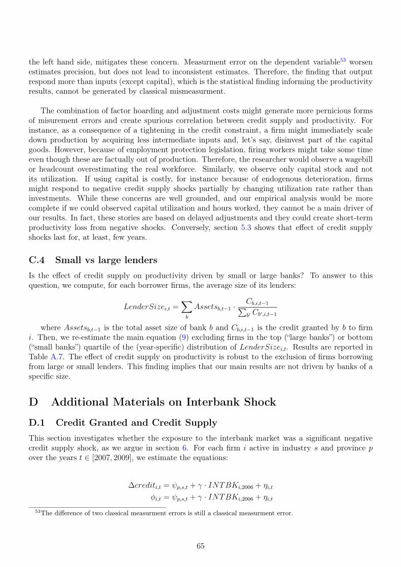
the left hand side, mitigates these concern. Measurment error on the dependent variable53 worsenestimates precision, but does not lead to inconsistent estimates. Therefore, the finding that outputrespond more than inputs (except capital), which is the statistical finding informing the productivityresults, cannot be generated by classical mismeasurment.

The combination of factor hoarding and adjustment costs might generate more pernicious formsof misurement errors and create spurious correlation between credit supply and productivity. Forinstance, as a consequence of a tightening in the credit constraint, a firm might immediately scaledown production by acquiring less intermediate inputs and, let’s say, disinvest part of the capitalgoods. However, because of employment protection legislation, firing workers might take some timeeven though these are factually out of production. Therefore, the researcher would observe a wagebillor headcount overestimating the real workforce. Similarly, we observe only capital stock and notits utilization. If using capital is costly, for instance because of endogenous deterioration, firmsmight respond to negative credit supply shocks partially by changing utilization rate rather thaninvestments. While these concerns are well grounded, and our empirical analysis would be morecomplete if we could observed capital utilization and hours worked, they cannot be a main driver ofour results. In fact, these stories are based on delayed adjustments and they could create short-termproductivity loss from negative shocks. Conversely, section 5.3 shows that effect of credit supplyshocks last for, at least, few years.

C.4 Small vs large lenders

Is the effect of credit supply on productivity driven by small or large banks? To answer to thisquestion, we compute, for each borrower firms, the average size of its lenders:

LenderSizei,t =∑b

Assetsb,t−1 ·Cb,i,t−1∑b′ Cb′,i,t−1

where Assetsb,t−1 is the total asset size of bank b and Cb,i,t−1 is the credit granted by b to firmi. Then, we re-estimate the main equation (9) excluding firms in the top (“large banks”) or bottom(“small banks”) quartile of the (year-specific) distribution of LenderSizei,t. Results are reported inTable A.7. The effect of credit supply on productivity is robust to the exclusion of firms borrowingfrom large or small lenders. This finding implies that our main results are not driven by banks of aspecific size.

D Additional Materials on Interbank Shock

D.1 Credit Granted and Credit Supply

This section investigates whether the exposure to the interbank market was a significant negativecredit supply shock, as we argue in section 6. For each firm i active in industry s and province pover the years t ∈ [2007, 2009], we estimate the equations:

∆crediti,t = ψp,s,t + γ · INTBKi,2006 + ηi,t

φi,t = ψp,s,t + γ · INTBKi,2006 + ηi,t

53The difference of two classical measurment errors is still a classical measurment error.

65

Results are shown in Table A.5, which documents that firms more exposed to the collapse of theinterbank market decrease more the credit received with respect to others operating in the same in-dustry and location. An increase of dependence from the interbank market of 1%, lead to a decreaseof the growth rate of credit granted between a quarter and a fifth of a percentage point, see columns(2) and (4). Furthermore, columns (1) and (3) show that the measure of credit supply shocks φi,tdoes respond negatively to the interbank shocks.

D.2 Interbank and Sensitivity to Business Cycle

A further concern is that, although firms more exposed to interbank market had equal averageproductivity growth before the credit crunch, they were more sensitive to business cycle fluctuationand, therefore, they suffered more during the recession following the financial turmoil. For each firmin the sample, we estimate its sensitivity to business cycle from equation:

∆yi,t = αi + βi ·GDPgrt + εi,t

where GDPgrt is the growth rate of Italian GDP in year t and yi,t is one of two outcomes: (logs)value added or (logs) revenues. The model is estimated using all available years before 2006. Then,we study the correlation between the three measures of sensitivity to fluctuation and the interbankexposure in 2006. Table A.8 shows that firms more exposed to the collapse of the interbank marketwere not significantly more sensitive to downturns before 2006.

D.3 Interbank and Patents

Did the credit crunch affected innovation in Italy? In section 7 we show that credit supply shocks havea significant impact on firm-level innovation. We also provide some descriptive statistics suggestingthat the 2007-08 credit crunch severely damaged patenting activities. Here, we investigate whetherfirms hit harder by the credit crunch patented less afterward. Thus, we estimate the linear model:

PatentGrowthi = ψp + ψs + γINTBKi,2006 + ηi

where

PatentGrowthi = 2 · Patentpost,i − Patentpre,iPatentpost,i + Patentpre,i

and Patentpost,i and Patentpre,i is the total number of patent applications done by firm i in thepost and in the pre periods. The interbank market started collapsing in the late 2007, althoughgeneral economic activity started declining only afterward. We thus use 2007 as the start of the“post” period and 2006 as the end of the “pre” period. We use either 2009 (the very worst yearfor Italian economy) or 2010 (a short period of recovery) as the end of the “post” period. We useeither 2001 or 2002 as start of the “pre” period. Notice that the LHS variable can be computedonly for firms which patent at least once either in the “pre” or “post” period (or both). Results arepresented in Table A.9: firms connected to lenders more exposed to the collapse of the interbankmarket contracted more their patent applications. The boundaries of the periods do not matter.

66

E Additional Materials on Mechanisms

E.1 Notes on R&D and Export

In section 7 we estimate equations:

Pr(R&Di,t = 1) = ψi + ψt + γ · φi,t + ηi,t

Pr(Exporti,t = 1) = ψi + ψt + γ · φi,t + ηi,t

If we include the full set of province×industry×year fixed effects to control for local businesscycle and industry-specific shocks the sample size halves (because of singletons). While the estimatedcoefficients stay in the same ballpark, the standard errors raise enough that we are not able to rejectthe null of no effect on R&D at the conventional level.

67

Additional Figures

.25

.3.3

5.4

.45

1 2 3 4 5Quintile of Assets

Manufacturing Non manufacturing

Credit intensity

Figure A.1: Credit intensity per quintile of asset size. Credit intensity is the ratio of credit granted over netrevenues and it is winsorized at top 2%

0.2

.4.6

.8

0 2 4 6 8Capital/labor ratio

Credit intensity Fitted values

Credit intensity and capital use - industries

0.2

.4.6

.8

0 .5 1 1.5Assets liquidity

Credit intensity Fitted values

Credit intensity and liquidity - industries

Figure A.2: Industry (2-digits) average credit intensity and capital to labor ratio (left panel) or liquidity (rightpanel). Credit intensity is the ratio of credit granted over net revenues and it is winsorized at top 2% before takingaverages. Capital to labor ratio is the ratio of capital stock over total wagebill. Liquidity is the ratio of liquid assetsover book value of capital.

68

0.2

.4.6

.8

0 .2 .4 .6 .8 1Export intensity

Credit Intensity Fitted values

Credit intensity and export - industries

0.2

.4.6

.8

0 .2 .4 .6 .8 1Companies investing in R&D

Credit Intensity Fitted values

Credit intensity and R&D - industries

Figure A.3: Industry (2-digits) average credit intensity and share of companies engaging in export (left panel) orR&D (right panel). Credit intensity is the ratio of credit granted over net revenues and it is winsorized at top 2%before taking averages. Data on export and R&D are taken from INVIND survey (see sections 2 and 7) and representnoisy estimate of the effective export and R&D intensity. The the slope of the fitted line in left panel is significantlylarger from zero, while the one in the right panel is statistically indistinguishable from zero.

-.008

-.006

-.004

-.002

1 2 3 4 5Quintile of credit supply shock

CD - Revenue Prod TL - Revenue Prod

Mean productivity growth

Figure A.4: Average productivity growth per quintile of credit supply shock

-.1-.0

50

.05

-.6 -.4 -.2 0 .2Productivity growth

Credit supply shock Fitted values

Cobb - Douglas

-.1-.0

50

.05

-.6 -.4 -.2 0 .2 .4Productivity growth

Credit supply shock Fitted values

Trans Log

Figure A.5: Industry×year average revenue productivity growth and credit supply shocks. Fitted lines in bothpanels have a slop significantly larger than zero (1% confidence). We drop two observations with extremely negativevalue of average the credit supply shock

69

-.15

-.1

-.05

0.0

5.1

Shi

fter

1995 2000 2005 2010 2015year

-.1

-.05

0.0

5.1

Shi

fter

1995 2000 2005 2010 2015year

Figure A.6: Figures display evolution of Credit Supply Shock experienced by a 1.5% random sample. Right panelshows residualized values after taking out FEs

-4-2

02

4P

rodu

ctiv

ity R

esid

ual

1995 2000 2005 2010 2015year

-2-1

01

2P

rodu

ctiv

ity G

row

th

1995 2000 2005 2010 2015year

Figure A.7: Figures display evolution of Productivity (Cobb-Douglas, Value Added) for 1.5% random sample.Right panel shows residualized values after taking out FEs

70

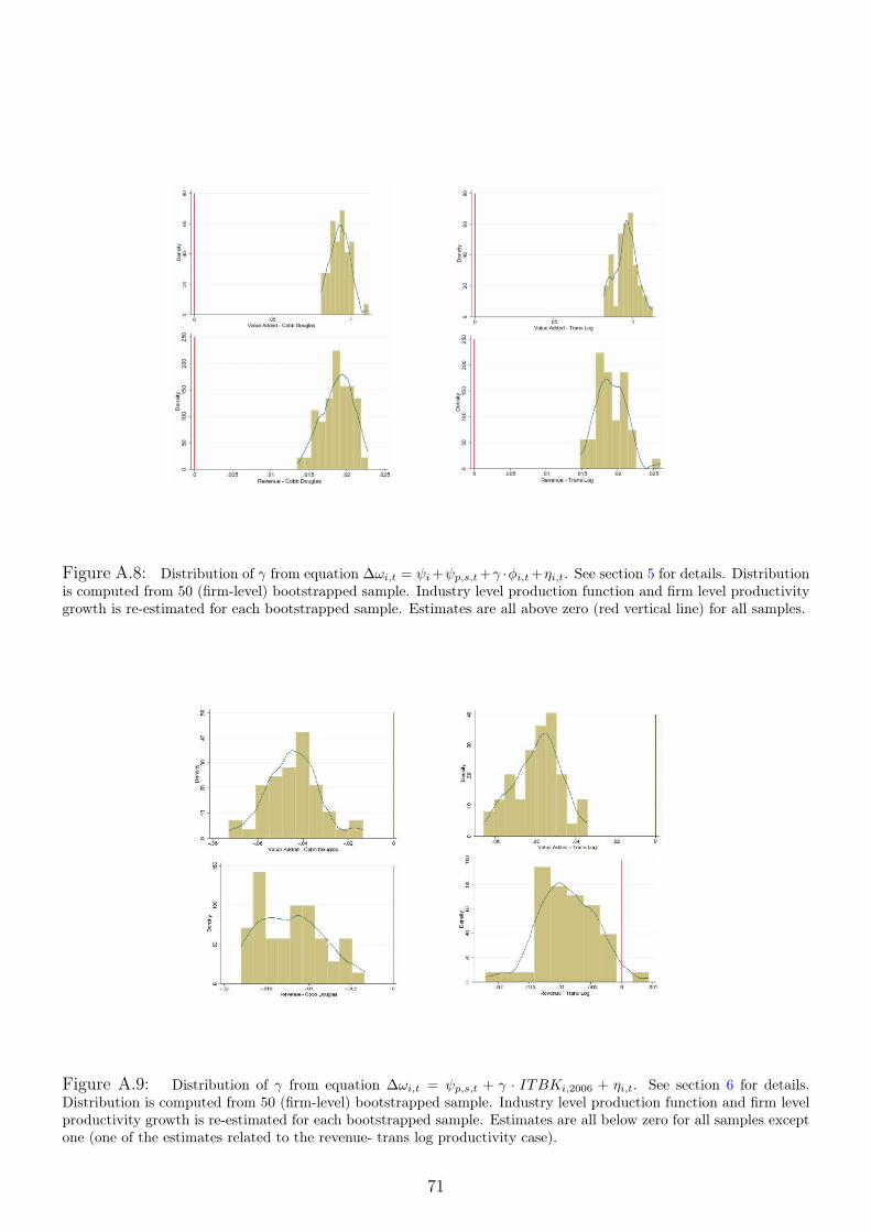
Figure A.8: Distribution of γ from equation ∆ωi,t = ψi+ψp,s,t+γ ·φi,t+ηi,t. See section 5 for details. Distributionis computed from 50 (firm-level) bootstrapped sample. Industry level production function and firm level productivitygrowth is re-estimated for each bootstrapped sample. Estimates are all above zero (red vertical line) for all samples.

Figure A.9: Distribution of γ from equation ∆ωi,t = ψp,s,t + γ · ITBKi,2006 + ηi,t. See section 6 for details.Distribution is computed from 50 (firm-level) bootstrapped sample. Industry level production function and firm levelproductivity growth is re-estimated for each bootstrapped sample. Estimates are all below zero for all samples exceptone (one of the estimates related to the revenue- trans log productivity case).

71

Additional Tables

Table A.1: Credit Supply Shock and Loan Applications to New Lenders

VARIABLES N. of PI N. of PI | N>0 Pr(N. of PI >0)(1) (2) (3)

All Industries

φi,t -0.537*** -0.458*** -0.0780***(0.0796) (0.113) (0.0173)

Observations 656,960 456,888 656,960R2 0.500 0.477 0.348

Manufacturing

φi,t -0.424*** -0.355** -0.0583**(0.113) (0.161) (0.0242)

Observations 347,990 246,453 347,990R2 0.491 0.462 0.349

Notes: One observation is one firm for one year between 1998 and 2013 (unbalanced panel).Firm FEs and province×industry×year FEs are included. Singleton are dropped. TheRHS variable φi,t represents idiosyncratic shock to firm credit supply, and its construction isdetailed in section 3.1. A 1% increase in φi,t is the supply shock needed to increase the creditgranted to firm i by 1%. The LHS variables are built from the number of banks which requestinformation about firm i in year t and they proxy for the number of of firm i’ applications withpreviously unconnected lenders. Column (1) conflates both intensive and extensive margin,while (2) is a linear probability model for the probability of making any application. Column(3) considers the extensive margin only. Standard errors (in parentheses) are clustered atfirm level. *** p<0.01, ** p<0.05, * p<0.1

72

Table A.2: Descriptive Statistics - Cobb Douglas Parameters

VARIABLE Mean Std. Dev. Mean Std. Dev.(Quantity) (Quantity)

All IndustriesValue Added

βl .64 .16 .85 .25βk .17 .14 .22 .19

Revenuesβl .14 .17 .18 .22βk .06 .06 .08 .08βm .81 .11 1.08 .25

ManufacturingValue Added

βl .62 .15 .81 .22βk .19 .16 .24 .21

Revenuesβl .13 .05 .17 .07βk .04 .02 .05 .03βm .81 .1 1.06 .12

Notes: βx is the estimated elasticity of output with respect to input x. Estimationof the parameters is performed at sector level, details are provided in section 3.2.Standard deviation represent sectoral variations and not estimation error. “Quan-tity” parameters are calculated by multiplying the estimate of sales-generating pro-duction function by the correction term σ

σ−1 , where σ is the elasticity of demand.The correction is exact if firms are monopolistic competitors, see De Loecker (2011).σ is estimated from self-reported elasticity of demand, as in Pozzi & Schivardi(2016).

Table A.3: Credit Supply Shock and Productivity Growth (alternative model)

VARIABLES Productivity Productivity Productivity Productivity(in delta Log)

(1) (2) (3) (4)

φi,t 0.117*** 0.0347*** 0.100*** 0.0231***(0.0178) (0.00589) (0.0145) (0.00412)

Observations 347,990 347,990 656,960 656,960R2 0.194 0.146 0.182 0.172

Functional Form Cobb-Douglas Cobb-Douglas Cobb-Douglas Cobb-DouglasOutput Measure Value Added Net Revenues Value Added Net Revenues

Sample Manufacturing Manufacturing All AllNotes: One observation is one firm for one year (panel). Firm FEs andprovince×industry×year FEs are included. The RHS variable φi,t represents idiosyncraticshock to firm credit supply, and its construction is detailed in section A.1. Productivity isestimated following the model in section B.2. Standard errors (in parentheses) are clusteredat firm level. *** p<0.01, ** p<0.05, * p<0.1

73

Table A.4: Credit Supply Shock and Productivity Growth - Heterogeneity by Demand Elasticity

VARIABLES Productivity Productivity Productivity Productivity(in delta Log)

(1) (2) (3) (4)All Industries

φi,t 0.0854*** 0.101*** 0.0146*** 0.0199***(0.0169) (0.0175) (0.00445) (0.00470)

φi,t ·HSs 0.0399 0.0345 0.0156 0.0221*(0.0321) (0.0342) (0.0134) (0.0121)

Observations 649,662 649,662 649,662 649,662R-squared 0.170 0.182 0.176 0.188

Manufacturing

φi,t 0.0774*** 0.0906*** 0.0201** 0.0171*(0.0255) (0.0260) (0.00823) (0.00938)

φi,t ·HSs 0.0787** 0.0623* 0.0212* 0.0316**(0.0354) (0.0374) (0.0121) (0.0132)

Observations 347,990 347,990 347,990 347,990R-squared 0.186 0.200 0.144 0.180

Notes: ∆ωi,t = ψi+ψs,t,p+(γ + γσ ·HEs)·φi,t+ηi,t. One observation is one firm for one yearbetween 1998 and 2013 (unbalanced panel). Firm FEs and province×industry×year FEs areincluded. Singleton are dropped. The RHS variable φi,t represents idiosyncratic shock tofirm credit supply, and its construction is detailed in section 3.1. A 1% increase in φi,t isthe supply shock needed to increase the credit granted to firm i by 1%. The LHS variable isthe first difference of Hicks-neutral productivity residual: ∆ωi,t = ∆yi,t −∆f(xi,t, β) wherey is log of net revenues (or log of value added) and x is a set of inputs. Capital stock, labor,and (for the revenue case only) intermediate inputs are included in x. f(·, β) is either afirst (Cobb-Douglas) or second (Trans-Log) order polynomial in log inputs. Estimation ofparameters β is described in section 3.2. HEs is a dummy variable equal to one iff firm iis in an industry with elasticity of demand above the sample median. Sectoral elasticitiesare calculated from INVIND (1996 and 2007 waves) self-reported elasticity of demand (wetake median of all responses within a 2-digits industry). Standard errors (in parentheses)are clustered at firm level. *** p<0.01, ** p<0.05, * p<0.1

74

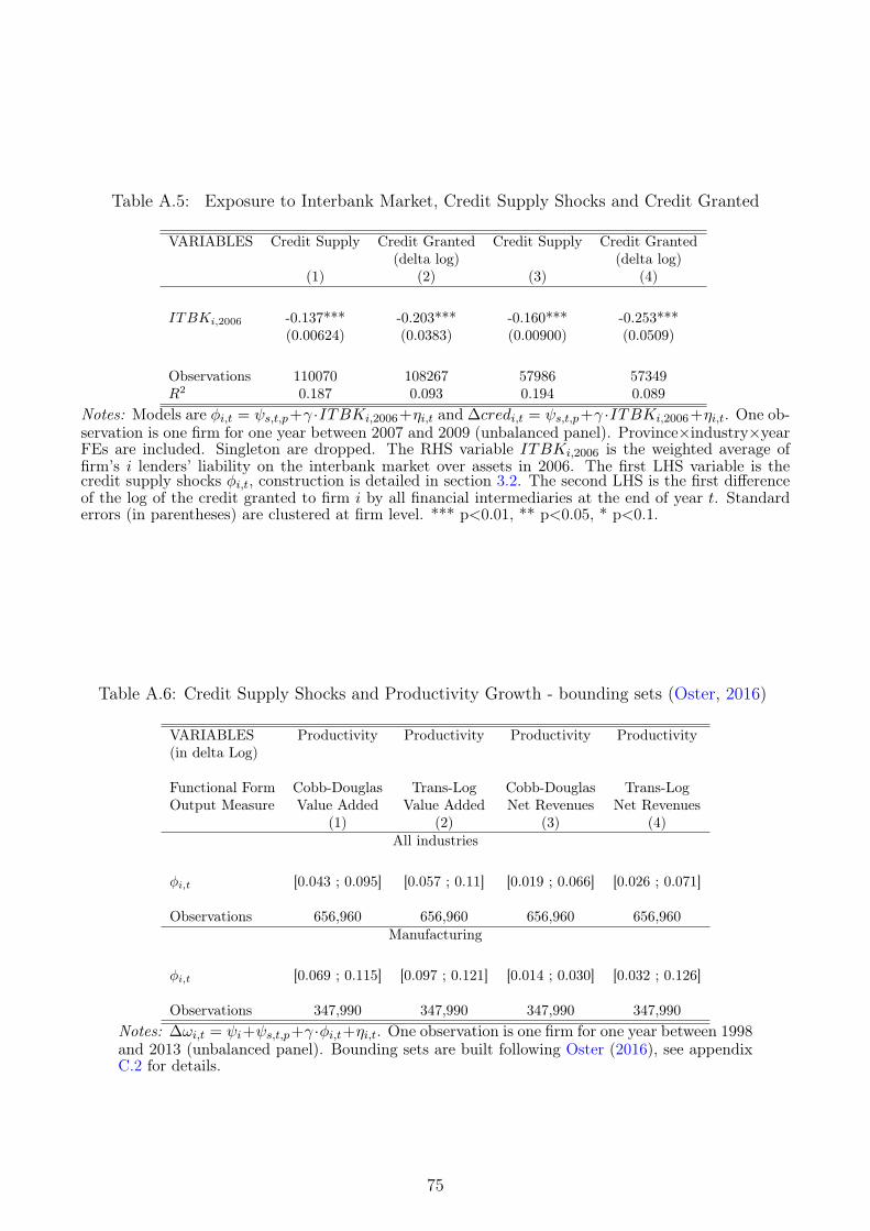
Table A.5: Exposure to Interbank Market, Credit Supply Shocks and Credit Granted

VARIABLES Credit Supply Credit Granted Credit Supply Credit Granted(delta log) (delta log)

(1) (2) (3) (4)

ITBKi,2006 -0.137*** -0.203*** -0.160*** -0.253***(0.00624) (0.0383) (0.00900) (0.0509)

Observations 110070 108267 57986 57349R2 0.187 0.093 0.194 0.089

Notes: Models are φi,t = ψs,t,p+γ ·ITBKi,2006+ηi,t and ∆credi,t = ψs,t,p+γ ·ITBKi,2006+ηi,t. One ob-servation is one firm for one year between 2007 and 2009 (unbalanced panel). Province×industry×yearFEs are included. Singleton are dropped. The RHS variable ITBKi,2006 is the weighted average offirm’s i lenders’ liability on the interbank market over assets in 2006. The first LHS variable is thecredit supply shocks φi,t, construction is detailed in section 3.2. The second LHS is the first differenceof the log of the credit granted to firm i by all financial intermediaries at the end of year t. Standarderrors (in parentheses) are clustered at firm level. *** p<0.01, ** p<0.05, * p<0.1.

Table A.6: Credit Supply Shocks and Productivity Growth - bounding sets (Oster, 2016)

VARIABLES Productivity Productivity Productivity Productivity(in delta Log)

Functional Form Cobb-Douglas Trans-Log Cobb-Douglas Trans-LogOutput Measure Value Added Value Added Net Revenues Net Revenues

(1) (2) (3) (4)All industries

φi,t [0.043 ; 0.095] [0.057 ; 0.11] [0.019 ; 0.066] [0.026 ; 0.071]

Observations 656,960 656,960 656,960 656,960Manufacturing

φi,t [0.069 ; 0.115] [0.097 ; 0.121] [0.014 ; 0.030] [0.032 ; 0.126]

Observations 347,990 347,990 347,990 347,990Notes: ∆ωi,t = ψi+ψs,t,p+γ ·φi,t+ηi,t. One observation is one firm for one year between 1998and 2013 (unbalanced panel). Bounding sets are built following Oster (2016), see appendixC.2 for details.

75

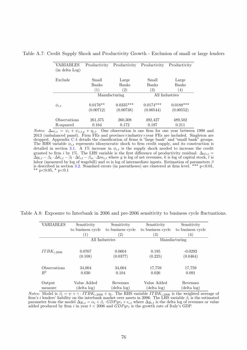
Table A.7: Credit Supply Shock and Productivity Growth - Exclusion of small or large lenders

VARIABLES Productivity Productivity Productivity Productivity(in delta Log)

Exclude Small Large Small LargeBanks Banks Banks Banks(1) (2) (3) (4)Manufacturing All Industries

φi,t 0.0176** 0.0335*** 0.0174*** 0.0188***(0.00712) (0.00738) (0.00544) (0.00552)

Observations 261,375 260,308 492,427 489,502R-squared 0.164 0.172 0.197 0.211

Notes: ∆ωi,t = ψi + ψs,t,p + ηi,t. One observation is one firm for one year between 1998 and2013 (unbalanced panel). Firm FEs and province×industry×year FEs are included. Singleton aredropped. Appendix C.4 details the classification of firms is “large bank” and “small bank” groups.The RHS variable φi,t represents idiosyncratic shock to firm credit supply, and its construction isdetailed in section 3.1. A 1% increase in φi,t is the supply shock needed to increase the creditgranted to firm i by 1%. The LHS variable is the first difference of productivity residual: ∆ωi,t =∆yi,t − βk ·∆ki,t − βl ·∆li,t − βm ·∆mi,t where y is log of net revenues, k is log of capital stock, l islabor (measured by log of wagebill) and m is log of intermediate inputs. Estimation of parameters βis described in section 3.2. Standard errors (in parentheses) are clustered at firm level. *** p<0.01,** p<0.05, * p<0.1

Table A.8: Exposure to Interbank in 2006 and pre-2006 sensitivity to business cycle fluctuations.

VARIABLES Sensitivity Sensitivity Sensitivity Sensitivityto business cycle to business cycle to business cycle to business cycle

(1) (2) (3) (4)All Industries Manufacturing

ITBKi,2006 0.0767 0.0604 0.195 -0.0292(0.108) (0.0377) (0.225) (0.0464)

Observations 34,004 34,004 17,759 17,759R2 0.030 0.104 0.026 0.091

Output Value Added Revenues Value Added Revenuesmeasure (delta log) (delta log) (delta log) (delta log)

Notes: Model is βi = ψ + γ · ITBKi,2006 + ηi. The RHS variable ITBKi,2006 is the weighted average offirm’s i lenders’ liability on the interbank market over assets in 2006. The LHS variable βi is the estimatedparameter from the model ∆yi,t = αi + βi ·GDPgrt + εi,t where ∆yi,t is the delta log of revenues or valueadded produced by firm i in year t < 2006 and GDPgrt is the growth rate of Italy’s GDP.

76

Table A.9: Exposure to Interbank in 2006 and growth of patent applications

VARIABLES Patent Patent PatentGrowth Growth Growth

“Pre” [2003;2006] [2002;2006] [2002;2006]“Post” [2007;2009] [2007;2010] [2007;2009]

(1) (2) (3)

-1.463* -1.703** -1.738**(0.783) (0.834) (0.747)

Observations 2,903 3,217 3,040R-squared 0.058 0.054 0.057

Notes: Results of estimating model:

PatentGrowthi = ψp + ψs + γINTBKi,2006 + ηi

where PatentGrowthi = 2 · Patentpost,i−Patentpre,iPatentpost,i+Patentpre,i. Patentpost,i

(Patentpre,i) is the total number of patent applications made by firmi in the “pre” (“post”) period. The three columns are different becauseof the definition of “pre” and “post” periods.

Table A.10: Bank characteristics, M&A and credit supply shocks

VARIABLES Credit Supply Credit Supply Credit Supply Credit supply(delta log)Years [2007,2009] [2007,2009] [2010,2013] All years

Unit of Bank Bank Bank Firmobservation

(1) (2) (3) (4)(loansdeposits

)b,2007

-0.0189***

(0.00533)(capitalRWA

)b,2007

0.00133**

(0.000588)∆(sovereignAssets

)b,t

-0.155***(0.0400)

M&Ai,t -0.0117***(0.000657)

Observations 1,635 1,635 2,034 652,692R-squared 0.086 0.076 0.010 0.521

Notes: Columns (1)-(2): model is φb,t = ψt + γ · Xb,τ + ηb,t where φb,t is abank-level measure of changes in credit supply (see section 3.1 for details) andXb,2007 is a bank-level characteristic at time 2007. Column (3): model is φb,t =

ψt + γ ·∆(sovereignAssets

)b,t

+ ηb,t where(sovereignAssets

)b,t

is the share of sovereign debt

on bank b assets. Column (4): model is φi,t = ψi + ψp,s,t + γ ·MAi,t + ηi,t whereφi,t is a firm-level measure of shock to credit supply (see section 3.1 for details)and MAi,t is the share of firm i previous period lenders which undergo a mergerand acquisition (as a target).

77

TableA.11:

CreditSu

pply

Shocks

andProdu

ctivity

Growth:Rob

ustness-Cob

b-Dou

glas

Value

Add

edProdu

ctivity

VARIA

BLE

SProdu

ctivity

Produ

ctivity

Produ

ctivity

Produ

ctivity

Produ

ctivity

Produ

ctivity

Produ

ctivity

Produ

ctivity

Produ

ctivity

(delta

Logs)

Mod

elBaseline

Firm

Impo

rtan

tPoo

led

Alterna

tive

Match

Split

4Digits

End

ogenou

sCon

trols

Borrowers

Estim

ator

FEsstructure

Con

trols

Sample

Sector

Exit

(1)

(2)

(3)

(4)

(5)

(6)

(7)

(8)

(9)

AllIndu

stries

φi,t

0.0946***

0.106***

0.0865***

0.0436***

0.0968***

0.101***

0.0932***

0.0988***

0.0898***

(0.0155)

(0.0175)

(0.0172)

(0.00963)

(0.0151)

(0.0188)

(0.0164)

(0.0183)

(0.0156)

Observation

s656,960

483,665

521,741

656,960

656,960

656,960

656,960

587,873

656,960

R-squ

ared

0.172

0.191

0.185

0.021

0.104

0.172

0.172

0.267

0.175

Man

ufacturing

φi,t

0.115***

0.122***

0.126***

0.0405***

0.116***

0.114***

0.114***

0.127***

0.111***

(0.0178)

(0.0211)

(0.0196)

(0.0120)

(0.0180)

(0.0216)

(0.0188)

(0.0208)

(0.0180)

Observation

s347,990

262,308

280,346

347,990

347,990

347,990

347,990

309,887

347,990

R-squ

ared

0.186

0.209

0.198

0.032

0.110

0.186

0.186

0.278

0.191

Not

es:Mod

elis

∆ωi,t

=ψi+ψs,t,p

+γ·φ

i,t+η i,tOne

observationison

efirm

foron

eyear

betw

een1998

and2013

(unb

alan

cedpa

nel).Firm

FEsan

dprovince×indu

stry×year

FEsareinclud

ed.Sing

letonaredrop

ped.

The

RHSvariab

leφi,trepresents

idiosync

raticshockto

firm

cred

itsupp

ly,a

nditsconstruc

tion

isde

taile

din

section3.1.

A1%

increase

inφi,tis

thesupp

lyshockne

eded

toincrease

thecred

itgran

ted

tofirmiby

1%.The

LHSvariab

leis

thefirst

diffe

renc

eof

prod

uctivity

residu

al:

∆ωi,t

=∆vai,t−βk·∆

ki,t−βl·∆

l i,twhe

revais

logof

netvaluead

ded,kislogof

capitalstock

andlislabo

r(m

easuredby

logof

wag

ebill).

Estim

ationof

parametersβisde

scribe

din

section3.2.

Colum

n(2)ad

dasetof

lagg

edcontrolsto

baselin

especification

:po

lyno

mialinsize

(assets)

andtheratios

ofvaluead

ded,

liquidity,c

ashflo

wan

dba

nkde

btto

assets.It

exclud

esob

servationwithmissing

orzero

values

foran

ycontrolv

ariable.

Colum

n(3)exclud

esan

yfirm

that,a

tan

ypo

intin

time,

received

morethan

1%of

thecred

itby

anyfin

ancial

interm

ediary.Colum

n(4)usepo

oled

estimator

(rathe

rthan

“within”)

bydrop

ping

firm

FEs.

Colum

n(5)includ

esfirm

FEs,province

FEs,year

FEsan

dindu

stry

FEs,bu

tdo

notinclud

eprov

ince×year×indu

stry

FEs.

Colum

n(6)uses

analternativemeasure

ofcred

itsupp

lyshocks

which

controlfor

match-spe

cific

covariates,see

section3.1.

Colum

n(7)

uses,as

aninstrument,

analternativecred

itsupp

lyshocks

estimated

witha“split

sample”

proced

ure,

inorde

rto

controlforfin

itesample

biases.Colum

n(8)uses

a4-digits

(rathe

rthan

2)indu

stry

defin

itionbo

thfortheestimationof

prod

uctivity

parametersan

dfortheFEs

structure.

Itcontains

less

observations

becauseof

thesing

letondrop

ping

.Colum

n(9)estimateprod

uctivity

allowingforen

dogeno

usfirm

exit,a

sin

Olle

y&

Pak

es(199

6).Stan

dard

errors,inpa

renthe

ses,are(two-way

)clusteredat

firm

andmain-ba

nk×year

level.***p<

0.01,*

*p<

0.05

,*p<

0.1

78

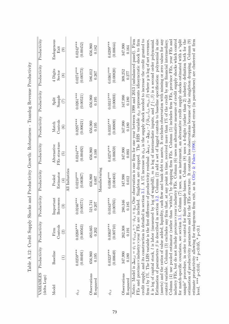
TableA.12:

CreditSu

pply

Shocks

andProdu

ctivity

Growth:Rob

ustness-Tr

anslog

Revenue

Produ

ctivity

VARIA

BLE

SProdu

ctivity

Produ

ctivity

Produ

ctivity

Produ

ctivity

Produ

ctivity

Produ

ctivity

Produ

ctivity

Produ

ctivity

Produ

ctivity

(delta

Logs)

Mod

elBaseline

Firm

Impo

rtan

tPoo

led

Alterna

tive

Match

Split

4Digits

End

ogenou

sCon

trols

Borrowers

Estim

ator

FEsstructure

Con

trols

Sample

Sector

Exit

(1)

(2)

(3)

(4)

(5)

(6)

(7)

(8)

(9)

AllIndu

stries

φi,t

0.0259***

0.0268***

0.0246***

0.0210***

0.0244***

0.0297***

0.0261***

0.0274***

0.0242***

(0.00491)

(0.00563)

(0.00571)

(0.00367)

(0.00492)

(0.00621)

(0.00521)

(0.00573)

(0.00452)

Observation

s656,960

483,665

521,741

656,960

656,960

656,960

656,960

586,012

656,960

R-squ

ared

0.195

0.202

0.207

0.007

0.100

0.195

0.195

0.267

0.182

Man

ufacturing

φi,t

0.0323***

0.0363***

0.0343***

0.0304***

0.0274***

0.0335***

0.0315***

0.0361***

0.0299***

(0.00649)

(0.00710)

(0.00765)

(0.00483)

(0.00659)

(0.00809)

(0.00693)

(0.00820)

(0.00644)

Observation

s347,990

262,308

280,346

347,990

347,990

347,990

347,990

309,252

347,990

R-squ

ared

0.180

0.191

0.185

0.012

0.093

0.180

0.180

0.277

0.164

Not

es:Mod

elis

∆ωi,t

=ψi+ψs,t,p

+γ·φ

i,t+η i,tOne

observationison

efirm

foron

eyear

betw

een1998

and2013

(unb

alan

cedpa

nel).Firm

FEsan

dprovince×indu

stry×year

FEsareinclud

ed.Sing

letonaredrop

ped.

The

RHSvariab

leφi,trepresents

idiosync

raticshockto

firm

cred

itsupp

ly,a

nditsconstruc

tion

isde

taile

din

section3.1.

A1%

increase

inφi,tisthesupp

lyshockne

eded

toincrease

thecred

itgran

tedto

firmiby

1%.The

LHSvariab

leisthefirst

diffe

renc

eof

prod

uctivity

residu

al:

∆ωi,t

=∆y i,t−f

(ki,t,l i,t,m

i,t,β

)whe

reyislogof

netrevenu

es,

kis

logof

capitalstock,lis

labo

r(m

easuredby

logof

wag

ebill),m

islogof

interm

ediate

inpu

ts,an

df

(·,β

)is

asecond

orde

rpo

lyno

mial.

Estim

ationof

parametersβis

describe

din

section3.2.

Colum

n(2)ad

dasetof

lagg

edcontrols

toba

selin

especification

:po

lyno

mialinsize

(assets)

andtheratios

ofvaluead

ded,

liquidity,c

ashflo

wan

dba

nkde

btto

assets.It

exclud

esob

servationwithmissing

orzero

values

foran

ycontrolv

ariable.

Colum

n(3)exclud

esan

yfirm

that,a

tan

ypo

intin

time,

received

morethan

1%of

thecred

itby

anyfin

ancial

interm

ediary.

Colum

n(4)usepo

oled

estimator

(rathe

rthan

“within”)by

drop

ping

firm

FEs.

Colum

n(5)includ

esfirm

FEs,

province

FEs,

year

FEsan

dindu

stry

FEs,bu

tdo

notinclud

eprov

ince×year×indu

stry

FEs.

Colum

n(6)uses

analternativemeasure

ofcred

itsupp

lyshocks

which

control

formatch-spe

cific

covariates,s

eesection3.1.

Colum

n(7)uses,a

san

instrument,

analternativecred

itsupp

lyshocks

estimated

witha“split

sample”

proced

ure,

inorde

rto

controlforfin

itesamplebiases.Colum

n(8)uses

a4-digits

(rathe

rthan

2)indu

stry

defin

itionbo

thforthe

estimationof

prod

uctivity

parametersan

dfortheFEsstructure.

Itcontains

less

observations

becauseof

thesing

letondrop

ping

.Colum

n(9)

estimateprod

uctivity

allowingforen

dogeno

usfirm

exit,as

inOlle

y&

Pakes

(199

6).Stan

dard

errors

(inpa

renthe

ses)

areclusteredat

firm

level.

***p<

0.01

,**p<

0.05

,*p<

0.1

79