13 December 2017 Trust in water Delivering Water … · Appendix to Chapter 10: Aligning risk and...

13 December 2017 Trust in water

Delivering Water 2020:

Our methodology for the

2019 price review

Appendix 12: Aligning risk

and return

Appendix to Chapter 10: Aligning risk and return

www.ofwat.gov.uk

Delivering Water 2020: Our methodology for the 2019 price review Appendix 12: Aligning risk and return

1

Contents

1. Summary ............................................................................................................. 2

2. Overall balance of risk and return ........................................................................ 4

3. Scenario analysis and risk assessment ............................................................. 10

4. Our early view on the cost of capital .................................................................. 16

5. Our approach to the cost of equity ..................................................................... 23

6. Our approach to the cost of debt ....................................................................... 69

7. Company-specific adjustments to the cost of capital ......................................... 85

8. Our decision to index price controls to CPIH ..................................................... 95

9. Taxation ........................................................................................................... 101

10. The impact of an altered mix of real and nominal returns on cash flow ratios ....

..................................................................................................................... 109


2

1. Summary

This appendix sets out further detail of our final methodology for our 2019 price

review (PR19) with respect to aligning risk and return across the price controls. This

methodology has been determined following full consideration of the views

expressed by respondents to our draft methodology proposals, published in July of

this year.

This appendix supplements the information on aligning risk and return, set out in

chapters 10 (aligning risk and return) and 11 (aligning risk and return: financeability)

of our PR19 final methodology.

Our aim is to align the interests of companies and investors with those of customers,

by setting the appropriate balance of risk and return. This means that by responding

to our incentives in the way that is best for them, companies will also deliver what is

best for customers.

Applicability to England and Wales

Our PR19 final methodology for risk and return applies to both companies whose areas

are wholly or mainly in England, and companies whose areas are wholly or mainly in

Wales.

Our approach to setting a retail net margin reflects the different circumstances in England and Wales.

Eligible business customers of companies whose areas are wholly or mainly in England are able to choose

their supplier; in most cases, appointed companies have exited the market and so they do not have a

business retail operation that could be subject to a price control. Where appointees have not exited the

market, we will set a price control. As discussed in chapter 10, we will continue to set retail controls for

business customers in Wales.

We discuss our decisions for the overall balance of risk and return, and set out our

expectations for scenario analysis in the business plans. We also set out the

responses we have received in respect of our draft methodology proposals, and how

we will assess the evidence to inform our early view on the cost of capital. We

provide further details on the assessment we will undertake for claims for company

specific adjustments to the cost of capital and set out our decisions on our choice of

inflation index and our approach to tax.

http://www.ofwat.gov.uk/consultation/delivering-water2020-consulting-on-our-methodology-for-the-2019-price-review/


3

Section 9 of Appendix 15 outlines respondents’ views to the questions we posed on

risk and return in our draft methodology consultation. In Appendix 15, we provide (or

reference) our response to the issues raised by respondents.

https://www.ofwat.gov.uk/publication/delivering-water-2020-final-methodology-2019-price-review-appendix-15-responses-draft-methodology/https:/www.ofwat.gov.uk/publication/delivering-water-2020-final-methodology-2019-price-review-appendix-15-responses-draft-methodology/


4

2. Overall balance of risk and return

2.1 Our proposed position as set out in the draft methodology

In our draft methodology proposals, we said that price controls are most effective

where the interests of investors and companies are aligned with those of customers,

in both the short and the long term.

To achieve this alignment, we explained that the regime currently embeds a number

of incentives designed to mimic competitive pressures. This is aimed at driving better

business planning and incentivising company management to deliver better service

at an efficient cost.

In our draft methodology proposals, we said that evidence from PR14 and the

current price control period suggests reputational and procedural incentives are

effective. We also made clear in our draft methodology proposals, that where we

need to further sharpen incentives, we can do so with well calibrated financial

incentives. These align companies’ interests with those of their customers.

Our draft methodology proposals were as follows:

for outcomes, we stated that we expect that our proposed measures will mean

an average company with average performance would expect to incur

underperformance penalties on its ODI package, rather than outperformance

payments. We proposed to remove the RoRE cap of ±2% and give an

indicative, uncapped, range of ±1-3%;

we proposed to remove menu regulation and replace it with a cost sharing

scheme that incentivises companies to submit stretching cost forecasts; and

we proposed that companies with exceptional business plans would get a

20bp RoRE incentive payment. We proposed to set a lower cost sharing rate

for companies assessed as requiring significant scrutiny.

We did not ask any specific consultation questions on the balance of risk and return

in our draft methodology proposals. However, respondents raised a number of

issues relating to the balance of risk and return that we address in this document.

2.2 Responses to our draft methodology proposals

Respondents raised the following issues with regard to the balance of risk and

return:


5

most respondents that commented raised concerns that the overall balance of

risk and return was skewed to the downside;

some respondents considered that the downside skew and the use of upper

quartile benchmarks meant that the majority of companies would not earn

their allowed cost of capital – some respondents considered that this would be

true even for well performing companies;

some respondents considered that the wider range of potential

outperformance and underperformance adjustments required a higher cost of

equity;

some respondents considered that to perform well on outcomes, companies

must spend more on totex; and

some respondents considered that excluding glide-paths would increase the

efficiency challenge.

2.3 Our final position

Elements of the balance of risk and return

Our final decision on outcomes, cost sharing rates and incentive payments under the

initial assessment of business plans (IAP) are discussed in chapter 4 (outcomes),

chapter 9 (cost efficiency) and chapter 14 (initial assessment of business plans)

respectively.

Balance of risk and return

We have considered carefully the views of respondents to our draft methodology

proposals. We do not consider our approach skews potential returns to the

downside. Our aim is to incentivise companies to be ambitious, and in so doing,

deliver more of what matters for customers. Companies are able to manage

downside risk by ensuring they deliver for customers.

A company with average current performance that maintains the same absolute level

of performance into the next price control period would incur underperformance

penalties on its ODIs. This is because we are expecting companies to improve and

are setting challenges for performance commitments, including a forward-looking,

upper-quartile challenge. This led some respondents to raise concerns that the

overall balance of risk at PR19 would therefore be skewed to the downside. We do

not believe that this is the case; we are simply expecting companies to improve,

consistent with improvements in previous periods and the wider economy. Average,

or even efficient, performance now will not equate to efficient performance in the

future. It will be possible, if unlikely, for all companies to outperform their


6

performance commitments and earn net ODI outperformance payments in the next

price control period.

There is evidence that once price determinations have been set, company

management focuses on the most challenging areas of the price control, to mitigate

downside risk. For example, the simple average of companies’ PR14 RoRE scenario

P10 P90 ranges1 for ODI impacts implied that companies expected RoRE impact of

-0.6%2 across the sector. Outturn data to date3 shows the actual outcome has been

a +0.1% RoRE impact. Therefore, outturn returns can be skewed to the upside – due

to the effect of information asymmetry and management actions to deliver improved

levels of performance. This evidence supports our view that efficient companies

should expect to earn the allowed returns.

Impact of range of returns on required expected returns

By proposing a wider range for the RoRE impact of ODIs, and by increasing the

exposure of companies to the impact of management decisions, for example,

through the form of the bioresources price control, we have increased the overall

distribution of possible outturn returns. Some respondents considered that this

should be reflected in a higher cost of capital. We disagree. Our reasoning for

broadening the range of expected returns is to align the interests of companies and

their investors with customers. It is also to encourage investors to take more interest

in the actual performance of the companies. The wider range of potential outturn

returns is a diversifiable risk and not, therefore, a factor which leads investors to

require a higher return.

Achieving low costs and excellent service

Some respondents argued that it is difficult to achieve strong performance on costs

and outcomes at the same time, because in order to achieve better outcomes,

companies could need to increase totex spend. However, sector evidence shows

1 P10 P90 ranges are discussed further in section 3.1 below. 2 PwC analysis ’Refining the balance of incentives for PR19’, June 2017 3 Based on average performance over 2015-16 and 2016-17 as reported in Ofwat 2017 Monitoring Financial Resilience. Note that this is indicative only as performance on some ODIs will not be known until the end of the period.

https://064f1d25f5a6fb0868ac-0df48efcb31bcf2ed0366d316cab9ab8.ssl.cf3.rackcdn.com/wp-content/uploads/2017/07/PwC-Balance-of-incentives-June2017.pdf

https://064f1d25f5a6fb0868ac-0df48efcb31bcf2ed0366d316cab9ab8.ssl.cf3.rackcdn.com/wp-content/uploads/2017/11/Monitoring-financial-resilience-report-2017-Final.pdf

https://064f1d25f5a6fb0868ac-0df48efcb31bcf2ed0366d316cab9ab8.ssl.cf3.rackcdn.com/wp-content/uploads/2017/11/Monitoring-financial-resilience-report-2017-Final.pdf


7

that, if anything, the opposite is true. There is evidence that low cost companies also

perform well on service. Our analysis supports the view that companies can perform

well across a range of regulatory metrics concurrently, which may be a feature of

good management.

This relationship is shown best by assessing performance under the service

incentive mechanism (SIM) against retail costs. Figure 1, compares 2015-16 and

2016-17 SIM scores to retail opex performance (which excludes the impact of capital

costs), where we find a correlation of 0.68 across 2015-16 and 2016-174. PwC drew

similar conclusions in its analysis of SIM and retail data for 2011-145.

While correlations between ODI and cost data are not as strong, we have observed

that there is a positive relationship between the more cost efficient companies which

also report better outcome performance, as shown in Figure 2.

Figure 1: Retail opex performance and SIM performance for 2015-16 and 2016-17

4 Ofwat analysis. 5 See section 4 of PwC 2017 Refining the balance of incentives for PR19

70

75

80

85

90

95

-20% -10% 0% 10% 20%

SIM

sc

ore

Retail opex performance

Underperform (overspend) Outperform (underspend)



8

Figure 2: Totex, including retail costs, and ODI performance for 2015-16 and 2016-17

Glide-paths

We will set our benchmarks on the basis of comparative assessment for costs and

service levels. Glide-paths may be appropriate where we make use of a new

benchmark, or companies have not had prior knowledge of the likely scale of the

challenge. Glide-paths can be applied to performance commitments on service

levels, or to efficiency challenges on costs. This was the case for the residential retail

cost challenge and comparative ODIs at PR14, where we applied a glide-path.

For costs, we do not consider that glide-paths that take inefficient companies to

efficient levels are appropriate where we have previously set cost challenges, and so

companies are well placed to be able to judge their likely relative efficiency. Including

a glide-path would result in customers paying for inefficient costs for longer. For

PR19, we therefore will not be using glide-paths for network plus totex and

residential retail costs, as cost assessment for these areas has been subject to

benchmark setting through previous price controls. However, glide-paths may be

appropriate for bioresources and water resources, if the separate cost assessment

for them significantly shift the cost frontier forward for PR19. We will take a

-20

-15

-10

-5

0

5

10

15

20

25

-100 -50 0 50 100

OD

I p

erf

orm

an

ce

(£m

)

Totex performance (£m)

Underperform (overspend) Outperform (underspend)


9

preliminary view on this for the draft determinations, based on our assessment of

cost data from companies.

We do not consider that glide-paths are necessary or appropriate for improvements

in service levels. As explained in chapter 4, ‘outcomes’, there should be no transition

period (previously referred to as a glide-path) for currently poor performing

companies to move from 2019-20 performance to achieve the forecast upper quartile

efficient performance level in 2020-21. This is so customers do not have to wait for

the levels of service they have funded companies to deliver. By 2020-21 the

outcomes framework will not be new, and so companies should be aware of, and be

doing, the work they need to achieve these service levels now. We therefore do not

consider that excluding glide-paths for service levels increases the efficiency

challenge that companies face.


10

3. Scenario analysis and risk assessment


In our draft methodology, we set out our views on the role scenario analysis should

play in companies’ assessment of risk. All businesses have to deal with risk and

uncertainty when operating and planning their activities. Companies should have a

good understanding of the key risks affecting their business and how to model their

impacts. How well they are able to demonstrate this will be tested in the initial

assessment of business plans.

One of the key tools for assessing risk in business plans is return on regulated equity

(RoRE) scenario analysis. RoRE is the financial return achieved or expected to be

achieved by shareholders in an appointee during a price control period from its

performance under the price control. The return is measured using income and cost

definitions contained in the price control framework (as opposed to accounting

conventions) and is expressed as a percentage of the notional equity in the

business.

In the draft methodology, we proposed that companies would be required to use

RoRE scenario analysis to assess the impact of risk on the delivery of company

business plans. We proposed that companies should also provide additional

information, as they consider appropriate, to show how they have assessed risk and

that they have appropriate risk management procedures in place.

Prescribed scenarios

For PR19, we proposed a prescribed set of scenarios that all companies must

consider. The number of prescribed scenarios is considerably smaller than that

specified for PR14, as we consider a narrower suite of scenarios can allow for a

more focused analysis, while still allowing companies to demonstrate a good

understanding of risk.

We proposed to require companies to construct scenarios on:

movements in revenue;

movements in totex;

residential retail costs;

business retail costs (where the company has not exited the market);

ODI performance (including WaterworCX);

WaterworCX (C-MeX and D-MeX); and


11

financing performance - the cost of new debt.

We proposed that companies should cover at least these scenarios in their analysis,

but also include other scenarios relevant to them as an individual company. We

proposed that companies must demonstrate they have a good understanding of the

type and impact of risks that may affect their performance. This should be consistent

with the judgements taken on risk elsewhere in the business plans, including

sensitivity analysis done in relation to financeability.

We proposed that companies should use the specific RoRE functionality in the

financial model to provide the upside and downside scenarios.

We proposed that the scenarios should be designed to represent realistic high and

low cases. The scenarios are not intended to reflect extreme possibilities. We

proposed that we would expect these to be specified at the P10/P90 range of

probabilities. This means there would be a 20 percent chance of the key risk

factor(s) falling outside of the P10 (high case) and P90 (low case) assumptions used

for the scenario.

These P10 and P90 views may be estimated using historical and forward evidence

or expert judgement where appropriate. Companies should be clear about how these

levels have been estimated. We proposed that we would expect companies to

provide sufficient detail so that we can understand the basis for their calculations and

the evidence in support of their estimates.

We proposed that we would expect each company to set out the analysis it has

carried out to derive the performance ranges, which would be specific to its

circumstances. The evidence available may be different for the different variables.

For example, for ODIs we may expect a mix of historical and expert evidence, C-

MeX and D-MeX will be based on our methodology and companies’ own data about

the expected range of performance. For totex, companies could need to consider,

among other things, input price fluctuations and the scope for efficiencies, as well as

any one-off events.

As RoRE analysis is carried out on the notional financial structure, we proposed that

the performance against the cost of debt should consider the variation of the cost of

new debt, taking account the range of expected performance against the proposed

indexation mechanism. The RoRE ranges for these would depend on expected

performance and the characteristics of a company’s business plan. However, for

ODIs, we proposed to set an indicative range of return at risk of ±1 to ±3% RoRE,

excluding C-MeX and D-MeX. The range is not capped, but we expected companies

to propose approaches to protect customers in case their ODI payments turn out to


12

be much higher than their expected RoRE range. We also proposed that the

evidence should cover why the strength of their proposed package would be in line

with their customers’ views and how it would provide sufficient and appropriate

incentives to incentivise ambition and innovation and protect customers from

underperformance.

We proposed that companies should provide a commentary to support their

assessment of the scenario impacts. This should include details of any calculations

used to estimate the impacts. The commentary should also describe how the upside

and downside assessment has taken account of management responses. Across all

scenarios, we proposed to expect companies to explicitly include any actions they

would take to mitigate the identified risks. In setting out evidence to support their

modelling, we asked companies to clearly set out the assumptions about mitigation

that have been included, and why they would not expect to take any further

mitigation steps.

At the PR14 price review, we published medium term economic forecasts to inform

the upside and downside scenarios. We consulted on whether to do this for PR19.

Given the more limited suite of scenarios we proposed for the PR19 price control, we

considered it unnecessary to publish such economic information. We considered that

companies would have to explain what assumptions they made in their scenario

analysis commentary.

We proposed that we would take each company’s RoRE scenario analysis and

Board statements on risk into account as part of the initial assessment of business

plans under the aligning risk and return question 2 – see chapter 10 ‘Aligning risk

and return’. This will be pertinent when we assess whether companies have

demonstrated a robust understanding of risk and whether they have appropriate risk

management practices in place.

Finally, for the purpose of RoRE analysis, scenarios in the financial model are

calculated on the basis of notional gearing. This was proposed to be 62.5% in the

draft methodology.


Prescribed scenarios

All respondents that commented agreed with our proposal to reduce the number of

prescribed scenarios for PR19. Respondents also agreed it would be helpful to give


13

companies the flexibility to put forward company specific scenarios where they

considered this would add to their understanding of the balance of risk and return.

Constructing scenarios

Three companies disagreed with our proposal not to publish a common set of economic assumptions for companies to use in scenario analysis.

One company stated there was a need for Ofwat to be more prescriptive regarding

the approach companies take to the upper and lower bounds of P10/P90

probabilities, particularly in regard to ODIs.

The adaptation of the financial model to facilitate RoRE analysis was supported by

respondents. There were only two responses on the guidance provided to

companies on how to determine the high and low scenarios: both were in

agreement, though one felt more prescription on the part of Ofwat would be

appropriate. Of the six companies that commented on the use of the financial model,

one stated it wanted to reserve the right to use its own model as a backstop in the

event there were issues with the Ofwat model.


The majority of respondents supported our proposed approach. Our final position is

therefore as set out in section 3.1 above, with the following builds.

Prescribed scenarios – one addition

The shorter list of prescribed scenarios relative to PR14 was welcomed by

respondents. We confirm that this shorter list of scenarios will be required, but with

one addition. We have introduced a scenario on water trading because we think it

will be useful for Ofwat and wider stakeholders to be able to see the potential impact

of changes in water exports and imports for all companies. We will therefore require

companies to construct scenarios on:

movements in revenue;

movements in totex;

residential retail costs;

business retail costs (where the company has not exited the market);

ODI performance (excluding WaterworCX (C-MeX and D-MeX));

WaterworCX (C-MeX and D-MeX);

financing performance - the cost of new debt; and


14

water trading.

We confirm that companies will be able to include other scenarios where they

consider them to be relevant. For ODIs, we expect companies to propose

approaches to protect customers if their ODI payments turn out to be much higher

than their expected RoRE range, and so draw links to this in their overall ODI range

assessment.

Constructing scenarios – no change

We confirm that we will not publish common economic assumptions. The majority of

companies agreed or did not state a preference on this point. Our view on the cost of

capital is underpinned by a view on inflation for the period 2020-2025, which

companies can use as a base for their assumptions on inflation.

Our approach for PR19 is different to PR14, with companies having more autonomy

over the scenarios they consider important for assessing their specific risks. We

therefore expect companies to consider the impact of different scenarios in preparing

their RoRE analysis.

Each company will need to determine its own approach to assessing the P10/P90

scenarios reflecting its own circumstances and so we consider it is best to leave

each company to determine and explain its approach. However, we expect the

explanations and supporting evidence given to the upside and downside scenarios to

be compelling. Upside and downside scenarios may take account of historic

evidence, where available, and be assessed on the basis of forward looking

evidence or expert judgement.

For example, consider a company’s assessment ODI performance on RoRE. The

company may consider that there is a 10% chance of the outperformance payments

of more than +2% RoRE and a 10% chance of the underperformance penalties of

more than -2% RoRE. The absolute overall exposure to outperformance payments

and underperformance penalties may be broader than this, but as the probability of

getting the maximum outperformance payments or minimum underperformed

penalties for all outcomes simultaneously is low, this would fall outside the P10/P90

scenario. The ‘Final business plan table guidance’ document provides further

information on constructing ODI scenarios.

We confirm that we expect companies to use the financial model, business plan

tables and prescribed RoRE scenarios. Our financial model has the prescribed

scenarios built in. However, we do expect companies to demonstrate how they have

assessed risk in delivering the plan, using an assessment that is relevant to their


15

circumstances. So companies could provide additional evidence using scenario

analysis using a different financial model.


16

4. Our early view on the cost of capital

In chapter 10 (aligning risk and return), we set out our early view of the Weighted

Average Cost of Capital (WACC) for 2020-25. The analysis and evidence we have

used to estimate the components of the cost of equity and cost of debt is contained

in the current section and sections 5 and 6 of this appendix. In this section, we set

out detail on the other key components of the cost of capital.

We confirm that from 1 April 2020 we will start to transition away from RPI indexation

of Regulatory Capital Value (RCV), to indexation using CPIH. Further detail to

underpin our decision to transition to CPIH is in section 8 of this appendix.

Our approach to RCV indexation requires us to state a WACC in nominal terms, and

in CPIH-deflated and RPI-deflated terms. The portion of RCV which is CPIH-linked

will earn a return based on a WACC which has been deflated from nominal to CPIH-

real terms using our long-term view of CPIH. The remaining RPI-linked RCV will earn

a return based on a WACC expressed in RPI terms, which we will express as a

‘wedge’ above our long term view of CPIH. Our early view on the cost of capital is

underpinned by a long-term view of CPIH of 2.0% and a 100 basis point ‘wedge’ to

RPI (3.0%).

Table 1 sets out our early view of the WACC and its components in nominal terms,

and deflated for our long-term view of CPIH and RPI. We discuss the reasoning

behind our choice of figures in sections 4 to 6.

Table 1 – Our early view on the cost of capital for PR19

Component Nominal Real

(CPIH)

Real (RPI) Range (real

RPI)

Notes

Gearing 60% 60%

The percentage share of debt in the capital structure of the notional company.

Total Market Return (TMR)

8.60% 6.47% 5.44% 4.85% to 6.13%

The total yield required by investors to invest in a well-diversified benchmark index (e.g. the FTSE All-Share). We discuss TMR in section 5.5.

Risk free rate (RFR)

2.10% 0.10% -0.88% -1.27% to -0.48%

The estimated return for investment in an asset with zero risk. We discuss the risk free rate in section 5.7.


17

Equity risk premium (ERP)

6.50% 6.37% 6.31% 6.12% to 6.61% Calculated as the difference between the total market return and the risk free rate.

Asset beta on PR14 basis (no debt beta) 0.32 0.31 to 0.33

A measure of undiversifiable risk faced by un-geared investors in water. We discuss betas in section 5.6.

Debt beta

0.10 0.10

A measure of undiversifiable risk faced by debt investors in water. We discuss debt betas in section 5.6.1.

Asset beta on PR19 basis (including a debt beta) 0.37 0.37 to 0.37

A measure of undiversifiable risk faced by un-geared investors in water, reflecting a non-zero debt beta. We discuss betas in section 5.6.

Notional equity beta

0.77

0.76 to 0.78

A measure of undiversifiable risk faced by geared investors in water, assuming gearing at the notional 60%. We discuss betas in section 5.6.

Cost of equity (including a debt beta)

7.13% 5.03% 4.01% 3.41% to 4.69% An estimate of the return required by equity investors in the notional company.

Ratio of embedded to new debt

70:30 70:30 Assumed average ratio of embedded to new debt for the notional company.

Cost of embedded debt

4.64% 2.58% 1.59% 1.30% to 1.79%

An estimate of the cost of debt, which reflects historic sector borrowing costs as at 31 March 2020. We discuss embedded debt in section 6.4.3.

Cost of new debt

3.40% 1.37% 0.38% 0.21% to 0.65%

An estimate of the cost of raising new debt over the period 2020-2025 We discuss the cost of debt in section 6.4.4.

Issuance and liquidity costs 0.10% 0.10%

An allowance for debt issuance fees and cash balances.

Overall cost of debt

4.36% 2.32% 1.33% 1.07% to 1.55% Weighted average using the 70:30 split.


18

Appointee WACC (vanilla)

5.47% 3.40% 2.40% 2.01% to 2.81% Weighted average using the 60% notional gearing assumption.

Retail net margin deduction

0.10% 0.10% Deduction to derive a WACC for wholesale operations.

Wholesale WACC (vanilla)

5.37% 3.30% 2.30% 1.91% to 2.71% Cost of capital allowance which will apply to the wholesale controls.

Our preliminary view of the cost of equity is 4.01% on a real RPI basis. This is

towards the higher end of the cost of equity range stated for our July consultation of

3.6 to 4.3% (restated for RPI at 3.0% for consistency).6 Our early view of the cost of

debt is 1.33%, on the same basis. Our Appointee WACC is 5.47% in nominal terms,

equivalent to 3.40% in real CPIH terms and 2.40% on a real RPI basis. Our overall

range of 2.01 to 2.81% on a real RPI basis is based on calculating a WACC using

the low and high ends of the ranges for individual WACC components set out Table

1.

The above table contains a range for the cost of capital based on the upper and

lower bound estimates for each component. We have considered a range of

outcomes around the parameters which make up our point estimate. Having

considered the range of evidence available to us, we consider a more tightly-

bounded plausible range for the Appointee WACC is 2.2% to 2.6%. As new evidence

is likely to emerge prior to draft and final determinations in 2019, we expect to use

this to revise our analysis and underpin a final estimate.

Our Appointee WACC point estimate of 2.40% is within the range proposed by

Europe Economics in its advice to us (2.0% to 2.7% on a RPI real basis). It is also

within the range of 1.8% to 2.5% proposed by ECA in its report for CCWater7 and

point estimates or ranges stated by commentators in the financial markets8.

6 The range as originally stated in our consultation was 3.8 – 4.5% with an RPI assumption of 2.8% 7 Economic Consulting Associates, Recommendations for the Weighted Average Cost of Capital 2020-25, November 2017 8 For example, Macquarie Research, ‘UK Water: buy the best’, August 2017, estimated a cost of capital of 2.3%, UBS suggested a range of 2.4-3.0% in ‘UK Water Utilities’, 1 December 2017 and Moody’s state a range of 2.3%-2.6% in its ‘UK Water Sector Comment’, 17 July 2017.

http://www.ofwat.gov.uk/publication/europe-economics-pr19-initial-assessment-cost-capital/

https://www.ccwater.org.uk/wp-content/uploads/2017/12/Recommendations-for-the-Weighted-Average-Cost-of-Capital-2020-2025.pdf



19

4.1 Long term inflation assumptions

Our inputs to our WACC calculations come in a number of different formats - both

real-terms and nominal-terms. Because we are estimating a forward-looking cost of

capital, we use long-term inflation assumptions to deflate nominal figures to CPIH-

based and RPI-based real-terms figures.

Our long-term CPIH assumption is 2.0%. We base this on the Bank of England’s CPI

inflation target of 2.0%. It is consistent with the Office for Budget Responsibility’s

forecast that CPI will stabilise at this level from 2020 onwards. Inflation measured by

CPI and CPIH is usually different, due to the composition of the underlying basket of

goods which are tracked. Nonetheless, authoritative long-term CPIH forecasts do not

exist, and CPI remains the best approximation of CPIH. As shown in Figure 3, the

two measures are typically close, without an apparent tendency of one to remain

higher or lower than the other.

Figure 3 – Wedge between CPI, CPIH and RPI

Source: Office for National Statistics, Europe Economics calculations

The ‘wedge’ or difference between CPIH and RPI which we estimate for our early

view of the cost of capital is 100 basis points. This is consistent with the difference

between RPI and CPIH which was observed on July 2017, and is also the RPI-CPI

-400

-300

-200

-100

0

100

200

300

Basis

poin

ts

CPI-CPIH wedge RPI-CPIH wedge RPI-CPI wedge


20

wedge implied by the Office for Budgetary Responsibility for its November forecast to

Q1 2023.9

Our long-term CPIH and RPI assumptions are supported by Europe Economics’

recommendation.10 In light of historical volatility in the RPI-CPIH wedge, and the

relatively shorter track-record of CPIH, we will closely monitor the evolution of these

indices and revisit these estimates, prior to draft and final determinations.

Our wholesale price controls will be indexed to CPIH. But to enable companies to

adjust to the new measure of inflation and help companies manage the impacts on

bills, we will transition the indexation of the RCV from 1 April 2020. This means that

50% of the RCV at 1 April 2020 will be indexed to RPI and the rest, including all new

RCV added after 1 April 2020 will be indexed to CPIH11.

As set out in the licence condition to change to CPI or CPIH indexation, we estimate

the level of RPI for indexing the RCV during the period, which is based on our long

term view of CPIH (2%), uplifted by 100 basis points as stated above. As the actual

outturn wedge between CPIH and RPI is most likely to be different to that which we

assume in our price determinations, we will reconcile for any difference at the

following price review. This will ensure both investors and customers are protected

from any variance in our estimate and the actual outturn wedge. We discuss this

issue further in section 8.4, and we have published the reconciliation spreadsheet

alongside our methodology.

4.2 Gearing

We said in our draft methodology proposals that we considered that gearing would

be no higher than the 62.5% assumption that underpinned PR14. Our early view sets

60% gearing for the notional company. This is due to:

9 The OBR’s Q1 2023 RPI inflation for its November 2017 Economic and Fiscal Outlook is 3.0%. OBR forecasts that CPI will stabilise at 2.0% from 2020 onwards. 10 Europe Economics (2017), ‘PR19 — Initial Assessment of the Cost of Capital’, December 2017 11 The rationale underpinning our decision is explained fully in Water 2020: our regulatory approach for water and wastewater services in England and Wales.

http://www.ofwat.gov.uk/publication/rpi-cpih-wedge-reconciliation-model/

https://064f1d25f5a6fb0868ac-0df48efcb31bcf2ed0366d316cab9ab8.ssl.cf3.rackcdn.com/wp-content/uploads/2015/12/pap_pos20150520w2020.pdf



21

evidence that some companies in the sector have reduced gearing from 2014

levels to some extent;

the downward trend in debt to enterprise value observed for listed utility and

non-financial corporates in the UK and Europe, over the last 4-5 years12; and

our proposals to make greater use of markets on a forward looking basis and

to put more revenue at risk associated with service performance.

We recognise that a number of companies (13, as of 31 March 2017) have gearing

in excess of 60%. We maintain our view that that risks associated with capital

structure should remain with the investors of each company. We consider that it

would be inappropriate for gearing of the notional financial structure to be driven by

the financial structuring decisions of the highly geared companies.

4.3 Financeability

We expect the cost of capital for PR19 to be lower than for any of our previous price

reviews. Expressed in nominal terms, our early view of the Appointee WACC for

PR19 (5.5%) is lower than its PR14 equivalent (6.6%). In addition, the higher RPI

inflation assumption (3.0% compared with 2.8% for PR14 and 2.5% at PR09) means

that investors over the 2020-25 period will, all other things being equal, receive

proportionately less return through in-period revenues, and proportionately more

through indexation of the RCV, compared with previous determinations.

This reduction may be offset to some extent by the move to a CPIH-based cost of

capital for the part of the RCV that is linked to CPIH, as the structurally lower level of

CPIH compared to RPI which implies higher cashflows from a CPIH-based WACC.

But, as set out in chapter 11 (aligning risk and return: financeability), we expect to

see evidence that this is supported by customer preference where companies

propose to use this benefit or to make use of financial levers to alleviate

financeability constraints on the notional financial structure.

12 For instance, UK listed utilities’ gearing reduced from 41% in 2012 to 34% in 2017 on a net debt to enterprise value basis (Source: Thomson Reuters Datastream).


22

We discuss issues associated with the impact of an altered profile of real and

nominal returns on the adjusted interest cover financial ratio in section 10 of this

appendix.


23

5. Our approach to the cost of equity

In the risk and return chapter, we set out our main considerations around the cost of

equity and our provisional view for PR19. In this appendix, we discuss the issues in

more detail and set out the evidence that underpins our early view for the cost of

equity.

This section is structured as:

our approach as set out in the draft methodology;

responses to our draft determination;

our high level approach to setting the cost of equity;

our early view on the Total Market Return for 2020-25;

evidence on the Equity Beta for 2020-25; and

evidence on the risk free rate for 2020-25.

We have considered evidence and responses submitted to us following our draft

methodology proposals, as well as new analysis by consultants PwC13 and Europe

Economics14, and our own research and analysis.

5.1 Our approach as set out in the draft methodology proposals

We proposed to express the cost of equity using the Capital Asset Pricing Model

(CAPM) for the notional company. This is a continuation of the approach from

previous price reviews. Using the CAPM to set the cost of equity is also widespread

practice among UK economic regulators.

13 PWC, ‘Updated analysis on the cost of equity for PR19’, December 2017 14 Europe Economics (2017), ‘PR19 — Initial Assessment of the Cost of Capital’, December 2017

https://www.ofwat.gov.uk/publication/pwc-updated-analysis-on-the-cost-of-equity-for-pr19/

http://www.ofwat.gov.uk/publication/europe-economics-pr19-initial-assessment-cost-capital/


24

Previous regulatory decisions on the cost of equity have taken both long-run

averages of historical returns15 and forward-looking approaches using recent

evidence into account, with more weight being placed on the former.

Our draft methodology proposals, together with supporting analysis by PwC,16 set

out evidence from recent market data that the extended period of low interest rates

has reduced returns required by UK equity investors to below long-run historical

averages of realised returns. PwC used a range of approaches to estimate a

forward-looking cost of equity. These included dividend discount (or growth) model

analysis, a cost of equity inferred from transaction and trading data, and investor

surveys.

PwC estimated a range of nominal Total Market Return (TMR) of 8% to 8.5% (or

5.1% to 5.5%, assuming RPI of 2.8%). Using the PR14 final determination

parameters for gearing and asset beta, this implied a nominal cost of equity in the

range 6.7% to 7.4%, compared with 8.6% at PR14. This is equivalent to a cost of

equity range of 3.8% to 4.5% on a real RPI basis, compared to 5.65% at PR14. PwC

argued that the low interest rate environment which is suppressing equity yields is

expected to persist through 2020-25 and that it would be inappropriate to base

estimate on long run historical averages.

In our draft methodology proposals we said it was premature for us to take a

definitive view on the cost of equity for PR19 and confirmed we would set out an

initial view of the cost of capital, including the cost of equity, in our PR19 final

methodology.


Where respondents commented, they agreed with our proposal to set the cost of

equity by reference to the Capital Asset Pricing Model. However, most respondents

raised concerns with our proposed approach to setting the cost of equity overall,

typically arguing that our estimated range for TMR was too low and relied

excessively on recent evidence, as opposed to long-term historical averages of

15 Key sources are the Dimson, Marsh and Staunton dataset published annually by Credit Suisse and the Barclays Gilt Equity study which contain UK equity and bond yield data since 1900. 16 PWC ‘Refining the balance of incentives for PR19’ June 2017

https://www.london.edu/-/media/files/faculty%20and%20research/subject%20areas/global%20investments%20yearbook.pdf



25

equity returns. Nonetheless, 7 out of 25 respondents either agreed with our overall

approach or had a neutral opinion.

Other views expressed by respondents on TMR included:

the evidence supporting the persistence of a low-rate environment into 2020-

25 was limited and not conclusive;

investors might perceive we were taking an opportunistic approach by relying

more on recent evidence to set a cost of equity at a time when interest rates

are low – and that this stance would not persist in a high interest rate

environment, increasing perceptions of regulatory risk;

that the TMR range and weight placed on recent market data were not

consistent with previous regulatory decisions;

a focus on recent market data when setting a TMR assumption would harm

customer interests in the longer term by making bills more volatile and

discouraging long-term investors who were attracted to stable returns;

historical evidence suggested a negative correlation between the RFR and

ERP, meaning that falls in the former would be offset by the latter.

Respondents argued that this meant that a low interest rate environment did

not imply a lower TMR;

the use of spot rates from forward-looking models to inform TMR was

inappropriate, given their volatility, poor power to predict future returns;

the use of the Dividend Discount Model (DDM) to inform TMR estimates in

particular was inappropriate, due to its sensitivity to the time period used and

subjective assumptions over future dividend growth, which yield imprecise

and variable estimates;

that PwC had been selective in the DDM-based evidence used to support

their plausible TMR range, and that a higher range could be supported using

other DDMs (for example that of the Bank of England);

the Dividend Discount Model (DDM) used by PwC produced estimates of

TMR that are downwardly-biased, as it did not compensate investors for

volatility in share prices over time; and

the use of PwC’s Market-to-Asset analysis to make inferences about the TMR

was unreliable, as it relied on subjective assumptions about future

outperformance, and did not properly account for other factors than a lower

cost of equity, which could be driving the premium over RCV.

Some respondents commented on other components of the cost of equity, making

the following points:


26

current yields on government bonds were not a good estimate of the Risk

Free Rate, as they were distorted by the Bank of England’s Quantitative

Easing programme and other factors; and

equity beta estimated from current market data would not pick up increases to

equity beta which respondents argued would be caused by proposed changes

to the PR19 regulatory framework.

We respond to these issues below and in Appendix 15, which also sets out our

response to more detailed points raised by respondents.

5.3 Our high level approach

We confirm that we will use the Capital Asset Pricing Model (CAPM) to estimate the

cost of equity for water and wastewater companies, based on its clear theoretical

foundations and simplicity.17

Sections 5.4 to 5.7 contain the evidence and analysis supporting our early view of

the components of our proposed cost of equity allowance for 2020-2025. Our

assessment takes account of the issues raised by respondents to our draft

methodology proposals, analysis by PwC and Europe Economics, and the wider

economic backdrop and recent market developments. It also reflects our own

analysis of historical evidence from UK equity returns data from 1900 to 2016

provided by Credit Suisse18 and Barclays.19 Collectively, this evidence points to a

materially lower cost of equity for the 2020-2025 period than set for PR14.

17 Wright et al. provide a discussion of the CAPM and the weaknesses of alternatives in ‘A study into certain aspects of the cost of capital for regulated utilities in the U.K.’ (2003) and we provided a further discussion on the structure of the CAPM model in appendix 13 of our draft methodology. 18 Credit Suisse, ‘Credit Suisse Global Investment Returns Yearbook 2017’, February 2017 19 Barclays, Equity Gilt Study 2017, March 2017

http://www.ofwat.gov.uk/publication/delivering-water-2020-final-methodology-2019-price-review-appendix-15-responses-draft-methodology/

https://064f1d25f5a6fb0868ac-0df48efcb31bcf2ed0366d316cab9ab8.ssl.cf3.rackcdn.com/wp-content/uploads/2017/07/Appendix-13-Risk-and-return.pdf?v=1.1

https://publications.credit-suisse.com/tasks/render/file/?fileID=B8FDD84D-A4CD-D983-12840F52F61BA0B4https://publications.credit-suisse.com/tasks/render/file/?fileID=B8FDD84D-A4CD-D983-12840F52F61BA0B4


27

5.4 Our early view on the Total Market Return for 2020-25

5.4.1 The wider economic backdrop

Since the global financial crisis in 2008, there has been a fundamental change in

economic conditions. Central banks responded to the crisis by injecting large

quantities of money into the economy through purchasing safe assets. An ageing

population, weak productivity growth and low confidence in future growth prospects

have also contributed to an excess of savings over investments. The combination of

these factors have resulted in low interest rates and falling yields across a range of

asset types, including equities (Figure 4).

Figure 4: UK real equity returns, 1980-2016

Source: Credit Suisse, Global Investment Returns Yearbook 2017

The latest medium-term forecasts for the UK economy support the view that

prospects for future growth will remain weak, decreasing the probability that interest

rates and returns will normalise to the higher rates seen in the last few decades. In

November, The Office for Budget Responsibility downgraded its growth forecasts

0%

5%

10%

15%

20%

25%

1980 1985 1990 1995 2000 2005 2010 2015

10 year trailing average 20 year trailing average


28

from its March 2017 publication. This was due to persistent weakness in productivity

growth and its view that this phenomenon will continue at least until 2022.20

For our draft methodology proposal, we commissioned PwC to assess the impact of

evolving changes in the UK economy on the water industry. In this work, PwC

highlighted a range of factors affecting the UK economy that are likely to constrain

prospects for growth in equity returns over the short to medium term. These include:

Quantitative Easing (QE) policies by the Bank of England that specifically

target (lower) long-term interest rates;

lower expectations of future growth, linked to the UK’s poor productivity

performance;

an aging population, which may reduce productivity and economic growth

over the medium to long-term;

a lower propensity to invest, which may reduce the demand for money and

depress the natural interest rate;

a higher propensity to save, which was attributed as a significant factor driving

the lowering of global interest rates in the mid-2000s; and

changes in the supply and demand for investment in assets considered safe,

such as government bonds.

PwC argued that, while some of these factors may unwind over time, any unwinding

is likely to be gradual and that low long-term interest rates are likely to persist for the

foreseeable future. 21 They are therefore relevant to our efforts to forecast Total

Market Return over the period 2020-25.

In November 2017, after the publication of our draft methodology proposals, the

Bank of England increased base rates from the historic low of 0.25% to 0.5%.

However, market-implied expectations are that the Bank’s base rate will not reach

1% until 2021.22 In the update to their report, published alongside our draft

methodology proposals,23 PwC argue that this increase is small in comparison to

20 Office for Budget Responsibility, Economic and fiscal outlook, November 2017 21 PWC ‘Refining the balance of incentives for PR19’ June 2017 22 Bank of England, Conditioning path for market interest rates, 2017 Q4 forecast 23 PWC, Updated analysis on the cost of equity for PR19, December 2017

http://budgetresponsibility.org.uk/download/economic-and-fiscal-outlook-november-2017/


http://www.bankofengland.co.uk/publications/Pages/inflationreport/conditioning_path.aspx


29

much larger falls which preceded it,24 pointing to consensus from the Bank’s rate-

setting committee that future increases would be expected to be gradual and

limited.25

We have also considered a range of other evidence on the global economic outlook,

for example:

a report by the McKinsey Global Institute,26 which suggested that a range of

forces were likely to lower investors’ returns in the next 20 years compared to

those achieved in the past;

the IMF’s most recent global economic outlook27 set out a positive outlook for

short term growth, but cautioned that prospects for medium term growth are

subdued. It cautioned that risks to growth are skewed to the downside and set

out several potential hazards;

Barclays Equity Gilt Study 201728 highlights a slowdown in productivity growth

since 2008 across the largest developed economies. This slowdown is due to

long-lasting factors, such as demographic shifts, with the UK particularly

affected; and

a report by the ESRB29, which examined a “low for long” scenario, suggests

the structural factors that will remain in place over the next decade will keep

consumption, investment growth, and nominal and real (short and long-term)

interest rates at low levels, reflecting an environment of “secular stagnation”.

Figure 5 shows how market expectations of Bank of England base rate rises have

dramatically softened since 2008, reflecting growing acceptance of a weak economic

recovery.

24 For instance the Bank of England’s base rate falling from 5.75% in July 2007 to 0.25% in August 2016, or 20-year nominal government bond yields falling from above 4% in 2011 to below 2% in 2017 25 Bank of England, Inflation Report, November 2017, Page 5 26 McKinsey Global Institute, Diminishing returns: Why investors may need to lower their expectations May 2016 27 International Monetary Fund, World Economic Outlook, October 2017 28 Barclays, Equity Gilt Study 2017, March 2017 29 European Systematic Risk Board, Macroprudential policy issues arising from low interest rates and structural changes in the EU financial system, November 2016

http://www.bankofengland.co.uk/publications/Documents/inflationreport/2017/nov.pdf

https://www.mckinsey.com/industries/private-equity-and-principal-investors/our-insights/why-investors-may-need-to-lower-their-sights

https://www.imf.org/en/Publications/WEO/Issues/2017/09/19/world-economic-outlook-october-2017

https://www.esrb.europa.eu/pub/pdf/reports/161128_low_interest_rate_report.en.pdf

https://www.esrb.europa.eu/pub/pdf/reports/161128_low_interest_rate_report.en.pdf


30

Figure 5: Market-implied expectations of the Bank of England Official Rate30

Source: Bank of England, Conditioning Path for Market Interest Rates

We consider that the weight of evidence points to a financing environment for 2020-

25 characterised by expectations that interest rates will remain low. In our previous

price determinations, even if interest rates were low, they were expected to rebound

strongly. Expectations implied in market data and forecasts suggest this is not the

case. Interest rates have been low for an extended period and are expected to

remain low by historical standards, beyond the midpoint of the forthcoming price

control in 2020-25. 31

The relationship between low interest rates and returns to equity is a feature of

cross-country historical data. Figure 6 shows that years with historically low interest

rates have tended to be followed by several years of low equity returns, and vice

versa. It supports our view that low interest rates will be accompanied by low equity

returns in coming years.

30 Colours denote market-implied base rate projections from a particular year 31 The Office for Budget Responsibility’s forecast in November 2017 that the Bank of England’s base rate would be 1.2% in Q1 of 2023, compared with the 1975-2007 average of 8.7%.


31

Figure 6: Relationship between real interest rates and real equity returns

Source: Credit Suisse, Global Investment Returns Yearbook 2017 - slide deck

5.4.2 Evidence on Total Market Return for 2020-25

Total Market Return is a measure of the return equity investors require to hold a

diversified portfolio of shares. While the TMR is embedded in daily transactions in

equity markets, it is difficult to observe directly, and there are a number of

approaches regulators have used to estimate it. We consider these approaches in

this section.

Our draft methodology proposals drew on work undertaken for us by PwC to gauge

the level of TMR likely to prevail in 2020-25. PwC set out evidence that the current

low interest rate environment was unusual in historical terms and that interest rates

were expected to remain low for an extended period of time, suppressing equity

returns. Due to the implication that equity returns will be lower than their historical

averages for this period, PwC argued that approaches to estimating TMR which

place greatest weight on long-term averages were not necessarily a good guide to

future returns in the current financial environment. PwC’s analysis of recent market

-5.4%

1.4%

4.2%5.2% 5.2%

7.6%

9.0%

11.0%

-8.0%

-6.0%

-4.0%

-2.0%

0.0%

2.0%

4.0%

6.0%

8.0%

10.0%

12.0%

Bottom5%

Next 15%

Next 15%

Next 15%

Next 15%

Next 15%

Next 15%

Top 5%

Real re

turn

Real interest percentiles ove 2,317 country years

Average equity return over next 5 years

https://research-doc.credit-suisse.com/docView?language=ENG&format=PDF&sourceid=csplusresearchcp&document_id=1071583721&serialid=J5yMXlRJvfnMRo%2F26sXGb92xh7MkFirw5X%2Bj3R5kq7g%3D


32

data led it to conclude that a plausible range for the TMR is 8.0-8.5% in nominal

terms.32

In the period since our draft methodology proposals was published, PwC has

updated its analysis and responded to various comments about its analysis.33 We

also appointed Europe Economics to provide a recommendation on the appropriate

level of TMR for 2020-25, based on its own analysis and consideration of the

evidence.34 Finally, we have conducted our own analysis, which draws on our

consultants’ work and takes account of evidence from historical equity returns data.

In all of this analysis, we, and our consultants, have carefully considered the issues

raised in the responses to the draft methodology proposals and taken the evidence

presented into account in drawing our conclusions on the TMR. We provide a full

response to the issues raised by respondents to our consultation in Appendix 15.

We have assembled the evidence on the TMR in accordance with a framework used

by recent decisions on appeals of price determinations by the UK competition and

regulatory authorities35:

‘Ex-post’ approaches – we set out the evidence from approaches that use

long-run averages of historically realised equity returns as an estimate of

forward-looking TMR;

‘Ex-ante’ approaches – we set out the evidence from approaches that

attempt to decompose data on historically realised equity returns into investor

expectations of return and a component due to non-repeatable good or bad

luck - using the return expectation as an estimate of forward-looking TMR;

and

‘Forward-looking’ approaches – we set out the evidence from approaches

that use assumptions and recent market data to estimate a forward-looking

TMR. We draw on estimates from Dividend Discount Models, Market to Asset

Valuation (MAR) analysis and other market evidence, such as investor

surveys.

32 PWC ‘Refining the balance of incentives for PR19’ June 2017 33 PWC, Updated analysis on the cost of equity for PR19, December 2017 34 Europe Economics (2017), ‘PR19 — Initial Assessment of the Cost of Capital’, December 2017 35 See for example, paragraphs 13.131–13.147 of the Competition Commission’s Northern Ireland Electricity Limited price determination, 2014 and paragraphs A16.56-A16.76 of Ofcom’s Wholesale Local Access Market Review, 2017



https://assets.publishing.service.gov.uk/media/535a5768ed915d0fdb000003/NIE_Final_determination.pdf

https://assets.publishing.service.gov.uk/media/535a5768ed915d0fdb000003/NIE_Final_determination.pdf

https://www.ofcom.org.uk/__data/assets/pdf_file/0035/99638/Annexes1-19.pdf

https://www.ofcom.org.uk/__data/assets/pdf_file/0035/99638/Annexes1-19.pdf


33

In assessing an appropriate point estimate of TMR for the cost of equity in 2020-25,

we have considered evidence from all three approaches: ‘ex-post’, ‘ex-ante’, and

‘forward-looking’.

Our early view is that, based on the evidence set out in section 5.4.1, for the period

2020-25, the TMR used for our cost of equity would be too high if we placed too

much weight on the ‘ex post’ approaches. We summarise the evidence we have

assembled from different approaches together with our point estimate in figure 7 and

explain the evidence we have considered in the rest of this section. Our point

estimate lies within the range of estimates provided by ‘ex-ante’ and ‘forward-looking’

approaches, but lower than some of the range of ‘ex-post’ approaches.

Our point estimate is focused on the basis that, as with other allowances (such as

that for totex and the cost of debt), our aim is to allow for efficient costs over the

period 2020-25. In section 5.4.1 we set out evidence that interest rates are extremely

low in historical terms, and are forecast to remain so beyond the midpoint of the

forthcoming price control. Given the historical relationship between interest rates and

equity returns (Figure 6), this suggests that long-run averages of realised equity

returns from years that have featured higher interest rates are likely to prove a poor

guide to actual returns in 2020-25. As set out later in this section, there also exists

considerable academic evidence which suggests that use of unadjusted historic

returns data in ‘ex post’ approaches yields upwardly-biased estimates of expected

returns which are inconsistent with other evidence. Considered against the much

lower estimates from analysis of recent market data in section 5.4.1, we conclude

that sole reliance on ‘ex-post’ approaches is unlikely to support a credible point

estimate for the TMR in 2020-25.

Our point estimate draws on the evidence of the TMR ranges recommended by our

consultants PwC and Europe Economics. Using an RPI of 3.0%, Europe Economics

state its plausible TMR range is between 5.2% and 6.0%.36 PwC’s updated plausible

range37 is 4.9 to 5.4% - similar to its recommended range for our July consultation of

36Europe Economics (2017), ‘PR19 — Initial Assessment of the Cost of Capital’, December 2017 37 PWC, ‘Updated analysis on the cost of equity for PR19’, December 2017

https://www.ofwat.gov.uk/publication/europe-economics-pr19-initial-assessment-cost-capital/

http://www.ofwat.gov.uk/publication/pwc-updated-analysis-on-the-cost-of-equity-for-pr19/


34

4.9 to 5.3%.38 Our point estimate therefore lies at the top end of the PwC-

recommended range and near to the bottom of the Europe Economics-

recommended range. We also note that it lies within the range of 5.3-6.8%39

proposed by the Competition Commission in its redetermination of charges for

Northern Ireland Electricity in 2014.40

Our view is consistent with the need to maintain the legitimacy of the sector – if we

set the TMR based on an approach which took account of a trailing average of

historic data series, this would overstate the TMR that would apply for 2020-25. It

would also call in to question the legitimacy of the profits achieved by the companies

in an environment of low market returns.

We express our preferred point estimate for TMR in nominal terms and deflated for

our assumed future long-term average level of RPI and CPIH:

8.60% - nominal;

5.44% - RPI based, assuming 3.0% RPI; and

6.47% - CPIH based, assuming 2.0% CPIH.

Our focus is primarily on UK-oriented estimates of TMR, due to the difficulty inherent

in getting international parameters for a CAPM-derived cost of equity.41 We

recognise the continuing importance of the international investment perspective,

given that not all sector investors are UK-based, however.

38 PWC stated that the approaches they had used supported a TMR of 8.0- 8.5% in nominal terms. Deflated using a 3.0% RPI assumption gives a range of 4.9-5.3%. 39 The CC’s original range of 5.0-6.5% has been rebased to reflect our lower long-term RPI assumption used by the CC (3.0% vs. the CC’s 3.25%). 40 CC (2014), ‘Northern Ireland Electricity Limited price determination’, final determination, para 13.154 41 PwC, Updated analysis on the cost of equity for PR19, December 2017, p18


35

Figure 7: Range of real TMR estimates (assuming long term RPI of 3%)42,43

42 Asterisked estimates have been adjusted downwards to reflect the 33bp RPI ‘formula effect’ we do not adjust forward-looking approaches, because these typically embed current expectations for RPI as part of their calculation approach. 43 UK regulatory estimates range from 6.04% (CAA: CAP1140, 2014) and 6.8% (CC – NIE, 2014)


36

The differing TMR ranges of our consultants can be explained by the weight they

place on the evidence. Europe Economics places more weight on estimates of TMR

derived from previous regulatory decisions and its various Dividend Discount Models

(DDMs). It places less weight on Market-to-Asset ratio analysis (which produces

lower estimates). PwC’s range draws on ‘forward-looking’ approaches (its own DDM,

Market-to-Asset Ratio Analysis, and an investor survey). These approaches tend to

yield estimates of TMR towards the lower end of the estimates we have captured in

our review.

We consider that reflecting recent market conditions in our point estimate of TMR is

a continuation of past practice, which we see as necessary to uphold our statutory

duties for financing functions as well as customers. We interpret our financing duty

as a duty to secure that an efficient company is able to finance its functions, in

particular by securing reasonable returns on its capital. An approach to setting TMR

which failed to reflect market evidence on likely financing costs would not effectively

support this duty. We have, in previous price reviews, picked a point estimate above

that implied by an ‘ex-post’ long-run averaging approach (Figure 8). Most recently,

our estimate for PR09 reflected uncertainty about the environment for raising finance

following the 2008 credit crunch.


37

Figure 8: Ofwat decisions on TMR since PR94 and averages of long-run UK equity

returns44

Source: Ofwat final determinations, Barclays Equity Gilt Study 2017, Credit Suisse Global Investment Returns Yearbook 2017 (DMS)

Recent evidence that required equity returns have fallen below their long-term

average, together with expectations of weak productivity growth and subdued

interest rate rises, imply that relying too heavily on long term averages is likely to

overstate actual TMR in 2020-25. Perceptions of an overly generous allowance set

without reference to recent evidence of costs could undermine the perceived

legitimacy of the regulatory regime.45

44 DMS and Barclays EGS points are arithmetic averages of equity returns for one-year holding periods taken from 1900 to the year before the price review (eg the average for PR04 includes the range of data from 1900 to 2003). No adjustment has been made for the RPI formula effect. 45 The Committee of Public Accounts criticised Ofwat in December 2015, arguing that it had consistently overestimated financing costs – Economic Regulation of the Water Sector, HC 505

0.0%

1.0%

2.0%

3.0%

4.0%

5.0%

6.0%

7.0%

8.0%

9.0%

PR94 PR99 PR04 PR09 PR14

TMR DMS Barclays EGS

https://publications.parliament.uk/pa/cm201516/cmselect/cmpubacc/505/505.pdf


38

Finally, we recognise there is historical evidence that a lower Risk-Free-Rate (RFR)

has tended to be offset somewhat by a higher Equity Risk Premium (ERP) – leading

to a fall in the TMR of lower magnitude than the fall in the RFR. However, there is

little evidence that this offset is total, or that the strength of the relationship is stable

over time. PwC’s analysis found a negative correlation between the RFR and ERP

between 2000 and 2017 of around -0.76, and for the period 2010 and 2016 of

around -0.88.46 This suggests it would be wrong to either dismiss the impact of a

lower RFR on TMR, or rely on this relationship to directly forecast future estimates of

TMR. In the following sections, we discuss in further detail the evidence we have

considered to support the ranges set out in Figure 8.

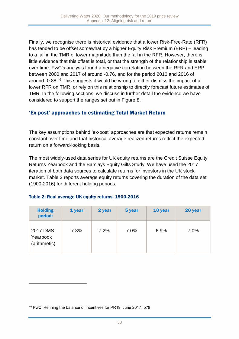
‘Ex-post’ approaches to estimating Total Market Return

The key assumptions behind ‘ex-post’ approaches are that expected returns remain

constant over time and that historical average realized returns reflect the expected

return on a forward-looking basis.

The most widely-used data series for UK equity returns are the Credit Suisse Equity

Returns Yearbook and the Barclays Equity Gilts Study. We have used the 2017

iteration of both data sources to calculate returns for investors in the UK stock

market. Table 2 reports average equity returns covering the duration of the data set

(1900-2016) for different holding periods.

Table 2: Real average UK equity returns, 1900-2016

Holding

period:

1 year 2 year 5 year 10 year 20 year

2017 DMS

Yearbook

(arithmetic)

7.3% 7.2% 7.0% 6.9% 7.0%

46 PwC ‘Refining the balance of incentives for PR19’ June 2017, p78


39

Holding

period:

1 year 2 year 5 year 10 year 20 year

2017 DMS Yearbook

(geometric) 5.5% 5.5% 5.6% 5.6% 6.1%

2017 Equity Gilt Study (arithmetic)

6.9% 6.7% 6.5% 6.3% 6.3%

2017 Equity Gilt Study (geometric)

5.1% 5.0% 5.0% 5.0% 5.4%

Source: Ofwat analysis of Credit Suisse Equity Returns Yearbook (2017) and Barclays Equity Gilt

Study (2017) data

The appropriate length of holding period used to form investor expectations is

difficult to establish definitively. The evidence suggests that equity investors in

privately owned companies typically have investment horizons of at least 5-10 years,

but investors in listed stocks have a mix of investment horizons. We consider it

prudent to focus on periods that are longer than one year due to evidence from

investor surveys, as well as generic investment advice that recommends investors

remain invested in equities for longer than 5 years to reduce the risk of in-year

volatility.47

Averages of historically realised equity returns can be expressed arithmetically or

geometrically. There exists disagreement over which approach is superior. One

argument in favour of an arithmetic mean draws on a conception of historic equity

returns data as a probability distribution which investors use to form expectations of

47 For instance Schroders Global Investor Survey 2016 found average holding periods for private investors was 3 years and 4 years for advisers, but noted this was too short a time period to counteract the volatility associated with equities. Note also https://www.moneyadviceservice.org.uk/en/articles/investing-in-shares, retrieved 05/12/2017

http://www.schroders.com/ru/sysglobalassets/digital/insights/pdfs/2016/sgis-2016/sgis-investment-outcomes-full-report.pdf

https://www.moneyadviceservice.org.uk/en/articles/investing-in-shares


40

future returns – the expected return of a probability distribution is the arithmetic

mean.

Damodaran48 argues that for short forecasting horizons of around 1 year, the

arithmetic average is an unbiased estimator. He argues that for longer periods (such

as 5-10 years), using an arithmetic average is likely to introduce an upwards bias,

due to the widely reported finding that equity returns are negatively correlated.49

Blume (1979)50, Indro & Lee (1997)51 and Jacquier, Kane and Marcus (2005)52 argue

that both arithmetic and geometric averages are biased estimators of long-run

expected returns for forecast periods in excess of next year. They propose a

horizon-weighted average of both arithmetic and geometric averages, with the

weight on the geometric increasing with the time horizon.

Given uncertainty around the average holding period which characterises equity

investors, and a forecast horizon longer than a single year, we therefore consider it

likely that an unbiased ‘ex-post’ range for TMR based on the UK data is likely to lie

between the geometric average TMR range of 5.0-6.1% and the arithmetic average

TMR range of 6.3-7.3%.

In addition to the discussion above, changes in the way RPI is calculated before and

after 2010 have led to a structural increase in the difference between CPI and RPI.

This is due to the differing calculation approaches of the two inflation measures

(commonly known as the ‘formula effect’).53 This has implicitly led to a corresponding

reduction in the yield or cash flow return that investors require on index-linked

48 For example, Damodaran, ‘Equity Risk Premiums (ERP): Determinants, Estimation and Implications – The 2012 Edition 49 For instance, Fama & French, ‘Dividend yields and expected stock returns’, Journal of Financial Economics 22, 1988 50 Blume, ‘Unbiased estimators of long-run expected rates of return’, Journal of the American Statistical Association, 1979 51 Indro & Lee, Biases in Arithmetic and Geometric Averages as Estimates of Long-Run Expected Returns and Risk Premia, 1997 52 Jacquier, Kane and Marcus ‘Optimal estimation of the risk premium for the long run and asset allocation: a case of compounded estimation risk’ Journal of Financial Econometrics, 2005 53 Office for National Statistics, CPI and RPI: increased impact of the formula effect in 2010, 2011

https://www.google.co.uk/url?sa=t&rct=j&q=&esrc=s&source=web&cd=1&ved=0ahUKEwiQ3PbvtoTYAhUD1hQKHaX7CVUQFgguMAA&url=https%3A%2F%2Fwww.ons.gov.uk%2Fons%2Fguide-method%2Fuser-guidance%2Fprices%2Fcpi-and-rpi%2Fcpi-and-rpi--increased-impact-of-the-formula-effect-in-2010.pdf&usg=AOvVaw1PjiQBWN5OKd7aj77gQZNx


41

assets.54 ONS’s latest estimate of this effect is 33 basis points.55 This implies that a

more accurate required return based on this approach can be derived by subtracting

33 basis points from the DMS and Barclays EGS derived averages. Adjusting the

raw data for the ONS’s estimate reduces the range stated above to 4.7-5.7% on a

geometric basis, and 6.0-6.9% on an arithmetic basis.

‘Ex-ante’ approaches to estimating TMR

Various academic studies have criticised the ‘Ex-post’ approach. This body of

evidence argues that estimates of realised return do not provide a reliable basis on

which to base forecasts of Equity Risk Premium (ERP) or TMR. Key sources include:

Mehra & Prescott - who argue that the premium of equity returns over the

Risk-Free Rate for US equity returns data over the period 1889-1978, if

anticipated by investors, is inexplicable in the context of standard economic

models that describe investor risk-aversion.56 This phenomenon is commonly

referred to as the ‘Equity Premium Puzzle’, and is observed in UK equity

returns data, as well as US data;

Fama & French - who argue that US equity returns in the second half of the

20th century were higher than expected. Fama and French base this finding

on a fundamentals-based model of expected returns (‘The Dividend Growth

Model’, or DGM), in which TMR is estimated as the underlying return from the

sum of the average historical dividend yield and the average historical rate of

dividend growth from the S&P 500 index. 57

Dimson, Marsh & Staunton – who consider that long-run historical averages

of returns should be stripped of components of return, which are unlikely to

persist, in order to estimate forward-looking required investor returns. 58 Their

analysis decomposes returns into dividend income, real dividend growth,

expansion of valuation ratios, and changes in the real exchange rate. In their

54 Ofgem, Consultation on our methodology for assessing the equity market return for the purpose of setting RIIO price controls, December 2013, p11 55 Based on the difference between the Dec 2009 (0.54%) and Oct 2017 (0.87%) estimates of the formula effect (Source: ONS) 56 Mehra & Prescott, The Equity Premium, 1985 57 Fama & French, The Equity Premium, The Journal of Finance, 2002 58 Dimson et al. The Worldwide Equity Premium: A Smaller Puzzle, 2006

https://www.ofgem.gov.uk/ofgem-publications/85020/consultationonequitymarketreturnmethodologyletterpdf

https://www.ofgem.gov.uk/ofgem-publications/85020/consultationonequitymarketreturnmethodologyletterpdf

https://www.ons.gov.uk/economy/inflationandpriceindices/timeseries/dra9/mm23

https://papers.ssrn.com/sol3/papers.cfm?abstract_id=891620


42

2017 yearbook, the authors estimate that the real arithmetic risk premium for

a globally diversified investor is likely to be between 4.5-5.0%.59 This implies a

real TMR of 5.4-5.9%, when using the authors’ preferred measure of the

historical world Risk-Free Rate of 0.9%.

Other authors have concluded that UK data provides support for even lower

estimates of the TMR using an ‘ex-ante’ approach:

Gregory (2007)60 applies a Fama-French DGM approach to UK data arguing

that a plausible forward-looking range for UK TMR is likely to be between

4.30% and 6.18% on an RPI-real, arithmetic basis. He bases this calculation

on an Equity Risk Premium ranging between 2.0% and 3.88%, and the

author’s preferred risk-free rate of 2.3%.

Vivian (2007), argues that expected returns implied by a Fama-French DGM

approach since 1966 have been much lower than average stock returns for

the UK stock market as a whole. He concludes that this is primarily due to a

declining investor discount rate during the latter half of the 20th century.

Vivian argues that a better estimate of the expected equity risk premium for

UK investors over the period 1966-2002 was around 3.0% in real terms. This

implies a TMR of 5.09% (based on the author’s use of a Risk-Free Rate of

2.09%), rather than the actual realised returns of 8.9% over the same

period.61

Applying the original Fama-French style DGM approach to the full span of Barclays

Equity Gilt Study data from 1900 to 201662 suggests an unadjusted estimate of

prospective real TMR for the UK of 5.6%.63 By placing more weight on recent years’

role in influencing investor expectations, data from 1990 to 2016 from the same

series yields a lower estimate of 4.2%. Fama & French’s original paper argues that

their dividend growth model has a downward bias due to the dividend growth rate

being less volatile than the rate of capital gain. The authors recommend an uplift

calculated using their proposed corrective factor of half the difference in the

59 Credit Suisse, ‘Credit Suisse Global Investment Returns Yearbook 2017’, February 2017 (p37) 60 A. Gregory, How Low is the UK Equity Risk Premium?, 2007, 61 A, Vivian,The Equity Premium: 101 Years of Empirical Evidence from the UK, 2007, p30 62 Calculating the sum of the average dividend yield and average dividend growth rate over the assessed period. 63 Source: Ofwat analysis of Barclays Equity Gilt Study Data 2017



43

variances of share price growth rate and dividend growth rate, respectively.64 This

results in an adjusted range of 5.1% (1990-2016) to 6.3% (1900-2016). We note in

the following section that the case for making this adjustment is greatly weakened if

we consider the relative variances of total equity yield (that is dividends and share

buybacks) and share price growth. PwC’s analysis suggests that the former has

been more volatile than the latter in almost all years since 2004 except for the last

few months of 2017.65

Forward-looking approaches – the Dividend Discount Model

The Dividend Discount Model (DDM) combines assumptions about dividend growth

with data on share prices to estimate an investor discount rate, based on the

principle that a share’s price should reflect the present value to investors of its future

dividend payments. When the share price data is of a sufficiently broad stock market

index, the resulting discount rate can be used as an estimate of TMR. The approach

is widely used to set the cost of equity in US economic regulation.

A basic model of share prices assumes that an investor values a share as the

stream of dividend payments discounted to its present value, using their discount

rate.

P0 = D1/(1+r) + D2/(1+r)2 + D3/(1+r)3 … Dt/(1+r)t …

Where P0 is the present value of a stream of dividends (D1, D2, D3, … Dt…) at times

(1, 2, 3… t…), which are associated with asset P, and where r is the investor’s

discount rate, or required return.

Where dividends grow at a constant rate, ‘g’, this equation reduces to

P0 = D1/(r-g)

This can be rearranged to:

r = D1/P0 + g

64 Fama & French, The Equity Premium, The Journal of Finance, 2002, p654 65 PwC, Updated analysis on the cost of equity for PR19, December 2017, p15


44

D1 can be replaced by D0 (1+g), where D0 is the most recent dividend paid. For any

given assumption about g, the formula provides an estimate of r.

This simple model assumes a constant growth rate. It is called a one-stage model.

Multi-stage models utilise different dividend growth rates for the short run and long

run.

For our draft methodology proposals, we commissioned PwC to derive estimates of

TMR using their own Dividend Discount Model. The (nominal) rate reported by their

DDM analysis at March 2017 was 8.3%, with a five year rolling average to that point

of 8.8%.66

Several respondents to our draft methodology proposals criticised the approach

taken by PwC, with most commentary focusing on the following issues:

Volatility of modelling outputs – arguing that spot estimates from the

models were too volatile to rely on for a TMR assumption, which would apply

over the 5 year period for the price control;

Subjectivity of the dividend growth assumption – arguing that other

plausible alternatives to PwC’s assumptions around dividend growth exist and

would result in a higher TMR, if used (for example analyst forecasts of

dividend growth - as used by the Bank of England); and

Omission of a volatility uplift – that by modelling investor value as entirely

as a function of dividends, PwC failed to incorporate compensation investors

would require due to the higher volatility observed in underlying share prices.

We recognise that the output of the DDM is sensitive to the choice of assumption

around dividend growth. There exist multiple sources, which can be used to

determine the growth assumption. Table 3 sets out our assessment of three

commonly-used sources of data for the dividend growth assumption:

Table 3: Dividend growth assumptions for the DDM

66 PwC ‘Refining the balance of incentives for PR19’ June 2017



45

Dividend growth

assumption:

Advantages: Drawbacks:

1) Historical dividend

growth rates.

Based on empirically

observed data.

May not represent

forward-looking

expectations and so

misrepresent forecast

TMR.

2) Analyst forecasts

of dividend growth.

In theory more closely

tied to market

expectation of dividend.

Analyst sentiment may

not perfectly represent

investor sentiment

There is a large body of

evidence suggesting that

these forecasts suffer

from optimism bias.

3) GDP growth rate

forecasts.

A plausible long-term

upper bound growth rate,

as dividend growth

cannot indefinitely

outstrip GDP growth.

Subject to forecast error

Imperfectly understood

relationship between

expected GDP growth

and expected dividend

growth.

We commissioned new 2017 DDM-based estimates from PwC and Europe

Economics to inform our view of TMR, with each organisation using its own

assumptions and approaches. Table 4 sets out the key characteristics of these

models.

Table 4: PwC and Europe Economics Dividend Discount Models: Key Characteristics

and Assumptions

Model and originating

institution

Key features of the model

1) PwC multi-stage

GDP-based DDM

Nominal terms model operating on nominal inputs

and estimating nominal TMR

Based on FTSE All-Share index, includes buybacks;

Dividend growth assumption based on UK GDP

growth forecasts from Office of Budget

Responsibility and Consensus Economics; and


46

Different dividend growth rate assumption for short

term (<5 years) and long-term (>5 years).

2a) Europe Economics

multi-stage GDP-based

DDM (November 2017)

CPI-real model operating on CPI-real inputs

converted from nominal ones and estimating a CPI-

real TMR


Dividend growth assumption based on UK GDP

growth forecasts and forecasts from the IMF; and


term (<5 years) and long-term (>5 years).

2b) Europe Economics

multi-stage GDP-based

DDM (November 2017).

Same as 2a) but with GDP growth forecasts deflated

using expected inflation, rather than the outturn.

3) Europe Economics

multi-stage historic

dividend growth-based

DDM.

CPI-real model operating on CPI-real inputs

converted from nominal and estimating CPI-real

TMR


Dividend growth assumption provided by outturn

dividend yields and growth from FTSE All-Share;


term (<5 years) and long-term (>5 years); and

Source: PWC, Europe Economics analysis

Table 5 below summarises the results from models created by PwC and Europe

Economics. These results have been tabulated in nominal, RPI and CPIH terms.

Because PwC’s model operates on data in nominal terms, we have used our long-

term assumptions of 3.0% RPI and 2.0% CPIH inflation to deflate the nominal

estimates to real-terms counterparts. Europe Economics’ model operates on data in

CPI-real terms. Nominal and RPI counterparts are derived by inflating their CPI-real

estimates by 2.0% and deflating by 1.0%, respectively.


47

Table 5: PwC and Europe Economics Dividend Discount Models: Results67

Model and date of

estimate

TMR range

(Nominal)

TMR range

(Real, RPI)

TMR range

(Real, CPIH)

1) PwC multi-stage

GDP-based DDM

(Dec 2016) 8.3-8.8%

5.1-5.6%

6.2-6.7%

1) PwC multi-stage

GDP-based DDM

(Oct 2017) 8.4-8.7%

5.2-5.5%

6.3-6.6%

2a) Europe

Economics multi-

stage GDP-based

DDM

(Mar 2017)

8.0-9.0%

4.9-5.9%

5.9-6.9%

2b) Europe

Economics multi-

stage GDP-based

DDM

(Mar 2017)

8.3-8.9%

5.1-5.8%

6.2-6.8%

3) Europe

Economics multi-

stage historic

dividend growth-

based DDM.

(Mar 2017)

7.3-8.3%

4.2-5.1%

5.2-6.2%

Overall range for

5yr rolling

averages 8.3-9.0%

5.1-5.9%

6.2-6.9%

67 Except for the final row, TMR ranges are expressed using the spot figure and the 5-year trailing average on the month of estimation for each end of the range.


48

Source: PwC, Europe Economics analysis

Our view, supported by both PwC and Europe Economics, is that more weight

should be placed on multi-year trailing averages of DDM outputs to inform point

estimates of TMR. This serves to reduce the volatility in TMR estimates which would

otherwise result. However, we note that for all models, we have reviewed that spot

values lie below the 5 year averages. If this trend were to continue in future years, it

would imply a downward movement in the trailing average, when calculated for draft

and final determinations. Overall, the range of outputs for TMR using 5-year

averages is relatively narrow – ranging from 5.1-5.9% in real RPI terms.

In its response to our the draft methodology proposals, National Grid provided an

estimate of TMR inferred from the Bank of England’s published Equity Risk Premium

(ERP) point estimates from its multi-stage DDM,68 and calculated by Bloomberg. The

response states that, for December 2016, the Bank of England’s modelled outputs

implied an RPI-real TMR of 7.1-7.7%, and Bloomberg’s TMR was 8.0%. In

subsequent correspondence with us,69 National Grid revised the upper end of the

range for its Bank of England estimate to 7.4% on the understanding that the Bank’s

approach uses spot curves for the risk free rate, rather than forward curves, which

underpinned its calculation of 7.7%. The Bank of England DDM is based on the

FTSE All-share index, with short term dividend growth forecasts provided by

aggregated firm-level forecasts, and long-term forecasts based on UK GDP growth.

We understand that Bloomberg’s model is also multi-stage, but is based on the

FTSE 100 rather than the FTSE All-Share – and that it also relies on analyst growth

forecasts.

The estimates of TMR from Bank of England and Bloomberg DDMs are higher than

the range of estimates we have derived using ‘ex-post’ approaches on historical data

(see Figure 7) – which themselves lie towards the high end of our overall range of

TMR estimates. We consider that the key factor explaining the much higher Bank of

England and Bloomberg DDM results are their use of analyst forecasts70 as an input

for forecast dividend growth. A large body of academic work exists to support the

view that analyst-derived forecasts of future earnings are prone to optimism bias and

68 Bank of England, An improved model for understanding equity prices (visual summary) 69 Email from National Grid to Ofwat, 12/10/2017 70 The Bank’s model uses Institutional Broker’s Estimate System (IBES) forecasts.


49

overreaction to new economic data. 71 The Bank’s working paper72 describing its

revised model notes that its reliance on analyst forecasts is ‘a key source of potential

error in the DDM’. We do not therefore consider either model as appropriate to

inform central estimates of TMR for the purposes of setting price determinations.

Our view, supported by the approaches adopted by PwC and Europe Economics, is

that GDP growth forecasts and historic dividend growth serve as a reasonable proxy

for future rates of dividend growth in the DDM models we have reviewed. The

Competition Commission in 2014 concluded, based on a review of UK data between

1900 and 2010, that the rate of real dividend growth was 0.5%, compared with real

GDP growth of 1.89% over the same period73. This could mean that GDP-based

DDM estimates may in fact overstate actual investor TMR.

In a report commissioned as part of three regulated firms’ response to our

consultation, KPMG argued that PwC’s DDM estimates a geometric average return

as its estimate for the TMR, which fails to compensate investors for volatility in their

capital investment.74 KPMG refers to original work by Fama & French in 200275 and

the Competition Commission’s redetermination of Northern Ireland Electricity Price

Limited’s price limits in 2014.76 In the former paper, the authors argue that outputs

from their Dividend Growth Model are likely to understate expected returns by failing

to recognise that volatility in share price growth has historically been higher than

volatility in dividend growth – thereby undercompensating investors for risk. Fama &

French recommend an adjustment of half the difference between the historical

variance of the growth rates of dividend growth and share price growth, to

compensate for this bias. The Competition Commission said this implied an uplift of

75 basis points.

71 Eg De Bondt & Thaler, ‘Do security analysts overreact’ (1990), or Chan et al, ‘The Level and Persistence of Growth Rates’ (2003) (both using IBES data). 72 Bank of England, Quarterly Bulletin, Topical article, An improved model for understanding equity prices, Quarterly Bulletin 2017 Q2. 73 CC (2014), ‘Northern Ireland Electricity Limited price determination’, final determination, para 13.154. The CC found that the historical growth rate of dividends for the UK was 0.5% between 1900 and 2010 compared with real GDP growth of 1.89% over the same period. 74 KPMG, A review of Ofwat’s proposed approach to total market returns, August 2017 75 Fama & French, The Equity Premium, The Journal of Finance, 2002 76 Competition Commission (2014), ‘Northern Ireland Electricity Limited price determination’, final determination, A13(2)-4

http://lsvasset.com/pdf/research-papers/Level+Persistence_of_Growth_Rates_FINAL.pdf

http://lsvasset.com/pdf/research-papers/Level+Persistence_of_Growth_Rates_FINAL.pdf

https://www.bankofengland.co.uk/-/media/boe/files/quarterly-bulletin/2017/an-improved-model-for-understanding-equity-prices.pdf?la=en&hash=F0385353B45A130A1AA557165FBEC5E326FD57FB

https://www.bankofengland.co.uk/-/media/boe/files/quarterly-bulletin/2017/an-improved-model-for-understanding-equity-prices.pdf?la=en&hash=F0385353B45A130A1AA557165FBEC5E326FD57FB


50

Europe Economics considered the issue of the volatility adjustment in its report.77 It

argues there is no intrinsic reason why GDP growth could not be conceived as

providing a direct estimate of average capital growth, as well as serving as a proxy

for dividend growth. In this case, it argues that the issue of a variance effect does not

arise — average GDP growth is providing a direct estimate of (arithmetic) average

capital growth.78 For models based on dividend growth, Europe Economics

considered the need for a volatility adjustment. It concludes the wedge between the

volatility in dividends and buybacks and that in capital values had fallen in recent

years and suggested on some measures, dividend and buyback volatility may even

be higher than volatility in capital values. Europe Economics did not include a

volatility adjustment in their dividend growth model, but stated that even if a volatility

adjustment were included, it would be less (probably materially less) than the 75bps

the Competition Commission used in the past and would take the results for the

dividends-based model no higher than the results for the GDP-based model.

Using 2006-2017 data from the FTSE All-Share, PwC argue that once share

buybacks are accounted for, the variance in total investor equity yield (i.e. dividends

plus buybacks) is greater than variance in share price growth for almost the entirety

of the period.79 PwC thus find that the variance adjustment turns negative due to a

higher total equity yield growth volatility compared to total nominal capital growth

volatility. They therefore argue there is no downward bias and hence no need to

apply the Fama & French adjustment to the DDM for forward-looking purposes.

On the basis of work by PwC and Europe Economics, we therefore conclude that it is

unnecessary to apply an uplift to the estimates of TMR reported by the Dividend

Discount Models in our review.

Forward-looking approaches – Market to Asset Ratios

Market-to-Asset Ratios (MARs) are defined by the ratio of a company’s Enterprise

Value80 to its Regulatory Capital Value (RCV). A positive MAR means that investors

are willing to pay more for their equity share than the value implied by the equity

77 Europe Economics (2017), ‘PR19 — Initial Assessment of the Cost of Capital’, December 2017, p31-32 78 Europe Economics (2017), PR19 — Initial Assessment of the Cost of Capital 79 PwC, Updated analysis on the cost of equity for PR19, December 2017 80 Defined as market capitalisation plus net debt


51

share in the RCV at the same level of gearing. This premia could be explained by

expected outperformance from various elements of the price control such as the

allowed return and totex.

We have seen significant premia in private transactions since 2010 (MARs for some

private transactions have exceeded 1.5 and analysts have estimated MARs of up to

around 1.3 for the listed stocks). PwC’s analysis of transactions over 1998-2017 also

found that MARs in recent years have risen significantly above the average multiple

of 1.24 for the period. It is difficult to explain these multiples based on measures of

cost and financial incentive outperformance.

One potential explanation is that a component of MAR premia is due to investor

expectations of outperformance against the allowed cost of equity. For our draft

methodology proposals, we asked PwC to test this hypothesis by stripping out the

contribution of other sources of outperformance from the MAR premium observed in

two listed water companies with predominantly regulated business activities –

Severn Trent and United Utilities. A focus on these listed companies, rather than

unlisted companies or Pennon, is appropriate due to the frequency of share trading

giving better availability of Enterprise Value data over time, the fact that these

companies are virtually pure-play water companies and there being lower potential

for confounding influences (for example the ‘control premium’ associated with equity

prices in private equity acquisitions).

Market analysts publish expectations of outperformance on key components of the

revenue allowance (totex, ODI, SIM and debt financing) for the listed companies. To

derive an estimate of the investor cost of equity implied by the premium to RCV

calculation, PwC calculated future cashflows from an analyst forecast of

outperformance and subtracted their present value from the excess of the enterprise

value over the RCV at March 201681. They then calculated a discount rate, which

explains the residual excess value as the margin between the regulatory allowance

for the cost of equity and the investor discount rate (assumed to be their actual cost

of equity). By applying assumptions for a Risk-Free Rate and equity beta82,

81 PwC ‘Refining the balance of incentives for PR19’ June 2017 82 These assumptions were a nominal RFR of 1.5% or 3.0% and a re-levered equity beta of 0.8, consistent with the PR14 assumption



52

estimates of Total Market Return can be derived for comparison with other

approaches.

PwC derived nominal estimates in the range of 7.6-8.1%, depending on the point

estimate of risk-free rate used, and whether the calculations were carried out on the

share price of United Utilities or Severn Trent.83

PwC’s approach to their MAR analysis drew criticism on three key grounds:

Subjectivity of outperformance assumptions - that judgments on the

contribution of specific factors to outperformance (and hence share price) are

subjective and therefore unreliable;

Omission of other contributions to outperformance - that the analysis

failed to capture the impact of sources of outperformance other than the cost

of equity (in particular: RCV growth, non-regulated revenue and financing

outperformance). This would affect the inferred investor cost of equity; and

Unrepresentativeness of the listed companies - some respondents argued

that the listed companies were particularly high performers in various

categories of cost outperformance and so inferences could not be drawn to

the rest of sector. It was also argued that, as a whole-market variable, TMR

could not be inferred from the cost of equity of one or two companies.

We recognise that the MARs approach is dependent on analyst assessments of

future outperformance and judgment over how long this will apply. There is some

uncertainty around these parameters. The source of the outperformance estimates is

however, independent. We continue to consider that MARs analysis provides a

valuable source of information and that it is appropriate that we take it into account in

assessing our overall estimate of the TMR.

PwC’s original analysis included assumptions for debt outperformance and RCV

growth. PwC has updated its analysis to include the effect of the Capital Incentive

Scheme (CIS) downward adjustment to the 2020 RCV84 and the effect of non-

83 Severn Trent provided the low end of the range with a nominal RFR assumption of 3.0%, and United Utilities provided the high end of the range with a nominal RFR assumption of 1.5%. Both calculations assumed an asset beta of 0.3, consistent with the assumption made at PR14. 84 See Ofwat PR14 reconciliation rulebook, 2016

https://www.ofwat.gov.uk/wp-content/uploads/2016/10/PR14-reconcilliation-rulebook1.pdf


53

regulated activities 85. In addition to this, we asked Europe Economics to give its view

of the MAR premium, updated to March 2017 levels.

Table 6: Updated results from MARs analysis

Organisation Nominal TMR range

PwC86. 7.5-8.2% (estimated March 2016 data).

Europe Economics.87 7.4 – 8.6% (estimated using March 2017 data).

Figure 9 shows the evolution of MAR premia over the course of 2017. Falls since

June of this year have moved the observed MAR premium to below the range, which

PwC’s analysis predicts based on non-equity sources of outperformance for United

Utilities and Severn Trent (1.14 and 1.15, respectively). A range of factors could

have caused this fall, including the debate about potential nationalisation of utilities.

It may also reflect a reduction in investor expectations of equity outperformance,

following our programme of investor engagement in the first half of this year, though

we note MARs remain positive88.

85 Assumed to be 3%, based on KPMG estimate for SVT. See KPMG (2017), ‘A review of Ofwat’s proposed approach to total market returns’, P32 86 PwC, Updated analysis on the cost of equity for PR19, December 2017, 87 Europe Economics (2017), ‘PR19 — Initial Assessment of the Cost of Capital’, December 2017 88 For instance, Jonson Cox Keynote Speech at the Water UK City Conference on 9 March 2017 “…the cost of equity for stable mature well-regulated infrastructure assets has fallen markedly. Listed water companies are currently trading at around a 25% premium implying a nominal cost of equity of under 7%. We have seen institutional transactions at premia well above those observed in the market for the listed stocks. These transactions tell us that investors are willing to accept a cost of equity even below these levels…”

https://www.ofwat.gov.uk/wp-content/uploads/2017/03/Water-UK-City-Confererence-Keynote-Speech.pdf


54

Figure 9: Premium of enterprise value89 over Regulatory Capital Value

Forward-looking approaches – Other evidence

In addition to approaches that focus on using market-data to infer an estimate of

TMR, we provide a review of more qualitative evidence on its future level, provided

by statements from investment professionals and academics.

Evidence from the recent Credit Suisse Yearbook points to expectations that future

equity returns will be lower than the historical average. The Credit Suisse Yearbook

states, for example, ‘since real interest rates remain at low levels, this is likely to

depress returns on all asset classes – including equities. Given that equity investors

made a 4.2 percentage point higher return than money market investors in the 1900-

2016 period, the authors predict an additional real return of just 3 to 3.5 percent in

the years ahead’90. To support their claim, the authors make use of historical multi-

89 Enterprise value is defined as book value of net debt plus the market value of shares 90 Credit Suisse, ‘Low interest rates hit returns on equities’, April 2017

0%

5%

10%

15%

20%

25%

30%

35%

Feb-17 Mar-17 Apr-17 May-17 Jun-17 Jul-17 Aug-17 Sep-17

Severn Trent United Utilities


55

country returns data, which shows that periods of low real interest rates have

historically been associated with periods of low equity returns.91

In a UK context, recent statements from infrastructure investors suggest that

required returns have adjusted downwards. For example, figure 10 presents data

from HICL Infrastructure Company (HICL). It shows that the discount rates HICL has

used for UK infrastructure assets have declined since March 2012.

Figure 10: HICL UK infrastructure discount rate, 2012 to 2017

Source: Ofwat analysis from HICL reports92

We acknowledge that HICL invest in a range of assets, including outside of the water

sector. However, the chart shows changes in the equity risk premium and risk free

rate over time, with a general trend of a falling total market return. It thus supports

91 Credit Suisse, ‘Global investment returns yearbook 2017 – slide summary deck’, slide 11 92 See for example, page 47 HICL Infrastructure, Delivering Real Value, Annual Report and Financial Statements 2017

3.3% 2.9% 2.9%3.4% 3.4% 3.0%

2.2% 2.4% 2.2%1.4% 1.7% 1.8%

8.6% 8.5% 8.4% 8.3% 8.2% 8.0% 7.8% 7.7% 7.5% 7.3% 7.2% 7.3%

0%

2%

4%

6%

8%

10%

Ma

r-1

2

Sep-1

2

Ma

r-1

3

Sep-1

3

Ma

r-1

4

Sep-1

4

Ma

r-1

5

Sep-1

5

Ma

r-1

6

Sep-1

6

Ma

r-1

7

Sep-1

7

Average long-dated Government bond yield Average risk premium


https://www.hicl.com/sites/default/files/AnnualReportandFinancialStatementstoMarch2017.pdf

https://www.hicl.com/sites/default/files/AnnualReportandFinancialStatementstoMarch2017.pdf


56

the view that the Equity Risk Premium does not fully offset the impact of a falling

Risk Free Rate when considering the return that investors expect.

A similarly cautious view about prospects for equity investors can be found in

statements from asset manager Blackrock, which publishes its view of expected

returns for investors in its funds in different localities and asset classes. Over the

next 5 years, it expects an annualised nominal arithmetic return for UK investors in

large UK companies of 7.4%, and for global infrastructure equity of 6.0%93. Their

longer-term assumptions change to 7.1 and 7.4% respectively.

Schroders set out a similarly cautious view. While its survey94 of 22,000 people

internationally suggested a global average expected return of 10.2%, separate

analysis by the Schroders Economics Group, forecast returns of 4.2% (nominal) for

world stock markets. Similarly, while its survey suggested return expectations of

8.7%, the Schroders Economics Group forecast nominal UK stock market returns of

5.4%95 (3.0% real) a year to 2024.

In their 41-country survey of finance and economics professionals and academics,

Fernandez et al (2017), found that the average stated country-level TMR (based on

91 UK respondents) was 8.1% in nominal terms. 96

Consistent with the approach adopted in previous regulatory determinations, we use

the evidence gathered from investor surveys, economic forecasts and other sources

only as a cross check to our view of the TMR rather than to directly inform our view.

This evidence does however support the view that expectations of TMR from some

quarters are even lower than the point estimate we apply in our early view.

93 On an arithmetic basis, over a 5-year horizon. Long-term equilibrium returns are assessed to be 7.0% for large UK companies and 7.4% for global infrastructure equity. Source: https://www.blackrock.com/institutions/en-us/insights/portfolio-design/capital-market-assumptions accessed on 06.11.2017 94 Schroders, Global Investor Survey, 2017 95 Schroders, Global Market Perspective, Economic and asset allocation views, Q4 2017 96 P. Fernandez et al, ‘Discount rate (Risk-Free Rate and Market Risk Premium) used for 41 countries in 2017: a survey’, 2017

https://www.blackrock.com/institutions/en-us/insights/portfolio-design/capital-market-assumptions

http://www.schroders.com/en/sysglobalassets/digital/insights/2017/pdf/global-investor-study-2017/theme2/schroders_report-2__eng_master.pdf

http://www.schroders.com/getfunddocument?oid=1.9.2436437




57

5.5 Evidence on Equity Beta for 2020-25

The equity beta is a measure of how a share’s returns co-vary with undiversifiable or

market-wide risks (for instance, increases in interest rates). Equity beta is also

assumed to vary in proportion to the level of gearing in a company, as higher gearing

reduces resilience to market-wide risks.

Equity beta is an important component of the Capital Asset Pricing Model (CAPM)

framework, which concludes that investors only require compensation for market-

wide risks, not firm-specific risks. This is because investors can eliminate firm-

specific risk by diversifying and holding a larger portfolio of investments. In a large

portfolio, it is argued, these effects will average out to zero, on the basis that weak

performance in some companies will be cancelled out by strong performance in

others.97

Market-wide risks cannot be hedged in the same way, but the nature of a firm’s

activities will imply a particular level of exposure to market-wide risk. The CAPM

states that equity investors in firms with a lower level of exposure to market-wide

risks are more protected from these risks, and so require a lower return on equity.

Equity betas are estimated by regressing stock returns against market returns. The

resulting equity beta will reflect the firm’s financial gearing over the estimation period,

and the underlying business risk. The latter is called the asset beta. The asset beta

is typically calculated by adjusting the initial market-derived equity beta to strip out

the contribution of gearing. The level of asset beta derived via this approach will also

depend on the assumption used for debt beta (which measures how debt returns for

the relevant company co-vary with market-wide risks).

5.5.1 Debt beta

Europe Economics consider that returns to debt as well as equity bear some risk in

response to market-wide risks. This is because there is usually a degree of

correlation between the risk of default and the economic cycle – companies are more

likely to fail in a downturn, negatively affecting returns to their bondholders. In its

view, this means that it is likely that some of the debt premium (the excess of the

97 A. Damodaran, Models of Risk and Return, accessed on 06/12/2017

http://people.stern.nyu.edu/adamodar/pdfiles/ovhds/ch3.pdf


58

cost of new debt over the risk-free rate) arises because of correlation between these

market-wide risks, rather than the company or sector-specific risk of default. Europe

Economics argues that this justifies the incorporation of a positive debt beta when

performing the calculation required to derive the asset beta from equity market data,

and when deriving an estimate of the ‘re-levered’ equity beta of a water company at

our chosen notional gearing of 60%. The Competition Commission also adopted a

debt beta in its 2010 re-determination of Bristol Water’s price control.98

As recognised in previous price controls99, the use of a debt beta only has a material

impact on the equity beta calculated for the notional company when there is a non-

trivial difference between the actual gearing of companies providing the estimate of

beta and the notional gearing. In this case, Europe Economics report the enterprise

value gearing of Severn Trent and United Utilities as 47% and 51%, respectively.

Compared to our gearing assumption for the notional company of 60%, as this is a

non-trivial difference, we have decided to adopt a debt beta assumption consistent

with Europe Economics’ approach.

Europe Economics consider a debt beta of 0.2 is most likely to be accurate, but cite

regulatory decisions which have tended to favour values in the 0.1 to 0.15 range for

debt beta, ultimately choosing 0.125 as their point estimate.100 We have chosen 0.1

for our point estimate of debt beta in our early view. This is a cautious approach as

there have been no defaults in the water sector since privatisation. The fact there

have been no defaults does not mean that no debt beta should be taken into account

as, for example, bonds carry credit ratings which incorporate an assessment of

default risk. However, it does mean there is a scarcity of empirical data to

decompose the risk premium into components due to the default rate and the

influence of market-wide risk. Our assumption is consistent with the debt beta used

by the Competition Commission in the Bristol Water determination cited above.

98 Competition Commission, Bristol Water PLC Price Determination - Appendices, N32, February 2010 99 Ofwat, ‘Setting Price Controls for 2015-20 - Risk & Reward Guidance’, January 2014 (p18) 100 Europe Economics (2017), ‘PR19 — Initial Assessment of the Cost of Capital’, December 2017

http://webarchive.nationalarchives.gov.uk/20130104172625/http:/www.competition-commission.org.uk/assets/competitioncommission/docs/pdf/non-inquiry/rep_pub/reports/2010/fulltext/558_appendices.pdf

https://www.ofwat.gov.uk/publication/europe-economics-pr19-initial-assessment-cost-capital/


59

5.5.2 Equity beta for the notional company

As stated above, betas are estimated via regression analysis as the correlation of

equity returns with the wider stock market – usually taken to be the FTSE All-Share

in a UK context. Previous regulatory determinations have considered daily, monthly

or yearly data, and use a ‘trailing window’ encompassing 1, 2 and 5 years’ worth of

data. We derive an asset beta from this initial estimate by stripping out the

contribution of gearing to shareholder risk, where gearing is defined as net debt to

enterprise value.

Figure 11 shows asset betas for the two remaining listed UK water companies with

predominantly regulated activities, assuming a debt beta of 0.1101.

Figure 11: Asset betas for listed UK water companies, (daily data, 2010-2017)

Source: Thomson Reuters Datastream and Ofwat analysis

We note from the CMA’s 2015 redetermination of Bristol Water’s price control that

the correct frequency of data to use when estimating beta remains a topic of debate.

The CMA noted some academic studies that found evidence of downwards bias

when using daily data, though it did not find evidence of this in its own

calculations.102 Europe Economics consider that estimates based on daily data are

101 We do not consider the inclusion of Pennon (owner of South West Water) to improve our estimates of beta due to its large waste management division. 102 Competition and Markets Authority, Bristol Water Plc Price Determination – Appendix 10, A10(1)-22

https://assets.publishing.service.gov.uk/media/5627997640f0b60368000001/Appendices_5.1_-_11.1_and_glossary.pdf


60

better than those derived using weekly or monthly data as they rely on larger sample

sizes and are more precise, having narrower confidence intervals. We have

accordingly used daily data for our preliminary view on equity betas.

Asset betas derived using a short trailing window may be distorted by specific events

(for example any uncertainty associated with the price review process itself).

However, a trailing window which is too long risks including historic data with limited

relevance to a forward-looking estimate of beta (for example data from price control

periods with different regulatory frameworks). We believe that a 2 year trailing

window represents an appropriate balance, capturing only market data from the

current control period, though we note that the use of both 2 and 5 year trailing

windows yield broadly similar estimates (Figure 11).103

We therefore focus on 2 year betas using daily data to derive our estimate of asset

beta for our early view – 0.37. This estimate incorporates a debt beta of 0.1. The

asset beta derived using a PR14 approach of using a debt beta of zero would be

0.32. We have noted Europe Economics’ approach of choosing a working value of

0.3104 based on its view in the round that market-derived estimates do not

convincingly point to an increase over the PR14 assumption, but for our early view

we prefer an approach more grounded in market-derived estimates.

In table 7 we show the derivation of our estimate, and (for comparison purposes) the

derivation of beta using our approach at PR14.

103 Figure 11 shows there is however little difference between the latest point estimates derived from 2 and 5 year trailing windows. 104 Prior to applying debt beta assumption


61

Table 7: Comparison of our early equity beta view and PR14

Calculation Ofwat early

view

Illustration with

a debt beta of

zero

PR14

Observed

equity

beta105.

A 0.63 0.63 -

Observed

Gearing106

B 49% 49% -

Asset beta

(not reflecting

debt beta)

C = A x ( 1 – B ) 0.32 0.32 0.3

Debt beta. D 0.1 0 0

Asset beta

revised for

debt beta.

E = C + D x B 0.37 0.32 0.3

Notional

gearing.

F 60% 60% 62.5%

105 Observed beta is an average of the Severn Trent and United Utilities observed equity betas of 0.62 and 0.64, respectively, as reported on 31/07/2017 106 Observed gearing is an average of the Severn Trent and United Utilities observed gearing of 47% and 51%, as reported on 31/07/2017


62

Re-levered

beta.

G = ( E – ( F x D

)) / ( 1 – F )

0.77 0.80 0.80

Source: Ofwat calculations using Thompson Datastream Data

We note there are alternative approaches to estimating beta, for example, as set out

in the cost of capital report by Economic Consulting Associates prepared for

CCWater.107 Together with the availability of more recent market data, this means

we will need to update and reconsider the evidence on equity beta when we set the

cost of capital for draft and final determinations in 2019.

5.5.3 Forward-looking beta estimates for 2020-21 – 2024-25

Several responses to our draft methodology proposals expressed the view that

proposed changes to the regulatory framework for PR19 were likely to increase or

decrease beta. They argued that these changes ought to be reflected in our forward-

looking beta assumption, rather than just relying on recent market data.

As discussed at the start of section 5.5, under the CAPM, beta is a measure of

exposure to market-wide risk. We therefore consider in table 8 the arguments put

forward by respondents and our view of how they could change the exposure of

equity investor returns to market wide risks.

107 Economic Consulting Associates, Recommendations for the Weighted Average Cost of Capital 2020-2025, 27 November 2017




63

Table 8: Company representations on forward-looking beta and our response

Issue raised Respondent Argued

impact on

beta

Response

Greater focus on

recent data when

estimating TMR will

increase

covariance of

sector returns with

the benchmark

index.

SEW Increase

Increases to the cost of

finance are an economy-wide

risk. Using recent evidence to

inform this component of

financing costs, should

provide greater protection

from market risks as it is likely

to better align the allowed

return to the expected return

(that is rising TMR) – and this

should reduce beta.

Increased

cyclicality of

returns, driven by

cost of debt

indexation.

SEW Increase

Increases to the cost of

finance are an economy-wide

risk. Using recent evidence to

inform this component of

financing costs, should

provide greater protection

from market risks (that is

rising interest rates) – and this

should reduce beta. This view

is also set out by Europe

Economics.

Increased

cyclicality of

returns driven by

cost of debt

indexation.

CCWater Decrease

Introduction of

more competition

in water resources

and bioresources,

SEW, SSC Increase

Increased competition is a

diversifiable risk (one firm’s

loss of market share is

another’s gain). Thus, there

should be no increase to beta.


64

will increase risks

to investors.

Switch from RPI to

CPI indexation

SEW Increase

Firms will continue to be

largely protected from inflation

risk through indexation of their

revenues and RCV. It is not

clear how use of a less

volatile, more accurate

measure of inflation increases

exposure to this category of

market-wide risk. We consider

it unlikely there would be any

material, robustly quantifiable

impact on the on the

industry’s risk (and hence

financing costs).108

More challenging

targets for

efficiency and

service

performance

SEW Increase

Greater risks are likely to arise

at the company-level, hence

such risks should be

diversifiable and should not

affect beta.

Overall, we conclude that there is some evidence that beta is reduced by proposed

changes in our draft methodology proposals. In keeping with the similar conclusion

reached by Europe Economics for our early view, we have decided against an ‘ex-

post’ adjustment to the beta we have derived from market data. This is because the

size of the appropriate downward adjustment is unclear.109

108 See Oxera, Indexation of future price controls in the water sector, 31 March 2016 109 Europe Economics (2017), ‘PR19 — Initial Assessment of the Cost of Capital’, December 2017

https://www.oxera.com/getmedia/151823cd-c92c-4394-be5e-ea97312df1a5/Oxera_Indexation-of-future-price-controls-in-the-water-sector.pdf.aspx?ext=.pdf


65

5.6 Evidence on the Risk-Free Rate for 2020-25

The Risk Free Rate (RFR) is an estimate of the return that investors require for

investing their money at no risk to the amount invested. It is an important component

in the CAPM framework, as it provides the minimum return investors require, before

considering any additional premium due to the risk characteristics of a particular

investment.

It is common UK regulatory practice to assume that the yield on UK government

bonds (or ‘gilts’) is a suitable guide to the RFR, given their liquidity and negligible

default risk.110

Figure 12 shows that nominal spot yields for 5, 10 and 20 year gilts have followed a

declining path since 2010. Yields for 10 and 20 year bonds were 1.20% and 1.91%

in March 2017, respectively. Given uncertainty over the average investment horizon

for equity investors, we conservatively focus on the higher-yielding 10 and 20 year

zero-coupon111 nominal gilts to inform our early view of the RFR.

110 Moodys’ analysis of sovereign default rates between 1983 and 2016 shows that no country with a rating ‘Baa’ or above defaulted on sovereign debt. The UK’s current rating is ‘Aa2’- 5 notches above. 111 Zero-coupon gilts are more risk-free than coupon bearing bonds as investors do not face risk from reinvesting coupon payments.

https://www.researchpool.com/download/?report_id=1416505&show_pdf_data=true


66

Figure 12: Yields on zero-coupon nominal UK government bonds, 2010-2017

Source: Bank of England

Some respondents to our draft methodology proposals argued for an upwards

adjustment to estimates of the RFR derived using gilt yields. Respondents argued

that recently observed yields are not a suitable guide to the yield that typical

investors are expecting for investing in a risk-free asset. These respondents cited in

particular, the Bank of England’s purchases of gilts over the course of successive

waves of its Quantitative Easing programme.112

We do not agree with this assessment. The Bank’s retrospective analysis of its

programme show that although the initial gilts purchase announcement may have

reduced yields on long-term gilts by around 100 basis points, the response to

successive waves has been more muted. For some QE announcements, long and

short-term yields increased in response. 113 Gilt yields also continued to fall between

2013 and 2016, when the Bank’s Asset Purchase Facility was not increasing its

holdings of gilts.114

112 The purpose of this programme is to increase the broad money supply, not earn a return on investment 113 A. Haldane et al (2016), ‘QE: the story so far’, Bank of England Staff Working Paper No. 624, p11 114 Bank of England (2017), Asset Purchase Facility Quarterly Report 2017 Q2

0

0.5

1

1.5

2

2.5

3

3.5

4

4.5

5

Jan-10 Jan-11 Jan-12 Jan-13 Jan-14 Jan-15 Jan-16 Jan-17

An n

ualis

ed y

ield

(%

)

20 year 10 year 5 year

http://www.bankofengland.co.uk/research/Documents/workingpapers/2016/swp624.pdf

http://www.bankofengland.co.uk/publications/Documents/other/markets/apf/2017/q217.pdf


67

For the purposes of forecasting a cost of equity for 2020-25, we require a plausible

forward-looking estimate RFR over this period. Although there is considerable

uncertainty over the path of interest rates, the relative price of gilts with different

years to maturity can be used to infer market expectations of rate rises.

We use daily spot and yield curve data, covering the period 04/01/2017 to

31/07/2017, to derive an expectations-implied range for interest increases

corresponding to the start and end of the next control period (that is April 2020 and

March 2025). Market-implied expectations of interest rate increases based on the

interquartile range of these data points, are to increase 30-41 basis points, by March

2020, and 107-116 basis points, by March 2025 (Figure 13). We adjust these ranges

downwards by 20 basis points to reflect a term premium effect embedded in forward

rates, as proposed by Europe Economics. Taking the midpoint between the March

2020 and March 2025 rate rise estimates, gives an overall predicted increase of 49-

59 basis points.

Figure 13: Market-implied increases in interest rates, 2017-2030

We obtain our point estimate for the RFR by applying the low end of this range to the

March 2017 yield on 10 year gilts, and the high end to the March 2017 yield on 20

year gilts. This gives an expected RFR ranging from 1.69-2.50%, in nominal terms.

Taking the midpoint of this range gives the following point estimates:

2.10% - nominal;

-0.88% - RPI based, assuming 3.0% RPI; and

-0.10% - CPIH based, assuming 2.0% CPIH.

-0.2

0

0.2

0.4

0.6

0.8

1

1.2

1.4

perc

enta

ge p

oin

ts

25th percentile 75th percentile


68

The methodology for deriving an estimate for the risk-free rate set out above is

consistent to that of Europe Economics. However, we place equal weight on

evidence from 10 and 20 year gilts, whereas Europe Economics’ assessment places

slightly greater evidence on projected yields for 10 year (as opposed to 20 year) gilts

in producing a rounded point estimate, arguing this is more in keeping with prior

regulatory analysis. This explains their lower point estimate (-1.0% in real RPI

terms).

As shown in Figure 14, the path of forward rates suggests that investors currently

expect yields on 10 year government debt to be negative, in real terms, as far ahead

as October 2027. This provides additional support to our view that lower interest

rates are consistent with investor expectations and are unlikely to unwind in the near

term.

Figure 14: Evolution of the 10 year forward 10 year gilt rate (2000-2017)

Source: Thomson Reuters Datastream and PwC analysis

-3.0%

-2.0%

-1.0%

0.0%

1.0%

2.0%

3.0%

4.0%

5.0%

6.0%

7.0%

Oct-

05

Oct-

06

Oct-

07

Oct-

08

Oct-

09

Oct-

10

Oct-

11

Oct-

12

Oct-

13

Oct-

14

Oct-

15

Oct-

16

Oct-

17

Nominal forward yield Real forward yield


69

6. Our approach to the cost of debt

In the chapter 10 (aligning risk and return) we explained the high level approach and

principles we intend to adopt in setting a cost of debt, as well as providing a

provisional view of the components of our proposed allowance. In this section we

discuss the process we have followed to derive these components, as well as our

considered response to comments provided by respondents to our draft

methodology proposals.

This section is structured as:

our approach as set out in the draft methodology proposals;

responses to the draft methodology proposals;

our high level approach; and

our early view on the cost of debt.


Our draft methodology proposals set out our high level approach to setting the cost

of debt for PR19. Our proposals took account of the responses we received to a

consultation, which discussed the options for the approach to the cost of debt in

2016115, and the views expressed by stakeholders in two workshops116.

Our draft methodology proposals set a fixed allowance for the cost of embedded

debt, taking account of relevant benchmark data and information contained in

company balance sheets. We said that where there is evidence that the sector

outperforms the benchmark data, we would take this into account in setting the

efficient cost of embedded debt.

We said that there are significant differences between companies on their cost of

embedded debt, related to actual financing structures, and the timing and tenor of

115 Ofwat 2016 Consultation on the approach to the cost of debt for PR19. 116 The material from the two workshops are also available on our website.

https://www.ofwat.gov.uk/consultation/cost-debt-consultation/

https://www.ofwat.gov.uk/consultation/cost-debt-consultation/


70

debt issuance. We also stated that this would drive a range of financial

outperformance and underperformance in 2020-2025.

We proposed to index the cost of new debt. We said this would benefit customers

by substantially reducing the forecast error from our estimates of the cost of new

debt. Our proposals were:

for the proposed benchmark index;

to allow ex-ante adjustments to the benchmark if evidence persists that

efficient companies can outperform the benchmark;

to make reconciliation adjustments at the end of the 2020-25 period; and,

to use our long-term view of inflation, set at the time of the price

determination, when calculating the reconciliation adjustment.

We have published an illustrative new debt cost reconciliation model alongside our

consultation.

6.2 Responses to our draft methodology

Our proposed approach to the cost of debt was supported by most respondents to

our draft methodology proposals. Some respondents raised concerns about our

proposals, in particular:

that a cost of debt indexation mechanism would encourage the use of shorter-

term debt to shadow the index and create additional exposure to the risk of

interest rate changes – particularly for infrequent issuers;

about building in an ex-ante outperformance assumption to new debt costs

derived using a benchmark index. Some respondents argued that this would

damage incentives to issue cost-effectively, or that outperformance

disappeared once differences in tenor and credit rating were controlled;

about reconciliation adjustments for the cost of debt index at the end of the

regulatory period. Four respondents stated a preference for in period

adjustments. Arguments were made that this would provide a more immediate

hedge against interest rate movements and reduce the need for large end-of-

period adjustments;

about some of the detailed calculations in our illustrative reconciliation model,

with particular reference to the proportions of new to embedded debt, which

several companies argued, implied a share of new debt that was too high

that a single approach to setting the cost of debt could raise financeability

concerns; and,

http://www.ofwat.gov.uk/publication/new-cost-debt-reconciliation-model/


71

one respondent considered it was not the right time to index the cost of new

debt because they considered that the cost of debt would rise in coming

years, costing customers more.

We respond to these issues, below, and in Appendix 15 - which sets out our

response to more detailed points raised by respondents.

6.3 Our high level approach

For PR19, our view remains that it is appropriate to have separate approaches to

embedded debt and new debt. We have decided to adopt a fixed approach to

embedded debt and to adopt an indexation mechanism for new debt.

For embedded debt, we consider it is appropriate to assume a proportion of debt

remains embedded in the notional balance sheet through 2020-25. We will also

assume that new debt in the period is based on requirements to fund RCV growth

and refinance existing debt that matures.

Our proposal to index the cost of new debt was supported by most respondents to

our draft methodology proposals, subject to some points of clarification, which we

discuss below.

We believe that indexing the cost of debt will be to customers’ benefit as it will

remove the need for us to rely on forecasts to set a fixed cost of debt – an approach

which has led to customers paying more than the actual cost of debt in previous

price reviews. This approach will also provide some protection to companies in an

environment of rising debt costs which a fixed allowance will not.

We have decided that we will set the cost of new debt allowance with reference to

the evolution of the iBoxx117 indices for non-financial companies with a tenor of 10-

117 Appendix 13 of our draft methodology discussed the merits of using the iBoxx indices. The iBoxx indices are published by Markit. The iBoxx bond indices are used to measure the value of different sections of the bond market, subdivided by credit rating. The non-financial index tracks the bond prices of a portfolio of bonds issued by investment grade, non-financial securities. This is the same index that we and other regulators, including the CMA, have used in setting debt allowances at previous price reviews. It is also the same index that Ofgem uses for its cost of debt indexation mechanisms. It is therefore widely adopted and well understood.


http://www.markit.com/product/iBoxx


72

plus years. We consider that a 50:50 mix of A and BBB rated indices reflects an

appropriate range of credit profile for the notional company. We also believe that the

iBoXX constitutes an appropriate reference point as a benchmark, representing a

range of different companies and sectors. We also confirm that we will use our long

term view of CPIH (2.0%) to derive real-terms inputs to our calculations from the

index.

Some respondents to our draft methodology proposals requested in-period

adjustments. We consider that reconciliation adjustments for the cost of new debt

are best made as end of period adjustments. This allows for positive and negative

adjustments to be netted against one another, and is simple to implement.

We acknowledge our approach here is different to our preferred approach for in-

period ODI adjustments. But the cost of debt reconciliation adjustment is for market

wide movements in interest rates, which are outside of management control. By

contrast, company management has significant influence and control over ODI

performance. This brings outperformance payments and underperformance

penalties closer in time to the performance that generated them, and sharpens the

ODI incentives on management.

A number of respondents suggested our cost of debt mechanism should not take

account of the view that companies will continue to outperform the benchmark index

on a forward looking basis. We have carried out further analysis on this issue, which

we discuss in section 6.4.2.

Our approach requires us to set an initial assumption for the cost of new debt. This

will feed into the revenue allowance for the cost of new debt over the period 2020-

25. Our initial assumption will be based on the iBoXX A/BBB 10yrs+ non-financials

index. It will build in both expectations of interest rate movements in 10 and 20 year

gilt yields, and our assumption of ongoing outperformance.

At the end of the period we will compare the revenue allowance, based on the initial

assumption, against a trailing average of our preferred cost of debt index over the

same period. Any difference in revenues will be reflected in future revenues or RCV.

Our policy on how the true-up will be reflected in company revenues will be decided

as part of the next price review, PR24.


73

6.4 Our early view on the cost of debt

6.4.1 Ratio of new to embedded debt

At PR14, the ratio of new to embedded debt was 1:3 (ie. 25% of all debt allowances

are for new debt). For the purposes of setting an initial cost of debt for PR19, we

have assumed a ratio of 30% of new debt to 70% of embedded debt, based on

Europe Economics’ analysis of company debt data and extrapolation of RCV growth

rates from the current control period.118 We will revisit this assumption once the

companies have submitted their business plans and we have a better view on the

future investment requirements across the sector.

For the purposes of setting a notional cost of debt, our assumption is that the

proportion of new debt would not be 30% for each year of the price control. It would

be 30% on average, over the period. This means we would expect new debt to be

less than 30% of a company’s debt liabilities in the first year, and more than 30% in

the final year. It means the actual, allowed cost of debt will vary in each year.

6.4.2 Sector performance against benchmark indices

This section considers the weight which we ascribe to company balance sheets and

market benchmarks when setting our fixed allowance for embedded debt, as well as

the case for an ex-ante adjustment to the benchmark we use for indexing the cost of

new debt.

To inform our early view we considered information reported by companies in their

Annual Performance Reports (APRs), the supplementary information reported to us

by the companies on their debt instruments and evidence from market benchmarks.

The 2016-17 APRs set out the indicative weighted average nominal interest rate

reported by each company on 31 March 2017.119 Figure 15 compares the 10 year

trailing average of the iBoXX 10yrs+ A/BBB non-financials index, as it stood at 31

March 2017 (5.10%), against indicative weighted average nominal interest rates

118 Europe Economics (2017), ‘PR19 — Initial Assessment of the Cost of Capital’, December 2017 119 This is contained in table 1E: ‘Net Debt Analysis’ of each Annual Performance Report


74

reported by companies as part of their March 2017 Annual Performance Reports.

The sector average weighted by company-level borrowings was 4.60%, and the

simple company-level average was 4.87%. This suggests an overall outperformance

range of between 23 and 50 basis points relative to the iBoXX 10-year trailing

average.

Figure 15: Indicative nominal weighted average cost of debt, March 2017120

Source: Ofwat analysis of March 2017 Annual Performance Reports and Markit iBoXX data

This updated assessment continues the trend highlighted by CEPA in 2016, which

suggests that the water sector outperformed the 10 year trailing average of the

iBoXX A/BBB non-financials index by 30 – 80 basis points over the period 2008-

2016, with a simple average of 55 basis points over this period.121

We consider that the implications of this level of historic outperformance are different

for our fixed embedded debt allowance and indexed new debt allowance.

For embedded debt, it is clear that an iBoXX-based allowance is likely to materially

overcompensate the majority of companies in the sector relative to their true cost of

debt. We consider this justifies setting a cost of debt based on the debt instruments

120 Weights provided by total company borrowings 121 CEPA, Alternative Approaches to Setting the Cost of Debt for PR19 and H7, August 2016

0.0%

1.0%

2.0%

3.0%

4.0%

5.0%

6.0%

7.0%

AN

H

NE

S

SR

N

SV

T

SW

B

TW

UL

UU

WS

H

WS

X

YK

Y

AF

W

BR

L

DV

W

PR

T

SE

S

SE

W

SS

C

WaSCs WOCs

Company reported iBoXX trailing average Sector weighted average

https://publicapps.caa.co.uk/docs/33/CAP1562_Cost_of_Debt_report_by_CEPA.pdf


75

contained in companies’ balance sheets. This will provide a strong incentive for

companies to seek the most cost-effective debt finance.

For new debt, we consider that the persistent evidence of the ability of the sector to

outperform the benchmark iBoXX index justifies an ex-ante assumption that the

sector’s allowed cost of debt should outperform the iBoXX. For our early view, we

have assumed an outperformance adjustment of 15 basis points. This

outperformance adjustment is conservative given the evidence stated above on the

extent of past performance, but reflects a view that:

the iBoXX has trended down over time and so absolute levels of

outperformance are likely to be lower where the iBoXX is lower;

the iBoXX index that applies to the cost of new debt mechanism is based on

a 1-year rather than 10-year trailing average which reduces to scope for

gains due to the timing of debt issuance; and,

the outperformance wedge has varied over time, in part, due to the impact of

inflation.

This level of ex-ante adjustment is consistent with Europe Economics’

recommendation of 15 basis points, which also takes account of the wedge between

the iBoXX Non-Financials and iBoXX utilities index (containing primarily energy and

water companies). Europe Economics’ analysis suggests this has on average,

historically outperformed the non-financials index by 17 basis points over the last 15

years.122 It is also consistent with the findings of PwC, who found that water bonds’

yields at issue had been on average 15 basis points lower than the iBoXX index in

the 10 years leading up to 2013.123

For our early view of the cost of debt we will apply this to both the initial allowance

for the cost of new debt, and the iBoXX index on which the end-of period

reconciliation will be based.

122 Europe Economics (2017), ‘PR19 — Initial Assessment of the Cost of Capital’, December 2017 123 PwC, Cost of Capital for PR14: Methodological Considerations, July 2013, p36


76

6.4.3 Cost of embedded debt

At PR14, our real RPI allowance for embedded debt of 2.65% (reflecting an RPI of

2.8%) considered evidence from the 10 year trailing average of the iBoXX non-

financials A/BBB-rated debt index, for which a value of 2.80% was used, and water

bond issues which pointed to a sector average cost of debt of 2.20%.124 We have

likewise considered both iBoXX indices and data provided by companies on their

debt instruments for our early view of the cost of embedded debt for 2020-25.

Figure 16 shows that the iBoXX index has trended downwards since the 2014 final

determination. On 31 March 2017, the nominal terms spot figure for the index was

3.01%, with 10 and 15 year trailing averages calculated as 5.10% and 5.30%,

respectively.

124 PR14 Policy Chapter A7 – risk and reward, December 2014 (these figures reflect an RPI assumption of 2.8%)

https://064f1d25f5a6fb0868ac-0df48efcb31bcf2ed0366d316cab9ab8.ssl.cf3.rackcdn.com/wp-content/uploads/2015/10/det_pr20141212riskreward.pdf


77

Figure 16: iBoXX A/BBB non-financials 10yrs+ index, 2014-2017

Source: IHS Markit, Ofwat analysis

We asked companies to provide us with granular detail on the particular debt and

other financial instruments (for example swaps) which they have accumulated on

their balance sheets at March 2017. We have focused our analysis on ‘pure debt’ –

that is fixed, floating-rate and index-linked instruments, and excluding other

instruments (for example, swaps). CEPA in 2016 noted that excluding swaps is

consistent with previous UK regulatory decisions.125

As we expect market conditions to be different in March 2020, estimating a sector

cost of embedded debt using unadjusted data from company submissions relating to

March 2017 may present a misleading picture. In particular, changes in inflation and

refinancing of debt falling due before the start of the forthcoming price control in April

2020 are likely to have an impact on sector debt costs.

125 CEPA, Alternative Approaches to Setting the Cost of Debt for PR19 and H7, August 2016, p124

0.0

1.0

2.0

3.0

4.0

5.0

6.0

Oct-2014 Apr-2015 Oct-2015 Apr-2016 Oct-2016 Apr-2017

%

iBoXX A/BBB 10yrs+ nonfinancials, spot

10 yr trailing average

15 yr trailing average

https://publicapps.caa.co.uk/docs/33/CAP1562_Cost_of_Debt_report_by_CEPA.pdf


78

We therefore adjusted the granular data on pure debt instruments to form our early

view of an efficient cost of debt over the period 2020-25. We made the following

assumptions:

Refinanced debt adjustment: Approximately £4.2 billion of the total £42.5

billion embedded pure debt we have included in our analysis falls due for

refinancing before 2020. How this debt will be refinanced and the types of

instruments that will replace it is uncertain. However, given that interest rates

have been falling for many years, it is implausible that it will be refinanced on

existing terms. We have therefore used a working assumption that this debt

will be refinanced with fixed-rate debt at an average nominal rate of 3.02%.

We have calculated this based on the 10 year trailing average value for the

iBoXX non-financials A/BBB 10yrs+ index at 31 March 2017, adjusted for 15

basis points of outperformance, and including an uplift of 16 basis points to

reflect market-implied interest rate increases embedded in the difference

between forward and spot yield curves between March 2017 and March

2020.126

Inflation adjustment: The supplementary information the companies

submitted calculated real and nominal interest costs using an RPI assumption

of 2.8%. Our real-terms allowance reflects that the interest rate of index-linked

debt would increase if our long-term RPI inflation assumption of 3.0% were

used.

126 The midpoint of 25th (30bp) and 75th (42bp) percentile spot-minus-forward implied increases is 0.36, from which we subtract 20bp to reflect term premium effects. This is a similar approach to that used to derive our forward-looking Risk Free Rate.


79

Table 9 sets out summary statistics for our view of the sector’s pure debt costs over the period 2020-25.

Table 9: Indicative nominal water sector embedded debt costs for 2020-25

Sector WaSCs and large

WOCs127

Small WOCs128

Weighted

average129 4.34% 4.30% 5.73%

Company-level

average 4.93% 4.42% 6.00%

Company-level

median 4.64% 4.44% 5.60%

The bottom end of our proposed range for our embedded debt allowance is the

sector weighted average - 4.34%. The top end of our range is the iBoXX 10 year

trailing average - 5.10%. We have chosen the company-level sector median as a

more representative measure of embedded debt costs due to extreme outliers

(South West and Yorkshire) which distort the average. This is 30 basis points higher

than our estimate of the sector’s overall indicative cost of nominal debt of 4.34%, but

46 basis points lower than the iBoXX-derived 10 year trailing average of 5.10%. We

note however that we have not projected forward the iBoXX trailing average, and

127 Large WOCs refers to South East and Affinity 128 Small WOCs refers to Bristol, Dee Valley, Portsmouth, Sutton & East Surrey, and South Staffordshire & Cambridge 129 Weights for the average are provided by the principal outstanding of the debt instruments.


80

consider that its value is likely to fall in coming years due to the declining trend

observed in the spot rate (Figure 16).130

We take as our point estimate the company-level median from Table 9. Our

allowance (net of issuance and liquidity costs) is therefore:

4.64% - nominal

1.59% - RPI based, assuming 3.0% RPI

2.58% - CPIH based, assuming 2.0% CPIH

We set out in section 7.3.3 our view that we may consider it reasonable to award a

company-specific uplift to reflect a higher cost of embedded debt due to a company’s

small size; where there is compelling evidence that customers will benefit and

support the proposal. Our early view is based on a median of company-level debt

costs across the sector, however, we note that using a median for WaSCs and two

large WoCs would lower the cost of embedded debt to 4.44% (Table 9). This would

likely represent a more cost-reflective allowance for the rest of the sector if we

considered it appropriate to set a separate allowance for the smaller WoCs based on

their particular circumstances. We will revisit our assessment in the draft and final

determinations.

Our early view of the appropriate allowance for the cost of embedded debt (4.64%)

lies within Europe Economics’ range of 4.37% to 5.25%, though we note it is 36

basis points lower than its point estimate of 4.90%. Europe Economics calculate this

based on a weighted average of sector debt costs from company submissions once

some (but not all) swaps and non-standard131 debt instruments are excluded from

the analysis. We prefer our approach because it provides consistent treatment to

swaps and non-standard debt instruments. As with other decisions over financial

structure, we believe that the risks entailed by holding these instruments are best

held by equity, not customers.

130 The nominal 10 year trailing average yield on 31 July 2017 was 5.00%, for instance. 131 Ie not fixed, floating or index-linked – for example, preference shares (which can have debt and equity-like characteristics).


81

6.4.4 Cost of new debt

At PR19, we will set an initial allowance for the cost of new debt. As stated in section

6.3, we will reconcile the cost of new debt to reflect the movements in our market

benchmark at PR24.

Our early view of this initial have set our initial assumption by reference to the iBoXX

A/BBB non-financials 10yrs+ index. The spot value of the index was 3.01% on 31

March 2017. We uplift this yield by our market-implied prediction of gilt rate

increases by the middle of 2020-25 – that is, by 54 basis points.132 We also deduct

15 basis points of outperformance against the index, as discussed in section 6.4.2.

Based on these calculations our early view of the initial allowance we will set for new

debt (net of issuance and liquidity costs) is the following:

3.40% - nominal

0.38% - RPI based, assuming 3.0% RPI

1.37% - CPIH based, assuming 2.0% CPIH

Our allowance is broadly similar to that recommended by Europe Economics, whose

nominal terms recommendation of 3.60% reflects its placing some weight on the

iBoXX A/BBB 15yrs+ index as well as the 10yrs+ index, the former of which tends to

be higher-yielding.

The yield on debt can also be conceived of as a combination of the Risk-Free Rate

(RFR) and additional premium (or ‘spread’), which reflects the market pricing of risks

that debt investors are expected to bear. As a cross-check to our cost of new debt

estimate, we consider how adding this spread to our forward-looking estimate of the

RFR, relates to our proposed allowance.

Figure 17 plots the spreads of selected large water company bonds against coupon-

yielding gilts of similar maturities. Between January and November 2017, the simple

average of daily spreads for these instruments over gilts has averaged 87 basis

points. Adding this to our mid 2020-25 estimate of the risk-free rate (2.10%), results

132 This reflects the midpoint of the 49-59bp market-implied increase in interest rates by the middle of the forthcoming price review, as inferred from spot minus forward yield curves, using the same methodology as in section 5.6.


82

in a figure of 2.97%. We have not directly used this market data to inform our

estimate, but it provides some evidence both that our initial allowance for new debt is

broadly consistent with historic data on spreads over our chosen risk-free rate, and

also that reducing spreads over gilts, may be contributing to a beneficial financing

environment for the notionally geared company, as well as falls in gilt yields.133

Figure 17: Spreads against government bonds for selected water company

bonds134

Source: Ofwat analysis of Bloomberg gilt and water bond yields

133 We calculate Severn Trent and United Utilities’ gearing as 61% in 2017, defined as net debt to RCV. 134 Spreads for ‘SVT 2029’ ‘UU 2035’ and ‘SVT 2042’ calculated against UK gilts maturing in 2028, 2036 and 2042, respectively.

0.00

0.25

0.50

0.75

1.00

1.25

1.50

Sp

rea

d %

SVT 2029 UU 2035 SVT 2042


83

6.4.5 Issuance and liquidity costs

Firms incur costs for issuing debt, which go beyond their ongoing interest costs. Debt

issuance fees to financial intermediaries (for example banks organising the issue)

represent the most significant of these. The terms of some loans may also oblige

firms to hold a particular level of cash balances or maintain undrawn short-term

lending facilities.

At PR14, we allowed 10 basis points on top of the basic allowance for the cost of

embedded and new debt, to account for debt issuance costs.135

Europe Economics’ analysis of debt issuance costs from 72 debt instruments over

the period 1993-2017, gives an average annualised cost, over the life of the loan, of

5 basis points136. While PwC’s analysis of Artesian debt, popular with smaller firms,

suggests the annualised cost of issuance fees is in the range of 3 to 6 basis

points.137 Finally, Europe Economics assume that firms will hold credit facilities sized

to match 10% of their borrowings, and that the cost of these facilities are 35-45 basis

points. This implies that an uplift to the annual allowance for cash holding of 3.5-4.5

basis points is appropriate.

Our provisional conclusion based on this evidence, and consistent with Europe

Economics’ recommendation, is that a 10 basis point uplift to reflect evidence from

issuance costs (3-6 basis points) and cash holding costs (3.5 – 4.5 basis points) is

appropriate. We apply this to our allowance for the interest costs for embedded and

new debt.

6.4.6 Proportion of index linked debt

In previous price reviews, we have assumed a proportion of index-linked debt in the

notional balance sheet. Index-linked debt has an interest cost that reflects a real,

rather than a nominal, rate of interest and has a positive effect on adjusted interest

cover. At PR14 we assumed that the 33% of the notional company’s debt was index

linked. As at March 2017, nearly half of the sector’s debt was index-linked to RPI.138

135 Ofwat, Final price control determination notice: policy chapter A7 – risk and reward, p41 136 Europe Economics (2017), ‘PR19 — Initial Assessment of the Cost of Capital’, December 2017 137 PwC (2017), “Company specific adjustments to the WACC”, page 23. 138 Ofwat calculations based on March 2017 Annual Performance Reports


84

However, we continue to consider 33% as a prudent assumption for the testing of

financeability, both due to the variation in its percentage share by companies in the

sector, and because the regulatory framework is transitioning away from the use of

RPI. While we have seen some issuance of CPI linked debt in the sector in the last

12-18 months, the issuance of CPI or CPIH linked debt would need to be much more

significant across the sector if we were to conclude it is appropriate to include CPI or

CPIH linked debt in the notional balance sheet.


85

7. Company-specific adjustments to the cost of capital


In previous price determinations, we have allowed for company specific adjustments

to the cost of capital where companies have clearly demonstrated that they face a

higher cost to raising finance and that there is an offsetting benefit to customers. Our

view, expressed in our draft methodology proposals, was that timing and tenor of

debt issuance were likely to be the main determinants of pricing differences across

the industry. Neither of these issues relates specifically to company size. We set out

our rationale that there was no robust evidence that company size should be a factor

in setting the cost of equity.

We said that where companies request a company specific adjustment, we would

expect the additional costs to customers would be more than offset by the benefits

customers receive from the company.


Some water only companies set out their views that company specific adjustments

were necessary to reflect their higher than average cost of embedded debt, reflecting

views that these companies issue debt less frequently than larger companies.

Alongside their responses, some companies submitted consultancy reports in

support of their view. The advisers for one company suggested we should apply a 30

bps uplift to the cost of debt, based on empirical evidence on yields at issuance.

Two water only companies set out their view that an uplift was required to the cost of

equity to reflect the circumstances of small companies.

Some respondents also suggested we should not apply a customer benefits test

because the CMA considered there was no causal link between the cost of debt

required to finance company operations and the benefits outlined by us.

Finally, some companies requested we set out further detail on the tests we will

apply in our assessment.


86


7.3.1 Evidence of the need for company specific cost of equity

adjustments

We have carefully considered the responses and we have updated our assessment

of the evidence below. Our view remains that there is no robust evidence that

company size affects the cost of equity for companies in this sector. In part, this is

because water only companies benefit from the same risk sharing mechanisms that

are inherent in the regulatory regime, as for the larger companies.

Evidence that investors in small companies across all sectors require higher returns,

is limited. We specifically note several of the findings of Aswath Damodaran, who

questions the general approach of applying a premium to investments in small cap

companies139 as follows:

small cap premiums tend to be justified on the basis of historical data.

However, historical estimates of small company (or small cap) premiums

suffer from high standard errors, and the data is not robust; and

to justify a small company premium, there has to be evidence that small

companies are subject to a different risk profile. But as Damodaran states,

“risk ultimately has to come from something fundamental (and size is not a

fundamental factor)”.

For water companies, there is no clear justification that small companies face higher

risks than larger water and wastewater companies (WaSCs), as the regulatory

framework is essentially the same. This is different from small companies in

competitive markets, which do face different pressures around market share and

growth expectations, a point also noted by Damodaran.

We also do not consider that there is a robust argument for smaller WoCs having

higher asset betas as a result of having higher operational gearing. We understand

that this argument assumes a high ratio of operational cash flow to revenue results in

higher systematic risk, and therefore a higher asset beta and cost of equity. We have

139 Aswath Damodaran, ‘Equity risk premiums (ERP): determinants, estimation and implications – the 2016 edition’, March 2016




87

rejected such arguments at previous price controls. For example, PwC’s analysis at

PR14 could not establish a conceptual basis for greater exposure to systematic risk

as a result of a high ratio of operational cash flows to revenue. We note also that

totex outperformance drives greater returns (measured in RoRE terms) for

companies with higher operational gearing.

In its price determination for Bristol Water, the CMA140 made a 13% uplift to the

sector asset beta to account for the operational characteristics of Bristol Water

compared to observable comparators. The CMA based its assessment on the

‘operating gearing’ of Bristol Water relative to comparator water and sewerage

companies, by considering the ratio of cash-flow from operations to revenue. This

was consistent with the approach taken by the Competition Commission in its 2010

price determination for Bristol Water, though in 2015, the CMA supplemented its

assessment with historic RoRE analysis.

We consider that the approach taken by CMA in 2015 (and the CC in 2010) for

Bristol Water, is not robust for the purpose of analysing differences in systematic risk

between water only and water and sewerage companies. Our response to the CMA’s

provisional findings illustrated the significant variation in the asset beta uplift that

would be required if the approach were adopted for all water only companies. We

consider the wide range of results the analysis implies is unreliable and unworkable

across the water only companies – for example the asset beta uplift implied by the

CMA’s policy implied a range of 13% to 64%, and the uplift that would be required for

one large water only company (Affinity Water) was 56%; 3.5 times that of another

large water only company (South East Water).141

We consider RoRE analysis does not necessarily provide evidence of variations in

systematic risk between companies, because outturn RoRE performance is driven to

a significant extent by company and management performance and the financing

arrangements in place at each company. Inferring differences in systematic risk from

forward looking RoRE analysis is difficult as our PR19 methodology provides

companies with flexibility and greater control over their levels of risk exposure for

example through the use of direct procurement and development of ODIs.

140 CMA, Bristol Water plc price determination, 21 October 2015 141 Ofwat, ‘Ofwat’s response to Bristol Water’s price determination statement of case dated 11 March 2015’

https://www.gov.uk/cma-cases/bristol-water-plc-price-determination

https://assets.publishing.service.gov.uk/media/5525099640f0b61392000001/Ofwat_response_to_Bristol_Water_s_SoC.pdf

https://assets.publishing.service.gov.uk/media/5525099640f0b61392000001/Ofwat_response_to_Bristol_Water_s_SoC.pdf


88

If operational gearing is a particular concern in the relative risk between water only

and water and sewerage companies, we consider this should relate to the

appropriate level of financial gearing and we would see shareholdings in water only

companies trade at lower premia to their water and sewerage counterparts. We see

neither in practice. While we adopted a different gearing assumption for water only

companies than water and sewerage companies at PR09, this took account of the

fact that water only companies exhibited lower gearing at that time. We no longer

see the water only companies maintaining lower levels of gearing than the water and

sewerage companies, and most are above the notional level of gearing we assume.

Valuation multiples for water only companies are comparable, and in some cases

greater, than those of water and sewerage companies. This suggests that company

management and investors do not consider that water only companies face higher

risks than water and sewerage companies or those which underpin our notional

assumptions.

Further, we note that Ofwat has not allowed a cost of equity premium since the PR04

price review and as noted there is no evidence of differences in valuation between

water only companies and water and wastewater companies, nor is there any

evidence of difficulties in raising finance.

7.3.2 Evidence for the need of company specific cost of debt adjustments

We set out in chapter 10 (aligning risk and return) that small water only companies

do not necessarily face markets for corporate bonds.

As illustrated in figure 15 and table 9 water only companies do, on average, have a

higher cost of debt than the average of the water and sewerage companies.

However the fact that water only companies have a higher cost of debt than the

water and sewerage companies is not sufficient evidence, on its own, to support the

need for a company specific cost of debt adjustment for small water only companies.

For example, two of the main determinants of pricing differences are the timing and

tenor of debt issuance. Companies have control over factors that include timing,

tenor and type of instrument that is chosen, in addition to gearing. Where a large

proportion of RCV is debt financed at one point in time, this exposes the company to

upside and downside risks depending on the evolution of debt finance costs.

While the largest water only companies are able to issue bonds directly in the

markets, there is some evidence that some of the smaller water only companies

have historically had more limited options available to them and this may suggest it

is reasonable to allow a higher cost of debt for such companies. In this context, it

should be noted our approach to setting the cost of debt takes account of the cost of


89

debt of all companies including water only companies, with potentially higher

financing costs.

Companies choose their financing structures. Investors can address issues such as

scale of operation. Changes in ownership structure of water only companies can,

and have, addressed potential financing diseconomies, both in recent years and

since privatisation. This suggests that careful consideration must be given to how

any argument for a higher cost of debt for such companies would best meet our

statutory duties taken together. We remain of the view that we should only consider

this reasonable where there is compelling evidence that customers will benefit and

support the proposal. This is consistent with companies retaining responsibility for

choice of financing structures and customers to pay no more than the efficient cost of

finance. It is important that price controls do not distort incentives for owners to

pursue efficient financing arrangements over the longer term by passing on

inefficient financing costs to customers.

At PR14, we took account of evidence from debt spreads of water company debt to

that of comparative benchmarks142. We also drew from comparisons of bank debt

costs and debt issuance costs in assessing the efficient cost of debt adjustment. This

led us to apply a 25 basis point uplift where a company specific adjustment was

made. We continue to consider this approach is appropriate for PR19.

We note that the yield spread between the water only company cost of debt and our

view of the efficient cost of debt is now larger than at PR14. However, this does not

necessarily mean our view of the value of the company specific adjustment should

be uplifted by the same amount that the benchmark index has fallen, as we would

expect lower market costs of debt to also benefit water only companies.

In their responses to the draft methodology proposals, some companies submitted

evidence to support their view on the appropriate company specific adjustment. We

would expect companies to set out their final views within their business plans.

142 See for example, the supporting evidence - PwC Company specific adjustments to the WACC, August 2014.

https://064f1d25f5a6fb0868ac-0df48efcb31bcf2ed0366d316cab9ab8.ssl.cf3.rackcdn.com/wp-content/uploads/2015/10/rpt_com1408pwcuplift.pdf


90

7.3.3 Our policy approach for PR19

In our draft methodology proposals, we said where companies request a company

specific adjustment, we would expect the additional costs to customers would be

more than offset by the benefits customers receive from the company.

In response to our draft methodology proposals, some respondents requested

further detail about the approach we will use for assessing company claims for a

company specific adjustment. We set this out below.

In chapter 10 of our PR19 methodology, we have said that we will apply a three-

stage approach in our cost of capital test of the initial assessment of business plans:

1. Is there compelling evidence of customer support for the proposed adjustment?

2. Is there compelling evidence that there are benefits that adequately compensate

customers for the increased cost?

3. Is there compelling evidence that the level of the requested adjustment is

appropriate?

In assessing the evidence of customer support, we would expect to see, as part of

that evidence, assurance from the Customer Challenge Group that the quality and

nature of the customer research is appropriate and appropriately robust to support

the conclusion that an adjustment is necessary.

We will make an adjustment where there is compelling evidence of customer support

and that the benefits adequately compensate customers for the increased cost. We

explain how we will apply the benefits test further in section 7.3.

7.3.4 Rationale for the company specific adjustment test

Some respondents to our draft methodology proposals considered that we should

not apply a customer benefits test because the CMA did not apply a benefits test in

its Bristol Water determination of 2015. In summary:

The CMA was unconvinced there was a causal link between the cost of debt

required to finance companies and benefits to customers.

As a result, the CMA was not persuaded that the customer benefits test was

necessary to meet its duty to customers, including that there are other

reasons why bills are different for customers of smaller companies.


91

The CMA was concerned that the benefits test raised the risk of stranded

costs and ran contrary to investors’ expectation that investors could recover

the cost of efficiently incurred debt.

We consider the benefits assessment is both necessary and appropriate. Our

rationale for this, is below.

Customers are not able to choose their service provider, but investors are able to

seek financing efficiencies, including as a result of mergers,143,144 and by pooling

financing arrangements. As customers cannot choose their supplier (nor the

corporate or ownership structure of the company that supplies them), we must be

satisfied that the allowances we make are reasonable.

In its 2015 determination, the CMA considered there were a wide range of factors

which would determine whether WoCs should merge or stay independent, including

the relative value placed on the companies by different potential owners. It said, on

balance, it was not persuaded that it was better to assume that smaller companies

should be expected to reduce their financing costs through merging, if they did not

meet Ofwat’s customer benefits test. Our view is that failure to meet our test does

not imply that mergers must happen, but that the return investors receive should be

commensurate with the efficient cost and quality of service customers receive. If the

cost of maintaining a particular corporate structure is more than the one that

underpins our cost of capital, it is not clear we should expect customers to incur the

incremental cost.

In a competitive market, customers are most concerned about cost and quality of

service or product; the cost of finance embedded in different suppliers’ cost

structures is rarely a driver of customers’ choice of service or product. However, in

the regulatory environment, bills are determined on the basis of the price

determinations we set, which includes an assumption we must make about the

efficient financing cost allowances. These must be set in a manner that is consistent

with our duties, including to finance the functions of an efficient company. However

our duty to customers means we must to consider whether the cost of debt

143 With larger groups, or, subject to the provisions of the special merger regime, for mergers involving two regulated water companies. 144 For example, a company specific adjustment was made to Bournemouth Water at PR14, but following the Pennon / Bournemouth Water merger in 2015, such an adjustment will not be required at PR19.


92

allowance that underpins the bills that customers pay, should be driven by the

corporate structure of a small WoC. In this context, customers should expect us to

consider whether the increased cost allowance reflects the efficient cost and quality

of service they receive. In a fully competitive market, the shareholders bear the full

risk and return associated with achieved financing costs, companies with high

financing costs are likely either to be less profitable or must deliver higher quality to

succeed.

In setting cost allowances, we use comparative competition and benchmarks to

mimic the competitive market. Customer bills are impacted by the service customers

receive by reference to efficient service and service benchmarks, measured through

metrics, such as comparative ODIs and SIM (and in the future C-MeX and D-MeX).

Efficient companies benefit customers in their own region through provision of

efficient costs and service, the levels of ambition they exhibit allow us to tighten the

regulatory benchmarks and drive innovation for the benefit of customers of all

companies.

The extent to which benefits are provided to customers can be assessed through the

use of our benchmarking models. These are the most powerful tools available to us

to assess whether companies provide benefits to customers relative to their peers

and this assessment is used in water merger assessments.

In 2015 we published our Statement of Methods for assessing mergers in the water

sector. The document set out the approach we take for merger investigations to

consider value to customers of the loss of a comparator. In principle, this framework

is the same as that which can be used in our assessment of benefit, and is similar to

the approach we adopted for assessing claims for company specific adjustments at

PR14.

In performing our assessment, we expect to follow the approach set out in Appendix

A1.4 of the statement of methods. That is, we will consider whether the company in

question has had an effect on our benchmarks that has led to lower prices, higher

quality or greater innovation in relation to goods or services to customers.

We will assess the following questions:

1. Has the company had a beneficial effect on our cost benchmarks?

We will consider what positive effect, if any, the company has had on our cost

benchmarks.

2. Has the company had a beneficial effect on our service benchmarks?

https://www.ofwat.gov.uk/publication/ofwats-approach-to-mergers-and-statement-of-methods-2/


93

We will consider what positive effect, if any, the company has had on our outcomes

and service performance benchmarks.

3. Are there benefits in other areas?

We will take account of evidence of factors not included in the benchmark

assessment that are particularly valued by customers. These factors may include, for

example, development of new or innovative approaches that lead the sector forward

where evidenced by the company in question.

We recognise the legal test that applies in a merger scenario145 that is, whether

water sector mergers prejudice our ability to carry out our functions by impact on our

ability to make comparisons, has a different focus to that which applies for requests

for a company specific cost of capital adjustment. Therefore we will consider, as part

of the analysis for company specific adjustments, evidence that companies making

claims put forward related to the specific benefits the company provides to

customers that are not provided by other comparator companies.

Where possible, we will monetise the benefits that are likely to customers of the

effect of the company on each of our benchmarks. The assessed benefits could be

removed by future mergers. Therefore, we consider that quantified benefits should

be adjusted for the probability of a future merger. The probability adjustment will take

potential for future mergers into account based on our assessment for 2020-25. In

this context we note, for example, the recent merger of Bournemouth Water with

South West Water and the acquisition of Dee Valley Water by Severn Trent.

Where it is necessary to make a company specific adjustment to the notional cost of

capital, this will be borne by the customers the company serves, rather than the

wider customer base of all companies. This is why we expect companies to

demonstrate that customers served by the company in question, support the

resulting bills that are higher than would otherwise be the case.

In its determination for Bristol Water, the CMA noted the benefits test raised the risk

of stranded costs and ran contrary to investors’ expectation that investors could

recover the cost of efficiently incurred debt. However, we note that, even since 2014,

145 That is, in a merger context, whether the merger prejudices our ability, in carrying out our functions, to make comparisons between companies and, if so, whether the prejudice is outweighed by any relevant customer benefits to the merger.


94

significant premia have been paid for equity shares in these companies, including in

the two instances of Bournemouth Water and Dee Valley Water, where there is no

expectation that company specific adjustments will be allowed in future. There has

been no past commitment to remunerate the full embedded debt costs that have

been incurred or to provide an uplift for those new debt costs. Furthermore, out or

under-performance against our cost of debt allowance is a matter for shareholders.


95

8. Our decision to index price controls to CPIH

8.1 Our position as set out in the draft methodology proposals

In May 2016, we decided to move away from indexing price control to the retail

prices index (RPI), towards a measure of inflation designated by the UK Statistics

Authority as a National Statistic. We said that revenues would be linked to either the

consumer prices index (CPI), or, the consumer prices index including housing costs

(CPIH), and that we would transition indexation of the RCV accordingly.

Consistent with our strategy of trust and confidence, we recognised that maintaining

investor confidence required us to allow for an unwinding of the embedded RPI-

based debt over time and to ensure customer impacts could be maintained.

Therefore, our draft methodology proposals confirmed the decision set out in May

2016 to index 50% of the RCV at 1 April 2020 to RPI, and the rest, including all new

RCV added after 1 April 2020, would be indexed to CPI or CPIH.

Indexing different elements of the price control to different indices exposes

companies and their investors to the ongoing difference (‘wedge’) between those

indices. This exposes companies to the potential risk that the actual difference

between the indices is different to that which was forecast in setting price limits. As

companies would be exposed to the actual and forecast wedge between RPI and

CPIH (or CPI), our draft methodology proposals also confirmed we would reconcile,

at PR24, for the difference between the actual wedge observed over the price control

period, and the forecast wedge when we make our PR19 final determinations.

We said that we considered CPIH to be the more legitimate index for customers,

given its inclusion of housing costs (which are a significant expense for most

residential customers). We noted the ONS’s view, that CPIH is its preferred inflation

index. We also noted the National Statistician’s decision to work towards designating

CPIH as a national statistic as soon as possible. Our detailed reasoning and

appraisal of the options was set out in section 4 of appendix 13 (‘Aligning risk and

return’) of our draft methodology proposals.

We said that, on balance, we proposed to adopt CPIH, subject to the UKSA re-

designating CPIH.

https://ofwat.sharepoint.com/sites/rms/pr-w20/fp-rr/WACC/Internal%20Meetings/we%20consider%20CPIH%20to%20be%20a%20more%20legitimate%20index%20for%20customers,%20given%20itsinclusion%20of%20housing%20costs%20(which%20are%20a%20significant%20expense%20for%20most%20householdcustomers).%20We%20also%20note%20the%20ONS’s%20view%20that%20CPIH%20is%20the%20preferred%20inflation%20indexand%20the%20National%20Statistician’s%20decision%20to%20work%20towards%20designating%20CPIH%20as%20anational%20statistic%20as%20soon%20as%20possible.On%20balance,%20we%20propose%20to%20adopt%20CPIH,%20subject%20to%20the%20UKSA%20re-designating%20it%20as%20anational%20statistic,%20before%20we%20publish%20our%20final%20methodology.%20We%20outline%20further%20detailsof%20our%20decision%20in%20the%20risk%20and%20return%20appendix.


96


The majority of respondents agreed or made no comments regarding our proposal to

transition to CPIH.

Some respondents suggested CPIH should only be adopted if officially designated

as a national statistic. Some noted, CPIH is untested and therefore subject to

unpredictable fluctuations in the housing market.

Several respondents noted that the transition to indexation of the RCV by CPIH will

make it harder for companies to match their liabilities to their assets, because there

is currently no market for CPIH-linked debt and only a small market for CPI-linked

debt.

One company stated its continued disagreement with transition from RPI, arguing

that the ability to maintain value neutrality between the customer and investor was a

concern. The company requested restatement of our commitment to the principle of

value-neutrality over both the short and long term.


Our move away from RPI was primarily due to its de-designation as a National

Statistic, and evidence that it overstates consumer inflation.146 We consider therefore

that the choice of CPI or CPIH as our preferred index for PR19, should also be made

on the grounds of which index is the most legitimate for customers.

We have updated our appraisal of CPI and CPIH, following consultation responses

and the re-designation, on 31 July 2017, of CPIH as a national statistic by the

National Statistician147. Our assessment is set out in table 10.

146 UK Statistics Authority, UK Consumer Price Statistics: A Review, January 2015 147 See the letter from John Pullinger, National Statistician to Ed Humpherson, Director General for Regulation, Office for National Statistics.

https://www.statisticsauthority.gov.uk/wp-content/uploads/2017/07/CPIH-letter-from-Ed-Humpherson-to-John-Pullinger-final.pdf


97

Table 10: Legitimacy of CPI and CPIH

CPI CPIH

Customers Does not include a measure of housing costs, which represents a significant outgoing for many residentials.

Includes housing costs based on rental equivalence; recommended by the Johnson review as the measure of price inflation across the UK economy (subject to issues to be addressed with calculation of rental equivalence).

Official statistics National Statistic certified by the UK Statistics Authority (UKSA). But since March 2017, no longer the ONS preferred (or headline) inflation measure.

UK version of EU standard for inflation.

National Statistic certified by the UKSA since 31 July 2017.

Primary focus of the ONS in its inflation reports, and so is the primary index referred to when inflation is reported in the press.

Introduced by the ONS specifically to address ‘several flaws and limitations present in alternative measures’148.

Government HMT’s inflation target for the Bank of England is CPI.

Since 2011, CPI has been used as the principal deflator of consumer spending within the National Accounts and to index tax credits and public service pensions. It was

announced in the 2016 Budget149

that business rates will be linked to CPI from 2020.

No specific Government use of CPIH at present, though this may evolve following the re-designation of CPIH as a national statistic.

Other UK regulators

Ofcom states its price controls on the basis of CPI and in energy, CfDs (subsidies) are CPI linked.

Ofgem decided not to move to OFTOs and Interconnectors.

No discussion on the merits of CPI or CPIH; no current statement that other regulators plan to move towards CPIH.

Some respondents raised concerns that CPIH is untested and subject to

unpredictable fluctuations in the housing market. We recognise that CPIH has a

shorter track record than CPI. However, we consider CPIH to be the most legitimate

measure of inflation for customers. As set out in table 10 it is the primary focus of the

ONS and so the primary measure of inflation that is reported to customers through

148 Office for National Statistics, ‘Statement on future of consumer price inflation statistics in the UK’, 10 November 2016 149 HM Treasury, ‘Budget 2016: George Osborne’s speech’, 16 March 2016

https://www.ons.gov.uk/news/statementsandletters/statementonfutureofconsumerpriceinflationstatisticsintheuk

https://www.gov.uk/government/speeches/budget-2016-george-osbornes-speech


98

the press. It has also been confirmed by the UKSA as conceptually the best overall

measure of inflation in the UK150.

A concern was also raised that there is no market for CPIH linked debt (and a small

market for CPI linked debt) and so the choice of inflation measure will make it harder

for companies to match their liabilities. Our view remains, as set out in our for PR19

that our decision to transition from RPI did not assume companies had to raise CPI

or CPIH debt or that a deep and liquid CPI or CPIH market needs to exist151 Even so,

we note that United Utilities has issued five CPI linked bonds to a total value of £165

million, with a weighted average coupon of 0.26%. Affinity Water has issued a £60

million CPI linked bond, with coupon of 0.23%. Bazalgette Tunnel Limited (Tideway)

has issued a £75 million CPI linked bond, with a coupon of 0.83% and a £200 million

bond with a coupon of 0.74%. In addition, Severn Trent announced in its investor call

in November 2017, it has arranged an RPI to CPI swap that will commence in 2020

for the duration of the next price control. RPI to CPI swap that will commence in

2020 for the duration of the next price control.

As illustrated in section 4.1 the measures of CPI and CPIH are typically close,

without an apparent tendency of one to remain higher or lower than the other. On

balance, we have determined CPIH to be the appropriate index under the licence

and served notices of our reasons.152 We consider CPIH has greater customer

legitimacy than CPI, given the ONS’ decision to both develop CPIH to address

perceived flaws in other indices, and to make CPIH the headline measure of

inflation. This reflects its view that CPIH is the most comprehensive measure of price

changes.

8.4 How our approach will work in practice

As set out above, wholesale price controls will be indexed to CPIH. From 1 April

2020, we will index 50% of the RCV for each of the wholesale price controls to RPI.

The rest, including all new RCV added after 1 April 2020, will be indexed to CPIH.

150 UKSA, 2015, UK Consumer Price Statistics: A Review 151 See page 78 of Water 2020: our regulatory approach for water and wastewater service in England and Wales and Oxera, 2016 Indexation of future price controls in the water sector 152 Under section 195A(2) of the Water Industry Act 1991 Ofwat must “publish a notice stating the reasons for the decision in such a manner as it considers appropriate for the purpose of bringing the matters to which the notice relates to the attention of persons likely to be interested”


https://www.statisticsauthority.gov.uk/archive/reports---correspondence/current-reviews/uk-consumer-price-statistics---a-review.pdf



https://www.ofwat.gov.uk/publication/indexation-of-future-price-controls-in-the-water-sector/


99

This will increase the proportion of RCV that is linked to CPIH through the price

control.

We also confirm our decision to reconcile for the difference between the actual RPI-

CPIH wedge observed over the price control period, and the forecast wedge, when

we make final determinations in 2024. We illustrate the reconciliation in Table 11 and

in a reconciliation spreadsheet model.

Table 11: Illustrative CPIH-RPI wedge true up

Final Determination

Units Year 1 Year 2 Year 3 Year 4 Year 5

A Opening RCV £m 100 97.85 95.75 93.69 91.67

Inflation adjustment to opening RCV

B Actual CPIH % 2 2 2 2 2

C Forecast CPIH-RPI wedge % 1 1 1 1 1

D Indexation (B+C) % 3 3 3 3 3

E Indexation for RCV (D x A) £m 3.00 2.94 2.87 2.81 2.75

F RCV post indexation (A + E) £m 103.00 100.79 98.62 96.50 94.42

Run off and closing RCV

G Run off (percent) % 5.00 5.00 5.00 5.00 5.00

H Run off £m 5.15 5.04 4.93 4.82 4.72

I Closing RCV (A + E) £m 97.85 95.75 93.69 91.67 89.70

Cost of capital

J

Real RPI based WACC

%

2.40 2.40 2.40 2.40 2.40

K Year average RCV (nominal) £m 100.43 98.27 96.15 94.09 92.06

L Return (nominal) £m 2.41 2.36 2.31 2.26 2.21

Outturn

Units Year 1 Year 2 Year 3 Year 4 Year 5

A Opening RCV

£m 100 97.85 95.56 93.32 91.50

Inflation adjustment to opening RCV

B Actual CPIH % 2 2 2 2 2

http://www.ofwat.gov.uk/publication/rcv-indexation-illustrative-model/


100

C

Actual CPIH-RPI wedge

%

1 0.8 0.8 1.2 0.5

D Indexation (B+C) % 3 2.8 2.8 3.2 2.5

E Indexation for RCV (D x A) £m 3.00 2.74 2.68 2.99 2.29

F RCV post indexation (A + E) £m 103.00 100.59 98.24 96.31 93.78

Run off and closing RCV

G Run off (percent) % 5.00 5.00 5.00 5.00 5.00

H

Run off

£m

5.15 5.03 4.91 4.82 4.69

I Closing RCV (A + E) £m 97.85 95.56 93.32 91.50 89.09

Cost of capital

J Real RPI based WACC % 2.40 2.40 2.40 2.40 2.40

K

Year average RCV (nominal)

£m

100.43 98.08 95.78 93.90 91.44

L Return (nominal) £m 2.41 2.35 2.30 2.25 2.19

Reconciliation Units Year 1 Year 2 Year 3 Year 4 Year 5

Run off £m 0.00 -0.01 -0.02 -0.01 -0.03

Return £m 0.00 0.00 -0.01 0.00 -0.02

Total £m 0.00 -0.01 -0.03 -0.01 -0.05

Notes: The illustration is based on our early view of the cost of capital, and long term RPI and CPIH.

The RCV run-off is assumed for the purposes of the illustration and should not be assumed to be our

view for PR19. Reconciliation will be applied at a subsequent price review in NPV neutral terms.

We expect to publish the corrected RCV (taking account of the actual CPIH-RPI

wedge) each year on our website. This is consistent with our current approach and

will ensure there is transparency over the RCV on an ongoing basis through the

price control period.

In our May 2016 document, we outlined the potential effect the transition away from

RPI could have on customers’ bills. This could arise, for example, by setting a real-

CPIH WACC, which is higher than the real-RPI WACC. In the short-term, this would

increase customers’ bills. We reconfirm that companies can choose to make use of

the pay-as-you-go (PAYG) and run-off levers, to soften the impact on bills arising

from the transition. In the financeability chapter, we discuss how we will assess the

use of the PAYG and run-off levers in more detail.


101

9. Taxation


In our draft methodology, we set out our proposed approach to setting corporation

tax allowances at PR19. In developing that approach we commissioned a report from

Deloitte and also referred to the Targeted Review of Corporation Tax prepared by

Alvarez and Marsal in January 2017.

The approach we set out is largely consistent with the approach that we have used

in previous price reviews. However, we provided further clarity in some areas,

including:

the basis on which companies should report capital allowance balances. This

is to make sure that companies are reporting this information to us on a

consistent basis and are acting in the best interests of customers;

that companies should pay full tax value for any group losses that they utilise

(or charging full tax value for any losses surrendered to other group

companies). Where companies do not do this, we will reclaim any tax

allowances that were not needed through our price determinations; and

our approach to dealing with interest deductions under the new Base Erosion

Profit Shifting (BEPS) legislation. The BEPS legislation sets out new rules on

whether companies can offset interest payments against their corporation tax

liabilities.

Finally, we proposed to introduce a true up mechanism to adjust the tax allowances

for changes in corporation tax or capital allowance rates that were enacted after the

final determination was made. We requested stakeholder views on whether the

proposed true up mechanism should be extended to include other changes in tax

legislation or accounting standards, which would have an impact on the tax liabilities

that companies face.

https://064f1d25f5a6fb0868ac-0df48efcb31bcf2ed0366d316cab9ab8.ssl.cf3.rackcdn.com/wp-content/uploads/2017/07/Ofwat-PR-19-Taxation-Final-Report-14-March-2017.pdf

https://www.ofwat.gov.uk/targeted-review-corporation-tax/


102

9.2 Reponses to our draft methodology proposals

Respondents to our consultation raised the following issues with regard to our

approach to setting tax allowances153:

some respondents suggested that the overall approach to calculating tax

allowances could be simplified and there was no need to calculate separate

tax allowances for each control. There was a suggestion that tax should be

calculated on the basis of the notional capital structure and notional levels of

debt;

some respondents considered that our proposed approach to capital

allowance disclaimers, could result in customers benefiting from capital

allowances twice;

some respondents requested further clarification as to how they should

calculate opening capital allowance pool balances, and how they should deal

with capital allowances on assets that were not funded through the price

control;

some respondents suggested that where companies use group relief to offset

corporation tax liabilities that were in excess of the allowances included in the

final determination, we should not seek to recover the tax allowance from

companies;

some respondents noted that the Public Benefit Infrastructure Exemption

(PBIE) set out in the BEPS legislation may not be available to all companies.

Companies may need to restructure their debt in order to qualify;

many respondents agreed with our proposals for the proposed true up

mechanism, but some suggested that changes in tax rates was a risk that

companies should manage and that they already share tax out-performance

with customers. There were also suggestions that any adjustments to the tax

allowances should be made within the price review period and that companies

should have the choice of making the adjustment through revenue or RCV;

and

some respondents suggested that the true up mechanism should be extended

to include the impact of other changes to corporation tax legislation, or its

interpretation, or even other taxes.

153 A more detailed summary of responses and our consideration of those responses is set out in Appendix 15


103

Some respondents also provided feedback on the way the tax computations

are set out in the financial model and in relation to specific technical details within the

calculations.


We have considered the responses to our draft methodology proposals carefully.

Our final decisions draw on the advice of Deloitte who we appointed to undertake a

technical review of the responses.

The responses did not lead us to make any significant changes to the overall

approach set out in our methodology consultation. However, we have provided some

further detail and clarification of our approach in a number of areas, as set out below

and in Appendix 15. These include:

the approach companies should use to report opening capital allowance pool

balances (including where they have previously disclaimed capital

allowances) and allowances relating to assets funded outside the price

control;

the use of group relief to offset tax liabilities that are in excess of the amounts

funded by customers;

the way in which we will take account of interest deductions in our

computations;

the operation of the tax true up mechanism; and

our approach to research and development tax credits.

We also confirm that we will introduce the proposed true up in respect of changes to

corporation tax and capital allowance rates.

The following sections set out further detail to our final decisions.

9.3.1 Basis of tax calculations

The calculation of tax liabilities is complex. In assessing companies’ proposals for

tax allowances we will continue to use an approach based on the projected taxable

profits for the appointed business. The calculation will use allowed revenue and

available tax deductions, based on expected, efficient, expenditure. We will apply

relevant corporation tax rates, and associated reliefs and allowances, as set out in

UK tax legislation. As our approach is to estimate allowances based on expected

http://www.ofwat.gov.uk/publication/deloitte-tax-letter/



104

expenditure and performance of efficient companies, actual tax liabilities that

companies face may be different for a number of valid reasons.

We will calculate the tax allowance for each of the wholesale price controls as if each

of these price controls were standalone entities. This is consistent with the principle

of ensuring that the allowed revenue for each control reflects the underlying costs for

providing those activities.

To ensure that the amount customers pay is reasonable, the tax allowances within

the wholesale price determinations will be based on the total tax charge for the

wholesale business. We will cap the tax allowances for each of the wholesale

controls, if the total is greater than the tax liability that we calculate for the combined

wholesale controls. This is consistent with the approach that we followed in the

2015-20 period.

As discussed in chapter 10 (aligning risk and return), the retail controls are set on the

basis of a margin on profits, calculated as earnings before interest and tax, and so

the margin will include an allowance for corporation tax.

We outline our proposals for calculating corporation tax allowances in the following

sections.

The detailed calculations are included within the PR19 financial model.

9.3.2 Treatment of interest within corporation tax computations

Our calculation of the tax allowance takes account of interest payments, which are

deductible for tax purposes.

Companies bear the risks associated with their capital structure and are responsible

for making sure that their chosen structure is resilient. However, companies that

increase their level of gearing above our notional assumption benefit from a higher

interest tax shield. We consider it is reasonable that customers, rather than

investors, should benefit from this higher interest shield. This removes the incentive

for companies to increase gearing purely to benefit from the increased tax shield. It

is also consistent with our view that companies should not increase gearing to a level

where there is insufficient equity in the company to enable it to be resilient to cost

shocks and to be able to avoid, cope with and recover from disruption.

Our approach to calculating interest deductions is to take account of interest

payments on debt by using the higher of a company’s actual proportion of debt

http://www.ofwat.gov.uk/publication/financial-model-rulebook/


105

financing, and the proportion of debt financing assumed in our notional capital

structure.

In addition we will recover, at a subsequent price review, the tax benefits arising from

any capital restructuring in 2020-25. Tax benefits will be recovered where there is a

one-off step change in gearing that is the result of a financial restructuring. This will

ensure that tax benefits arising from a financial restructuring are passed back to

customers.

New legislation was introduced with effect from April 2017. This legislation impacts

the ability of companies to claim tax relief for the interest they pay on their debt. The

new base erosion profit shifting (BEPS) legislation potentially places a cap on the

amount of interest that companies can offset against their taxable profits. It also

restricts the deduction of interest payable on loans from connected parties. Further

detail is set out in the report we commissioned from Deloitte, dated 14 March 2017.

The legislation includes an exemption for infrastructure companies that are operating

in the public interest (PBIE). Deloitte advised that this should include the regulated

water and wastewater companies, provided that they are not carrying out any

activities which are not approved by HMRC.

In the tax computations that underpin company business plans, we will assume that

the PBIE applies, that all debt is provided to the companies by third parties, and that

companies can gain the maximum corporation tax reliefs available from their interest

payments. By taking the maximum interest deduction available, this will reduce the

overall tax liability for each company and the overall cost to customers.

However, taking account of consultation responses which raised come concerns that

companies would not be able to claim full tax deductions for all their interest

payments, we have amended our approach. Where companies are geared above

the notional gearing level, we will only take account of the additional interest shield in

our tax computations to the extent that the company is able to benefit from the

associated interest deductions. If companies have debt on which they are unable to

claim an interest deduction, then there is no additional interest shield. We will reflect

the lower interest shield in our calculations.

9.3.3 Approach to capital allowances

Companies will need to provide details of their opening capital allowance pool

balances and forecast capital allowance claims in their business plans, split over the

four wholesale controls.

https://064f1d25f5a6fb0868ac-0df48efcb31bcf2ed0366d316cab9ab8.ssl.cf3.rackcdn.com/wp-content/uploads/2017/07/Ofwat-PR-19-Taxation-Final-Report-14-March-2017.pdf


106

We expect companies to provide their opening capital allowance pool balances

based on the position in their latest submitted tax computations. These should be

rolled forward to include expected additions up to 31 March 2020, and adjusted to

remove any assets relating to the non-appointed business.

In practice, companies may choose to disclaim capital allowances (that is companies

can choose whether to use their capital allowances in any year or to carry them

forward to be used in future years) to utilise group relief available from other group

companies. Where companies choose to disclaim capital allowances in any period,

they are able to carry the unused capital allowances forward. These can be used for

the benefit of customers in future periods.

In our calculation of tax allowances, we will assume that companies make full use of

all the capital allowances available to them in the period. Therefore, where

companies have chosen to disclaim capital allowances previously, resulting in higher

opening capital allowance pool balances, we will use the higher opening pool

balances in our calculation of tax allowances. We will also assume that full use is

made of all capital allowances available, as a result of any capital expenditure in

each year.

Our approach will minimise the amounts that customers are required to pay to fund

tax liabilities.

As set out above, opening capital allowance pool balances should reflect the actual

full value available to companies, and should not be adjusted to reflect the impact of

any previous disclaimers. If a company believes that any previous capital allowance

disclaimers that were made reflected the most tax efficient approach for the

appointed business and were in customers' interest, then they should present strong

and compelling evidence in their business plan. We will then consider the case for

allowing an adjustment to the companies opening capital allowance pools to reflect

these specific disclaimers.

9.3.4 Approach to group relief

Companies are able to reduce their tax liability by transferring losses from other

group companies.

Where companies receive group relief from other group companies, our default

position (for purposes of our price determinations) is that companies should pay the

full value for that group relief.


107

This ensures that customers are not disadvantaged as a result of the company

having received group relief for which it made no payment when customers had

funded a tax allowance.

Payment for group relief is to be calculated at the headline corporation tax rate. If a

company does not make a payment for group relief, we will recover a proportion of

the tax allowance given to companies. This proportion will be equivalent to that

unpaid for group relief. We will not seek to recover any additional amounts where

group relief has been used to offset tax liabilities in excess of the tax allowance for

the 2020-25 period, as those liabilities have not been funded by customers.

In the same way, if a company transfers losses from the appointed business to

another group company, these should be paid for at full value (based on the headline

tax rate). We will deduct the full tax value of any losses surrendered in this way from

the tax allowance. This approach will ensure that customers do not lose out as a

result of losses being transferred out of the company that could otherwise be offset

against tax liabilities in the future.

Where companies do not pay for group relief received in the period it is used, but

instead recognise a liability for the amount payable, then we would expect

companies to settle that liability within a reasonable time. The onus will be on

companies to clearly set out in their reporting what is payable in respect of group

relief that has been utilised and when those payments are made.

Any adjustment would be made at the end of the period (at the same time as we

make any adjustment under the tax true up mechanism).

9.3.5 Tax true-up mechanism

Changes in tax rates are matters that are beyond company control. Therefore, for

2020-25, we are introducing a tax true-up mechanism, which will take account of any

changes to corporation tax or capital allowance rates in the period that are not

known at the time that we make our final determinations, as these are significant

drivers of the tax allowance.

We will recalculate the tax allowance for each year, to reflect changes to either the

headline corporation tax rate or to the writing down allowances available on capital

expenditure. To do this, we will rerun the PR19 financial model using the totex

allowances, PAYG and RCV run-off rates (set out in the final determination), and any

adjustments required under the cost of debt mechanism (see section 6.4.4) that

impact on the allowed returns or assumed interest rates.


108

We will make these true-up adjustments at the end of the period, at the same time as

we make true-up adjustments in respect of the cost of debt. This will ensure:

customers will not pay more than is needed if corporation tax rates fall; and

companies will be properly funded if rates rise.

We considered extending this mechanism further to include adjustments for other

material changes in tax legislation. However, after taking account of the views of

those who responded to the consultation we have decided not to do so to, as it was

considered that this would place an unnecessary additional regulatory burden on

both companies and us, in an area that represents a relatively small proportion of

overall allowed revenue.


109

10. The impact of an altered mix of real and nominal returns on cash flow ratios

10.1 Introduction

In this section, we discuss the use of the pay-as-you-go (PAYG) and RCV run-off

financial levers for addressing financeability constraints. We explain how the

financial levers can be used to address financeability constraints and why it may be

appropriate to make some use of levers to address financeability constraints where

they arise where price determinations are underpinned by a combination of relatively

lower real returns and relatively higher inflation.

10.2 PAYG and RCV run off

Since 2015, price determinations have been set on the basis of total expenditure

(totex) rather than separate operating expenditure (opex) and capital expenditure

(capex) allowances.

Companies use a pay-as-you-go (PAYG) rate to determine how much of that totex

allowance is funded through revenue. The balance is added to the RCV to be

recovered in future years.

In theory, a starting point for setting PAYG rate, could be to cover the expenditure

that is expensed in the profit and loss. The introduction of PAYG was a key element

of totex and addressing the capex bias in the sector. Traditionally capex was seen as

attractive, as it was added to the RCV, while opex was seen as attracting a stronger

efficiency challenge from Ofwat. The move to totex allows companies to decide what

proportion of cost to recover in period via PAYG and what to add to RCV. As the

capex bias unwinds, we might expect that company expenditure balance shifts more

to opex and away from capex, but that PAYG rates might be set to result in broadly

similar balance of cost recovery over time ie in effect some proportion of capex might

be added to RCV. It is also true that the balance between capital and operating costs

will change between periods for companies reflecting the specific challenges they

face and the optimal solutions, so it may be difficult to infer the appropriate PAYG

rate from earlier periods.

The balance between PAYG and RCV additions will also impact on the balance of

costs borne by current versus future customers. Where expenditure has benefit for

future customers, there is good reason to recover this cost from future customers.

We also note that UK Government strategic policy statement states that Ofwat must


110

uphold the principle of intergenerational equity and every generation must pay their

fair share of costs. The Welsh strategic policy statement requires Ofwat to consider

the balance between short term affordability and the need to safeguard longer term

affordability.

The RCV is recovered over a longer period. It is effectively depreciated over time by

way of an “RCV run off rate”, which is recovered through allowed revenue. The RCV

represents the investor’s investment in the regulated business that has not yet been

recovered, and includes investments in capital assets. Typically, the revenue

generated from customers in respect of the RCV run off is required to be reinvested

in new or replacement regulatory assets. But, to the extent that this is not the case,

this revenue can be considered to be a return of capital to investors.

As set out in chapter 11 (aligning risk and return: financeability), we expect

companies to explain their choices of PAYG and RCV run-off rates by reference to

the economic substance that underpins their business plans (that is, by reference to

the substance of expenditure that is expensed and that which reflects the rate of

RCV depreciation) and the balance between current and future customers. We also

expect companies to provide customer support for the associated bill profile and to

ensure that their proposals balance the needs to customers both now and in the

future.

In some cases, companies may wish to increase cash flows, so that they exceed the

level underpinned by the economic substance of the forecast expenditure, to

address financeability constraints under the notional capital structure. Where they do

so, we expect companies to provide compelling evidence that their approach

benefits customers and has the support of customers. In the long run, such

adjustments are NPV neutral to customers and investors as there is a tradeoff

between higher short-term bills and lower bills in the long-term and the balance of

costs borne by current and future customers.

Where companies make use of levers to smooth bill profiles or address

financeability, the same level of allowed revenue, cashflows and RCV can be

achieved by choosing a high PAYG rate and a low RCV run off rate, or, by choosing

a low PAYG rate and a high RCV run off rate. It should not matter whether it is the

PAYG or RCV run-off lever that is used, though we note credit rating agencies may

take account of the benefit in different ways. Where companies make use of levers,

we expect companies to clearly set out their proposed use as set out in chapter 11.


111

10.3 Real and nominal returns

Investment in the activities of the appointed business that has not yet been

recovered by investors, is included in the regulatory capital value (RCV).

Companies earn a return on their investment in two ways, partly through a cash

return and partly through an inflationary increase in the value of the RCV

Annual cash return = RCV x real WACC

Inflationary holding return = RCV x inflation

This means that the real returns are paid by customers in-period, while the inflation

element will be reflected in future bills.

The balance of revenue earned by way of a cash return and by way of an inflationary

return, has shifted over time. The real WACC has fallen over successive price

reviews, while the long term view of RPI inflation has increased154. The ratio of cash

to inflationary return (on an RPI basis) has declined from 2.3% at PR04 to 0.8% at

PR19, as illustrated in table 12.

Table 12: Ratio of cash to inflationary return at successive price reviews

Vanilla WACC (real) Inflation (RPI) - long

term estimate

Ratio of cash return

to inflationary return

PR04 5.8% 2.5% 2.3

154 An element of this relates to the long term RPI increase since 2010, which is explained by the

change in the calculation of RPI, which has led to a continuing upward bias of 0.3%. ONS (2010), ‘CPI and RPI: increased impact of the formula effect in 2010’. This change related largely to the calculation of clothing prices.


112

PR09 5.1% 2.5% 2.0

PR14 3.7% 2.8% 1.3

PR19 2.4% RPI basis

3.4% CPIH basis

3.0% RPI

2.0% CPIH

0.8 RPI basis

1.7 CPIH basis

1.16 (blended

RPI/CPIH)

A key driver of the financeability constraint is that investors receive a real return on

an inflating RCV155. The reduction in the proportion of the return funded through cash

is one of the factors which causes pressure on cash flow financial ratios, including

ACICR (adjusted cash interest cover ratio).

As discussed above, our PR19 methodology allows companies to use PAYG and

RCV run-off levers to increase cash flow and improve financial ratios in the short

term. It may be reasonable for companies to use these levers to crystallise some of

the inflationary return that would otherwise accrue to the RCV, where there is

compelling evidence that bill profiles are supported by customers.

However, we recognise that some restraint needs to be used when using financial

levers in this way. Companies should not be seeking to use the financial levers to

bring forward more cash than is necessary and the use of financial levers should be

supported by customers.

155 See Ofwat (2011) Financeability and financing the asset base for further information

https://www.ofwat.gov.uk/wp-content/uploads/2015/11/prs_inf1103fpl_financeability.pdf

13 December 2017 Trust in water Delivering Water … · Appendix to Chapter 10: Aligning risk and...

Documents

Transcript of 13 December 2017 Trust in water Delivering Water … · Appendix to Chapter 10: Aligning risk and...