1.258J Lecture 17, Frequency determination

OutlineOutline 1. Service Planning Hierarchy

2. Introduction to Scheduling

3.3. Frequency Determination Frequency Determination • current practice • simple rules

4. Optimization formulation for independent routes

5.5. Heuristic for complex overlapping networks Heuristic for complex overlapping networks

Nigel Wilson 1.258J/11.541J/ESD.226J Spring 2010, Lecture 17

1

Frequency Determination

Service Planning HierarchyInput Function Output

Infrastructure Resources

Policies (e.g. coverage)

Demand characteristics Resources

Policies (e.g. headways and pass loads)

Route travel times Demand characteristics

Resources Policies (e.g. reliability)

Route travel times Resources

Policies (e.g. reliability)

Work rules and pay provisions Resources

Policies

Demand characteristics I f t t

Set of RoutesNetwork and Route Design

Service Frequency by Route, day, and

time period Frequency Setting

Departure/Arrival times for individual trips

on each route

Timetable Development

Revenue and Non-revenue Activities

by Vehicle Vehicle Scheduling

by Vehicle

Crew DutiesCrew Scheduling


2

N t k D Network Desiign

Frequency Setting

Timetable Developpment

Vehicle Scheduling

Crew Scheduling

Decisions Dominate Dominate

Frequent Cost Computer-Based Decisions Considerations Analysis Dominates

DominateDominate

Service Judgement & Infrequent Considerations Manual Analysis


3

Service Planning Hierarchy

of

r

Sequence of steps:Sequence steps:

1. Determine Running Times and Layovers based on: • nning time data running time data • desired reliability levels

22. Determine Frequencies by route and time period Determine Frequencies by route and time period

3. Determine # of vehicles by time period, focusing on: •• policies affecting integer constraints policies affecting integer constraints • revise step 1 and 2 decisions as needed • focus on transition periods


4

Introduction to Scheduling

of

a p

Sequence of steps:Sequence steps:

4. Determine timetable, typically: • start t eak load point start at peak load point • generate start and end times

5 Chain vehicle trips together to form vehicle “blocksblocks”5. Chain vehicle trips together to form vehicle

6. Cut and combine vehicle blocks to form crew duties or runs.


5

Introduction to Scheduling

A. Integgralityy constraints: • If book times are 26 mins each way, recovery time is 5 mins

at each terminus, and desired frequency is 10 per hour:

Trade-off between shortening cycle time by 2 mins to save 1 vehicle or not? vehicle, or not?

• In a similar case, but if desired frequency is 1 per hour, choice is to:choice is to: • shorten cycle time by 2 mins, or • interline with another route having cycle time of 58 mins or less g y


6

Common Issues

B. cost of additionalB. Marginal cost of additional trips:Marginal trips: • a single trip for a vehicle/crew in peak period is typically

uneconomic, so choice is between: • eliminating the single trip and saving the vehicle/crew costs • adding additional trips to make a minimum sized “piece of work”

• where you add extra trips will affect the costs -- outer shoulders of peak tend to be most expensive.

C. Hard constraints: • contract terms include hard constraints which determine

feasibility or infeasibility


7

Common Issues

based on:Frequencies typically based on:Frequencies typically • Policy headways - vary by time of day and route type • Maximum loads - vary by time of dayy and route typey y yp

These represent constraints rather than decision algorithms


8

Frequency Determination: Current PracticePractice

A. Constant max load factor at a level below officialA. Constant max load factor at a level below official max load factor • may vary by time periodmayvary by time period

B. Constant average occupancy level subject to capacitity consttraiintt • may also be subject to a max time for loads above a

ifi d l specified levell


9

Simple Rules for Frequency Determination

•

• Majjor short-rangg pe planningg decision • Affects service quality through wait time and crowding • Affects transit ppath selection ((assiggnment)) in compplex networks

Two different contexts: • North American city:North American city:

• ridership sensitive to service quality • sparse network, little transit path choice

ma im m acceptable cro ding le els specified• maximum acceptable crowding levels specified • defined level of subsidy available

• Less developped countryy cityy: • ridership constrained by capacity • crowding levels very high • dense network dense network, significant transit path choicesignificant transit path choice

10 Spring 2010, Lecture 17

Nigel Wilson 1.258J/11.541J/ESD.226J

Importance of Frequency Determination

North American Frequency Determination Problem*

Decision variables: • headway on each route for each time period

Objective function: • maximize: consumer surplus + social ridership benefit

≡ a • wait time savings + b • ridership

Subject to constraints on:Subject to constraints on: • total subsidy is exhausted • total fleet size is not exceeded • headway meets policy maximums and loading maximums

* Furth,, P.G. and N.H.M. Wilson,, “Settin gg Freqquencies on Bus Routes: Theoryy and Practice,,” Transpportation Research Record 818, 1981, pp 1-7

11Nigel Wilson 1.258J/11.541J/ESD.226J Spring 2010, Lecture 17

Maximize Social Surplus (multiple routes problem)

ContextContextGiven a fixed fleet size and subsidy,Given a fixed fleet size and subsidy,Determine:Determine: OptimalOptimal allocation of this fleet to the various routesallocation of this fleet to the various routes

(thus setting the frequencies on the routes)(thus setting the frequencies on the routes)

FormulationFormulation

Maximize:Maximize: social surplus

Subject to:Subject to: subsidysubsidy fleet sizfleet sizefleet sizefleet sizeacceptable LOSacceptable LOS


Social

Max Social Surplus (cont'd)

• Social surplussurplus (i) consumer surplus

ridership r(w)

lconsumer surplus

r1(w1)

demand function

w* ww* w1 w ((avg. waiti iting titime))|⇐-----------------⇒|

wait time savings for r1th riderRecall w = f(headway)


13

For a w w


For a given headway h*, w = ff(h(h*)) = w*given headway h ,

consumer surplus:

where

b = monetarmonetary val alue of waiting time aiting timeb = e of

CS = savings in wait time cost that accrues to id h ld h bsystem riders who would have been

prepared to ride at higher waiting times


14

Social benefits


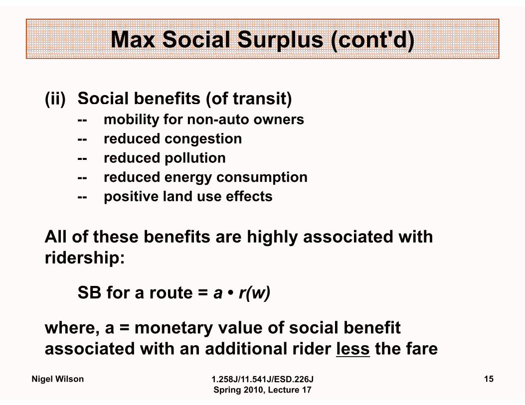
(ii) Social benefits (of transit)(ii) (of transit)-- mobility for non-auto owners-- reduced congestion-- redducedd poll lluti tion-- reduced energy consumption-- ppositive land use effects

All of these benefits are highly associated with id hiridership:

SB for a route = a • r(w)( )

where, a = monetary value of social benefit associated with an additional rider less the fareassociated with an additional rider less the fare


15

We know w

=


We know w = f(h)f(h)

derive the function r(h) from r(w)i.e., r(h) = r(f(h))

(iii)(iii) Total social surplus to maximize: Total social surplus to maximize:

CS + SB =CS + SB

where h* is the headway on route i whose optimal where h is the headway on route i whose optimal value is to be determined (decision variable)


16

Constraints


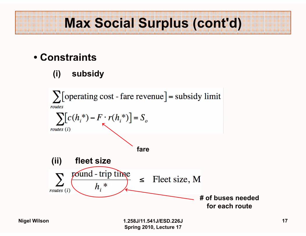
• Constraints (i) subsidy

ffare

(ii) fleet size

# of buses needed ffor eachh routte


17


(iii) Level of service( )

h* < ho

vehicle load < lo

g(h*)

ho, lo = headway and load standards


18

Critical


Critical Assumptions/Limitations:Assumptions/Limitations: • independence across routes

i.e., ridership on a route depends only on the headway of that route BUT, in general, ridership also depends on headways on competing routes and complementary routes (transfers)

• nettwork d k desiign iis nott consid ideredd

Advantages:Advantages: • ridership = f (frequency) • captures trade-offs across routes offs across routescaptures trade • introduces system wide budget constraint



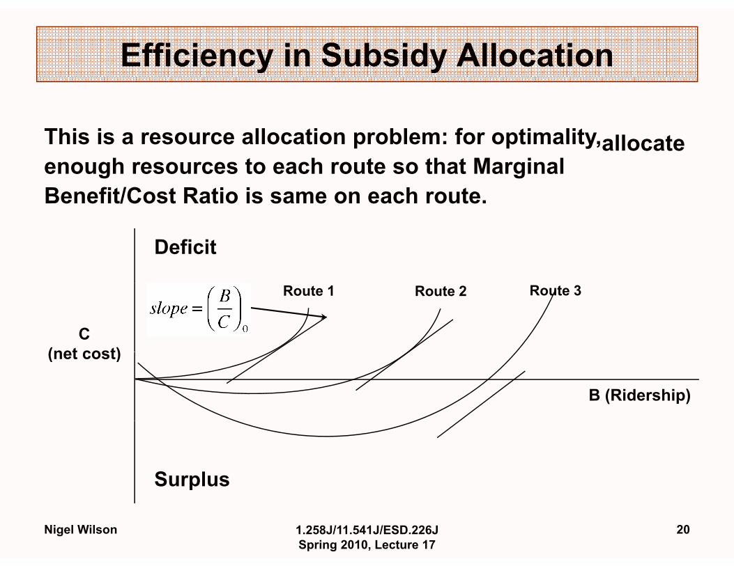
Efficiency in Subsidy Allocation

This is a resource allocation pproblem: for opptimality,y, allocate enough resources to each route so that Marginal Benefit/Cost Ratio is same on each route.

Deficit

C (net cost)

Route 1 Route 2 Route 3

B (Ridership)

(net cost)

Surplus


p

Conclusions

• sqquare root rule is valid where constraints are not bindingg

• problem can be solved using Lagrangian relaxation and single variable search techniques -- not very complexsingle variable search techniques not very complex

• existing scheduling practice over allocates service to peak and to long, high ridership routespeak and to long, highridership routes

• minimizing wait time assuming fixed demand gives similar solutions to more complex objective and variable demandsolutions to more complex objective and variable demand

• best allocation of resources is quite robust with respect to objectives and parameters assumedobjectives and parameters assumed


21

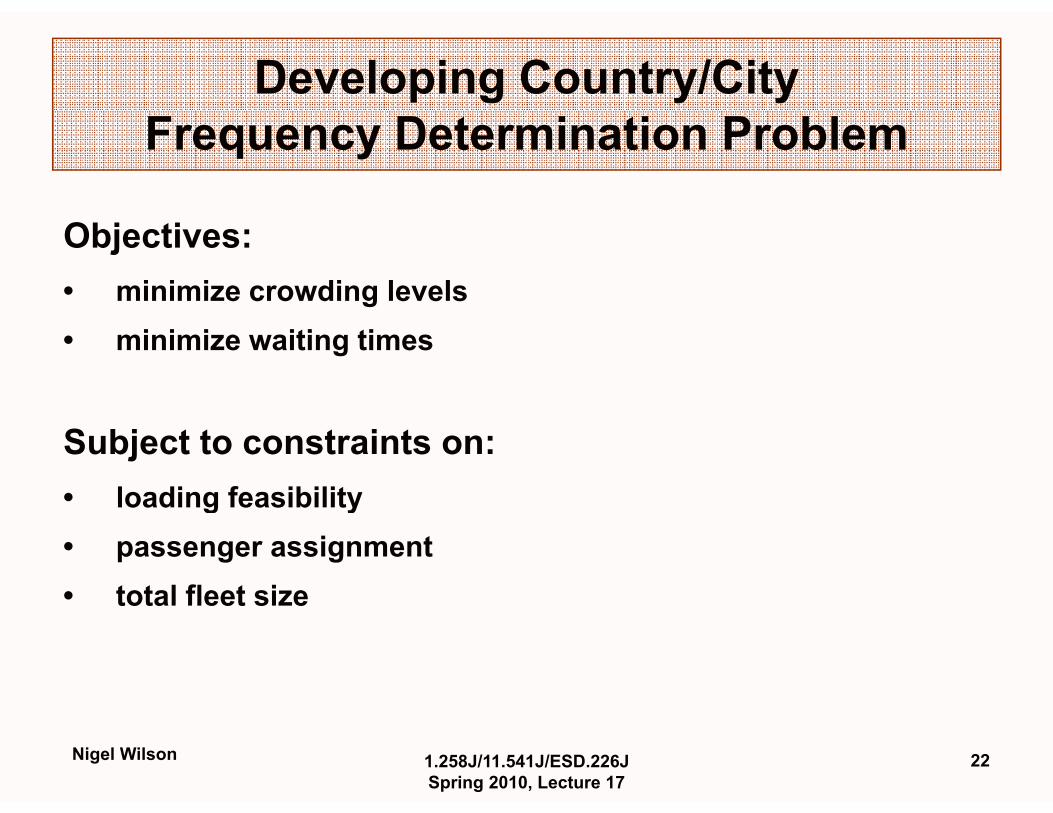
Developing Country/City Frequency Determination Problem

Objectives: • minimize crowding levels • minimize waiting times

Subject to constraints on: • loading feasibilityloading feasibility • passenger assignment • total fleet sizetotal fleet size


t

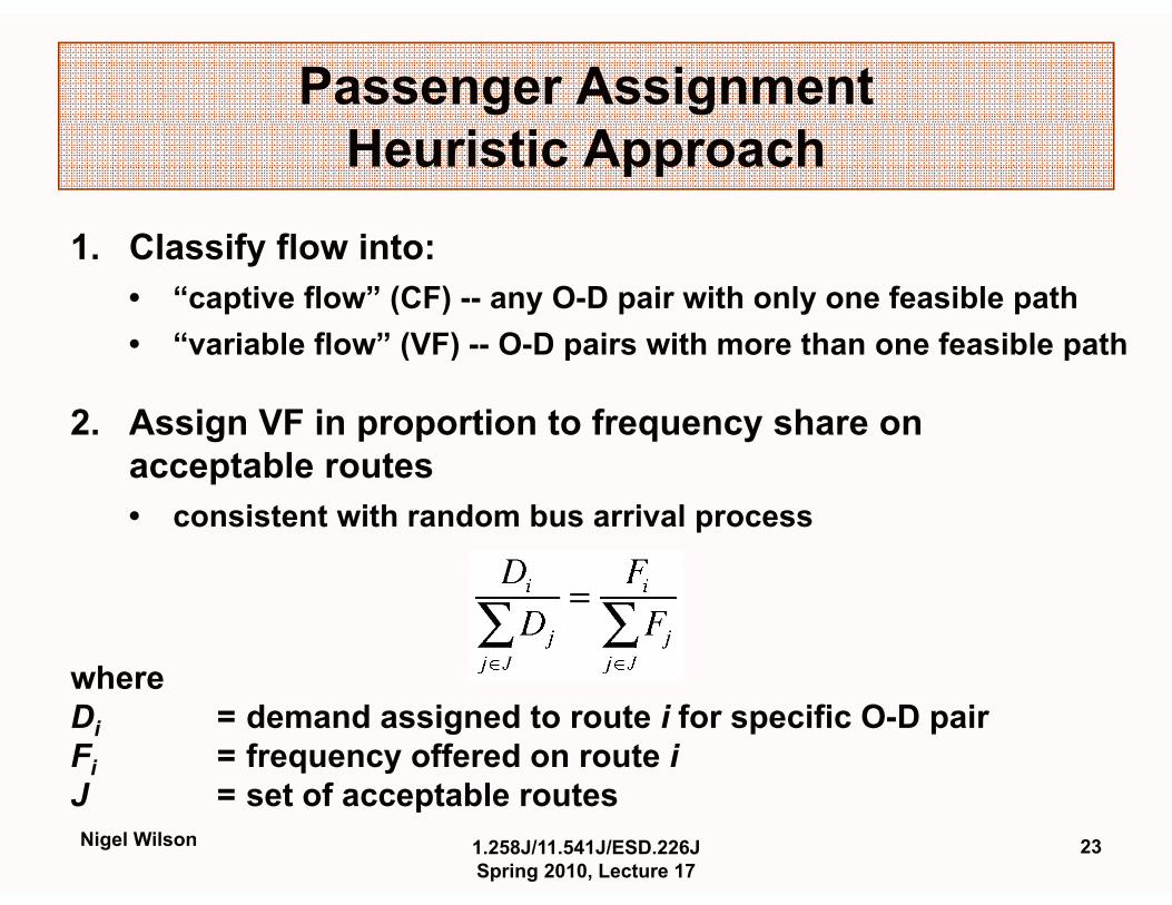
Passenger Assignment Heuristic Approach

1. Classify flow into: • “captive flow” (CF) -- any O-D pair with only one feasible path •• “variable flowvariable flow” (VF) O D pairs with more than one feasible path (VF) -- O-D pairs with more than one feasible path

2. Assign VF in proportion to frequency share on accept bltable routes • consistent with random bus arrival process

wherewhere Di = demand assigned to route i for specific O-D pair Fi = frequency offered on route i J = set off acceptable routes



t

Models

A. Normative Model • “assign” passenger flows to routes with minimum round

trip vehicle time among all acceptable paths • compute frequency and fleet size required on this

assignment basis

B. Descriptive Model • assign passengers to alternative acceptable paths in

proportition to ffrequency shhare iin an ititeratitive process

The difference in the total fleet sizes from the normative and descriptive models indicates the extent of inefficiency resulting from the overlapping route structure.


24

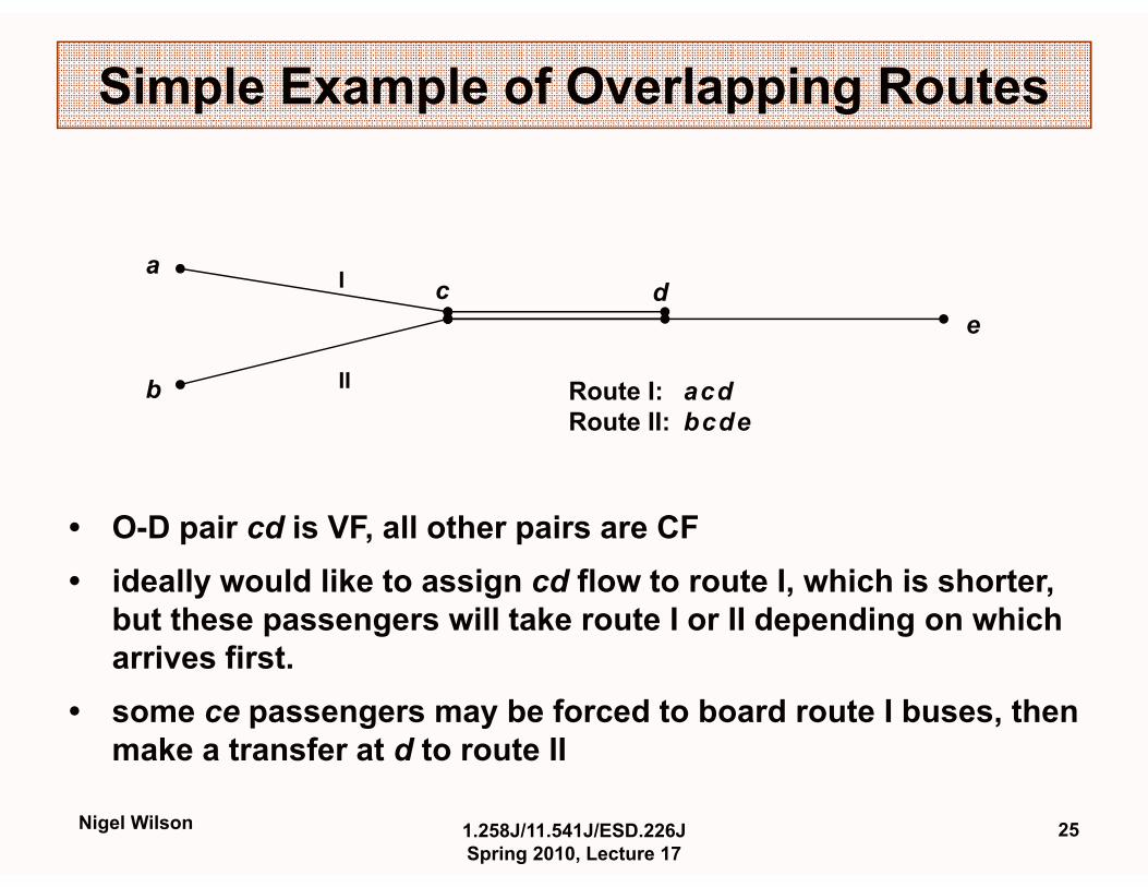
Simple Example of Overlapping Routes

a I c d e

b II Route I: acd Route II: bcde

• O-D pair cd is VF, all other pairs are CF • ideally would like to assign cd flow to route I, which is shorter,

but these passengers will take route I or II depending on which arrives firstarrives first.

• some ce passengers may be forced to board route I buses, then make a transfer at d to route II


25

MIT OpenCourseWarehttp://ocw.mit.edu

1.258J / 11.541J / ESD.226J Public Transportation SystemsSpring 2010

For information about citing these materials or our Terms of Use, visit: http://ocw.mit.edu/terms.

http://ocw.mit.edu

http://ocw.mit.edu/terms

1.258J Lecture 17, Frequency determination

Documents

Transcript of 1.258J Lecture 17, Frequency determination