FORCES. 9/7/2006ISP 209 - 2B2 Which vehicle exerts a greater force ― the tow truck or the car?

12220 Greenland Place Richmond, B.C. V6V-2B2 April 11, 2005 Dr. David Michelson, Assistant Professor University of British Columbia Department of Electrical and Computer Engineering 2356 Main Mall Vancouver, B.C. V6T-1Z4 Re: EECE 496 Final Report: Measurement-based Modeling of Propagation in
Vehicular Environments – Part III. Results and Data Analysis
Dear Dr. Michelson: Enclosed you will find my EECE496 report entitled “Measurement-based Modeling of Propagation in Vehicular Environments – Part III. Results and Data Analysis” This report is part III of the final report for the project, “Measurement-based Modeling of Propagation in Vehicular Environments”. There are in total three parts to the final report: “Part I. Overview and Literature Survey”, “Part II. Measurement Methodology and Tool Development” and “Part III. Results and Data Analysis”. Stanley Ho is the main author for part I, Antonio Lau is the main author for part II, and I am the main author for part III. Sincerely, Kelvin Chu Enclosure: EECE 496 Final Report: Measurement-based Modeling of Propagation in Vehicular Environments – Part III. Results and Data Analysis

The University of British Columbia Department of Electrical and Computer Engineering
EECE 496 Engineering Project
DM3: Measurement-based Modeling of Propagation
in Vehicular Environments – Part III. Results and Data Analysis
Kelvin Chu 85266013
Advisors:
Dr. Michelson Nima Mahanfar
Group members:
Stanley Ho Antonio Lau
EECE 496 The University of British Columbia
April 11, 2004

ii
ABSTRACT
Radiowave propagation models are essential to wireless network designs in vehicular
environments. Before a general propagation model can be developed, a large amount of
data should be collected and compared to the hypotheses. Therefore, data reduction
methodologies that allow easy and effective comparisons between our experimental
results and theoretical predictions were developed and reported. Moreover, any
similarities and discrepancies between our results and hypotheses were examined.
Finally, conclusions were drawn regarding the validity of our original hypotheses.
Results showed that S21 parameter generally decreased with distance in a straight-line
fashion with different pathloss coefficients. The pathloss coefficients for Bluetooth
receivers placed at roof height were around 2, signifying the characteristic of free space
propagation that we have predicted. In addition, the hypothesis of higher initial insertion
loss for receiver placed at bumper height than roof height was validated. However, the
pathloss coefficients at bumper height were smaller than what we have expected. Finally,
the coverage when the Bluetooth transmitter was placed near the dome light was found to
have the best coverage around a vehicle.

iii
TABLE OF CONTENTS
Abstract …………………………………………………………………… ii
Table of Contents …………………………………………………………… iii
Glossary …………………………………………………………………… v
List of Abbreviations …………………………………………………………… vi
1.0 Introduction …………………………………………………………… 1
2.0 Raw Data Measurement ………………………………………………… 3
3.0 Data Reduction Methodology ………………………...………………… 8
3.1 S21 vs. Distance Plots (for each transmitter position, angle
and receiver height) …………………………………………….. 8
3.1.1 Data Presentation …………………………………………. 8
3.1.2 Matlab Script Description ………………………………… 9
3.2 S21 vs. Distance Plots (for each transmitter position, angle
and receiver height) …………………………………………….. 11
3.2.1 Data Presentation ………...……………………………11
3.2.2 Matlab Script Description …………………………… 12
3.3 Scatter Plots ………….………………………………………… 13
3.3.1 Data Presentation ………...……………………………13
3.3.2 Matlab Script Description …………………………… 13
4.0 Results ……………. ………………………………………………….. 15
4.1 General Observations from Reduced Data ……………………… 15

iv
4.2 Angular Dependency of the Reduced Data …………………… 17
4.3 Scatter Plot of Neon …………………….……………………… 19
4.4 Scatter Plot of RAV4 ……………………….…………………… 22
4.5 Scatter Plot of Sundance ………………………………………..... 24
5.0 Conclusions ………………………..…………………………………… 28
6.0 References …………………………………………………………… 29
7.0 Appendix …………………………………………………………… 28

v
GLOSSARY
Pathloss: Wave energy loss through propagation.
Vehicular environment: Includes the inside and the area around a vehicle as well as
the radio link between the interiors of two vehicles in a
short distance.
S21 Parameter: Forward transmission coefficients between the incident and
reflected waves.
Vector Network Analyzer: A “stimulus-response” test set that is used to determine the
characteristics of an unknown device or system
Multipath Fading: Signal attenuation due to collisions between signals with
different delay spreads.
Noise floor: The signal strength of all the noise. A signal must be above
the noise floor in order to be distinguishable.

vi
LIST OF ABBREVIATIONS
VNA – Vector Network Analyzer
dB – Decibel
GHz – Gigahertz
RF – Radio Frequency

1
1.0 INTRODUCTION
In the first and second part of this project report, the background and motivations,
anticipated outcomes, research methodology and tool development have been discussed.
The measurement procedure yielded a huge amount of data which must be
reduced before our hypotheses are validated, models developed, and conclusions drawn.
Therefore, part 3 of the report will investigate into the experimental results that we
obtained from our production runs. The objective is to compare these results with our
anticipated outcomes. A strong agreement between the experimental data and our
hypotheses will allow us to develop a Bluetooth propagation model for any automotive
environment. Such a propagation model is an essential tool for wireless network design
in vehicular environments, and it has not been explored in detail previously.
In this report, sample of raw data will first be shown and discussed. Moreover, the
methodology for data reduction is presented followed by sample processed data for
different cases (i.e. Different vehicle types). For brevity, only reduced data that have
significant conclusions are presented. Any discrepancy between our experimental data
and our expected results will be discussed. Finally, several conclusions will be drawn
regarding our original hypotheses.

2
This report is divided into the following primary sections: Raw Measurement Data, Data
Reduction Methodology, Results, Conclusions, References, and Appendix.

3
2.0 RAW MEASUREMENT DATA
From our pre-development and production runs, we have collected a very large amount of
data. To be exact, we have collected 107 and 628 sets of data for pre-development runs
and production runs respectively. In the production runs, we have collected data from
three different vehicles according to the measurement plan specified in part 2 of the
report. The three vehicles were a Neon Sedan, a Rav4 and a Sundance.
Each set of data that we have collected essentially was the frequency response for a
specific position of the Bluetooth transmitter and the Bluetooth receiver. In the vector
network analyzer (VNA), the data was represented by a graph that plots the S21
coefficients with a range of frequency values. S21 coefficients were measured in decibel
(dB), and frequency values were in gigahertz (GHz). The frequency range was set to be
between 2.4GHz and 2.55GHz because we know that the operational frequency for
Bluetooth is around 2.45GHz. Moreover, we have set the VNA to collect 1601 data
points in the frequency range in order to get a more accurate frequency response.
When we saved the data to the floppy disks, the VNA would create a file with an
extension of .dat. This file did not show the plot that we observed from the VNA.
Instead, it was a text file that begins with some texts describing the settings of the VNA.
Some of the settings were the start and stop frequency values, the parameter measured
and the reference plane value. Following the VNA settings, 1601 different frequency

4
values with their corresponding S21 values were listed. A sample of the data file that we
saved is shown in Exhibit 1 in the Appendix. Note that only the first 2 pages of data are
shown.
From Exhibit 1, we can see that there are texts in between the data at the end of each page
of the file. In order to plot the data in Matlab, we need to delete all the text and input
only the 1601 pairs of data points to the program. To do this, one of Dr. Michelson’s
assistants, Chris, has helped us to develop a Matlab function that would extract the
numerical data from the file effectively. This function is named “load_data”, and its
Matlab script is shown in Exhibit 2 in the Appendix.
In this Matlab script, Chris first counted the number of rows for the header, data blocks
and the texts between the data blocks. Using this information, Chris could then skip all
the undesired content in the data file and input all the frequency and S21 values into two
1601x1 matrixes. Since the formats of all data files were exactly the same, this Matlab
function can be used for all data files that we have collected in the production runs. To
use this function, we just have to input the file name that we want to extract the data
from. For example, to extract the data from the “PORT130.dat” file in Exhibit 1, this
command should be input in Matlab:
[freq, mag] = load_data(PORT130.dat)

5
After that, two 1601x1 matrixes, “freq” and “mag”, will be created. “freq” will contain
1601 different frequency values from 2.4GHz to 2,55GHz while “mag” will contain 1601
S21 values in dB. Using the “plot(freq, mag)” Matlab command, a plot of S21 vs.
frequency can be produced, and it is very similar to the plot that we saw in the VNA. A
sample of such a plot for the “PORT130.dat” file is shown below:
Figure 1. Pathloss vs. Frequency Plot for “PORT130.dat”
The peaks and dips in the plot above are the result of interference between multipath
replicas of the original signal that arise from reflections in and around the vehicle.

6
Another interesting fact that we noticed from the plots of frequency responses is that the
frequency response would have more distortion as the receiver moves further away from
the transmitter. The plot above used data of “PORT130.dat”, which represented a
distance of 2 meters between the Bluetooth transmitter and receiver. Another data plot of
S21 vs. frequency is plotted below at a distance of 12 meters from the “PORT134” file:
Figure 2. Pathloss vs. Frequency Plot for “PORT134.dat”
From the plot above, we can notice that there are more fluctuation and distortion for the
S21 values at a distance of 12 meters than at 2 meters. This is due to multipath fading

7
that attenuates and distorts the signal more as the distance increases. Beside the
distortion, we can also notice that the average value of S21 decreases as the distance
increases. However, the questions of how much it decreases as well as how the decrease
relates to different positions and heights of the Bluetooth transmitter and receiver still
remain unanswered. In order to find the answers to the questions and to verify our
hypotheses, an effective way to reduce the data into a format that can be easily analyzed
was developed. In the following section, this methodology of data reduction will be
demonstrated.

8
3.0 DATA REDUCTION METHODOLOGY
3.1 S21 vs. DISTANCE PLOTS (for each transmitter position, angle and receiver height)
3.1.1 DATA PRESENTATION In order to analyze the data that we collected in the production runs effectively, we
organized the data in a special manner. The data was reduced and put into plots that
show the relationship between pathloss (S21) and distance at every angle, transmitter
position and receiver height. In the production runs, our measurements were done at five
different angles, four different transmitter positions and two different receiver heights for
each car. Therefore, there would be a total of 40 plots for each automobile. In addition,
the pathloss values in dB were plotted against log distance. A linear regression line was
also drawn in order to find the pathloss coefficient easily. As discussed earlier in part 1
of the report, the relationship between pathloss and the distance from the RF transmitter
to the receiver is given by:
−=
α
πλR
dBPathloss4
log10)( (1)
Hence, it is clear that the pathloss coefficient α can be found simply by dividing the slope
of the regression line in the graphs by –10. Along with the slope, the y-intercept, which

9
represents the initial insertion loss, was also shown at the upper right corner for each
graph. Moreover, the range of values in the pathloss axis was set to be consistent across
all plots to allow easier comparison.
3.1.2 MATLAB SCRIPT DESCRIPTION
To reduce the data in the way described above, we have developed a Matlab script. This
script is shown in Exhibit 3 in the Appendix. Note that only one part of the script is
shown, and this part would only yield one plot out of the 40 plots that we obtained. In
this Matlab script, we first defined the different distance values that we did the
measurements at. Since there were some points that we could not do the measurements
because the vehicle body was in the way, we have defined 3 different vectors of
distances. One vector contained four terms from a distance of 4m to 12m while the
second one contained five terms from 2m to 12m. The last vector contained all six terms
from 1m to 12m. Therefore, different vectors would be used according to the data
collected. After defining the distance vectors, we found the logarithmic values for the
distances because we wanted to plot S21 in dB with log distance values. After that, we
used the “load_data” function to extract the numerical data from the files that had the
same angle, transmitter position, and receiver height. In this case, the transmitter position
was at the dashboard, and the receiver was at bumper height. Moreover, the angle was at
zero degree, which corresponded to the axis pointing towards the back of the car. Under
such conditions, we only did 4 measurements along the axis. Therefore, we only loaded

10
4 files using the “load_data” function. Then, we used the “mean” function to find the
linear average of S21 values for each distance value. Therefore, a vector of 4 different
means of S21 was then created. We also used the “std” function to find the standard
deviations for each distance value, but we did not show them in the plots. Using the
“regress” function, the slope and intercept of the regression line were obtained. For this
function, we should input the vertical and horizontal parameters that we want to draw the
regression line with, which were the S21 mean vector and the log distance vector. We
then input the S21 mean vector and the log distance vector to the “plot” function, and the
original data were plotted. We also used the “axis” function to make sure that the vertical
axis was consistent throughout all the 40 plots. Finally, we used the obtained slope and
intercept to plot the regression line using the “plot” command. We also used the color of
red for the regression line, and we also have put legend that shows the slope and intercept
of the regression line at the upper right corner of each plot. Here is an example of the
plot created by the Matlab script in Exhibit 3:

11
Figure 3. Pathloss vs. Log Distance Plot for Exhibit 3
Using similar Matlab code with different log distance vectors and data files, all 40 plots
were created.
3.2 S21 vs. DISTANCE PLOTS (for each transmitter position and receiver height)
3.2.1 DATA PRESENTATION After obtaining the 40 plots of pathloss vs. log distance, the data was further reduced to
show pathloss vs. log distance without the angle factor. In this presentation, the pathloss
values at different angles for each distance, transmitter position and height were
averaged. Therefore, there would be a total of 8 plots for 4 different transmitter positions

12
and 2 different heights for each vehicle. The format of these plots was the same as the
previous plots which showed the slopes and intercepts of the regression line.
3.2.2 MATLAB SCRIPT DESCRIPTION
The Matlab code for one of these 8 plots is shown in Exhibit 4 in the Appendix. This
code was very similar to the previous one in Exhibit 3. The only difference was that it
had to take the linear average of S21 at the five different angles for each particular
distance, transmitter position, and receiver height at the beginning of the code. After that,
the rest of the code was the same except different parameters were used. The 8 different
plots were created for each vehicle using similar code with different parameters. Here is
the plot that was created with the code in Exhibit 4:

13
Figure 4. Pathloss vs. Log Distance Plot for Exhibit 4
3.3 SCATTER PLOTS
3.3.1 DATA PRESENTATION
The main purpose of our data analysis is to identify trends in the slopes and intercepts of
our graphs, so that we can prove or disprove our hypotheses. Therefore, it is very
convenient if all the slopes and intercepts are shown in one graph. Using the 8 plots
above, the values of slopes were plotted against their respective values of intercepts for
each transmitter position and height in a scatter plot. This scatter plot had 8 data points,
and the 4 different transmitter positions were represented by 4 unique symbols, “x” for
dashboard, “+” for gearbox, “*” for dome light and “∆” for under dash. On the other
hand, the 2 different heights were represented by two different colors, blue for bumper
height (0.5m) and black for roof height (1.5m).
3.3.2 MATLAB SCRIPT DESCRIPTION
The Matlab code for this scatter plot is shown in Exhibit 5 in the Appendix. This code
simply used the slopes and intercepts obtained in the code of Exhibit 4 and plotted them
all in one graph. Therefore, 8 data points were plotted with different symbols and colors

14
in the plot representing 4 different transmitter positions and 2 different receiver heights.
The scatter plot created by the code in Exhibit 5 is shown here:
Figure 5. Scatter Plot of Slopes and intercepts for Exhibit 5

15
4.0 RESULTS
All of the processed data plots for the three cars that we measured in the production runs
are shown in the Appendix (refer to Exhibit 10). This section will only show some
significant findings and thus, only some plots are used for illustration.
4.1 GENERAL OBSERVATIONS from REDUCED DATA
Our first observation was that the values of the slopes in the reduced data graphs were
generally negative (refer to Exhibit 6 in the Appendix). Moreover, many graphs showed
that the pathloss values decline in a straight-line fashion. As an example, one of the
pathloss vs. distance plots is shown below:

16
Figure 6. Pathloss vs. Log Distance Plot (TX at Gearbox, Rx at Roof Height, Car =
Sundance)
The original data points can be seen to be very close to the values of its linear regression
line, meaning that the pathloss values were declining in a straight-line manner. Although
most of the slopes were negative, indicating that S21 generally decreased with distance,
there were some specific instances where S21 actually increased with distance. For
example,
Figure 7. Pathloss vs. Log Distance Plot (TX at Dome Light, Rx at Roof Height, Angle
=67.5, Car = Sundance)
In this plot, we can see that S21 increased initially and gradually declined, resulting an
overall negative slope. This behavior might be due to the lack of line-of-sight between

17
the Bluetooth transmitter and receiver when the receiver was placed very close to the
vehicle; as a result the vehicle body blocked the direct path. As the receiver was moved
further away from the vehicle, line-of-sight appeared again causing S21 to increase
temporarily. Also, this behavior might be due to the large RF penetration into the
metallic material of the automobile body, which significantly decreased the level of S21
when the receiver was close to the vehicle.
From Exhibit 6 in the Appendix, two plots out of a total of 160 pathloss vs. distance plots
actually had positive slopes but the slopes were both close to zero. These 2 positive
slopes occurred at plots with transmitter placed near the dome light in the Neon with an
angle of zero, meaning that the measurements were done on the axis pointing to the back
of the car. Both plots only contained 4 data points since measurements at a distance of
1m and 2m were not made due to the obstruction from the vehicle body. Therefore, the
signals might have already reached the noise floor when the measurements started at the
distance of 4, and a little bit of fluctuation in the signal could result in a positive slope.
For more accurate results, more measurements should be taken at a smaller distance than
4m to compensate for any fluctuations around the noise floor after 4m. However, since
there were only 2 positive slope values and the accuracy of the data was dubious, we still
concluded that S21 decreased with distance around an automobile.
4.2 ANGULAR DEPENDENCY of the REDUCED DATA

18
After observing that S21 generally decreased with distance, we also looked into the
angular dependency of the pathloss vs. distance plots. From Exhibit 6 in the Appendix,
we noticed that the intercept values were fairly close together for measurements at
different angles with same transmitter location and receiver height in the same vehicle.
For example, the largest difference in the intercept values for measurements conducted in
the Rav4 at a transmitter location near dome light and the receiver at bumper height was
only around 5dB. Therefore, initial insertion losses were quite consistent for different
angles. However, we noticed more differences in the values of slope for different angles.
At some instances, the largest difference between the values of slope was around 20 for
measurements at different angles with same transmitter location and same receiver height
in the same car. This was equivalent to a difference of 2 in pathloss coefficient. This was
not expected in our hypotheses since our hypotheses predicted that the pathloss
coefficients would be affected mainly by different receiver heights. With further
investigation, we found that the discrepancies were sometimes due to the inaccuracy of
measurements conducted at zero degree since these values were generally quite different
from the values at other angles. The inaccuracy was caused by inadequate measurements
that were discussed before. For the measurements conducted in the Neon with a
transmitter location near dome light and receiver at roof height, the slope at zero degree
was 0.713 and the slopes at other angles were all between 10 and 20. If we ignore the
values of slope at zero degree in some cases, the differences in the slopes were within
reasonable range. Moreover, there was not a clear trend for angular dependency since we
could not find any similar trends even when we compared the pathloss behavior under

19
same conditions in the two sedans, the Neon and the Sundance. Therefore, we insisted
that pathloss behavior did not depend on angles, but rather on the structures of the
vehicles. Different structures include different placements and sizes of doors, passenger
seats and windows. A slight change in the structure from the Neon to the Sundance
would yield different angular pathloss behaviors. Therefore, more data should be
collected in order to incorporate the angular factor in a general propagation model for a
certain vehicle class.
Now, we have proven that S21 decreased with distance, and the relationship between
pathloss and distance was generally not angular dependent; we were justified to take the
linear averages for slope and intercept values at different angles to create the scatter plots.
In the following 3 sections, we will investigate into the pathloss coefficient and initial
insertion loss for each vehicle by examining the slopes and intercepts respectively from
the scatter plots without the angular factor.
4.3 SCATTER PLOT of NEON
For the first vehicle that we measured, the Neon, here is the scatter plot of the slopes and
intercepts for each transmitter position and receiver height (refer to Exhibit 7 in the
Appendix for exact values of slope and intercept):

20
Figure 8. Slope vs. Intercept Scatter Plot (Car = Neon)
From this plot, we can observe that for all of the transmitter positions at roof height, the
values of the slope were between -15 and -25. This corresponds to pathloss coefficients
from 1.5 to 2.5. This was close to our hypothesis, which we expected the pathloss
coefficient to be 2 for receiver at roof height since we have assumed free space
propagation at this height. However, when the receiver was at bumper height, we
expected the coefficient to be 4 but all of the experimental values were nowhere near that
value. In fact, the experimental values for pathloss coefficient at bumper height were
generally smaller than the ones at roof height. The smallest pathloss coefficient, which
was around 0.73, occurs when the transmitter was placed at the dome light and the
receiver was at bumper height. This experimental result contradicted our hypothesis,

21
which predicted that the pathloss coefficient would get closer to 4 as the receiver became
closer to the ground.
For the other hypothesis, we have predicted that the initial insertion loss should be less
for the receiver at roof height than at bumper height. From our experimental data, we
observed that the intercepts at roof height were generally higher than the intercepts at
bumper height. Therefore, the experimental results support our hypothesis.
In addition, we also predicted that the coverage would be best with the lowest initial
insertion loss when the transmitter is placed near the dome light. This was not true for
the Neon, as the intercepts for transmitter near dome light at both bumper height and roof
height were relatively low compared to other transmitter positions. For the 4 different
transmitter positions at roof height, the highest initial insertion loss actually occurred
when the transmitter was placed near the dome light. Surprisingly, at both heights, the
initial insertion loss was minimal when the transmitter was placed at the dashboard.
Although there was a low initial insertion loss for transmitter placed at the dashboard, it
was not necessary for this position to provide the best coverage outside a vehicle. It is
because the pathloss coefficients for transmitter placed at dashboard were also the
greatest among other transmitter positions. This means that S21 would decline most
rapidly with distance when the transmitter was placed at the dashboard. Although the
initial insertion loss for transmitter placed at dome light was large, its pathloss
coefficients were smallest among the others. In fact, the S21 value for transmitters at

22
dome light at a distance of 12 meters was around –70 dB while the S21 values for other
transmitter positions were all around –75 dB. For transmitters placed under dash and at
gearbox, they had higher initial insertion loss than transmitter placed at dashboard, and
they also had a higher pathloss coefficient than the transmitter near dome light.
Therefore, their coverage was even worse.
4.4 SCATTER PLOT of RAV4
The second vehicle that we measured was the Rav4. Since the structure of a Rav4 is
completely different than the Neon, we expect to find some differences in the collected
data. Here is the scatter plot of the slopes and intercepts for each transmitter position and
receiver height (refer to Exhibit 8 in the Appendix for exact values of slope and
intercept):

23
Figure 9. Slope vs. Intercept Scatter Plot (Car = RAV4)
From this plot, we observed some similarities with the Neon. For example, we noticed
that the slopes were generally steeper for transmitters at roof height than at bumper
height. The scatter plot of the Neon also showed similar behavior. This illustrated that
the pathloss coefficients at roof height were greater than those at bumper height, and this
contradicted our hypothesis. The only thing that met our predictions was that the
pathloss coefficients at roof height were around 2, which represents the pathloss
coefficient in free space. On the other hand, the pathloss coefficients at bumper height
were again nowhere near its predicted value of 4.

24
Beside the pathloss coefficients, the Rav4 showed similar behavior with the Neon as the
initial insertion loss at bumper height were generally greater than the loss at roof height.
This experimental result coincides with our prediction.
For transmitter at dome light in the Rav4, the pathloss coefficient was small while the
initial insertion loss was large compared to other transmitter positions. This behavior is
consistent with the results for the Neon. For transmitter at dashboard and under dash,
strange behavior was observed for the Rav4. When the dashboard transmitter was
coupled with a receiver at roof height, it resulted in very low initial insertion loss and
very high pathloss coefficient. However, when the dashboard transmitter was coupled
with a receiver at bumper height, it resulted in a very low pathloss coefficient and a very
high insertion loss. In addition, the transmitter under dash displayed a completely reverse
behavior to the dashboard transmitter. For the gearbox transmitter, the result showed that
it had the second lowest initial insertion loss and the second highest pathloss coefficient
for both receiver heights.
4.5 SCATTER PLOT of SUNDANCE
The last vehicle that we measured was a sedan, the Sundance. Since the structure of the
Sundance is very similar to the Neon, we expect to find many similarities in the collected
data. Here is the scatter plot of the slopes and intercepts for each transmitter position and

25
receiver height (refer to Exhibit 9 in the Appendix for exact values of slope and
intercept):
Figure 10. Slope vs. Intercept Scatter Plot (Car = Sundance)
From this scatter plot, we again noticed that the pathloss coefficients were higher and the
initial insertion losses were lower at roof height than at bumper height. This behavior is
consistent for all 3 vehicles tested. Another observation of the scatter plot w that the data
points were closer together both vertically and horizontally when compared to the two
other plots for the other cars. The pathloss coefficients at bumper height were again not
close to what we have predicted. The low values of pathloss coefficients might be due to
the high initial insertion loss at bumper height, and S21 was hitting the noise floor too
rapidly. This would then result in a flat regression line. Since the values of initial

26
insertion loss when the receiver was at bumper height were around –60dB, it was
impossible to result in a slope of –40 since the noise floor was around –80dB. For
example,
Figure 11. Pathloss vs. Log Distance Plot (TX at Gearbox, Rx at Bumper Height, Car =
Sundance)
In this plot, we can notice that S21 decreased rapidly at first and settled for a less decline
when it reached the noise floor. For a more accurate estimate of pathloss coefficient at
bumper height, we should use the first few distance points only to plot the regression line.
However, the exact number of points to be used in different situations is difficult to be
determined.

27
For transmitter at dome light in the Sundance, it had relatively low pathloss coefficients
for both bumper and roof height, similar to the results obtained from the other two cars.
Moreover, it had a high insertion loss when the receiver was placed at roof height just
like the other 2 previous cases. However, the only difference occurred at bumper height
while it resulted a relatively low insertion loss.
The initial insertion loss was minimal when the transmitter was placed under dash for the
Sundance. In addition, the pathloss coefficient was at its maximum at this transmitter
position. Compared to the data for the Neon, similar behavior was found with the
transmitter at the dashboard of the Neon. With further investigation, we also noticed that
the behavior for under dash transmitter in the Neon is similar to the behavior for
transmitter at the dashboard in the Sundance. This behavior swap might be due to the
difference in mounting angles when we did the measurements. For example, when we
mounted the transmitting antenna at the dashboard, we might have aimed the antenna
upward for the Neon but aimed the antenna downward for the Sundance. As for the
transmitter at gearbox, it had relatively high pathloss coefficients and medium initial
insertion loss.

28
5.0 CONCLUSIONS
This report investigated into the experimental results and compared them to our original
hypotheses. The hypothesis that S21 would decrease with distance in a straight-line
manner was validated. In addition, the relationship between pathloss and distance did not
depend on angles, but rather on the structures of the vehicles. The experimental results
also proved that the initial insertion loss was higher at bumper height than at roof height.
Moreover, it was also shown that propagation at roof height could be assumed to be free
space as the pathloss coefficients were all around the value of 2. However, the measured
pathloss coefficients for receivers placed at bumper height were nowhere near what we
have expected. For transmitters at different positions, transmitter near the dome light
generally had a high initial insertion loss, but it was offset by a very low pathloss
coefficient. Therefore, the coverage of the transmitter at dome light was pretty good.
The coverage of the transmitter placed on and under the dashboard was similar. It is
characterized by low initial insertion loss and high pathloss coefficient. Finally, the
coverage of the transmitter at gearbox was generally the worst among the four.

29
6.0 REFERENCES
[1] D. Michelson, “Introduction to Vector Network Analyzers,” class notes for EECE 483 – Antennas and Propagation, Department of Electrical Engineering, University of British Columbia, Fall 2004.

30
7.0 APPENDIX
Exhibit 1. Sample raw data file (PORT130.dat)
##3���������������������������������������������������������������������������������������������������������������������������������������������������������������������������������������������������������������������������������������������������������� ##2�������������������� 37225A ##1�������������������� MODEL: DATE: Page 1 DEVICE ID: OPERATOR: START: 2.400000000 GHz GATE START: - ERROR CORR: 12-TERM STOP: 2.550000000 GHz GATE STOP: - AVERAGING: 1 PT STEP: 0.000093750 GHz GATE: - IF BNDWDTH: 1 KHz WINDOW: - ---CH1--- PARAMETER: -S21- NORMALIZATION: OFF REFERENCE PLANE: 11.3386cm SMOOTHING: 0.0 PERCENT DELAY APERTURE: - MARKERS: MKR FREQ MAGNITUDE # GHz dB FREQUENCY POINTS: PNT FREQ MAGNITUDE # GHz dB

31
1 2.400000000 -48.417 2 2.400093750 -48.324 3 2.400187500 -48.591 4 2.400281250 -48.513 5 2.400375000 -48.597 6 2.400468750 -48.661 7 2.400562500 -48.811 8 2.400656250 -48.668 9 2.400750000 -48.770 10 2.400843750 -49.251 11 2.400937500 -49.000 12 2.401031250 -49.187 13 2.401125000 -49.202 14 2.401218750 -49.310 15 2.401312500 -49.578 16 2.401406250 -50.146 17 2.401500000 -49.955 18 2.401593750 -50.014 19 2.401687500 -50.168 20 2.401781250 -50.026 21 2.401875000 -50.296 22 2.401968750 -50.225 23 2.402062500 -50.395 24 2.402156250 -50.483 25 2.402250000 -50.678 26 2.402343750 -51.493 MODEL: DATE: Page 2 DEVICE ID: OPERATOR: ---CH1--- FREQUENCY POINTS: PNT FREQ MAGNITUDE # GHz dB 27 2.402437500 -51.107 28 2.402531250 -50.730 29 2.402625000 -51.567 30 2.402718750 -51.490 31 2.402812500 -51.473 32 2.402906250 -51.819 33 2.403000000 -51.811

32
34 2.403093750 -52.358 35 2.403187500 -52.172 36 2.403281250 -51.673 37 2.403375000 -52.611 38 2.403468750 -52.005 39 2.403562500 -51.977 40 2.403656250 -52.478 41 2.403750000 -52.397 42 2.403843750 -52.528 43 2.403937500 -52.541 44 2.404031250 -53.095 45 2.404125000 -53.167 46 2.404218750 -52.885 47 2.404312500 -52.938 48 2.404406250 -53.061 49 2.404500000 -52.822 50 2.404593750 -52.944 51 2.404687500 -53.506 52 2.404781250 -53.645 53 2.404875000 -53.839 54 2.404968750 -53.854 55 2.405062500 -54.308 56 2.405156250 -54.077 57 2.405250000 -54.006 58 2.405343750 -54.699 59 2.405437500 -53.887 60 2.405531250 -54.155 61 2.405625000 -54.815 62 2.405718750 -53.905 63 2.405812500 -54.613 64 2.405906250 -54.767 65 2.406000000 -54.765 66 2.406093750 -54.554 67 2.406187500 -54.470 68 2.406281250 -54.692 69 2.406375000 -54.402 70 2.406468750 -55.977 71 2.406562500 -55.142 72 2.406656250 -56.149 73 2.406750000 -54.763

33
Exhibit 2. Matlab Script for the function “load_data”
function [freq, mag] = load_data(file_name)
% % file_name is a string contain the data file name i.e. 'PRE1.dat' % num_points = 1600; header_size = 33; block_size1 = 26; block_size2 = 47; block_size3 = 24; freq = zeros(num_points,1); mag = zeros(num_points,1); num_data_set = 33; %------------------------------------------------------------ % open data file fid = fopen(file_name); % read past header for m=1:header_size fgetl(fid); end %read first data block tmp =fscanf(fid,'%i %f %f',[3,block_size1]); %skip over header for k=1:11 fgetl(fid); end %load variable for k=1:block_size1 freq(k) = tmp(2,k); mag(k) = tmp(3,k); end for m=1:num_data_set %read data block tmp =fscanf(fid,'%i %f %f',[3,block_size2]); %skip over header

34
for k=1:11 fgetl(fid); end %load variable for k=1:block_size2 freq((m-1)*block_size2+block_size1+k) = tmp(2,k); mag((m-1)*block_size2+block_size1+k) = tmp(3,k); end end %read last data block tmp =fscanf(fid,'%i %f %f',[3,block_size3]); %load variable for k=1:block_size3 freq(num_data_set*block_size2+block_size1+k) = tmp(2,k); mag(num_data_set*block_size2+block_size1+k) = tmp(3,k); end % close data file fclose(fid);
Exhibit 3. Matlab Script for Plotting S21 vs. Distance Graphs at one Specific Transmitter
Position, Angle and Receiver Height
%distances used for plotting distance4 = [4,6,8,12]; logdistance4 = log10(distance4); distance5 = [2,4,6,8,12]; logdistance5 = log10(distance5); distance6 = [1,2,4,6,8,12]; logdistance6 = log10(distance6); x4 = [logdistance4',ones(4,1)]; x5 = [logdistance5',ones(5,1)]; x6 = [logdistance6',ones(6,1)]; %Car = Neon Sedan %Tx at Dashboard, Bumper Height, Angle = 0

35
%obtaining the variable [fd3, s21neond3] = load_data('prod1.dat'); [fd4, s21neond4] = load_data('prod2.dat'); [fd5, s21neond5] = load_data('prod3.dat'); [fd6, s21neond6] = load_data('prod4.dat'); %calculate the mean s21neond3_mean = mean(s21neond3); s21neond4_mean = mean(s21neond4); s21neond5_mean = mean(s21neond5); s21neond6_mean = mean(s21neond6); %calculate the standard deviation s21neond3_std = std(s21neond3); s21neond4_std = std(s21neond4); s21neond5_std = std(s21neond5); s21neond6_std = std(s21neond6); s21neon_dash_bumper_0 = [s21neond3_mean, s21neond4_mean, s21neond5_mean, s21neond6_mean];
%calculate the slope and intercept using linear regression bneon_dash_bumper_0 = regress(s21neon_dash_bumper_0', x4); %plotting the data plot(logdistance4, s21neon_dash_bumper_0); axis([0 1.1 -85 -40]); hold on; %plotting the regression line plot(logdistance4, x4*bneon_dash_bumper_0, 'r'); legend('Data',sprintf('Linear Regression, Slope = %5.3f', bneon_dash_bumper_0(1,1)), sprintf('Intercept = %5.3f', bneon_dash_bumper_0(2,1))); xlabel('Log distance (m)'); ylabel('pathloss (dB)'); title('Pathloss vs logdistance with Tx on the Dashboard, Rx at Bumper Height, Angle = 0, Car = Neon Sedan'); pause; Exhibit 4. Matlab Script for Plotting S21 vs. Distance Graphs at one Specific Transmitter
Position, and Receiver Height

36
%Part 2///////////////////////////////////////////////////////////////////////////////////////////////////// %avg pathloss vs distance with tx at dashboard, rx at bumper height s21neon_dash_bumper = [zeros(1,2), s21neon_dash_bumper_0] + [zeros(1,2), s21neon_dash_bumper_225] + [zeros(1,1), s21neon_dash_bumper_45] + s21neon_dash_bumper_675 + s21neon_dash_bumper_90; s21neon_dash_bumper = [s21neon_dash_bumper(1,1)./2, s21neon_dash_bumper(1,2)./3, s21neon_dash_bumper(1,3)./5, s21neon_dash_bumper(1,4)./5, s21neon_dash_bumper(1,5)./5, s21neon_dash_bumper(1,6)./5]; bneon_dash_bumper = regress(s21neon_dash_bumper', x6); figure; plot(logdistance6, s21neon_dash_bumper); axis([0 1.1 -85 -40]); hold on; plot(logdistance6, x6*bneon_dash_bumper, 'r'); legend('Data',sprintf('Linear Regression, Slope = %5.3f', bneon_dash_bumper(1,1)), sprintf('Intercept = %5.3f', bneon_dash_bumper(2,1))); xlabel('Log distance (m)'); ylabel('pathloss (dB)'); title('Pathloss vs Log distance with Tx on the Dashboard, Rx at Bumper Height, Car = Neon Sedan'); pause; Exhibit 5. Matlab Script for Scatter Plot for One Vehicle %Part 3////////////////////////////////////////////////////////////////////////////////////////////// %Slope verse Intercept plot(bneon_dash_bumper(2,1), bneon_dash_bumper(1,1), 'bx'); hold on; axis([-70 -40 -30 -5]); hold on; plot(bneon_dash_Roof(2,1), bneon_dash_Roof(1,1), 'kx'); plot(bneon_Gearbox_bumper(2,1), bneon_Gearbox_bumper(1,1), 'b+'); plot(bneon_Gearbox_Roof(2,1), bneon_Gearbox_Roof(1,1), 'k+'); plot(bneon_Domelight_bumper(2,1), bneon_Domelight_bumper(1,1), 'b*'); plot(bneon_Domelight_Roof(2,1), bneon_Domelight_Roof(1,1), 'k*'); plot(bneon_Underdash_bumper(2,1), bneon_Underdash_bumper(1,1), 'b^'); plot(bneon_Underdash_Roof(2,1), bneon_Underdash_Roof(1,1), 'k^'); text(-58, -6, sprintf('x = Dashboard, + = Gearbox')); text(-58, -7, sprintf('* = Domelight, ^ = Underdash')); text(-58, -8, sprintf('blue -> rx at bumper, black -> rx at roof')); xlabel('Intercept');

37
ylabel('Slope'); title('Slope vs Intercept of Pathloss vs Log Distance, Car = Neon Sedan'); pause; close all; Exhibit 6. Tables of Slopes and Intercepts in Pathloss vs. Distances Plots for Each Transmitter Position, Receiver Height, Angle, and Vehicle RX at Bumper Height, Car = Neon Angles (Degrees)
TX at Dashboard TX at Gearbox TX at Dome Light
TX at Under Dash
Slope Intercept Slope Intercept Slope Intercept Slope Intercept0 -16.594 -58.879 -4.956 -69.621 0.449 -64.348 -16.594 -58.879 22.5 -21.950 -52.776 -15.199 -62.745 -12.431 -58.728 -8.732 -70.210 45 -13.701 -57.060 -5.336 -68.637 -22.369 -50.461 -20.526 -56.563 67.5 -13.527 -57.430 -5.851 -64.209 -4.338 -61.706 -18.814 -60.353 90 -28.994 -47.442 -11.695 -62.488 -9.157 -58.867 -13.060 -64.383 RX at Roof Height, Car = Neon Angles (Degrees)
TX at Dashboard TX at Gearbox TX at Dome Light
TX at Under Dash
Slope Intercept Slope Intercept Slope Intercept Slope Intercept0 -35.881 -34.702 -16.437 -54.389 0.713 -64.050 -26.563 -45.557 22.5 -32.130 -41.706 -15.926 -60.377 -15.475 -53.356 -18.783 -55.419 45 -31.145 -40.107 -16.573 -55.668 -19.877 -49.081 -21.288 -49.273 67.5 -24.688 -46.218 -21.317 -51.766 -11.615 -56.166 -22.626 -51.751 90 -27.792 -47.606 -21.842 -51.483 -21.569 -50.548 -24.042 -53.634 RX at Bumper Height, Car = Rav4 Angles (Degrees)
TX at Dashboard TX at Gearbox TX at Dome Light
TX at Under Dash
Slope Intercept Slope Intercept Slope Intercept Slope Intercept0 -0.990 -68.146 -21.311 -51.190 -2.704 -64.135 -0.990 -68.146 22.5 -1.985 -67.054 -3.615 -66.869 -9.291 -59.774 -9.213 -63.789 45 -8.281 -60.690 -13.479 -55.881 -7.300 -61.183 -2.461 -62.897 67.5 -7.625 -61.822 -9.567 -57.516 -7.409 -58.962 -13.265 -51.893 90 -3.859 -65.332 -9.826 -55.828 -10.048 -59.922 -12.893 -56.634

38
RX at Roof Height, Car = Rav4 Angles (Degrees)
TX at Dashboard TX at Gearbox TX at Dome Light
TX at Under Dash
Slope Intercept Slope Intercept Slope Intercept Slope Intercept0 -21.313 -46.647 -24.965 -39.252 -14.047 -55.903 -31.520 -43.680 22.5 -17.706 -51.650 -18.488 -48.788 -27.561 -43.882 -23.506 -45.292 45 -22.205 -42.318 -24.227 -45.094 -10.183 -56.890 -22.603 -45.581 67.5 -25.588 -44.033 -27.463 -40.518 -19.537 -49.756 -21.543 -49.497 90 -26.598 -43.095 -24.554 -43.285 -20.089 -51.833 -15.654 -55.376 RX at Bumper Height, Car = Sundance Angles (Degrees)
TX at Dashboard TX at Gearbox TX at Dome Light
TX at Under Dash
Slope Intercept Slope Intercept Slope Intercept Slope Intercept0 -1.215 -71.623 -9.129 -65.581 -16.535 -58.485 -1.215 -71.623 22.5 -12.547 -62.446 -10.242 -67.007 -5.158 -64.162 -12.379 -60.918 45 -14.025 -60.924 -8.379 -65.678 -12.951 -58.415 -9.809 -57.878 67.5 -6.806 -65.763 -12.176 -59.952 -12.664 -57.539 -9.980 -57.783 90 -10.822 -63.808 -12.137 -61.184 -14.856 -56.233 -21.018 -52.935 RX at Roof Height, Car = Sundance Angles (Degrees)
TX at Dashboard TX at Gearbox TX at Dome Light
TX at Under Dash
Slope Intercept Slope Intercept Slope Intercept Slope Intercept0 -5.520 -67.188 -23.959 -51.180 -14.073 -57.641 -27.294 -47.811 22.5 -10.595 -61.905 -16.178 -55.126 -9.840 -56.124 -26.765 -47.295 45 -25.757 -49.176 -18.733 -53.539 -9.762 -59.348 -24.631 -47.206 67.5 -19.964 -54.028 -17.870 -52.838 -16.846 -55.311 -23.432 -46.963 90 -18.750 -58.638 -19.634 -51.403 -15.117 -54.250 -16.342 -55.392 Exhibit 7. Table of Slopes and Intercepts in Pathloss vs. Distances Plots for Each Transmitter Position and Receiver Height (Neon) RX Heights
TX at Dashboard TX at Gearbox TX at Dome Light
TX at Under Dash
Slope Intercept Slope Intercept Slope Intercept Slope InterceptBumper -21.329 -52.659 -10.388 -63.983 -7.271 -60.666 -16.520 -61.546 Roof -26.477 -45.384 -22.614 -51.175 -15.080 -53.272 -21.369 -52.197

39
Exhibit 8. Table of Slopes and Intercepts in Pathloss vs. Distances Plots for Each Transmitter Position and Receiver Height (Rav4) RX Heights
TX at Dashboard TX at Gearbox TX at Dome Light
TX at Under Dash
Slope Intercept Slope Intercept Slope Intercept Slope InterceptBumper -5.619 -63.630 -12.584 -56.484 -7.058 -61.038 -15.229 -54.640 Roof -25.497 -43.069 -24.741 -42.661 -19.246 -50.778 -19.176 -51.076 Exhibit 9. Table of Slopes and Intercepts in Pathloss vs. Distances Plots for Each Transmitter Position and Receiver Height (Sundance) RX Heights
TX at Dashboard TX at Gearbox TX at Dome Light
TX at Under Dash
Slope Intercept Slope Intercept Slope Intercept Slope InterceptBumper -8.858 -64.998 -13.945 -60.809 -13.147 -58.374 -16.194 -56.073 Roof -18.855 -55.669 -19.810 -52.316 -14.620 -55.240 -21.873 -50.452
40
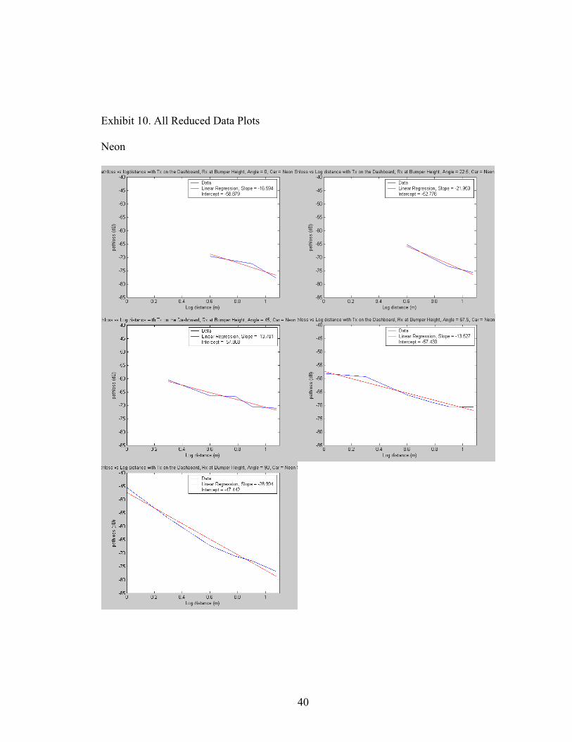
Exhibit 10. All Reduced Data Plots Neon

41

42

43

44

45

46

47

48

49

50
RAV4

51

52

53

54

55

56

57

58

59

60
Sundance

61

62

63

64

65

66

67

68

69