11 India KLEMS Labour Input- Quantity and Quality by Industry Suresh Aggarwal First World KLEMS...
31
1 1 India KLEMS Labour Input- Quantity and Quality by Industry Suresh Aggarwal First World KLEMS conference Harvard University 19-20 August 2010 Research assistance by Gunajit Kalita in creating the India KLEMS Labour Input dataset
-
Upload
sydney-sanders -
Category
Documents
-
view
222 -
download
2
Transcript of 11 India KLEMS Labour Input- Quantity and Quality by Industry Suresh Aggarwal First World KLEMS...

11
India KLEMS
Labour Input- Quantity and Quality by Industry
Suresh Aggarwal
First World KLEMS conferenceHarvard University
19-20 August 2010Research assistance by Gunajit Kalita in creating the
India KLEMS Labour Input dataset

22
Objectives-India KLEMS
To create a comprehensive data base on productivity growth using Growth Accounting Approach.
Construct a Time Series data on output, capital, labour, labour quality and intermediate inputs.

33
Major tasks for Data Base on Labour
Make a Time series of Employment from 1980 to 2004.
Prepare a Labour Quality Index from 1980 to 2004.
Make a Time series of Labour Input from 1980 to 2004.
Major Contributions of the PaperEfforts have been made for the first time to
estimate employment in Hours.Average number of Hours worked in a day
have been estimated for the first time.Both the Quinquennial and the annual
rounds have been used, for the first time for constructing the time series of employment.
A separate decomposition of Labour Quality into indices of age, sex and education has been attempted.
4
55
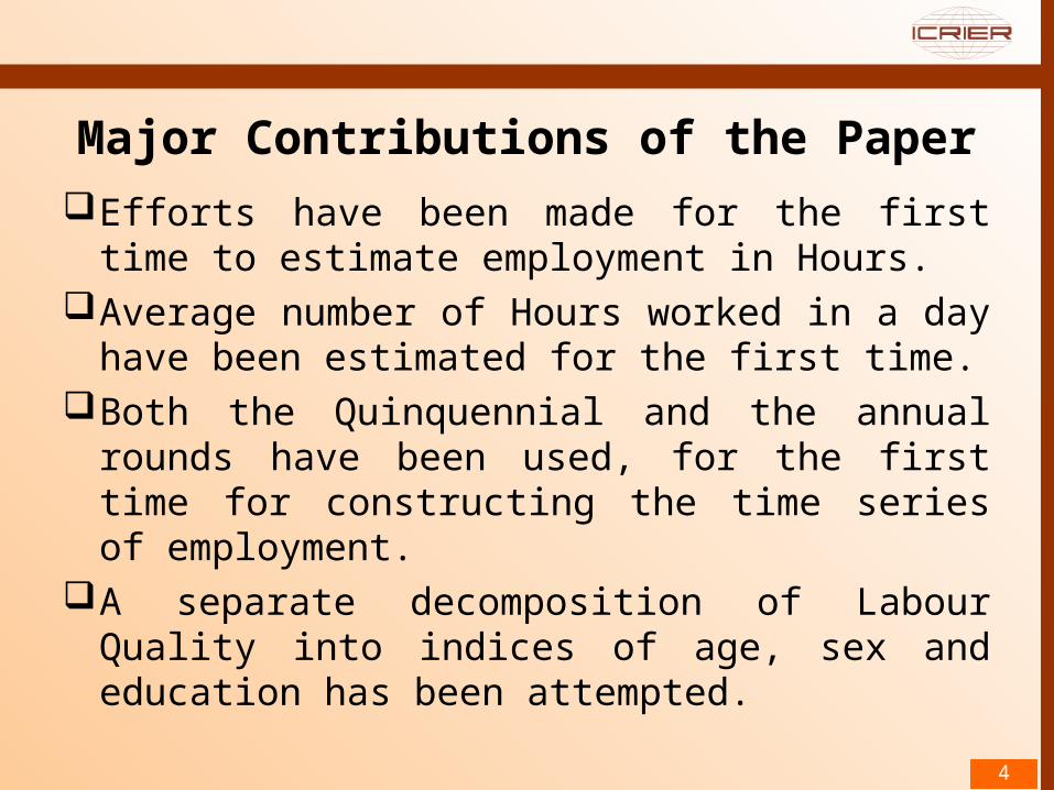
Gender: Males/Females Age : <29; 30-49; and 50+ Education: Up to Primary; From
Primary to Higher Secondary; and above Higher Secondary.
Sectors : 31 sectors.So it is 2*3*3*31 classification.
Broad classifications for all the series

66
Major Sources of Data Used For all sectors of the economy Employment
and Unemployment Surveys (EUS) by National Sample Survey Organization (NSSO) and Population Census. The two are Household/Individual specific.
Manufacturing Sector: Organized Manufacturing industries-
Annual Survey of Industries(ASI) by Central Statistical Organization (CSO).
Unorganized Manufacturing industries- Residual.

7
Methodology for Constructing the Time Series of Employment
Time Series of employment requires estimation of:a) Number of persons, and b) Total days and hours worked by each person.Time Series of Labour Input- Number of persons employedIn India, the number of employed may be estimated from Census and/or from EUS.While Census has been held every ten years, NSSO has conducted both major (or Quinquennial) and thin (or annual) rounds of EUS.
7
88
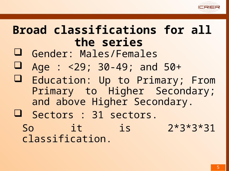
Employment Unemployment Survey (EUS)
Major (Quinquennial) Rounds of EUS since 1980: 38th (1983), 43rd(1987-88), 50th(1993-94),
55th (1999-00) and 61st(2004-05). Thin (Annual) Rounds: 45th to 60th .
EUS uses Usual Status [Usual Principal Status(UPS) and Usual Principal & Subsidiary Status (UPSS)], Current Weekly Status(CWS) and Current Daily Status (CDS) measures for Quinquennial (or major) rounds and Usual Status & CWS for annual (thin) rounds.
While UPS, UPSS and CWS measure number of persons, the CDS gives number of jobs.
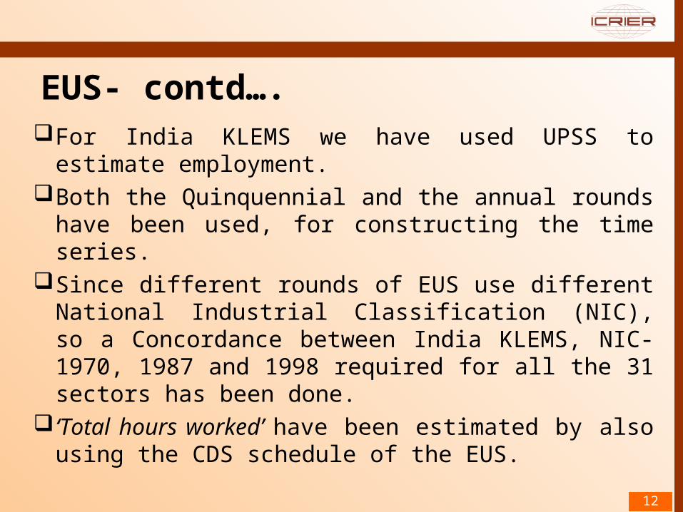
EUS- contd….For India KLEMS we have used UPSS to
estimate employment.Both the Quinquennial and the annual rounds
have been used, for constructing the time series.
Since different rounds of EUS use different National Industrial Classification (NIC), so a Concordance between India KLEMS, NIC-1970, 1987 and 1998 required for all the 31 sectors has been done.
‘Total hours worked’ have been estimated by also using the CDS schedule of the EUS.
12

17
Estimation of EmploymentEmployment has been computed as follows:I. Used; like all the previous studies, the Work
Participation Rates (WPRs) by UPSS from EUS and applied them to the corresponding period’s population of Rural Male, Rural Female, Urban Male and Urban Female to find out the number of workers in the four segments .
II.Use the 31-industry distribution of Employment from EUS and used these to the number of workers in step I and obtained Lij for each industry where i=1 for rural and 2 for urban sectors, and j=1 for male and 2 for female.
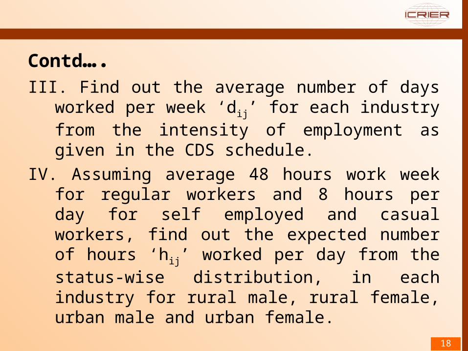
Contd….III. Find out the average number of days
worked per week ‘dij’ for each industry from the intensity of employment as given in the CDS schedule.
IV. Assuming average 48 hours work week for regular workers and 8 hours per day for self employed and casual workers, find out the expected number of hours ‘hij’ worked per day from the status-wise distribution, in each industry for rural male, rural female, urban male and urban female.
18

Contd….V. From the major rounds separate
interpolation of Lij ; dij; and hij was done for rural male, rural female, urban male and urban female to obtain the respective time series.
VI.Broad Industrial distribution from annual rounds was used as a control total on the corresponding interpolated Lij and revised numbers were obtained.
VII. Total person hours in a year were obtained for each industry as the sum of the products of revised Lij; dij; and hij over gender and sectors. ΣiΣjLij*dij*hij*52 19

Time Series of Labour Quality Index Quality Index has been constructed using the standard
methodology given by Jorgenson, et al (1987), which uses the Tornqvist translog index.
Analogously, other first order contributions by gender, age and education, Qs , Qa, and Qe , have also been computed.
Data required for Quality Index is:
Since the required labour composition data is available only from major rounds of EUS, so
Only Major rounds have been used for estimating the indices and the indices have been interpolated to get the time series for the entire period.
Only for aggregate 31 sectors- not for organized and unorganized separately.
20
a) Employment by sex by age by education by industry;b) Earnings for each of these cells.

24
Earnings Data
NSSO’s EUS relates earnings to only regular- salaried workers and casual workers.
The issue was how to estimate earnings of self employed.
The present study has used the Mincer Wage equation for the same and sample selection bias has been corrected for by using Heckman's two step procedure.
Earnings of Self Employed is required for quality index and labour compensation.

Results
Results are presented as follows:Firstly, for the Total economy.Secondly, by the broad industrial classification.Lastly, by the 31 KLEMS industrial classification.
27

Workforce Participation rate in different NSSO rounds (% of Total
Population)
29

Labour Input and Quality Change for the Total
Economy
30
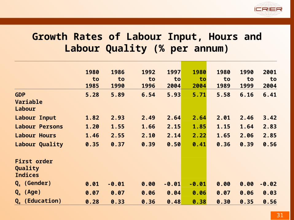
Growth Rates of Labour Input, Hours and Labour Quality (% per annum)
1980to
1985
1986to
1990
1992to
1996
1997to
2004
1980to
2004
1980to
1989
1990to
1999
2001to
2004GDP 5.28 5.89 6.54 5.93 5.71 5.58 6.16 6.41Variable Labour Labour Input 1.82 2.93 2.49 2.64 2.64 2.01 2.46 3.42Labour Persons 1.20 1.55 1.66 2.15 1.85 1.15 1.64 2.83Labour Hours 1.46 2.55 2.10 2.14 2.22 1.65 2.06 2.85Labour Quality 0.35 0.37 0.39 0.50 0.41 0.36 0.39 0.56 First order Quality IndicesQs (Gender) 0.01 -0.01 0.00 -0.01 -0.01 0.00 0.00 -0.02Qa (Age) 0.07 0.07 0.06 0.04 0.06 0.07 0.06 0.03Qe (Education) 0.28 0.33 0.36 0.48 0.38 0.30 0.35 0.56
31

Total Employment (persons and million hours) and hours per day
32
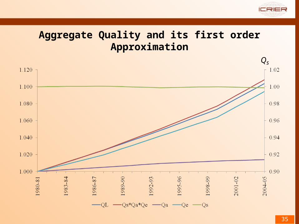
Aggregate Quality and its first order Approximation
35
sQ

Comparison with two other major studies
36
Author Period Growth rate in
Employment Index
Growth in Education
Index
Growth in Labour Input
Index
Bosworth; Collins & Virmani
(2007)
1980-2004 2.00 0.40 -
Sivasubramonian
(2004)
1980 to
1999
1.74 0.34 2.22
1980 to
1990
2.02 0.31 2.47
1990 to
1999
1.43 0.37 1.93
Current study (2010) 1980 to
2004
1.85 0.38 2.64
1980 to
1989
1.15 0.30 2.01
1990 to
1999*
1.64 0.35 2.46
The results for employment growth are different from Sivasubramonian’s study, but are close with Bosworth; Collins & Virmani (BCV).
The results for education growth rates are however, very close.
*Year 1991 has been excluded from the current study because of it being an abnormal year
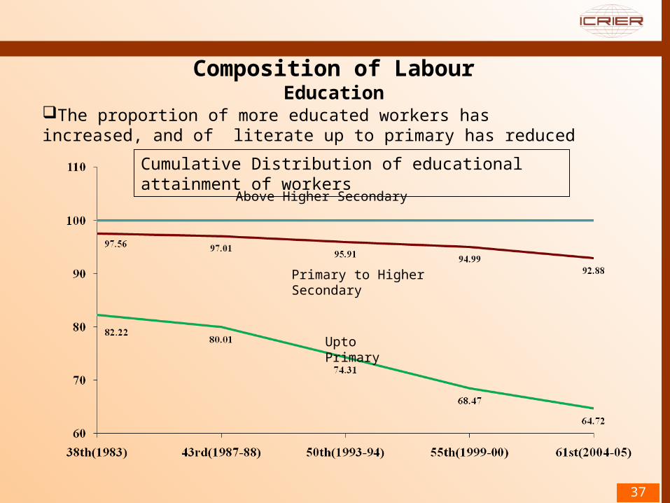
Composition of LabourEducation
37
The proportion of more educated workers has increased, and of literate up to primary has reduced
Above Higher Secondary
Primary to Higher Secondary
Upto Primary
Cumulative Distribution of educational attainment of workers

Gender: Female’s share of workforce, relative wages, days and hours
43
Days Per Week Ratio
Wage Ratio
Share of Workforce
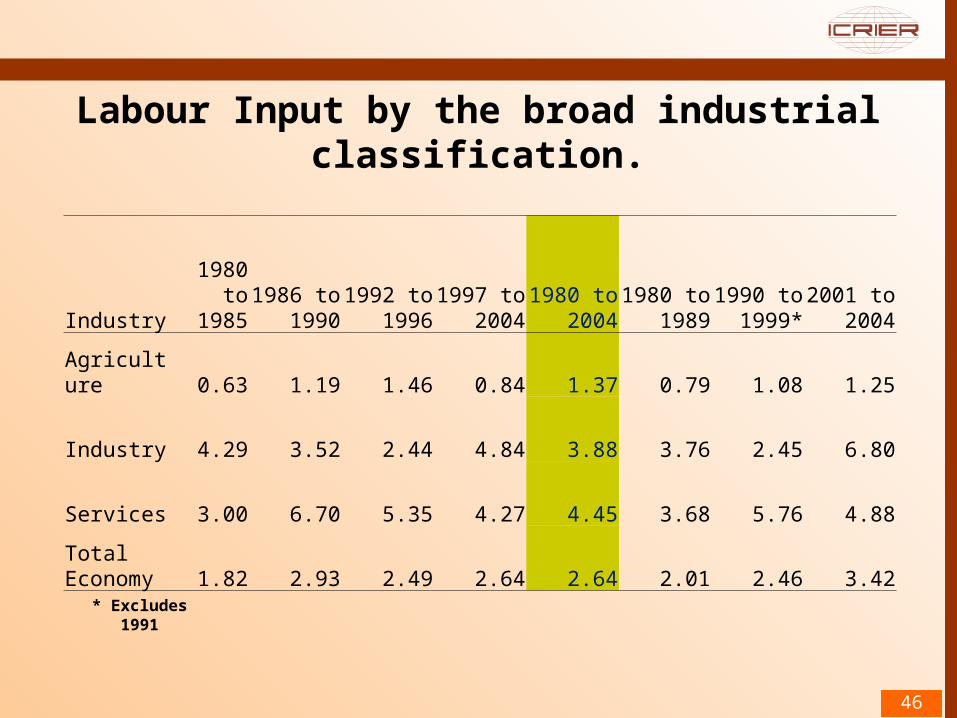
Labour Input by the broad industrial classification.
Industry
1980 to
19851986 to
19901992 to
19961997 to
20041980 to
20041980 to
19891990 to
1999*2001 to
2004
Agriculture 0.63 1.19 1.46 0.84 1.37 0.79 1.08 1.25
Industry 4.29 3.52 2.44 4.84 3.88 3.76 2.45 6.80
Services 3.00 6.70 5.35 4.27 4.45 3.68 5.76 4.88
Total Economy 1.82 2.93 2.49 2.64 2.64 2.01 2.46 3.42
46
* Excludes 1991
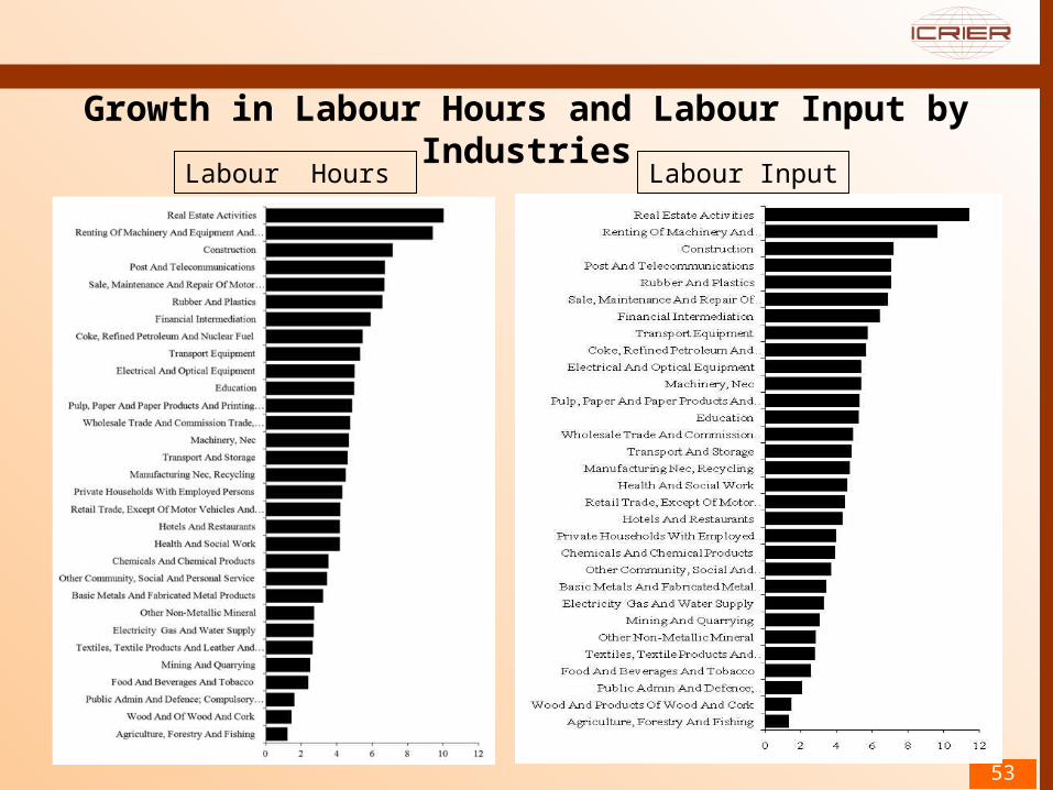
Growth in Labour Hours and Labour Input by Industries
53
Labour InputLabour Hours
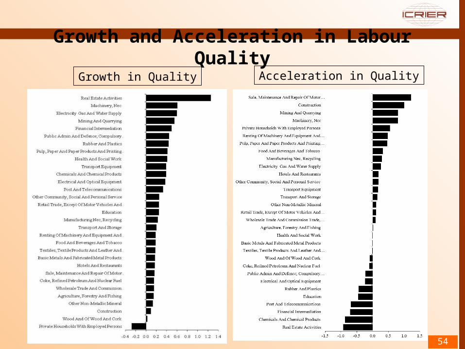
Growth and Acceleration in Labour Quality
54
Growth in Quality Acceleration in Quality

Labour Quality in Industries
The growth in labour quality was fastest in real estate activities; machinery; electricity, gas & water supply; and financial intermediation and very slow in wood & products of wood; construction; non-metallic minerals, agriculture and wholesale trade & commission.
The growth in labour quality was only 0.19 per cent in the pre reform period and it increased to 0.29 in the post reform decade indicating change in the composition of the workforce.
55

Contd….
The inter industry differences in the pattern of change in growth rate shows that the variation in growth rates has reduced over the period
The industries with either negative or very low growth rate in the first sub period (Sale, maintenance of motor vehicles etc., Construction, mining & quarrying, etc.) have generally been able to pick up the growth rate in the last period.
The reverse has also happened where the growth rate in labour quality for these industries has slowed down over the period (real estate, chemicals & chemical products, financial intermediation, etc.).
56

Manufacturing Employment- Organized & Unorganized Sector
60
Conclusion The WFPR remained almost unchanged over the period. The share of 30-49 age-group is highest. The share of educated workforce has gradually
increased during the period. There is a tendency for the share of female workers to
increase, though the share is still less than half to that of males.
Nominal Wages are generally higher for more educated and experienced workers.
Along with increase in employment of labour hours there has also been increase in labour quality, leading to a faster growth of labour input.
The share of unorganized employment has increased in the Indian manufacturing sector.
61

6262