10/11/01CSE 260 - Models CSE 260 – Introduction to Parallel Computation Topic 6: Models of...
41
10/11/01 CSE 260 - Models CSE 260 – Introduction to Parallel Computation Topic 6: Models of Parallel Computers October 11-18, 2001
-
date post
19-Dec-2015 -
Category
Documents
-
view
227 -
download
0
Transcript of 10/11/01CSE 260 - Models CSE 260 – Introduction to Parallel Computation Topic 6: Models of...
10/11/01 CSE 260 - Models
CSE 260 – Introduction to Parallel Computation
Topic 6: Models of Parallel Computers
October 11-18, 2001
CSE 260 - Models2
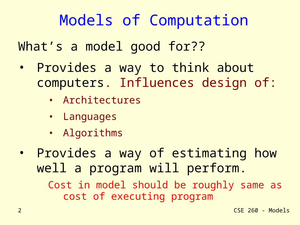
Models of Computation
What’s a model good for??
• Provides a way to think about computers. Influences design of:
• Architectures
• Languages
• Algorithms
• Provides a way of estimating how well a program will perform.
Cost in model should be roughly same as cost of executing program

CSE 260 - Models3
Outline
• RAM model of sequential computing
• PRAM
• Fat tree
• PMH
• BSP
• LogP

CSE 260 - Models4
The Random Access Machine Model
RAM model of serial computers:– Memory is a sequence of words, each
capable of containing an integer.
– Each memory access takes one unit of time
– Basic operations (add, multiply, compare) take one unit time.
– Instructions are not modifiable
– Read-only input tape, write-only output tape

CSE 260 - Models5
Has RAM influenced our thinking?
Language design:
No way to designate registers, cache, DRAM.
Most convenient disk access is as streams.
How do you express atomic read/modify/write?
Machine & system design:
It’s not very easy to modify code.
Systems pretend instructions are executed in-order.
Performance Analysis:
Primary measures are operations/sec (MFlop/sec, MHz, ...)
What’s the difference between Quicksort and Heapsort??

CSE 260 - Models6
What about parallel computers
• RAM model is generally considered a very successful “bridging model” between programmer and hardware.
• “Since RAM is so successful, let’s generalize it for parallel computers ...”
CSE 260 - Models7
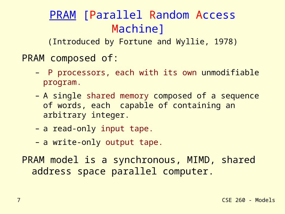
PRAM [Parallel Random Access Machine]
PRAM composed of:– P processors, each with its own unmodifiable
program.
– A single shared memory composed of a sequence of words, each capable of containing an arbitrary integer.
– a read-only input tape.
– a write-only output tape.
PRAM model is a synchronous, MIMD, shared address space parallel computer.
(Introduced by Fortune and Wyllie, 1978)
CSE 260 - Models8
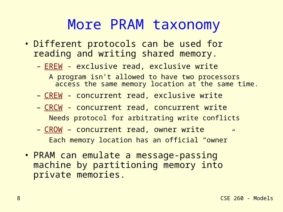
More PRAM taxonomy• Different protocols can be used for reading
and writing shared memory.– EREW - exclusive read, exclusive write
A program isn’t allowed to have two processors access the same memory location at the same time.
– CREW - concurrent read, exclusive write
– CRCW - concurrent read, concurrent write Needs protocol for arbitrating write conflicts
– CROW – concurrent read, owner writeEach memory location has an official “owner”
• PRAM can emulate a message-passing machine by partitioning memory into private memories.
CSE 260 - Models9
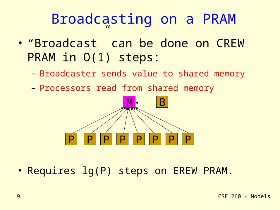
Broadcasting on a PRAM
• “Broadcast” can be done on CREW PRAM in O(1) steps:– Broadcaster sends value to shared memory
– Processors read from shared memory
• Requires lg(P) steps on EREW PRAM.
M
PPPPPPPP
B
CSE 260 - Models10
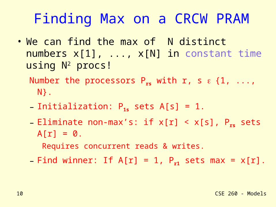
Finding Max on a CRCW PRAM
• We can find the max of N distinct numbers x[1], ..., x[N] in constant time using N2 procs!
Number the processors Prs with r, s {1, ..., N}.
– Initialization: P1s sets A[s] = 1.
– Eliminate non-max’s: if x[r] < x[s], Prs sets A[r] = 0.Requires concurrent reads & writes.
– Find winner: If A[r] = 1, Pr1 sets max = x[r].
CSE 260 - Models11
Some questions
1. What if the x[i]’s aren’t necessarily distinct?
2. Can you sort N numbers in constant time?
And only use only Nk processors (for some k)?
3. How fast can you sort on CREW?
4. Does any of this have any practical significance ????
CSE 260 - Models12
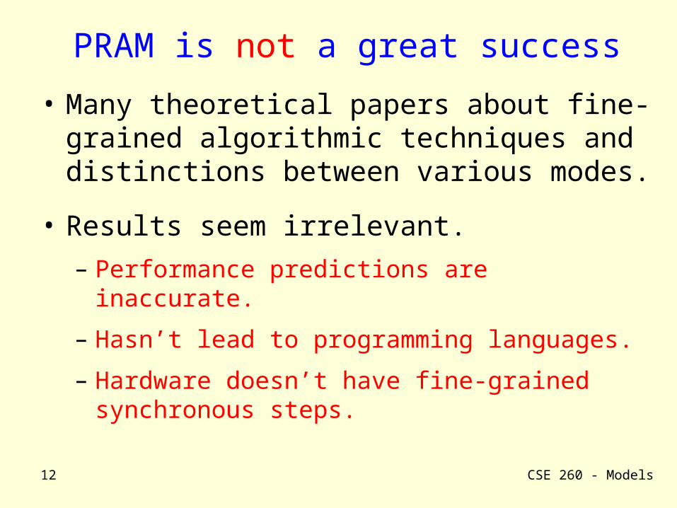
PRAM is not a great success
• Many theoretical papers about fine-grained algorithmic techniques and distinctions between various modes.
• Results seem irrelevant. – Performance predictions are inaccurate.
– Hasn’t lead to programming languages.
– Hardware doesn’t have fine-grained synchronous steps.
CSE 260 - Models13
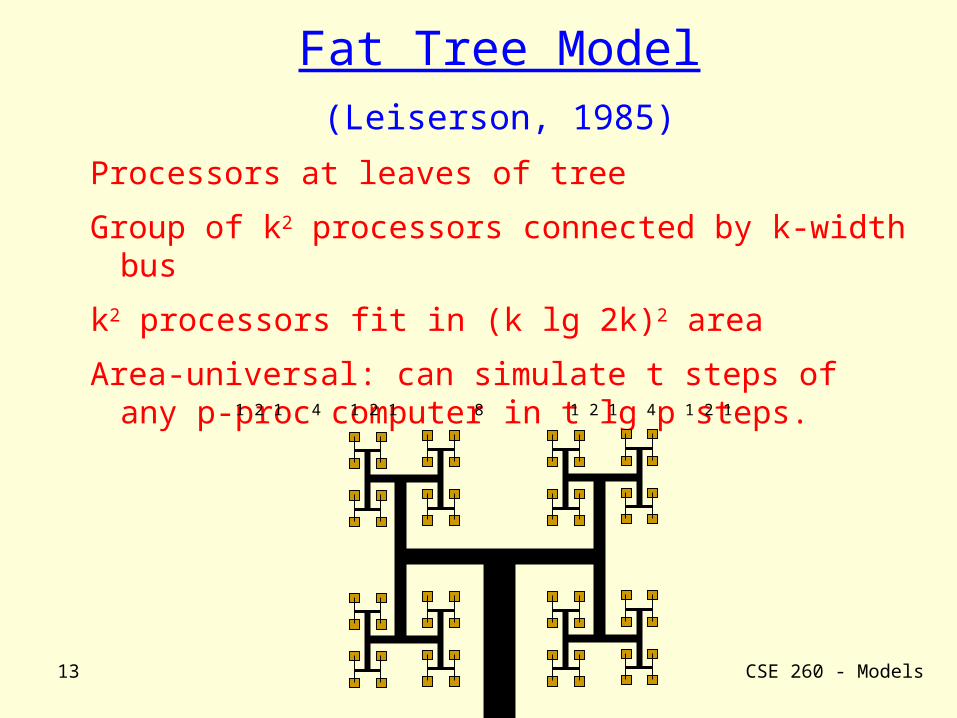
Fat Tree Model(Leiserson, 1985)
Processors at leaves of tree
Group of k2 processors connected by k-width bus
k2 processors fit in (k lg 2k)2 area
Area-universal: can simulate t steps of any p-proc computer in t lg p steps.
1 2 1 4 1 2 1 8 1 2 1 4 1 2 1
CSE 260 - Models14
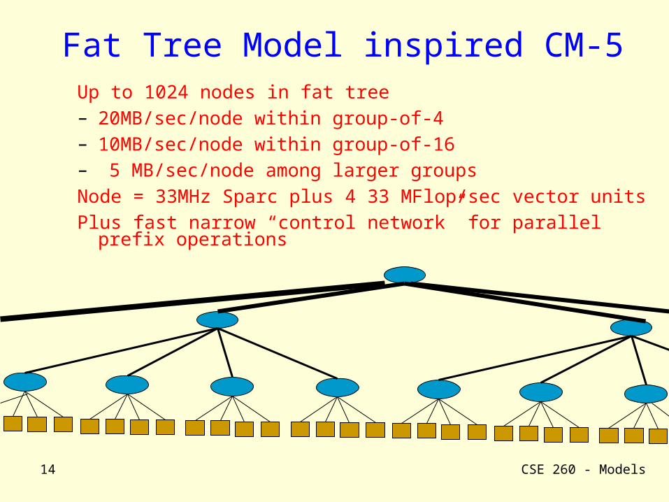
Fat Tree Model inspired CM-5Up to 1024 nodes in fat tree – 20MB/sec/node within group-of-4– 10MB/sec/node within group-of-16– 5 MB/sec/node among larger groupsNode = 33MHz Sparc plus 4 33 MFlop/sec vector units Plus fast narrow “control network” for parallel prefix
operations
CSE 260 - Models15
What happened to fat trees?
• CM-5 had many interesting features– Active message VSM software layer.– Randomized routing.– Fast control network.
• It was somewhat successful, but died anyway– Using the floating point unit well wasn’t easy.– Perhaps not sufficiently COTS-like to compete.
• Fat trees live on, but aren’t highlighted ...– IBM SP and others have less bandwidth between
cabinets than within a cabinet.
– Seen more as a flaw than a feature.

CSE 260 - Models16
Another look at the RAM model
• RAM analysis says matrix multiply is O(N3).for i = 1 to N for j = 1 to N for k = 1 to N C[i,j] += A[i,k]*B[k,j]
• Is it??

CSE 260 - Models17
Matrix Multiply on RS/6000
- 2
0
2
4
6
0 2 4 6
log Problem Size
log
cycl
es/fl
opT = N4.7
O(N3) performance would have constant cycles/flopPerformance looks much closer to O(N5)
Size 2000 took 5 days
12000 would take1095 years

CSE 260 - Models18
Column major storage layout
cachelines
Blue row of matrix is stored in red cacheline

CSE 260 - Models19
Memory Accesses in Matrix Multiplyfor i = 1 to N for j = 1 to N for k = 1 to N C[i,j] += A[i,k]*B[k,j]
When cache (or TLB or memory) can’t hold entire B matrix, there will be a miss on every line.
When cache (or TLB or memory) can’t hold a row of A, there will be a miss on each access
Sequentialaccess throughentire matrix
Stride-Naccess toone row*
* assumes data is in column-major order
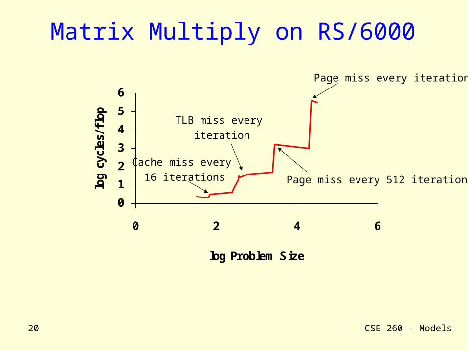
CSE 260 - Models20
Matrix Multiply on RS/6000
0
1
2
3
4
5
6
0 2 4 6
log Problem Size
log
cycl
es/fl
op
Page miss every 512 iterations
Page miss every iteration
TLB miss every iteration
Cache miss every 16 iterations
CSE 260 - Models21
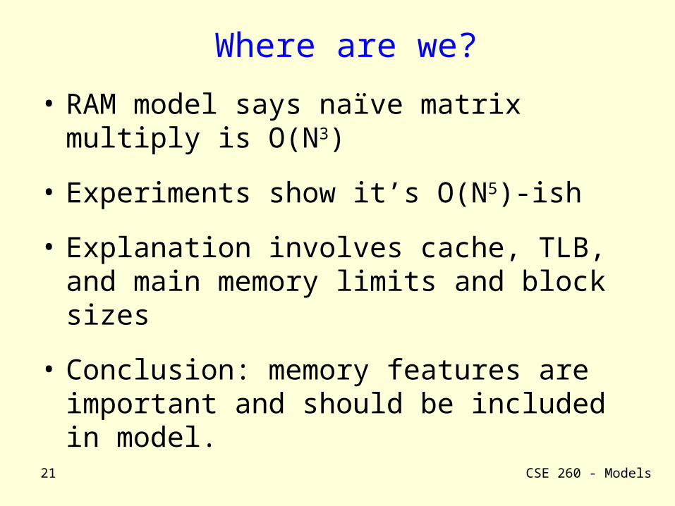
Where are we?
• RAM model says naïve matrix multiply is O(N3)
• Experiments show it’s O(N5)-ish
• Explanation involves cache, TLB, and main memory limits and block sizes
• Conclusion: memory features are important and should be included in model.
CSE 260 - Models22
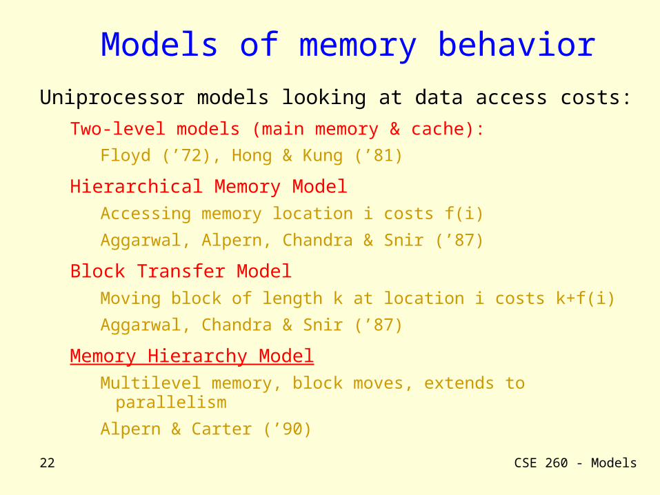
Models of memory behavior
Uniprocessor models looking at data access costs:
Two-level models (main memory & cache):
Floyd (’72), Hong & Kung (’81)
Hierarchical Memory ModelAccessing memory location i costs f(i)
Aggarwal, Alpern, Chandra & Snir (’87)
Block Transfer ModelMoving block of length k at location i costs k+f(i)
Aggarwal, Chandra & Snir (’87)
Memory Hierarchy ModelMultilevel memory, block moves, extends to parallelism
Alpern & Carter (’90)

CSE 260 - Models23
Memory Hierarchy model
A uniprocessor is
Sequence of memory modulesHighest level is large memory, low
speedProcessor (level 0) is tiny memory,
high speed
Connected by channels All channels can be active
simultaneously
Data are moved in fixed-sized blocks
A block is a chunk of contiguous dataBlock size depends on level
DISK
DRAM
cache
regs
CSE 260 - Models24
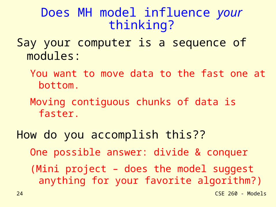
Does MH model influence your thinking?
Say your computer is a sequence of modules:
You want to move data to the fast one at bottom.
Moving contiguous chunks of data is faster.
How do you accomplish this??
One possible answer: divide & conquer
(Mini project – does the model suggest anything for your favorite algorithm?)

CSE 260 - Models25
Visualizing Matrix Multiplication
C
B
A
“stick” of computationis dot product of a
row of A with column of B
cij= aikbkj
i
j C = A B

CSE 260 - Models26
Visualizing Matrix Multiplication
C
B
A
“Cubelet” of computationis product of a submatrixof A with submatrix of B - Data involved is proportional to surface area. - Computation is proportional to volume.
CSE 260 - Models27
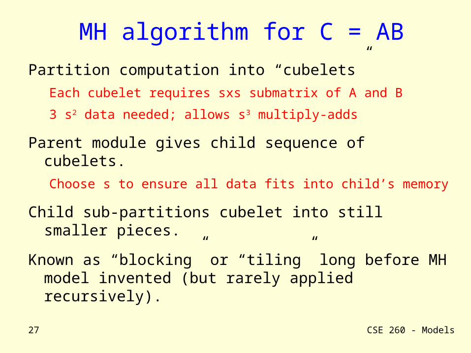
MH algorithm for C = AB
Partition computation into “cubelets”
Each cubelet requires sxs submatrix of A and B
3 s2 data needed; allows s3 multiply-adds
Parent module gives child sequence of cubelets.
Choose s to ensure all data fits into child’s memory
Child sub-partitions cubelet into still smaller pieces.
Known as “blocking” or “tiling” long before MH model invented (but rarely applied recursively).
CSE 260 - Models28
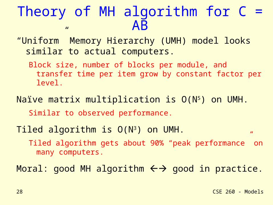
Theory of MH algorithm for C = AB
“Uniform” Memory Hierarchy (UMH) model looks similar to actual computers.
Block size, number of blocks per module, and transfer time per item grow by constant factor per level.
Naïve matrix multiplication is O(N5) on UMH.
Similar to observed performance.
Tiled algorithm is O(N3) on UMH.
Tiled algorithm gets about 90% “peak performance” on many computers.
Moral: good MH algorithm good in practice.

CSE 260 - Models29
Visualizing computers in MH model Height of module = lg(blocksize)
Width = lg(number of blocks)
Length of channel = lg(transfer time)
DISK
DRAM
cache
regs
This computer is reasonably well-balanced
This one isn’t
Doesn’t satisfy “widecache principle” (squaresubmatrices don’t fit).
Bandwidth too low
CSE 260 - Models30
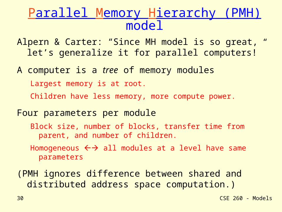
Parallel Memory Hierarchy (PMH) model
Alpern & Carter: “Since MH model is so great, let’s generalize it for parallel computers!”
A computer is a tree of memory modulesLargest memory is at root.
Children have less memory, more compute power.
Four parameters per moduleBlock size, number of blocks, transfer time from parent, and
number of children.
Homogeneous all modules at a level have same parameters
(PMH ignores difference between shared and distributed address space computation.)

CSE 260 - Models31
Some Parallel Architectures
The Grid
registers
Mainmemories
DisksCaches
network
NOW
DISKS
Mainmemories
Shareddisk
system
DisksDisksCaches
network
Mainmemory
DISK
Scalar cache
Extended Storage
vector regs
Vector supercomputer
CSE 260 - Models32
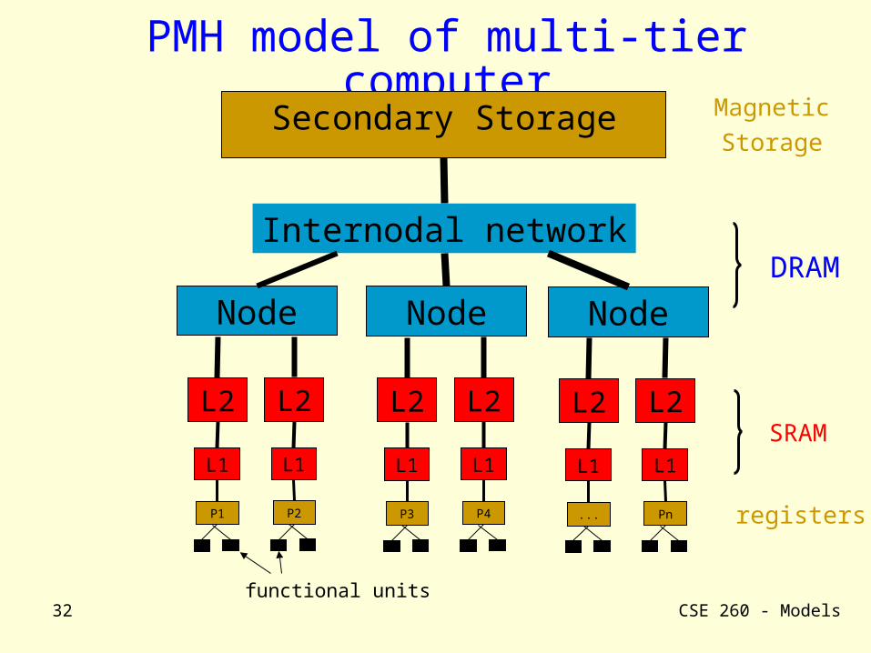
PMH model of multi-tier computerSecondary Storage
Internodal network
Node
L2
L1
P1
L2
L1
P2
Node
L2
L1
P3
L2
L1
P4
Node
L2
L1
...
L2
L1
Pn
functional units
DRAM
SRAM
MagneticStorage
registers
CSE 260 - Models33
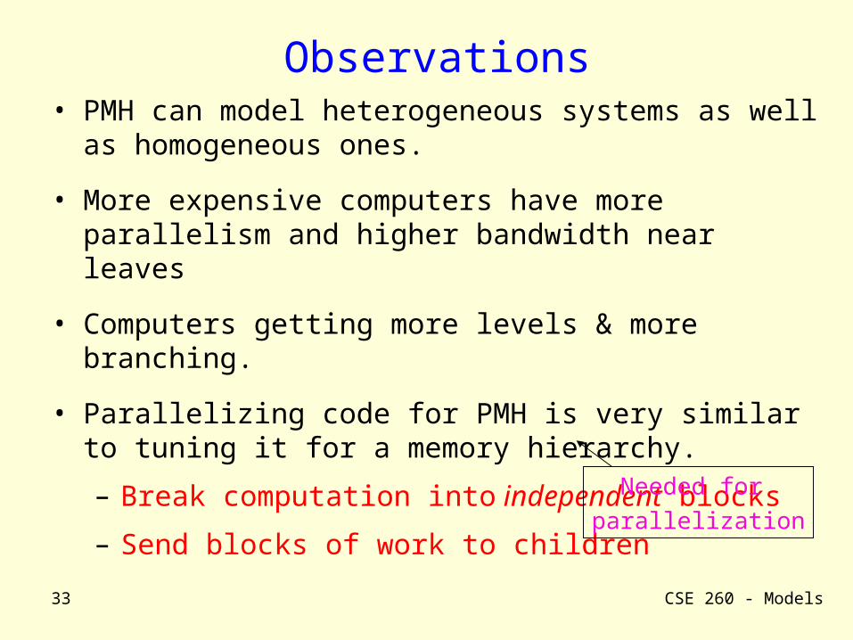
Observations• PMH can model heterogeneous systems as well as
homogeneous ones.
• More expensive computers have more parallelism and higher bandwidth near leaves
• Computers getting more levels & more branching.
• Parallelizing code for PMH is very similar to tuning it for a memory hierarchy.
– Break computation into independent blocks
– Send blocks of work to children Needed for parallelization
CSE 260 - Models34
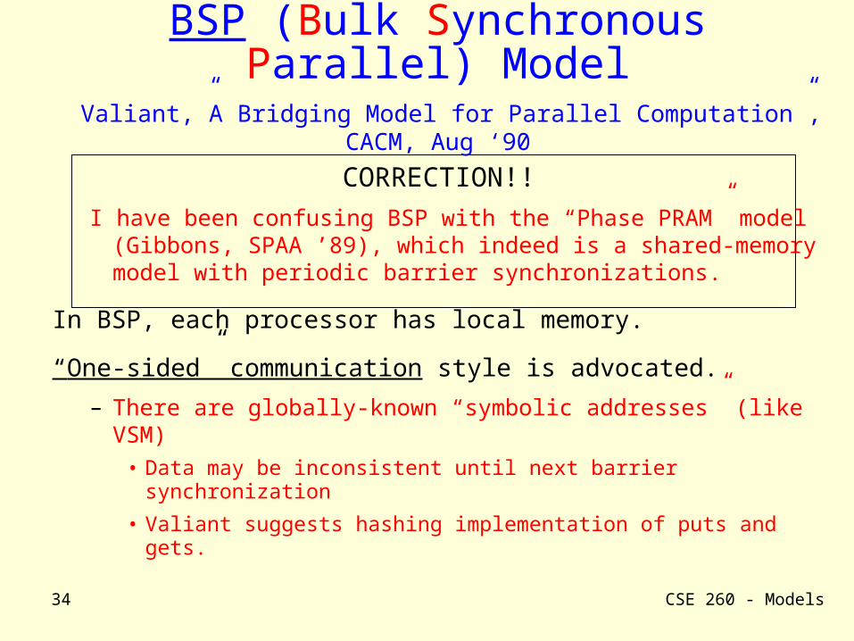
BSP (Bulk Synchronous Parallel) Model
Valiant,”A Bridging Model for Parallel Computation”, CACM, Aug ‘90
CORRECTION!!
I have been confusing BSP with the “Phase PRAM” model (Gibbons, SPAA ’89), which indeed is a shared-memory model with periodic barrier synchronizations.
In BSP, each processor has local memory.
“One-sided” communication style is advocated.
– There are globally-known “symbolic addresses” (like VSM)• Data may be inconsistent until next barrier synchronization
• Valiant suggests hashing implementation of puts and gets.

CSE 260 - Models35
BSP Programs
• BSP programs composed of supersteps.
• In each superstep, processors execute up to L computational steps using locally stored data, and also can send and receive messages
• Processors synchronize at end of superstep (at which time all messages have been received)
• Oxford BSP is a library of C routines for implementing BSP programs. It provides:
– Direct Remote Memory Access (a VSM layer)
– Bulk Synchronous Message Passing (sort of like non-blocking message passing in MPI)
superstep
synch
superstep
synch
superstep
synch

CSE 260 - Models36
Parameters of BSP ModelP = number of processors.
s = processor speed (steps/second).
observed, not “peak”.
L = time to do a barrier synchronization (steps/synch).
g = cost of sending message (steps/word).
measure g when all processors are communicating.
h0 = minimum # of messages per superstep.
For h h0, cost of sending h messages is hg.
h0 is similar to block size in PMH model.

CSE 260 - Models37
BSP Notes
• Number of processors in model can be greater than number of processors of machine.
Easier for computer to complete the remote memory operations
• Not all processors need to join barrier synch
• Time for superstep = 1/s (max (operations performed by any processor)
+ g max (messages sent or received by a
processor, h0)
+ L)
CSE 260 - Models38
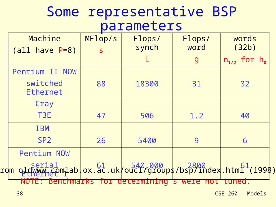
Some representative BSP parameters
Machine
(all have P=8)
MFlop/s
s
Flops/synch
L
Flops/word
g
words (32b)
n1/2 for h0
Pentium II NOW
switched Ethernet
88 18300 31 32
Cray
T3E 47 506 1.2 40
IBM
SP2 26 5400 9 6
Pentium NOW
serial Ethernet 1 61 540,000 2800 61From oldwww.comlab.ox.ac.uk/oucl/groups/bsp/index.html (1998)
NOTE: Benchmarks for determining s were not tuned.
CSE 260 - Models39
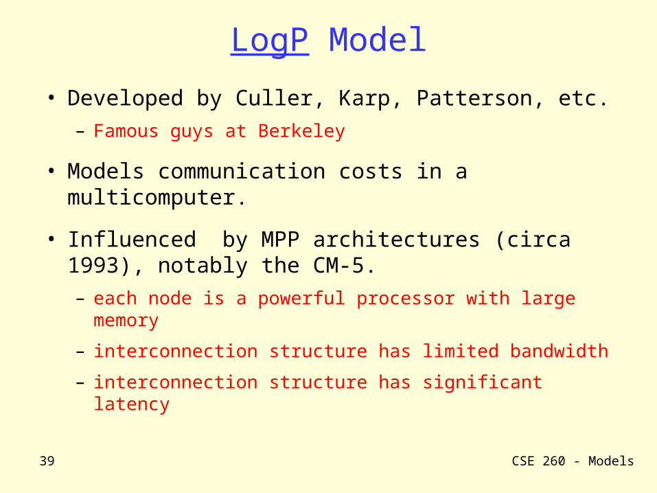
LogP Model
• Developed by Culler, Karp, Patterson, etc.– Famous guys at Berkeley
• Models communication costs in a multicomputer.
• Influenced by MPP architectures (circa 1993), notably the CM-5.– each node is a powerful processor with large
memory
– interconnection structure has limited bandwidth
– interconnection structure has significant latency

CSE 260 - Models40
LogP parameters• L: latency – time for message to go from
Psender to Preceiver
• o: overhead - time either processor is occupied sending or receiving message– Processor can’t do anything else for o cycles.
• g: gap - minimum time between messages– Processor can have at most L/g messages in
transit at a time.
– Gap includes overhead time (so overhead gap)
• P: number of processors
L, o, and g are measured in cycles

CSE 260 - Models41
Efficient Broadcasting in LogP
P0P1P2P3P4P5P6P7
time
og
og
og
oo
o
o o
L
LL
oLL
o og
oo
L
o
L
Picture shows P=8, L=6, g=4, o=2
208 164 12 24


![Index [complements.lavoisier.net] · Subcanopy and Subsurface (AirMOSS) 260–261 airborne sensors AirMOSS 260–261 E‐SAR/F‐SAR/PLMR2, 261–262 and features 260 HyMap 259–260](https://static.fdocuments.in/doc/165x107/5e3275efbac565760d5b4a2e/index-subcanopy-and-subsurface-airmoss-260a261-airborne-sensors-airmoss.jpg)