10.1 Van Horne and Wachowicz, Fundamentals of Financial Management, 13th edition. © Pearson...

10.1 Van Horne and Wachowicz, Fundamentals of Financial Management, 13th edition. © Pearson Education Limited 2009. Created by Gregory Kuhlemeyer.

Chapter 10Chapter 10

Accounts Receivable Accounts Receivable and Inventory and Inventory ManagementManagement

Accounts Receivable Accounts Receivable and Inventory and Inventory ManagementManagement


1. List the key factors that can be varied in a firm's credit policy and understand the trade-off between profitability and costs involved.

2. Understand how the level of investment in accounts receivable is affected by the firm's credit policies.

3. Critically evaluate proposed changes in credit policy, including changes in credit standards, credit period, and cash discount.

4. Describe possible sources of information on credit applicants and how you might use the information to analyze a credit applicant.

5. Identify the various types of inventories and discuss the advantages and disadvantages of increasing/decreasing inventories

6. Describe, explain, and illustrate the key concepts and calculations necessary for effective inventory management and control, including classification, economic order quantity (EOQ), order point, safety stock, and just-in-time (JIT).

After Studying Chapter 10, After Studying Chapter 10, you should be able to:you should be able to:


• Credit and Collection Policies

• Analyzing the Credit Applicant

• Inventory Management and Control

Accounts Receivable and Accounts Receivable and Inventory ManagementInventory Management


(1) Average Collection Period

(2) Bad-debtLosses

Quality ofQuality ofTrade AccountTrade Account

Length ofCredit Period

Possible CashDiscount

FirmCollectionProgram

Credit and Collection Credit and Collection Policies of the FirmPolicies of the Firm


The financial manager should continually lower the firm’s credit standards as long as profitability from the change exceeds the extra costs generated by the additional

receivables.

Credit StandardsCredit Standards – The minimum quality of credit worthiness of a credit applicant

that is acceptable to the firm.

Why lower the firm’s credit standards?Why lower the firm’s credit standards?

Credit StandardsCredit Standards


• A larger credit department

• Additional clerical work

• Servicing additional accounts

• Bad-debt losses

• Opportunity costs

Costs arising from relaxing Costs arising from relaxing credit standardscredit standards

Credit StandardsCredit Standards


Basket Wonders is not operating at full capacity Basket Wonders is not operating at full capacity and wants to determine if a relaxation of their and wants to determine if a relaxation of their credit standards will enhance profitability. credit standards will enhance profitability.

• The firm is currently producing a single product with variable costs of $20 and selling price of $25.

• Relaxing credit standards is not expected to affect current customer payment habits.

Example of Relaxing Example of Relaxing Credit StandardsCredit Standards


• Additional annual credit sales of $120,000 and an average collection period for new accounts of 3 months is expected.

• The before-tax opportunity cost for each dollar of funds “tied-up” in additional receivables is 20%.

Ignoring any additional bad-debt losses Ignoring any additional bad-debt losses that may arise, should Basket Wonders that may arise, should Basket Wonders

relax their credit standards?relax their credit standards?



Profitability of ($5 contribution) x (4,800 units) =additional sales $24,000$24,000(120,000/25 = 4,800 units)

Additional ($120,000 sales) / (4 Turns) =receivables $30,000(120,000/(3/12) = 30,000)

Investment in ($20/$25) x ($30,000) =add. receivables $24,000

Req. pre-tax return (20% opp. cost) x $24,000 =on add. investment $4,800$4,800(20% of additional investment)

Yes!Yes! Profits > Required pre-tax return




(2) Bad-debtLosses

Quality ofTrade Account

Length ofLength ofCredit PeriodCredit Period





Average Collection Period

The average length of time from a sale on credit until the payment becomes usable funds for the firm.

Two parts: Time from the sale until the customer mails

the payment Time from when the payment is mailed

until the firm has received the cleared funds in its bank account.


Average Collection Period

Objective is to collect accounts receivable as quickly as possible without losing sales from high pressure collection procedures. This involves three key areas: Credit Selection Credit Terms Credit Monitoring


Credit PeriodCredit Period – The total length of time over which credit is extended to a customer to

pay a bill. For example, “net 30” “net 30” requires full payment to the firm within 30 days from the

invoice date.

Credit Terms Credit Terms – Specify the length of time over which credit is extended to a customer

and the discount, if any, given for early payment. For example, “2/10, net 30.”“2/10, net 30.”

Credit TermsCredit Terms


Basket Wonders Basket Wonders is considering changing its credit period from “net 30” “net 30” (which has resulted in 12 A/R “Turns” per year) to “net 60” “net 60” (which is expected to result in 6 A/R “Turns” per year).

• The firm is currently producing a single product with variable costs of $20 and a selling price of $25.

• Additional annual credit sales of $250,000 from new customers are forecasted, in addition to the current $2 million in annual credit sales.

Example of Relaxing Example of Relaxing the Credit Periodthe Credit Period



Ignoring any additional bad-debt losses Ignoring any additional bad-debt losses that may arise, should Basket Wonders that may arise, should Basket Wonders

relax their credit period?relax their credit period?



Profitability of ($5 contribution)x(10,000 units) =additional sales $50,000$50,000(250,000/25 = 10,000)

Additional ($250,000 sales) / (6 Turns) =receivables $41,667

Investment in add. ($20/$25) x ($41,667) =receivables (new sales) $33,334

Previous ($2,000,000 sales) / (12 Turns) =receivable level $166,667



New ($2,000,000 sales) / (6 Turns) =receivable level $333,333

Investment in $333,333 - $166,667 =add. receivables $166,666 (original sales)

Total investment in $33,334 + $166,666 =add. receivables $200,000

Req. pre-tax return (20% opp. cost) x $200,000 =on add. investment $40,000$40,000

Yes! Yes! Profits > Required pre-tax return



Changing credit standards

Li Hong Company is currently selling a product for $10 per unit. Sales (all on credit) for last year were 60,000 units. The variable cost per unit is $6. The firm’s total fixed costs are $120,000.

The firm is considering a relaxation of credit standards that is expected to result in the following: a 5% increase in unit sales to 63,000 units; an increase in the average collection period from 30 days (its current level) to 45 days; an increase in bad-debt expenses from 1% of sales (the current level) to 2%. The firm’s required return on equal-risk investments, which is the opportunity cost of tying up funds in accounts receivable, is 15%.


Changing credit standards Need to calculate the effect on the firm’s additional profit

contribution from sales, the cost of the marginal investment in accounts receivable and the cost of marginal bad debts.

Additional profit contribution from sales Fixed costs are ‘sunk’ and thereby unaffected by a change in

the sales level. Variable cost is the only cost relevant to a change in sales.

Sales are expected to increase by 5%, or 3,000 units. The profit contribution per unit equals the difference between the sale price per unit ($10) and the variable cost per unit ($6) and so the profit contribution per unit will be $4.

Thus, the total additional profit contribution from sales will be $12,000 (3,000 units × $4 per unit).


Changing credit standards Cost of the marginal investment in accounts receivable To determine the cost of the marginal investment in accounts

receivable, Peng Xi must find the difference between the cost of carrying receivables before and after the introduction of the relaxed credit standards. We are only concerned about the out-of-pocket costs so the relevant cost in this analysis is the variable cost.

The average investment in accounts receivable can be calculated using the following formula:

Average investment in accounts receivable = total variable cost of annual sales/ turnover of accounts receivable

where Turnover of accounts receivable = 365/average collection

period


Changing credit standards The total variable cost of annual sales, using the variable cost

per unit of $6 are, Total variable cost of annual sales: Under present plan: ($6 × 60,000 units) = $360,000 Under proposed plan: ($6 × 63,000 units) = $378,000 The proposed plan increases total variable cost of sales by

$18,000. The turnover of accounts receivable shows the number of times

each year that accounts receivable are turned into cash. It is found by dividing the average collection period into 365.

Turnover of accounts receivable (rounded): Under present plan: 365/30 = 12.2 Under proposed plan: 365/45 = 8.1


Changing credit standards Substitute the cost and turnover data just calculated to get the

following average investments in accounts receivable: Average investment in accounts receivable: Under present plan: $360,000/12.2 = $29,508 Under proposed plan: $378,000/8.1 = $46,667 The marginal investment in accounts receivable, and its cost,

are calculated as follows: Cost of marginal investment in accounts receivable (A/R): Average investment under proposed plan $46,667 – Average investment under present plan 29,508 Marginal investment in accounts receivable $17,159 × Required return on investment 0.15 Cost of marginal investment in A/R $2,574


Changing credit standards The value of $2,574 is a cost because it represents the

maximum amount that could have been earned on the $17,159 had it been placed in the best equal-risk investment alternative available at the firm’s required return on investment of 15%.

Cost of marginal bad debts The cost of marginal bad debts is the difference between

the level of bad debts before and after the relaxation of credit standards:

Cost of marginal bad debts: Under proposed plan: 0.02 × $10 × 63,000 units = 12,600 Under present plan: 0.01 × $10 × 60,000 units = 6,000 Cost of marginal bad debts $6,600


Changing credit standards Bad debts costs are calculated by using the sale price per

unit ($10) to identify not just the true loss of variable (or out-of-pocket) cost ($6) that results when a customer fails to pay its account, but also the profit contribution per unit—in this case, $4 ($10 sales prices – $6 variable cost)—that is included in the ‘additional profit contribution from sales’. Thus, the resulting cost of marginal bad debts is $6,600.

To decide whether the firm should relax its credit standards, the additional profit contribution from sales must be compared with the sum of the cost of the marginal investment in accounts receivable and the cost of marginal bad debts. If the additional profit contribution is greater than marginal costs, credit standards should be relaxed.


Changing credit standards The effect of Li Hong’s credit relaxation policy:



(2) Bad-debtLosses



Possible CashPossible CashDiscountDiscount




Cash DiscountCash Discount – A percent (%) reduction in sales or purchase price allowed for early payment of invoices. For example, “2/10” “2/10”

allows the customer to take a 2% cash discount during the cash discount period.

Cash Discount PeriodCash Discount Period – The period of time during which a cash discount can be taken for

early payment. For example, “2/10”“2/10” allows a cash discount in the first 10 days from the

invoice date.



Credit TermsCredit Terms The terms of sale for customers who have been

extended credit by the firm. E.g. ‘net 30’ means the customer has 30 days from

the beginning of the credit period to pay the full invoice amount.

Some firms offer cash discounts as percentage discounts from the purchase price for full payment without a specified time.

E.g. ‘2/10 net 30’ means the customer can take a 2% discount from the amount payable if payment is made within the first 10 days of the credit period, or pay the full amount of the amount payable within 30 days of the beginning of the credit period.



Any discounts for early payment should only be offered after a cost benefit analysis.

Are reflective of the type of business the firm operates. E.g. seasonal, perishable goods etc

Should be reflective of industry standards at a firm level, but reflective of customer riskiness at an individual customer level.


Credit TermsCredit Terms Li Hong Company has an average collection period of 40 days

(turnover = 365/40 = 9.1). The firm’s credit terms are net 30, so this period is divided into 32 days until the customers place their payments in the mail (not everyone pays within 30 days) and 8 days to receive, process and collect payments once they are mailed. Li Hong is considering changing its credit terms from net 30 to 2/10 net 30. This change is expected to reduce the amount of time until the payments are placed in the mail, resulting in an average collection period of 25 days (turnover = 365/25 = 14.6).

As shown in the EOQ example (slide 74), Li Hong has a raw material with current annual usage of 1,100 units. Each finished product produced requires one unit of this raw material at a variable cost of $1,500 per unit, incurs another $800 of variable cost in the production process and sells for $3,000 on terms of net 30. Li Hong estimates that 80% of its customers will take the 2% discount and that offering the discount will increase sales of the finished product by 50 units (from 1,100 to 1,150 units) per year but will not alter its bad-debt percentage. Li Hong’s opportunity cost of funds invested in accounts receivable is 14%. Should Li Hong offer the proposed cash discount?


Credit TermsCredit Terms Analysis of initiating a cash discount for Li Hong Company

c Li Hong’s opportunity cost of funds is 14%


A competing firm of Basket Wonders is considering changing the credit period from “net “net

60” 60” (which has resulted in 6 A/R “Turns” per year) to “2/10, net 60.”“2/10, net 60.”

• Current annual credit sales of $5 million are expected to be maintained.

• The firm expects 30% of its credit customers (in dollar volume) to take the cash discount and thus increase A/R “Turns” to 8.

• (30% x 10 days + 70% x 60 days = 3 + 42 days = 45 days

• 360 days per year / 45 days = 8 turns per year

Example of Introducing Example of Introducing a Cash Discounta Cash Discount



Ignoring any additional bad-debt losses Ignoring any additional bad-debt losses that may arise, should the competing firm that may arise, should the competing firm

introduce a cash discount?introduce a cash discount?

Example of Introducing Example of Introducing a Cash Discounta Cash Discount


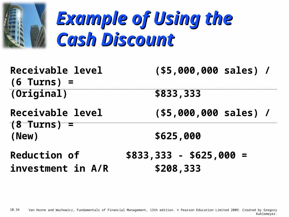
Receivable level ($5,000,000 sales) / (6 Turns) =(Original) $833,333

Receivable level ($5,000,000 sales) / (8 Turns) =(New) $625,000

Reduction of $833,333 - $625,000 =investment in A/R $208,333

Example of Using Example of Using the Cash Discountthe Cash Discount


Pre-tax cost of 0.02 x 0.3 x $5,000,000 =the cash discount $30,000$30,000..

Pre-tax opp. savings (20% opp. cost) x $208,333 =on reduction in A/R $41,667$41,667..

Yes! Yes! Savings > Costs

The benefits derived from released accounts receivable exceed the costs of providing the

discount to the firm’s customers.

Example of Using the Example of Using the Cash DiscountCash Discount


• Avoids carrying excess inventory and the associated carrying costs.

• Accept dating if warehousing costs plus the required return on investment in inventory exceeds the required return on additional receivables.

Seasonal DatingSeasonal Dating – Credit terms that encourage the buyer of seasonal products

to take delivery before the peak sales period and to defer payment until after the peak

sales period.

Seasonal DatingSeasonal Dating



(2) Bad-debtLosses




FirmFirmCollectionCollectionProgramProgram



PresentPolicy Policy A Policy B

Demand $2,400,000 $3,000,000 $3,300,000 Incremental sales $ 600,000 $ 300,000 Default losses Original sales 2% Incremental Sales 10% 18% Avg. Collection Pd. Original sales 1 month Incremental Sales 12 times 2 months 3 months

per year 6 times 4 times

Default Risk and Bad-Default Risk and Bad-Debt Losses Debt Losses (see p. 251 for details)(see p. 251 for details)


Policy A Policy B

1. Additional sales $600,000 $300,000 2. Profitability: (20% contribution) x (1)2. Profitability: (20% contribution) x (1) 120,000 120,000 60,000 60,000 3. Add. bad-debt losses: (1) x (bad-debt %) 60,000 54,000 4. Add. receivables: (1) / (New Rec. Turns) 100,000 75,000 5. Inv. in add. receivables: (.80) x (4) 80,000 60,000 6. Required before-tax return on

additional investment: (5) x (20%) 16,000 12,000 7. Additional bad-debt losses +7. Additional bad-debt losses +

additional required return: (3) + (6)additional required return: (3) + (6) 76,000 76,000 66,000 66,000

8. Incremental profitability: (2) - (7)8. Incremental profitability: (2) - (7) 44,000 44,000 (6,000) (6,000)

Adopt Policy A but not Policy B.Adopt Policy A but not Policy B.

Default Risk and Default Risk and Bad-Debt LossesBad-Debt Losses


The firm should increase collection expenditures collection expenditures until the marginal reduction in bad-debt losses bad-debt losses equals the marginal outlay to collect.

As an account becomes more overdue, the collection effort becomes more personal and more intense, until a resolution achieved.

Collection Collection Procedures Procedures

• Letters

• Phone calls

• Personal visits

• Legal action

SaturationSaturationPointPoint

Collection ExpendituresCollection Expenditures

Bad

-Deb

t L

oss

esB

ad-D

ebt

Lo

sses

Collection Policy Collection Policy and Proceduresand Procedures


• Obtaining information on the credit applicant

• Analyzing this information to determine the applicant’s creditworthiness

• Making the credit decision

Analyzing the Analyzing the Credit ApplicantCredit Applicant


• Financial statements• Credit ratings and reports• Bank checking• Trade checking• Company’s own experience

The company must weigh the amount amount of information of information needed versus the time time

and expense requiredand expense required.

Sources of InformationSources of Information


• the financial statements of the firm (ratio analysis)

• the character of the company• the character of management• the financial strength of the firm• other individual issues specific to

the firm

A credit analyst is likely to utilize A credit analyst is likely to utilize information regardinginformation regarding::

Credit AnalysisCredit Analysis


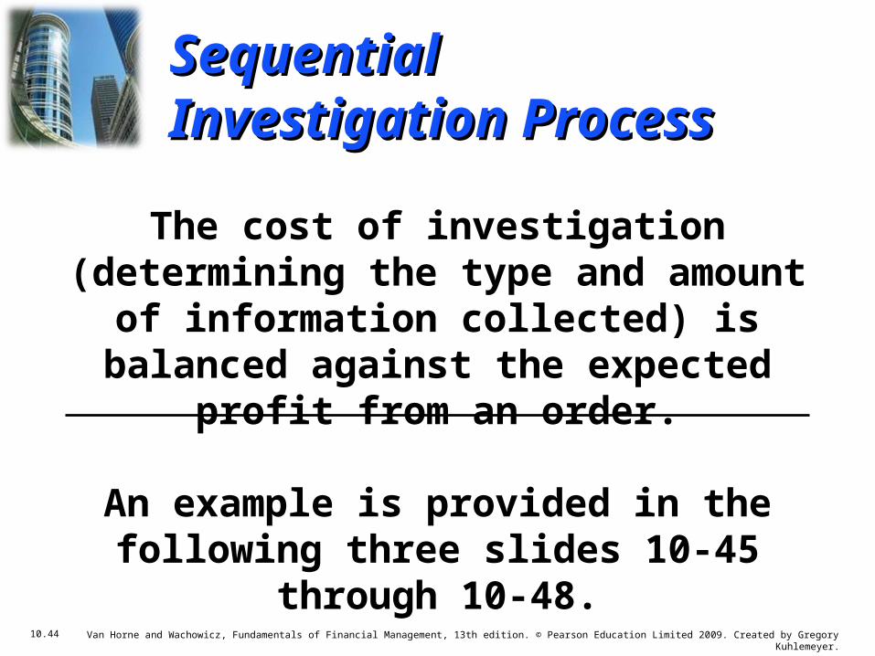
The cost of investigation (determining the type and amount of information collected) is balanced against the

expected profit from an order.

An example is provided in the following three slides 10-45 through 10-48.

Sequential Sequential Investigation ProcessInvestigation Process


* For previous customers only a Dun & Bradstreet reference book check.

Pending Order

Badpast creditexperience

Dun & Bradstreetreport analysis*

RejectYesNoStage 1$5 Cost

Stage 2$5 - $15

Cost

No prior experience whatsoever

Sample Investigation Sample Investigation Process Flow Chart (Part A)Process Flow Chart (Part A)


Accept

Yes

No

Credit rating“limited” and/or otherdamaging information

unearthed?

No

Yes

Reject

Credit rating“fair” and/or otherclose to maximum

“line of credit”?

Sample Investigation Sample Investigation Process Flow Chart (Part B)Process Flow Chart (Part B)


** That is, the credit of a bank is substituted for customer’s credit.

Bank, creditor, and financialstatement analysis

Accept RejectAccept, only upon

domestic irrevocableletter of credit (L/C)**

Fair PoorGood

Stage 3$30 Cost

Sample Investigation Sample Investigation Process Flow Chart (Part C)Process Flow Chart (Part C)


Line of CreditLine of Credit – A limit to the amount of credit extended to an account. Purchaser can buy on

credit up to that limit.

• Streamlines the procedure for shipping goods.

Credit-scoring SystemCredit-scoring System – A system used to decide whether to grant credit by assigning numerical scores to various characteristics

related to creditworthiness.

Other Credit Other Credit Decision IssuesDecision Issues


• Credit decisions are made• Ledger accounts maintained• Payments processed• Collections initiated

Decision based on the core competencies of the firm.

Outsourcing Credit and CollectionsOutsourcing Credit and Collections

The entire credit and/or collection function(s) are outsourced to a third-party company.

Other Credit Other Credit Decision IssuesDecision Issues


• Raw-materials inventory• Work-in-process inventory• In-transit inventory• Finished-goods inventory

Inventories form a link between production and sale of a product.

Inventory types:Inventory types:

Inventory Inventory Management and ControlManagement and Control


Inventory Management

Different areas will have differing perspectives in relation to inventory management which will be reflective of their own area’s objectives: Financial Manager: Keep stock as low as possible. Marketing Manager: Keep stock of finished goods

high. Manufacturing Manager: Keep raw materials

supplies high, and have large production runs. Purchasing Manager: Keep raw materials supplies

high.


• Purchasing• Production scheduling• Efficient servicing of customer

demands

Inventories provide flexibility Inventories provide flexibility for the firm in:for the firm in:

Inventory Inventory Management and ControlManagement and Control


Employ a cost-benefit analysisEmploy a cost-benefit analysis

Compare the benefits of economies of production, purchasing, and product

marketing against the cost of the additional investment in inventories.

How does a firm determine How does a firm determine the appropriate level of the appropriate level of

inventories?inventories?

Appropriate Appropriate Level of InventoriesLevel of Inventories


Method which controls expensive inventory

items more closely than less expensive items.

• Review “A” items most frequently

• Review “B” and “C” items less rigorously and/or less frequently.

ABC method of ABC method of inventory controlinventory control

0 15 45 1000 15 45 100

Cumulative Percentage Cumulative Percentage of Items in Inventoryof Items in Inventory

7070

9090

100100

Cu

mu

lati

ve P

erce

nta

ge

Cu

mu

lati

ve P

erce

nta

ge

of

Inve

nto

ry V

alu

eo

f In

ven

tory

Val

ue

AA

BBCC

ABC Method of ABC Method of Inventory ControlInventory Control



ABC System: Divides inventory into three categories A, B, & C

in descending order of importance and level of inventory, based on the dollar investment in each. A – The group requiring the largest dollar

investment, generally 20% of the firm’s inventory items which account for 80% of the firm’s dollar investment in inventory.

Monitored intensively and tracked using a perpetual inventory system to allow for daily verification of stock levels.



B – The middle group. Inventory levels are monitored through periodic checks.

C – The group of large numbers of inventory items, accounting for a relatively small amount of the investment in inventory.

Generally monitored using unsophisticated techniques such as the two bin method.


Economic Order QuantityEconomic Order Quantity

Determines an inventory item’s optimal order quantity that will reduce total inventory costs.

Achieved by minimising both the total of its order costs and carrying costs. Order Costs: The costs attributable to

placing and receiving an order. Carrying Costs: The cost per unit of

holding an item of inventory for a specific period of time.


Forecast usage Ordering cost Carrying cost

Ordering can mean either the purchase or Ordering can mean either the purchase or production of the item.production of the item.

The optimal quantity to order The optimal quantity to order depends on:depends on:

How Much to Order?How Much to Order?


CC: Carrying costs per unit per periodOO: Ordering costs per orderSS: Total usage during the periodQ: Order quantity in units

Total inventory costs (T) =Total inventory costs (T) =CC ( (Q / 2Q / 2) + ) + OO ( (SS / / QQ))

TIMETIME

Q / 2Q / 2

QQAverageAverage

InventoryInventory

INV

EN

TO

RY

IN

VE

NT

OR

Y

(in

un

its)

(in

un

its)

Total Inventory CostsTotal Inventory Costs


The EOQ or optimal quantity (Q*) is:

The quantity of an inventory item to order so that total inventory costs are minimized

over the firm’s planning period.

Q* Q* ==2 (2 (O) () (SS))

CC



Basket Wonders Basket Wonders is attempting to determine the economic order quantity for fabric used in the

production of baskets. • 10,000 yards of fabric were used at a constant

rate last period.• Each order represents an ordering cost of $200.• Carrying costs are $1 per yard over the 100-day

planning period.

What is the economic order quantity?What is the economic order quantity?

Example of the Example of the Economic Order QuantityEconomic Order Quantity


We will solve for the economic order quantity given that ordering costs are $200 per order, total usage over the period was 10,000 units,

and carrying costs are $1 per yard (unit).

Q* Q* ==2 (2 ($200) () (10,00010,000))

$1$1

Q* Q* = = 2,000 Units2,000 Units



EOQ (Q*) represents the minimum EOQ (Q*) represents the minimum point in total inventory costs.point in total inventory costs.


Total Carrying CostsTotal Carrying Costs

Total Ordering CostsTotal Ordering Costs

Q*Q* Order Size (Q)Order Size (Q)

Co

sts

Co

sts



Order PointOrder Point – The quantity to which inventory must fall in order to signal that an order must

be placed to replenish an item.

Order Point Order Point (OPOP) = Lead time Lead time X Daily usage

Issues to considerIssues to consider::Lead TimeLead Time – The length of time between the

placement of an order for an inventory item and when the item is received in inventory.

When to Order?When to Order?


Julie Miller of Basket Wonders Basket Wonders has determined that it takes only 2 days to receive the order of

fabric after the placement of the order.

When should Julie order more fabric?When should Julie order more fabric?

Lead time Lead time = = 2 days2 days

Daily usage Daily usage = 10,000 yards / 100 days = 10,000 yards / 100 days = = 100 yards per day100 yards per day

Order PointOrder Point = = 2 days 2 days xx 100 yards per day100 yards per day== 200 yards200 yards

Example of When to OrderExample of When to Order


0 0 18 20 38 40 18 20 38 40LeadLeadTimeTime

200200

20002000

OrderOrderPointPointU

NIT

SU

NIT

S

DAYSDAYS

Economic Order Quantity (Q*)Economic Order Quantity (Q*)

Example of When to OrderExample of When to Order


Our previous example assumed certain demand and lead time. When demand and/or lead time are

uncertain, then the order point is:

Order PointOrder Point =

(Avg. lead time x Avg. daily usage) + Safety stockSafety stock

Safety StockSafety Stock – Inventory stock held in reserve as a cushion against uncertain demand (or

usage) and replenishment lead time.

Safety StockSafety Stock


0 18 20 380 18 20 38

400400

20002000

OrderOrderPointPoint

UN

ITS

UN

ITS

DAYSDAYS

22002200

Safety StockSafety Stock200200

Order Point Order Point with Safety Stockwith Safety Stock


UN

ITS

UN

ITS

DAYSDAYS

Safety StockSafety Stock

Actual leadActual leadtime is 3 days!time is 3 days!

(at day 21)(at day 21)

22002200

20002000

OrderOrderPointPoint

400400

200200

0 18 210 18 21

The firm “dips”The firm “dips”into the safety stockinto the safety stock

Order Point Order Point with Safety Stockwith Safety Stock


• Amount of uncertainty in inventory demand

• Amount of uncertainty in the lead time

• Cost of running out of inventory

• Cost of carrying inventory

What is the proper amount of What is the proper amount of safety stock?safety stock?

Depends on theDepends on the::

How Much Safety Stock?How Much Safety Stock?


Just-in-TimeJust-in-Time

An inventory management system used to minimise inventory investment by having materials inputs arrive at exactly the time they are needed for production.

Carries little or no safety stocks. Relies on exceptional coordination between

firm, suppliers and logistics. Runs the risk of stalling production if

inventory fails to arrive when planned for.


Just-in-TimeJust-in-Time

Requirements of applying this Requirements of applying this approachapproach::

• A very accurate production and inventory information system

• Highly efficient purchasing• Reliable suppliers• Efficient inventory-handling system


EOQ and JIT example

Li Hong Company has an A group inventory item that is vital to the production process. This item costs $1,500, and Li Hong uses 1,100 units of the item per year. Li Hong wants to determine its optimal order strategy for the item. To calculate the EOQ, we need the following inputs:

Order cost per order = $150 Carrying cost per unit per year = $200 Substituting into EOQ Equation, we get EOQ =√(2 × 1,100 × $150)/200 ≈ 41 units


EOQ and JIT example

The reorder point depends on the number of days Li Hong operates per year. Assuming that he operates 250 days per year and uses 1,100 units of this item, its daily usage is 4.4 units (1,100 250).

If its lead time is two days and Li Hong wants to maintain a safety stock of four units, the reorder point for this item is 12.8 units ((2 × 4.4) + 4). However, orders are made only in whole units, so the order is placed when the inventory falls to 13 units.


EOQ and JIT example

Now assume the same information as before, but assume that the marginal cost of placing an order is (1) $11 or (2) $2.

1 Order cost of $11 EOQ = √(2 × 1,100 × $11)/200 = √121 = 11 units 2 Order cost of $2 EOQ = √(2 × 1,100 × $2)/200 = √22 = 5 units


EOQ and JIT example

As the order cost falls, the EOQ model now tells Li Hong to order fewer units per order, more often.

Applying a marginal order cost, the EOQ model moves towards a JIT system, where inventory arrives when it is needed, with an order cost based on the cost of a phone call to the supplier or a predetermined delivery schedule.

A pure JIT system assumes that suppliers will deliver on time, every time. Without such assurances, pure JIT systems can cause headaches for manufacturers


• JIT inventory control is one link in SCM.• The internet has enhanced SCM and

allows for many business-to-business (B2B) transactions

• Competition through B2B auctions helps reduce firm costs – especially standardized items

Supply Chain Management (SCM)Supply Chain Management (SCM) – Managing the process of moving goods, services, and

information from suppliers to end customers.

Supply Chain ManagementSupply Chain Management

10.1 Van Horne and Wachowicz, Fundamentals of Financial Management, 13th edition. © Pearson...

Documents

Transcript of 10.1 Van Horne and Wachowicz, Fundamentals of Financial Management, 13th edition. © Pearson...