The Gaussian (Normal) Distribution: More Details & Some Applications.

10: The Normal (Gaussian) DistributionLisa Yan
April 27, 2020
1

Lisa Yan, CS109, 2020
Quick slide reference
2
3 Normal RV 10a_normal
15 Normal RV: Properties 10b_normal_props
21 Normal RV: Computing probability 10c_normal_prob
30 Exercises LIVE

Normal RV
3
10a_normal

Lisa Yan, CS109, 2020
Today’s the Big Day
4
Today
Lisa Yan, CS109, 2020
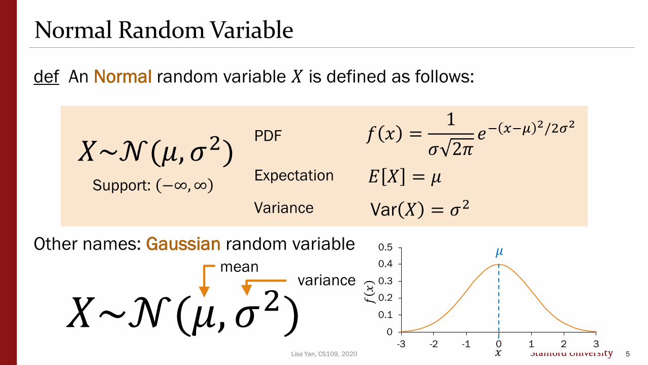
def An Normal random variable 𝑋 is defined as follows:
Other names: Gaussian random variable
Normal Random Variable
5
𝑓 𝑥 =1
𝜎 2𝜋𝑒− 𝑥−𝜇 2/2𝜎2
𝑋~𝒩(𝜇, 𝜎2)Support: −∞,∞
Variance
Expectation
𝐸 𝑋 = 𝜇
Var 𝑋 = 𝜎2
𝑋~𝒩(𝜇, 𝜎2)mean
variance
𝑥
𝑓𝑥

Lisa Yan, CS109, 2020
Carl Friedrich Gauss
Carl Friedrich Gauss (1777-1855) was a remarkably influentialGerman mathematician.
Did not invent Normal distribution but rather popularized it6

Lisa Yan, CS109, 2020
Why the Normal?
• Common for natural phenomena: height, weight, etc.
• Most noise in the world is Normal
• Often results from the sum of many random variables
• Sample means are distributed normally
7
That’s what they
want you to believe…

Lisa Yan, CS109, 2020
Why the Normal?
• Common for natural phenomena: height, weight, etc.
• Most noise in the world is Normal
• Often results from the sum of many random variables
• Sample means are distributed normally
8
Actually log-normal
Just an assumption
Only if equally weighted
(okay this one is true, we’ll see
this in 3 weeks)
Lisa Yan, CS109, 2020
0
0.05
0.1
0.15
0.2
0.25
0 … 44 48 52 56 60 64 … 900 … 44 48 52 56 60 64 … 90
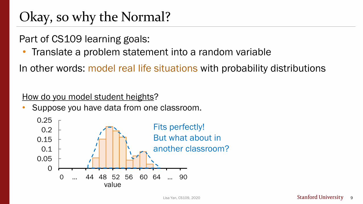
Okay, so why the Normal?
Part of CS109 learning goals:
• Translate a problem statement into a random variable
In other words: model real life situations with probability distributions
9
value
How do you model student heights?
• Suppose you have data from one classroom.
Fits perfectly!
But what about in
another classroom?

Lisa Yan, CS109, 2020
A Gaussian maximizes entropy for a
given mean and variance.
Part of CS109 learning goals:
• Translate a problem statement into a random variable
In other words: model real life situations with probability distributions
0
0.05
0.1
0.15
0.2
0.25
0 … 44 48 52 56 60 64 … 900 … 44 48 52 56 60 64 … 90
Okay, so why the Normal?
10
Occam’s Razor:
“Non sunt multiplicanda
entia sine necessitate.”
Entities should not be multiplied
without necessity.
value
How do you model student heights?
• Suppose you have data from one classroom.
• Same mean/var
• Generalizes well

Lisa Yan, CS109, 2020
I encourage you to stay critical of how
to model real-world phenomena.
Why the Normal?
• Common for natural phenomena: height, weight, etc.
• Most noise in the world is Normal
• Often results from the sum of many random variables
• Sample means are distributed normally
11
Actually log-normal
Just an assumption
Only if equally weighted
(okay this one is true, we’ll see
this in 3 weeks)

Lisa Yan, CS109, 2020
Anatomy of a beautiful equation
Let 𝑋~𝒩 𝜇, 𝜎2 .
The PDF of 𝑋 is defined as:
12
𝑓 𝑥 =1
𝜎 2𝜋𝑒−
𝑥 − 𝜇 2
2𝜎2
normalizing constantexponential
tail
symmetric
around 𝜇
variance 𝜎2
manages spread
𝑥
𝑓𝑥

Lisa Yan, CS109, 2020
Campus bikes
You spend some minutes, 𝑋, travelingbetween classes.
• Average time spent: 𝜇 = 4 minutes
• Variance of time spent: 𝜎2 = 2 minutes2
Suppose 𝑋 is normally distributed. What is the probability you spend ≥ 6 minutes traveling?
13
𝑋~𝒩(𝜇 = 4, 𝜎2 = 2)
𝑃 𝑋 ≥ 6 = න6
∞
𝑓(𝑥)𝑑𝑥 = න6
∞ 1
𝜎 2𝜋𝑒−
𝑥 − 𝜇 2
2𝜎2 𝑑𝑥
(call me if you analytically solve this)Loving, not scary…except this time

Lisa Yan, CS109, 2020
Computing probabilities with Normal RVs
For a Normal RV 𝑋~𝒩 𝜇, 𝜎2 , its CDF has no closed form.
𝑃 𝑋 ≤ 𝑥 = 𝐹 𝑥 = න−∞
𝑥 1
𝜎 2𝜋𝑒−
𝑦 − 𝜇 2
2𝜎2 𝑑𝑦
However, we can solve for probabilities numerically using a function Φ:
𝐹 𝑥 = Φ𝑥 − 𝜇
𝜎
14
Cannot be
solved
analytically
⚠️
CDF of
𝑋~𝒩 𝜇, 𝜎2A function that has been
solved for numerically
To get here, we’ll first
need to know some
properties of Normal RVs.

Normal RV: Properties
15
10b_normal_props

Lisa Yan, CS109, 2020
Properties of Normal RVs
Let 𝑋~𝒩 𝜇, 𝜎2 with CDF 𝑃 𝑋 ≤ 𝑥 = 𝐹 𝑥 .
1. Linear transformations of Normal RVs are also Normal RVs.
If 𝑌 = 𝑎𝑋 + 𝑏, then 𝑌~𝒩(𝑎𝜇 + 𝑏, 𝑎2𝜎2).
2. The PDF of a Normal RV is symmetric about the mean 𝜇.
𝐹 𝜇 − 𝑥 = 1 − 𝐹 𝜇 + 𝑥
16

Lisa Yan, CS109, 2020
1. Linear transformations of Normal RVs
Let 𝑋~𝒩 𝜇, 𝜎2 with CDF 𝑃 𝑋 ≤ 𝑥 = 𝐹 𝑥 .
Linear transformations of X are also Normal.
If 𝑌 = 𝑎𝑋 + 𝑏, then 𝑌~𝒩 𝑎𝜇 + 𝑏, 𝑎2𝜎2
Proof:
• 𝐸 𝑌 = 𝐸 𝑎𝑋 + 𝑏 = 𝑎𝐸 𝑋 + 𝑏 = 𝑎𝜇 + 𝑏
• Var 𝑌 = Var 𝑎𝑋 + 𝑏 = 𝑎2Var 𝑋 = 𝑎2𝜎2
• 𝑌 is also Normal
17
Proof in Ross,
10th ed (Section 5.4)
Linearity of Expectation
Var 𝑎𝑋 + 𝑏 = 𝑎2Var 𝑋

Lisa Yan, CS109, 2020
2. Symmetry of Normal RVs
Let 𝑋~𝒩 𝜇, 𝜎2 with CDF 𝑃 𝑋 ≤ 𝑥 = 𝐹 𝑥 .
The PDF of a Normal RV is symmetric about the mean 𝜇.
𝐹 𝜇 − 𝑥 = 1 − 𝐹 𝜇 + 𝑥
18
𝑓(𝑥)
𝑥𝜇

Lisa Yan, CS109, 2020
Using symmetry of the Normal RV
19
1. 𝑃 𝑍 ≤ 𝑧
2. 𝑃 𝑍 < 𝑧
3. 𝑃 𝑍 ≥ 𝑧
4. 𝑃 𝑍 ≤ −𝑧
5. 𝑃 𝑍 ≥ −𝑧
6. 𝑃(𝑦 < 𝑍 < 𝑧) 🤔
A. 𝐹 𝑧
B. 1 − 𝐹(𝑧)
C. 𝐹 𝑧 − 𝐹(𝑦)
= 𝐹 𝑧
𝑧
𝑓(𝑧)
𝐹 𝜇 − 𝑥 = 1 − 𝐹 𝜇 + 𝑥
𝜇 = 0
Let 𝑍~𝒩 0,1 with CDF 𝑃 𝑍 ≤ 𝑧 = 𝐹 𝑧 .
Suppose we only knew numeric valuesfor 𝐹 𝑧 and 𝐹 𝑦 , for some 𝑧, 𝑦 ≥ 0.
How do we compute the following probabilities?
Lisa Yan, CS109, 2020
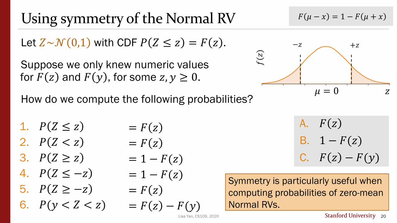
Using symmetry of the Normal RV
20
1. 𝑃 𝑍 ≤ 𝑧
2. 𝑃 𝑍 < 𝑧
3. 𝑃 𝑍 ≥ 𝑧
4. 𝑃 𝑍 ≤ −𝑧
5. 𝑃 𝑍 ≥ −𝑧
6. 𝑃(𝑦 < 𝑍 < 𝑧)
A. 𝐹 𝑧
B. 1 − 𝐹(𝑧)
C. 𝐹 𝑧 − 𝐹(𝑦)
= 𝐹 𝑧
= 𝐹 𝑧
= 1 − 𝐹(𝑧)
= 1 − 𝐹(𝑧)
= 𝐹 𝑧
= 𝐹 𝑧 − 𝐹(𝑦)
Symmetry is particularly useful when
computing probabilities of zero-mean
Normal RVs.
𝑧
𝑓(𝑧)
𝐹 𝜇 − 𝑥 = 1 − 𝐹 𝜇 + 𝑥
𝜇 = 0
Let 𝑍~𝒩 0,1 with CDF 𝑃 𝑍 ≤ 𝑧 = 𝐹 𝑧 .
Suppose we only knew numeric valuesfor 𝐹 𝑧 and 𝐹 𝑦 , for some 𝑧, 𝑦 ≥ 0.
How do we compute the following probabilities?

Normal RV:Computing probability
21
10c_normal_probs

Lisa Yan, CS109, 2020
Computing probabilities with Normal RVs
Let 𝑋~𝒩 𝜇, 𝜎2 .
To compute the CDF, 𝑃 𝑋 ≤ 𝑥 = 𝐹 𝑥 :
• We cannot analytically solve the integral (it has no closed form)
• …but we can solve numerically using a function Φ:
𝐹 𝑥 = Φ𝑥 − 𝜇
𝜎
22
CDF of the
Standard Normal, 𝑍

Lisa Yan, CS109, 2020
The Standard Normal random variable 𝑍 is defined as follows:
Other names: Unit Normal
CDF of 𝑍 defined as:
Standard Normal RV, 𝑍
23
𝑍~𝒩(0, 1) Variance
Expectation 𝐸 𝑍 = 𝜇 = 0
Var 𝑍 = 𝜎2 = 1
𝑃 𝑍 ≤ 𝑧 = Φ(𝑧)
Note: not a new distribution; just
a special case of the Normal
Lisa Yan, CS109, 2020
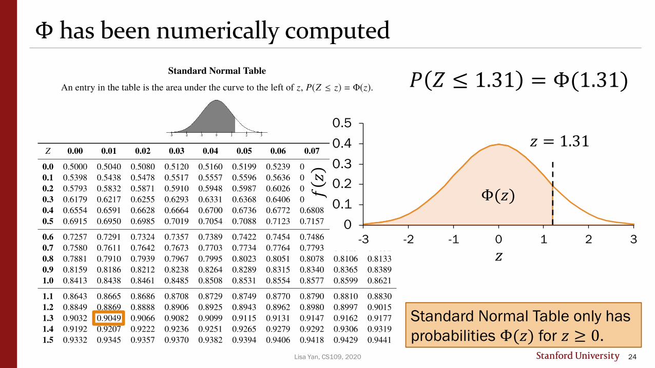
Φ has been numerically computed
24
𝑃 𝑍 ≤ 1.31 = Φ(1.31)
𝑓𝑧
𝑧
Φ(𝑧)
Standard Normal Table only has
probabilities Φ(𝑧) for 𝑧 ≥ 0.

Lisa Yan, CS109, 2020
History fact: Standard Normal Table
25
The first Standard Normal Table was computed by Christian Kramp, French astronomer (1760–1826), in Analysedes Réfractions Astronomiques et Terrestres, 1799
Used a Taylor series expansion to the third power
Lisa Yan, CS109, 2020
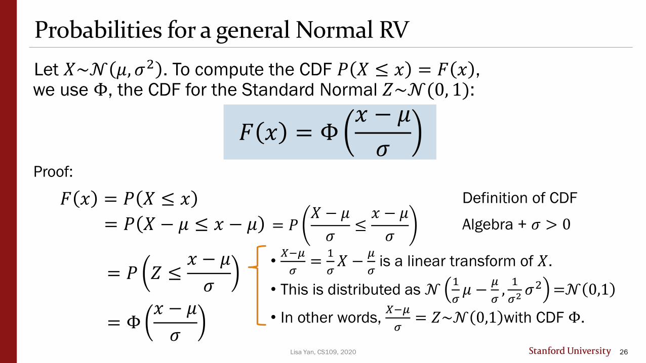
Probabilities for a general Normal RV
Let 𝑋~𝒩 𝜇, 𝜎2 . To compute the CDF 𝑃 𝑋 ≤ 𝑥 = 𝐹 𝑥 ,we use Φ, the CDF for the Standard Normal 𝑍~𝒩(0, 1):
𝐹 𝑥 = Φ𝑥 − 𝜇
𝜎Proof:
26
𝐹 𝑥 = 𝑃 𝑋 ≤ 𝑥
= 𝑃 𝑋 − 𝜇 ≤ 𝑥 − 𝜇 = 𝑃𝑋 − 𝜇
𝜎≤𝑥 − 𝜇
𝜎
= 𝑃 𝑍 ≤𝑥 − 𝜇
𝜎
Algebra + 𝜎 > 0
Definition of CDF
•𝑋−𝜇
𝜎=
1
𝜎𝑋 −
𝜇
𝜎is a linear transform of 𝑋.
• This is distributed as 𝒩1
𝜎𝜇 −
𝜇
𝜎,1
𝜎2𝜎2 =𝒩 0,1
• In other words, 𝑋−𝜇
𝜎= 𝑍~𝒩 0,1 with CDF Φ.= Φ
𝑥 − 𝜇
𝜎

Lisa Yan, CS109, 2020
Probabilities for a general Normal RV
Let 𝑋~𝒩 𝜇, 𝜎2 . To compute the CDF 𝑃 𝑋 ≤ 𝑥 = 𝐹 𝑥 ,we use Φ, the CDF for the Standard Normal 𝑍~𝒩(0, 1):
𝐹 𝑥 = Φ𝑥 − 𝜇
𝜎Proof:
27
𝐹 𝑥 = 𝑃 𝑋 ≤ 𝑥
= 𝑃 𝑋 − 𝜇 ≤ 𝑥 − 𝜇 = 𝑃𝑋 − 𝜇
𝜎≤𝑥 − 𝜇
𝜎
= 𝑃 𝑍 ≤𝑥 − 𝜇
𝜎
Algebra + 𝜎 > 0
Definition of CDF
•𝑋−𝜇
𝜎=
1
𝜎𝑋 −
𝜇
𝜎is a linear transform of 𝑋.
• This is distributed as 𝒩1
𝜎𝜇 −
𝜇
𝜎,1
𝜎2𝜎2 =𝒩 0,1
• In other words, 𝑋−𝜇
𝜎= 𝑍~𝒩 0,1 with CDF Φ.= Φ
𝑥 − 𝜇
𝜎
1. Compute 𝑧 = 𝑥 − 𝜇 /𝜎.
2. Look up Φ 𝑧 in Standard Normal table.

Lisa Yan, CS109, 2020
Campus bikes
You spend some minutes, 𝑋, traveling between classes.• Average time spent: 𝜇 = 4 minutes• Variance of time spent: 𝜎2 = 2 minutes2
Suppose 𝑋 is normally distributed. What is the probability you spend ≥ 6 minutes traveling?
28
𝑋~𝒩(𝜇 = 4, 𝜎2 = 2) 𝑃 𝑋 ≥ 6 = න6
∞
𝑓(𝑥)𝑑𝑥 (no analytic solution)
1. Compute 𝑧 =𝑥−𝜇
𝜎2. Look up Φ(𝑧) in table
𝑃 𝑋 ≥ 6 = 1 − 𝐹𝑥(6)
= 1 − Φ6 − 4
2
×
≈ 1 − Φ 1.41
1 − Φ 1.41≈ 1 − 0.9207= 0.0793

Lisa Yan, CS109, 2020
Is there an easier way? (yes)
Let 𝑋~𝒩 𝜇, 𝜎2 . What is 𝑃 𝑋 ≤ 𝑥 = 𝐹 𝑥 ?
• Use Python
• Use website tool
29
from scipy import statsX = stats.norm(mu, std)X.cdf(x)
SciPy reference:https://docs.scipy.org/doc/scipy/refere
nce/generated/scipy.stats.norm.html
Website tool: https://web.stanford.edu/class/cs109
/handouts/normalCDF.html

(live)10: The Normal (Gaussian) DistributionLisa Yan
July 13, 2020
30

Lisa Yan, CS109, 2020
The Normal (Gaussian) Random Variable
Let 𝑋~𝒩 𝜇, 𝜎2 .
The PDF of 𝑋 is defined as:
31
𝑓 𝑥 =1
𝜎 2𝜋𝑒−
𝑥 − 𝜇 2
2𝜎2
normalizing constantexponential
tail
symmetric
around 𝜇
variance 𝜎2
manages spread
𝑥
𝑓𝑥
Review

ThinkSlide 34 has a question to go over by yourself.
Post any clarifications here!
https://us.edstem.org/courses/667/discussion/89934
Think by yourself: 2 min
32
🤔(by yourself)

Lisa Yan, CS109, 2020
Normal Random Variable
Match PDF to distribution:
𝒩 0, 1
𝒩(−2, 0.5)
𝒩 0, 5
𝒩(0, 0.2)
33
A.
B.
C.
D.
𝑋~𝒩(𝜇, 𝜎2)mean variance
🤔(by yourself)
𝑥
𝑓𝑥

Lisa Yan, CS109, 2020
Knowing how to use a Standard Normal Table will
still be useful in our understanding of Normal RVs.
Computing probabilities with Normal RVs: Old school
34
*particularly useful if we had closed book exams with no calculator**
**we have open book exams with calculators this quarter
Φ 𝑧 for non-negative 𝑧
*
Lisa Yan, CS109, 2020
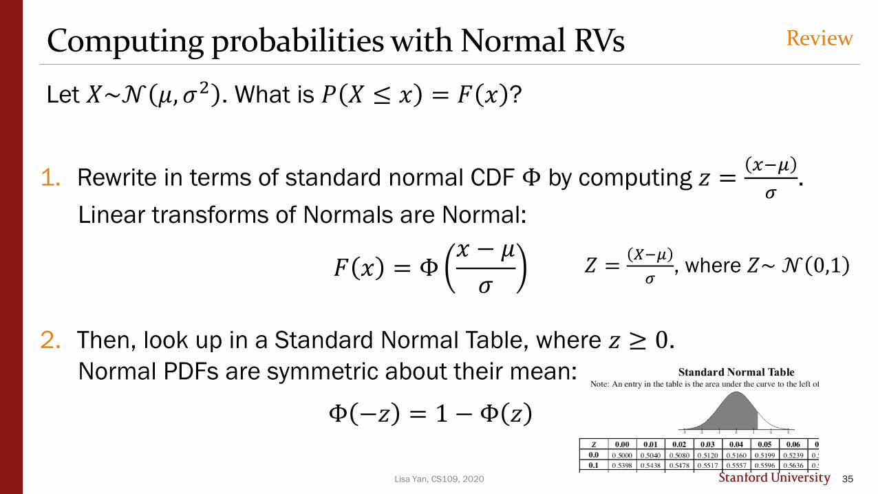
Computing probabilities with Normal RVs
Let 𝑋~𝒩 𝜇, 𝜎2 . What is 𝑃 𝑋 ≤ 𝑥 = 𝐹 𝑥 ?
1. Rewrite in terms of standard normal CDF Φ by computing 𝑧 =𝑥−𝜇
𝜎.
Linear transforms of Normals are Normal:
𝐹 𝑥 = Φ𝑥 − 𝜇
𝜎
2. Then, look up in a Standard Normal Table, where 𝑧 ≥ 0.
Normal PDFs are symmetric about their mean:
Φ −𝑧 = 1 − Φ 𝑧
35
Review
𝑍 =𝑋−𝜇
𝜎, where 𝑍~ 𝒩 0,1

Lisa Yan, CS109, 2020
Get your Gaussian On
Let 𝑋~𝒩 𝜇 = 3, 𝜎2 = 16 . Std deviation 𝜎 = 4.
1. 𝑃 𝑋 > 0
36
• If 𝑋~𝒩 𝜇, 𝜎2 , then
𝐹 𝑥 = Φ𝑥−𝜇
𝜎
• Symmetry of the PDF of
Normal RV implies
Φ −𝑧 = 1 − Φ 𝑧

Breakout Rooms
Slide 39 has two questions to go over in groups.
Post any clarifications here!
https://us.edstem.org/courses/667/discussion/89934
Breakout rooms: 5 mins
37
🤔

Lisa Yan, CS109, 2020
Get your Gaussian On
Let 𝑋~𝒩 𝜇 = 3, 𝜎2 = 16 .Note standard deviation 𝜎 = 4.
How would you write each of the belowprobabilities as a function of thestandard normal CDF, Φ?
1. 𝑃 𝑋 > 0 (we just did this)
2. 𝑃 2 < 𝑋 < 5
3. 𝑃 𝑋 − 3 > 6
38
• If 𝑋~𝒩 𝜇, 𝜎2 , then
𝐹 𝑥 = Φ𝑥−𝜇
𝜎
• Symmetry of the PDF of
Normal RV implies
Φ −𝑧 = 1 − Φ 𝑧
🤔

Lisa Yan, CS109, 2020
Get your Gaussian On
Let 𝑋~𝒩 𝜇 = 3, 𝜎2 = 16 . Std deviation 𝜎 = 4.
1. 𝑃 𝑋 > 0
2. 𝑃 2 < 𝑋 < 5
39
• If 𝑋~𝒩 𝜇, 𝜎2 , then
𝐹 𝑥 = Φ𝑥−𝜇
𝜎
• Symmetry of the PDF of
Normal RV implies
Φ −𝑧 = 1 − Φ 𝑧

Lisa Yan, CS109, 2020
Get your Gaussian On
Let 𝑋~𝒩 𝜇 = 3, 𝜎2 = 16 . Std deviation 𝜎 = 4.
1. 𝑃 𝑋 > 0
2. 𝑃 2 < 𝑋 < 5
3. 𝑃 𝑋 − 3 > 6
40
Compute 𝑧 =𝑥−𝜇
𝜎
• If 𝑋~𝒩 𝜇, 𝜎2 , then
𝐹 𝑥 = Φ𝑥−𝜇
𝜎
• Symmetry of the PDF of
Normal RV implies
Φ −𝑥 = 1 − Φ 𝑥
𝑃 𝑋 < −3 + 𝑃 𝑋 > 9
= 𝐹 −3 + 1 − 𝐹 9
= Φ−3 − 3
4+ 1 −Φ
9 − 3
4
Look up Φ(z) in table

Lisa Yan, CS109, 2020
Get your Gaussian On
Let 𝑋~𝒩 𝜇 = 3, 𝜎2 = 16 . Std deviation 𝜎 = 4.
1. 𝑃 𝑋 > 0
2. 𝑃 2 < 𝑋 < 5
3. 𝑃 𝑋 − 3 > 6
41
Compute z =𝑥−𝜇
𝜎Look up Φ(z) in table
𝑃 𝑋 < −3 + 𝑃 𝑋 > 9
= 𝐹 −3 + 1 − 𝐹 9
= Φ−3 − 3
4+ 1 −Φ
9 − 3
4
= Φ −3
2+ 1 −Φ
3
2
= 2 1 − Φ3
2
≈ 0.1337
• If 𝑋~𝒩 𝜇, 𝜎2 , then
𝐹 𝑥 = Φ𝑥−𝜇
𝜎
• Symmetry of the PDF of
Normal RV implies
Φ −𝑥 = 1 − Φ 𝑥

Interlude for jokes/announcements
42

Lisa Yan, CS109, 2020
Announcements
43
Problem Set 3
Due: Friday 7/13 1pm PT
Tim’s OH permanently moved to 8-10pm PT, Wednesday

Lisa Yan, CS109, 2020
Interesting probability news
44
https://www.forbes.com/sites/lanceeliot/2020/04/12/on-
the-probabilities-of-social-distancing-as-gleaned-from-ai-self-
driving-cars/#218da4489472

Breakout Rooms
Slide 47 has two questions to go over in groups.
Post any clarifications here!
https://us.edstem.org/courses/667/discussion/89934
Breakout rooms: 5 mins
45
🤔

Lisa Yan, CS109, 2020
Noisy Wires
Send a voltage of 2 V or −2 V onwire (to denote 1 and 0, respectively).
• 𝑋 = voltage sent (2 or −2)• 𝑌 = noise, 𝑌~𝒩 0, 1• 𝑅 = 𝑋 + 𝑌 voltage received.
Decode: 1 if 𝑅 ≥ 0.50 otherwise.
1. What is P(decoding error | original bit is 1)?i.e., we sent 1, but we decoded as 0?
2. What is P(decoding error | original bit is 0)?
These probabilities are unequal. Why might this be useful?46
🤔𝐹𝑅(𝑟)
𝑅 = 𝑟

Lisa Yan, CS109, 2020
Noisy Wires
Send a voltage of 2 V or −2 V onwire (to denote 1 and 0, respectively).
• 𝑋 = voltage sent (2 or −2)• 𝑌 = noise, 𝑌~𝒩 0, 1• 𝑅 = 𝑋 + 𝑌 voltage received.
Decode: 1 if 𝑅 ≥ 0.50 otherwise.
1. What is P(decoding error | original bit is 1)?i.e., we sent 1, but we decoded as 0?
47𝐹𝑅(𝑟)
𝑅 = 𝑟
𝑃 𝑅 < 0.5| 𝑋 = 2 = 𝑃 2 + 𝑌 < 0.5 = 𝑃 𝑌 < −1.5 Y is Standard Normal
= Φ −1.5 = 1 − Φ 1.5 ≈ 0.0668
Lisa Yan, CS109, 2020
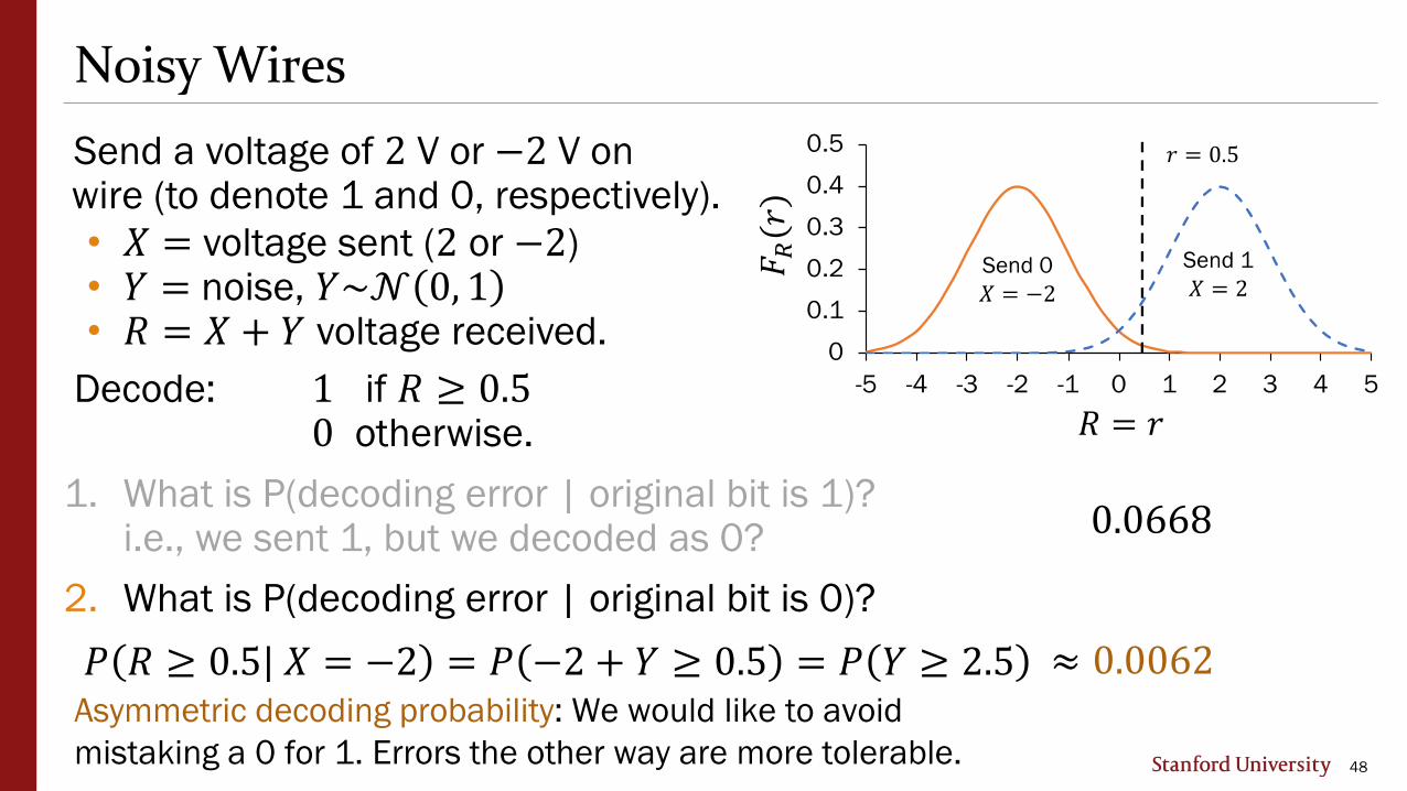
Noisy Wires
Send a voltage of 2 V or −2 V onwire (to denote 1 and 0, respectively).
• 𝑋 = voltage sent (2 or −2)• 𝑌 = noise, 𝑌~𝒩 0, 1• 𝑅 = 𝑋 + 𝑌 voltage received.
Decode: 1 if 𝑅 ≥ 0.50 otherwise.
1. What is P(decoding error | original bit is 1)?i.e., we sent 1, but we decoded as 0?
2. What is P(decoding error | original bit is 0)?
48𝐹𝑅(𝑟)
𝑅 = 𝑟
0.0668
≈ 0.0062𝑃 𝑅 ≥ 0.5| 𝑋 = −2 = 𝑃 −2 + 𝑌 ≥ 0.5 = 𝑃 𝑌 ≥ 2.5Asymmetric decoding probability: We would like to avoid
mistaking a 0 for 1. Errors the other way are more tolerable.

Challenge: Sampling with the Normal RV
49
LIVE

Lisa Yan, CS109, 2020
ELO ratings
50
What is the probability that the Warriors win?
How do you model zero-sum games?

Lisa Yan, CS109, 2020
ELO ratings
Each team has an ELO score 𝑆, calculated based on theirpast performance.
• Each game, a team hasability 𝐴~𝒩 𝑆, 2002 .
• The team with the highersampled ability wins.
What is the probabilitythat Warriors winthis game?
Want: 𝑃 Warriors win = 𝑃 𝐴𝑊 > 𝐴𝐵
51
0
0.0005
0.001
0.0015
0.002
0.0025
1000 1500 2000 2500
𝜇=1470
0
0.0005
0.001
0.0015
0.002
0.0025
1000 1500 2000 2500
𝜇=1657
Arpad Elo
Warriors 𝐴𝑊~𝒩 𝑆 = 1657, 2002
Opponents 𝐴𝐵~𝒩 𝑆 = 1470, 2002

Lisa Yan, CS109, 2020
ELO ratings
52
Want: 𝑃 Warriors win = 𝑃 𝐴𝑊 > 𝐴𝐵
≈ 0.7488, calculated by sampling
from scipy import statsWARRIORS_ELO = 1657OPPONENT_ELO = 1470STDEV = 200NTRIALS = 10000
nSuccess = 0for i in range(NTRIALS):w = stats.norm.rvs(WARRIORS_ELO, STDEV)b = stats.norm.rvs(OPPONENT_ELO, STDEV)if w > b:nSuccess += 1
print("Warriors sampled win fraction", float(nSuccess) /NTRIALS)

Lisa Yan, CS109, 2020
Is there a better way?
𝑃 𝐴𝑊 > 𝐴𝐵
• This is a probability of an event involving two random variables!
• We’ll solve this problem analytically in upcoming weeks.
Big goal for next time: Events involving two discrete random variables.Stay tuned!
53