1. Welding, Bonding, and the Design of Permanent Joints

Form can more readily pursue function with the help of joining

processes such as welding, brazing, soldering, cementing, and

gluing–processes that are used extensively in manufacturing today.

Whenever parts have to be assembled or fabricated, there is usually

good cause for considering one of these processes in preliminary

design work. Particularly when sections to be joined are thin, one of

these methods may lead to significant savings. The elimination of

individual fasteners, with their holes and assembly costs, is an

important factor. Also, some of the methods allow rapid machine

assembly, furthering their attractiveness.

6.1 Welding Symbols

A weldment is fabricated by welding together a collection of metal

shapes, cut to particular configurations. During welding, the several

parts are held securely together, often by clamping or jigging. The

welds must be precisely specified on working drawings, and this is

done by using the welding symbol, shown in Fig. (6–1), as

standardized by the American Welding Society (AWS). The arrow

of this symbol points to the joint to be welded. The body of the

symbol contains as many of the following elements as are deemed

necessary:

• Reference line

• Arrow

• Basic weld symbols as in Fig. (6–2)

• Dimensions and other data

• Supplementary symbols

• Finish symbols

• Tail

• Specification or process

The arrow side of a joint is the line, side, area, or near member to

which the arrow points. The side opposite the arrow side is the other

side.

Figures (6–3 to 6–6) illustrate the types of welds used most

frequently by designers. For general machine elements most welds

are fillet welds, though butt welds are used a great deal in designing

pressure vessels. Of course, the parts to be joined must be arranged

so that there is sufficient clearance for the welding operation. If

unusual joints are required because of insufficient clearance or

because of the section shape, the design may be a poor one and the

designer should begin again and endeavor to synthesize another

solution.

Figure (6–1) The AWS standard welding symbol showing the location

of the symbol elements

Figure (6–2) Arc- and gas-weld symbols

Figure (6–3) Fillet welds. (a) The number indicates the leg size; the arrow should point only

to one weld when both sides are the same. (b) The symbol indicates that the

welds are intermittent and staggered 60 mm along on 200-mm centers

Figure (6–4) The circle on the weld symbol

indicates that the welding is to

go all around

Figure (6–5) Butt or groove welds: (a) square butt-welded on both sides; (b) single V with

60° bevel and root opening of 2 mm; (c) double V; (d) single bevel

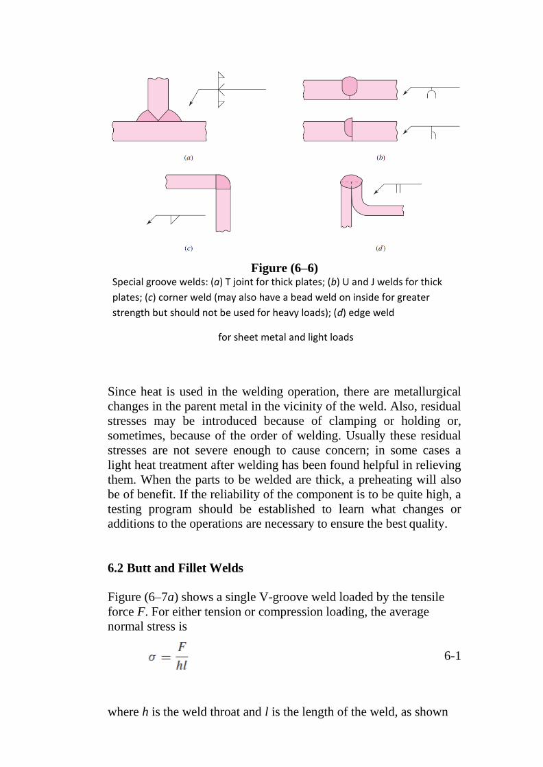
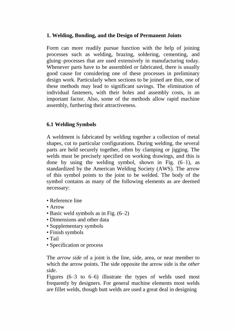
Figure (6–6) Special groove welds: (a) T joint for thick plates; (b) U and J welds for thick

plates; (c) corner weld (may also have a bead weld on inside for greater

strength but should not be used for heavy loads); (d) edge weld

for sheet metal and light loads

Since heat is used in the welding operation, there are metallurgical

changes in the parent metal in the vicinity of the weld. Also, residual

stresses may be introduced because of clamping or holding or,

sometimes, because of the order of welding. Usually these residual

stresses are not severe enough to cause concern; in some cases a

light heat treatment after welding has been found helpful in relieving

them. When the parts to be welded are thick, a preheating will also

be of benefit. If the reliability of the component is to be quite high, a

testing program should be established to learn what changes or

additions to the operations are necessary to ensure the best quality.

6.2 Butt and Fillet Welds

Figure (6–7a) shows a single V-groove weld loaded by the tensile

force F. For either tension or compression loading, the average

normal stress is

6-1

where h is the weld throat and l is the length of the weld, as shown

in the figure. Note that the value of h does not include the

reinforcement. The reinforcement can be desirable, but it varies

somewhat and does produce stress concentration at point A in the

figure. If fatigue loads exist, it is good practice to grind or machine

off the reinforcement.

Figure (6–7) A typical butt joint

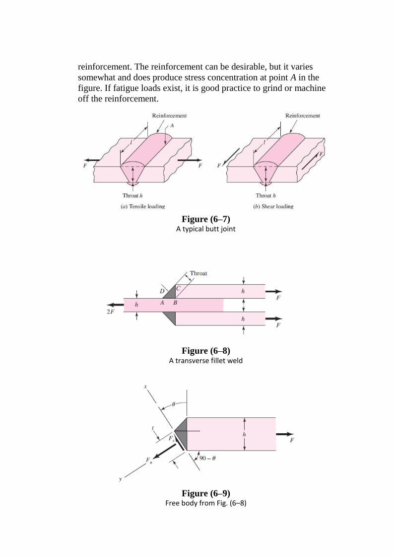
Figure (6–8) A transverse fillet weld

Figure (6–9) Free body from Fig. (6–8)

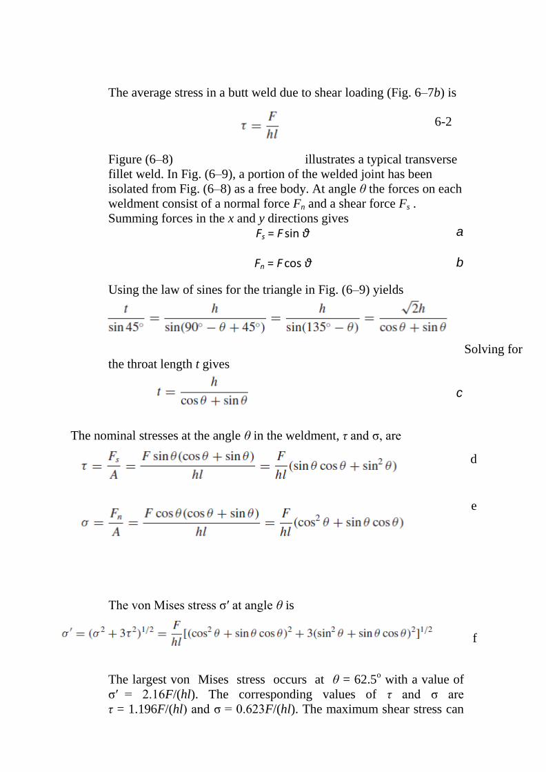
The average stress in a butt weld due to shear loading (Fig. 6–7b) is

6-2

Figure (6–8) illustrates a typical transverse

fillet weld. In Fig. (6–9), a portion of the welded joint has been

isolated from Fig. (6–8) as a free body. At angle θ the forces on each

weldment consist of a normal force Fn and a shear force Fs .

Summing forces in the x and y directions gives

Fs = F sin θ a

Fn = F cos θ b

Using the law of sines for the triangle in Fig. (6–9) yields

Solving for

the throat length t gives

The nominal stresses at the angle θ in the weldment, τ and σ, are

d

e

The von Mises stress σ′ at angle θ is

f

The largest von Mises stress occurs at θ = 62.5o with a value of

σ′ = 2.16F/(hl). The corresponding values of τ and σ are

τ = 1.196F/(hl) and σ = 0.623F/(hl). The maximum shear stress can

c

be found by differentiating Eq. (d) with respect to θ and equating to

zero. The stationary point occurs at θ = 67.5o with a corresponding

τmax = 1.207F/(hl) and σ = 0.5F/(hl).

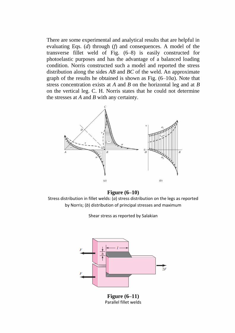
There are some experimental and analytical results that are helpful in

evaluating Eqs. (d) through (f) and consequences. A model of the

transverse fillet weld of Fig. (6–8) is easily constructed for

photoelastic purposes and has the advantage of a balanced loading

condition. Norris constructed such a model and reported the stress

distribution along the sides AB and BC of the weld. An approximate

graph of the results he obtained is shown as Fig. (6–10a). Note that

stress concentration exists at A and B on the horizontal leg and at B

on the vertical leg. C. H. Norris states that he could not determine

the stresses at A and B with any certainty.

Figure (6–10) Stress distribution in fillet welds: (a) stress distribution on the legs as reported

by Norris; (b) distribution of principal stresses and maximum

Shear stress as reported by Salakian

Figure (6–11) Parallel fillet welds

A. G. Salakian and G. E. Claussen presents data for the stress

distribution across the throat of a fillet weld (Fig. 6–10b). This graph

is of particular interest because we have just learned that it is the

throat stresses that are used in design. Again, the figure shows stress

concentration at point B. Note that Fig. (6–10a) applies either to the

weld metal or to the parent metal, and that Fig. (6–10b) applies only

to the weld metal. The most important concept here is that we have

no analytical approach that predicts the existing stresses. The

geometry of the fillet is crude by machinery standards, and even if it

were ideal, the macrogeometry is too abrupt and complex for our

methods. There are also subtle bending stresses due to eccentricities.

Still, in the absence of robust analysis, weldments must be specified

and the resulting joints must be safe. The approach has been to use a

simple and conservative model, verified by testing as conservative.

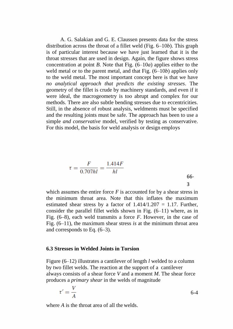
For this model, the basis for weld analysis or design employs

66-

3

which assumes the entire force F is accounted for by a shear stress in

the minimum throat area. Note that this inflates the maximum

estimated shear stress by a factor of 1.414/1.207 = 1.17. Further,

consider the parallel fillet welds shown in Fig. (6–11) where, as in

Fig. (6–8), each weld transmits a force F. However, in the case of

Fig. (6–11), the maximum shear stress is at the minimum throat area

and corresponds to Eq. (6–3).

6.3 Stresses in Welded Joints in Torsion

Figure (6–12) illustrates a cantilever of length l welded to a column

by two fillet welds. The reaction at the support of a cantilever

always consists of a shear force V and a moment M. The shear force

produces a primary shear in the welds of magnitude

6-4

where A is the throat area of all the welds.

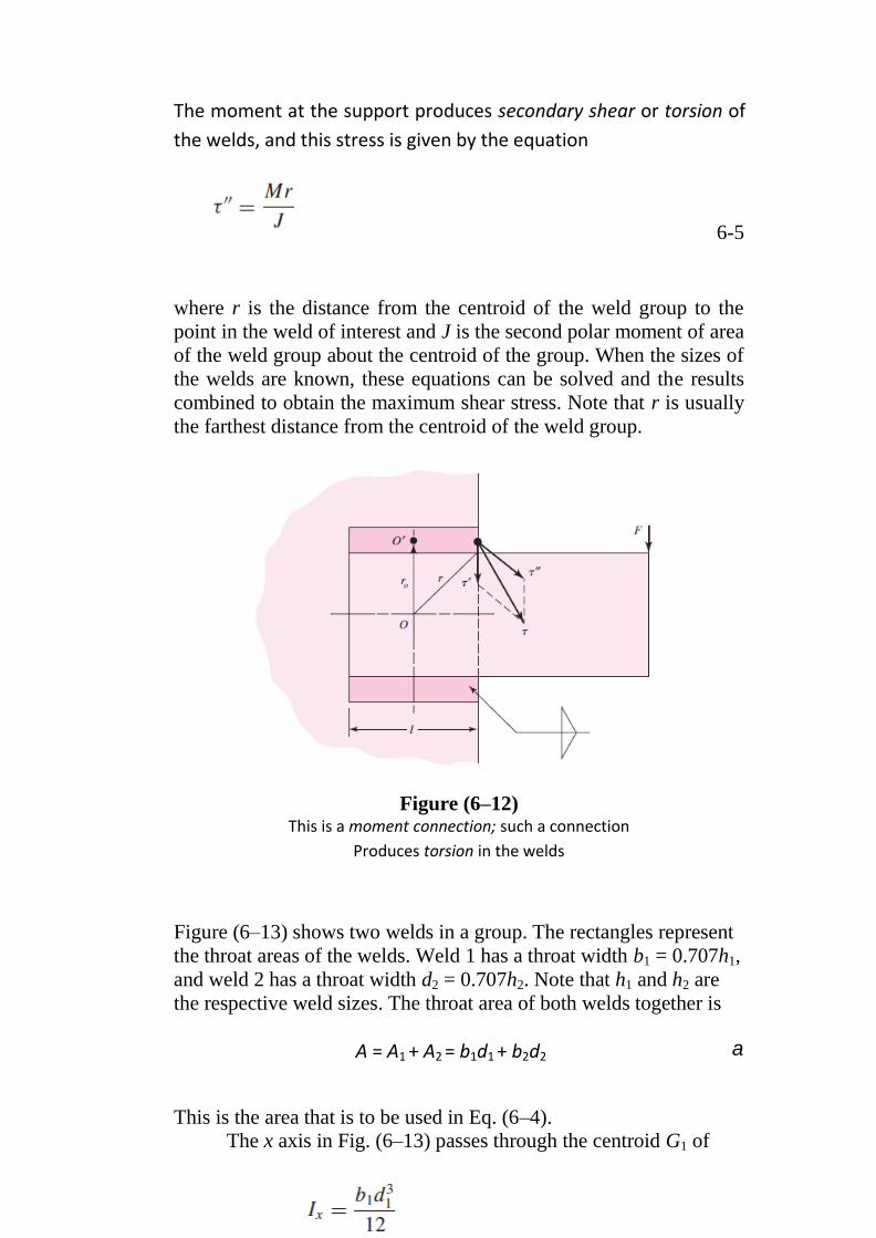
The moment at the support produces secondary shear or torsion of

the welds, and this stress is given by the equation

6-5

where r is the distance from the centroid of the weld group to the

point in the weld of interest and J is the second polar moment of area

of the weld group about the centroid of the group. When the sizes of

the welds are known, these equations can be solved and the results

combined to obtain the maximum shear stress. Note that r is usually

the farthest distance from the centroid of the weld group.

Figure (6–12) This is a moment connection; such a connection

Produces torsion in the welds

Figure (6–13) shows two welds in a group. The rectangles represent

the throat areas of the welds. Weld 1 has a throat width b1 = 0.707h1,

and weld 2 has a throat width d2 = 0.707h2. Note that h1 and h2 are

the respective weld sizes. The throat area of both welds together is

A = A1 + A2 = b1d1 + b2d2 a

This is the area that is to be used in Eq. (6–4).

The x axis in Fig. (6–13) passes through the centroid G1 of

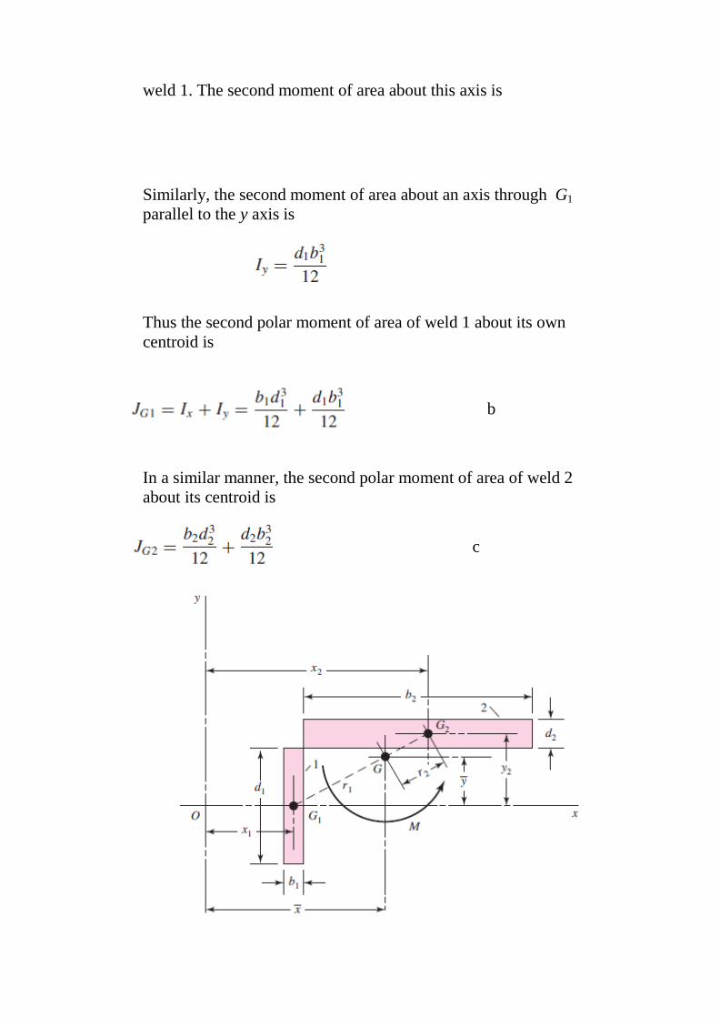
weld 1. The second moment of area about this axis is

Similarly, the second moment of area about an axis through G1

parallel to the y axis is

Thus the second polar moment of area of weld 1 about its own

centroid is

b

In a similar manner, the second polar moment of area of weld 2

about its centroid is

c

Figure (6–13)

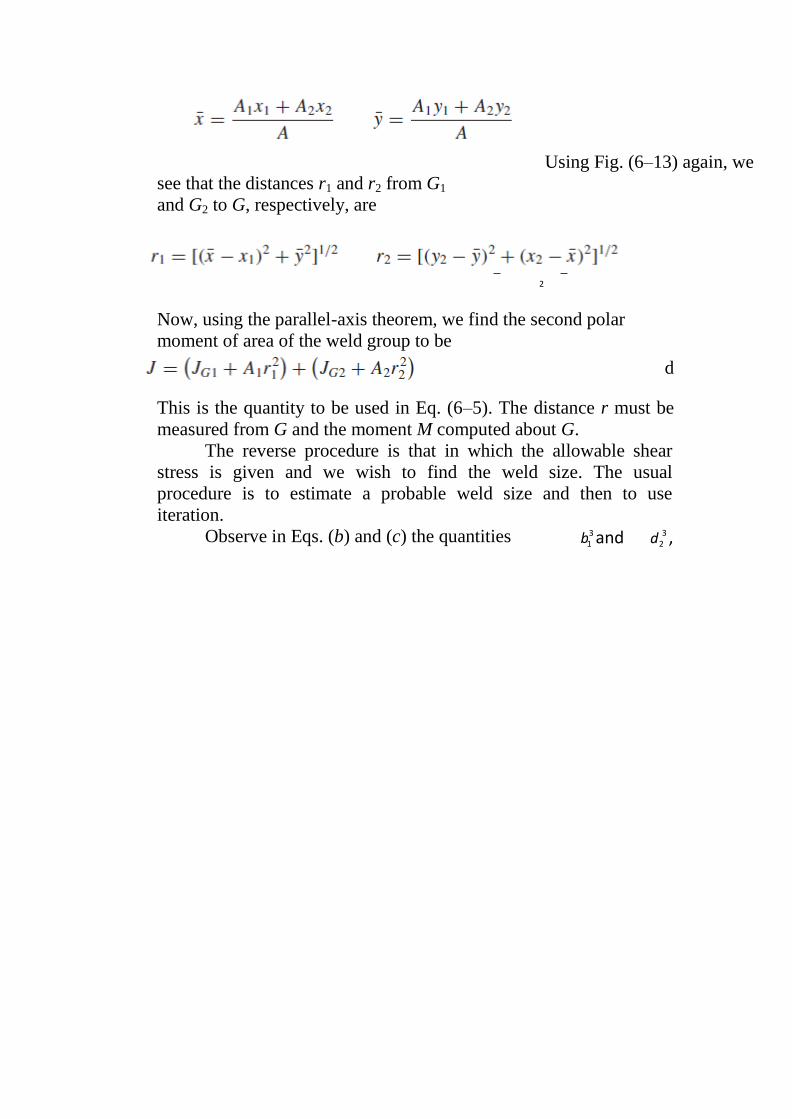
The centroid G of the weld group is located at

2

b 2 1

Using Fig. (6–13) again, we

see that the distances r1 and r2 from G1

and G2 to G, respectively, are

Now, using the parallel-axis theorem, we find the second polar

moment of area of the weld group to be

d

This is the quantity to be used in Eq. (6–5). The distance r must be

measured from G and the moment M computed about G.

The reverse procedure is that in which the allowable shear

stress is given and we wish to find the weld size. The usual

procedure is to estimate a probable weld size and then to use

iteration.

Observe in Eqs. (b) and (c) the quantities 3 and d 3 ,

respectively, which are the cubes of the weld widths. These

quantities are small and can be neglected. This leaves the terms b d 3 /12 and d b3 /12 , which make JG1 and JG2 linear in the weld

1 1 2 2

width. Setting the weld widths b1 and d2 to unity leads to the idea of

treating each fillet weld as a line. The resulting second moment of

area is then a unit second polar moment of area. The advantage of

treating the weld size as a line is that the value of Ju is the same

regardless of the weld size. Since the throat width of a fillet weld is

0.707h, the relationship between J and the unit value is

J = 0.707 h Ju 6-6

in which Ju is found by conventional methods for an area having unit

width. The transfer formula for Ju must be employed when the welds

occur in groups, as in Fig. (6–12). Table (6–1) lists the throat areas

and the unit second polar moments of area for the most common

fillet welds encountered. The example that follows is typical of the

calculations normally made.

EXAMPLE 6–1

A 50-kN load is transferred from a welded fitting into a 200-mm

steel channel as illustrated in Fig. (6–14). Estimate the maximum

stress in the weld.

Figure (6–14) Dimensions in millimeters

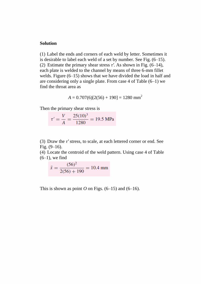
Solution

(1) Label the ends and corners of each weld by letter. Sometimes it

is desirable to label each weld of a set by number. See Fig. (6–15).

(2) Estimate the primary shear stress τ′. As shown in Fig. (6–14),

each plate is welded to the channel by means of three 6-mm fillet

welds. Figure (6–15) shows that we have divided the load in half and

are considering only a single plate. From case 4 of Table (6–1) we

find the throat area as

A = 0.707(6)[2(56) + 190] = 1280 mm2

Then the primary shear stress is

(3) Draw the τ′ stress, to scale, at each lettered corner or end. See

Fig. (9–16).

(4) Locate the centroid of the weld pattern. Using case 4 of Table

(6–1), we find

This is shown as point O on Figs. (6–15) and (6–16).

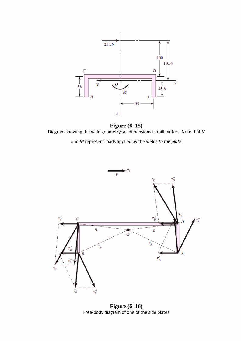
Figure (6–15) Diagram showing the weld geometry; all dimensions in millimeters. Note that V

and M represent loads applied by the welds to the plate

Figure (6–16) Free-body diagram of one of the side plates

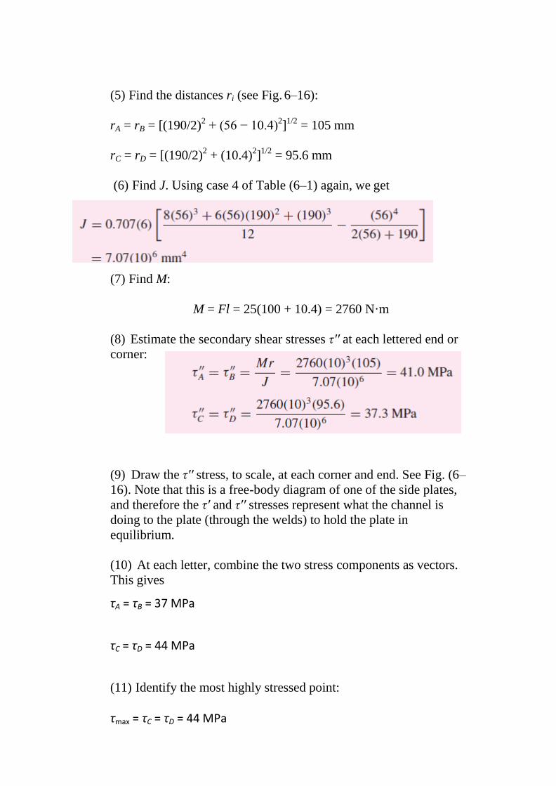
(5) Find the distances ri (see Fig. 6–16):

rA = rB = [(190/2)2 + (56 − 10.4)

2]

1/2 = 105 mm

rC = rD = [(190/2)2 + (10.4)

2]

1/2 = 95.6 mm

(6) Find J. Using case 4 of Table (6–1) again, we get

(7) Find M:

M = Fl = 25(100 + 10.4) = 2760 N·m

(8) Estimate the secondary shear stresses τ′′ at each lettered end or

corner:

(9) Draw the τ′′ stress, to scale, at each corner and end. See Fig. (6–

16). Note that this is a free-body diagram of one of the side plates,

and therefore the τ′ and τ′′ stresses represent what the channel is

doing to the plate (through the welds) to hold the plate in

equilibrium.

(10) At each letter, combine the two stress components as vectors.

This gives

τA = τB = 37 MPa

τC = τD = 44 MPa

(11) Identify the most highly stressed point:

τmax = τC = τD = 44 MPa

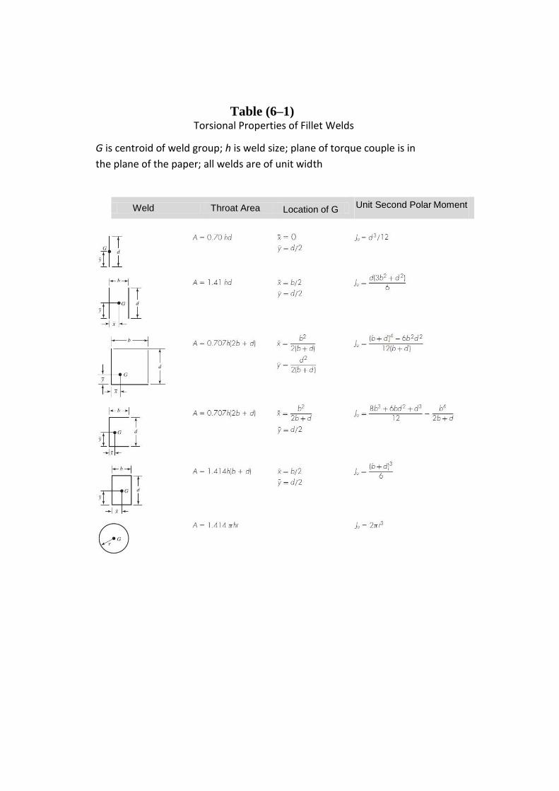
Table (6–1) Torsional Properties of Fillet Welds

G is centroid of weld group; h is weld size; plane of torque couple is in

the plane of the paper; all welds are of unit width

Weld Throat Area Location of G Unit Second Polar Moment

of Area