Sample Chapter 02 Scalar Quantities and Vector Quantities in Mechanics and Motion Analysis
QUANTUM FIELD THEORY IN CONDENSED-MATTER
PHYSICSR. E. S. Otadoy and F. A. Buot
Contents2 INTRODUCTION............................................................................................................................ 23 TIME EVOLUTION OPERATOR (S-MATRIX) FOR A SINGLE PARTICLE................................................3
3.1 BASIC DEFINITION AND PROPERTIES.........................................................................................................33.2 SOLUTION OF THE SCHROEDINGER EQUATION............................................................................................6
4 PICTURES...................................................................................................................................... 94.1 THE SCHROEDINGER PICTURE.................................................................................................................94.2 THE HEISENBERG PICTURE...................................................................................................................104.3 THE INTERACTION PICTURE..................................................................................................................12
5 PROPAGATOR FOR A SINGLE PARTICLE........................................................................................155.1 PROPERTIES OF THE PROPAGATOR.........................................................................................................175.2 PROPAGATOR AND THE GREEN’S FUNCTION............................................................................................195.3 PROPAGATOR AS A TRANSITION AMPLITUDE............................................................................................20
6 IDENTICAL PARTICLES................................................................................................................. 206.1 EXCHANGE DEGENERACY.....................................................................................................................216.2 PERMUTATION OPERATORS..................................................................................................................226.3 PROPERTIES OF P21.............................................................................................................................226.4 THE N-PARTICLE SYSTEM.....................................................................................................................22
7 SECOND QUANTIZATION............................................................................................................. 237.1 CLASSICAL FIELD THEORY.....................................................................................................................23
7.1.1 The Lagrangian as a Functional............................................................................................237.1.2 Variation of a Functional: The Functional Derivative............................................................237.1.3 Hamilton’s Principle (Principle of Least Action) for Fields.....................................................24
7.2 THE HAMILTON FORMALISM................................................................................................................277.2.1 Poisson Bracket of Functionals.............................................................................................297.2.2 An Important Special Case....................................................................................................297.2.3 Time Evolution and Poisson Bracket of Fields.......................................................................29
7.3 CANONICAL QUANTIZATION..................................................................................................................307.3.1 Introduction..........................................................................................................................307.3.2 Quantization Rules for Bosons..............................................................................................337.3.3 Quantization Rules for Fermions..........................................................................................36
8 ZERO-TEMPERATURE GREEN’S FUNCTION...................................................................................388.1.1 Definition of Green’s Function of Many-Body System...........................................................388.1.2 Analytic Properties of the Green’s Function..........................................................................388.1.3 Retarded and Advanced Green’s Function............................................................................38
8.2 QUANTUM CORRELATION FUNCTIONS IN MANY-BODY THEORY..................................................................398.3 PERTURBATION THEORY: FEYNMAN DIAGRAMS........................................................................................39
9 QUANTUM SUPERFIELD THEORY.................................................................................................39
1
9.1 BASIC CONCEPTS IN QUANTUM SUPERFIELD THEORY................................................................................409.1.1 Single-Particle.......................................................................................................................409.1.2 Many-Body System: The Thermal Liouville Space.................................................................42
9.2 QUANTUM DYNAMICS IN LIOUVILLE SPACE.............................................................................................509.2.1 Time Evolution Equations.....................................................................................................509.2.2 The Unitary Superoperator...................................................................................................529.2.3 The Time Evolution Superoperator.......................................................................................539.2.4 The Super-Heisenberg and Super-Interaction Pictures.........................................................549.2.5 Super S-Matrix Theory and Variational Principle in Liouville Space......................................56
9.3 SUPER-GREEN’S FUNCTIONS.................................................................................................................599.4 QUANTUM TRANSPORT EQUATIONS.......................................................................................................639.5 ENERGY BAND DYNAMICS OF BLOCH ELECTRONS.....................................................................................63
9.5.1 Bloch and Wannier Functions...............................................................................................649.5.2 Lattice Weyl-Wigner Formulation of Electron Band Dynamics.............................................679.5.3 Weyl Transformation in Continuous Phase Space.................................................................779.5.4 Integral Form of the Weyl Transform of the Commutator and Anticommutator..................90
BIBLIOGRAPHY.................................................................................................................................. 9110 REFERENCES........................................................................................................................... 94
1 Introduction101Equation Chapter 1 Section 0
See Chapter 1 of McMahon (McMahon, 2008) (introductory comments on quantum field theory as a theoretical framework combining quantum mechanics and the special theory of relativity):
Quantum field theory is a theoretical framework that combines quantum mechanics and Einstein’s special theory of relatativity (McMahon, 2008). The key ideas in quantum theory are the operators representing measurable quantities known also as observables, the uncertainty principle, and the commutation relations of operators. Measurable quantities in classical mechanics become operators in quantum mechanics. The transition from measurable quantities to operators is called quantization. For instance, the energy equation
2102\* MERGEFORMAT (..)becomes the Schroedinger’s equation in
3103\* MERGEFORMAT(..)in quantum mechanics where, the following transformations are used:
2

In the special theory of relativity, the mass-energy relation 4104\* MERGEFORMAT (..)
and its variant 5105\* MERGEFORMAT (..)
implies conversion of mass to energy and vice versa, that is, matter can now be created or destroyed. The number of particles therefore is no longer fixed.The first attempt to construct a relativistic quantum equation based on Eq. 105, which results to
6106\* MERGEFORMAT (..)Continue reading page 3 of McMahon (McMahon, 2008).
2 Time Evolution Operator (S-Matrix) for a Single Particle712Equation Chapter 2 Section 1
2.1 Basic Definition and Properties
The nature of time is one of the greatest ironies in physics. In classical mechanics, time is considered as a parameter whereas in the special theory of relativity, time has been elevated as a dynamical variable. In quantum mechanics, time is still considered as a parameter, so it makes no sense to talk about its eigenvalues and eigenstates. With its elevation as a dynamical variable in the special theory of relativity, it is expected that in quantum field theory time would emerge as an observable. However, the concept of time operator is still untenable even in quantum field theory.
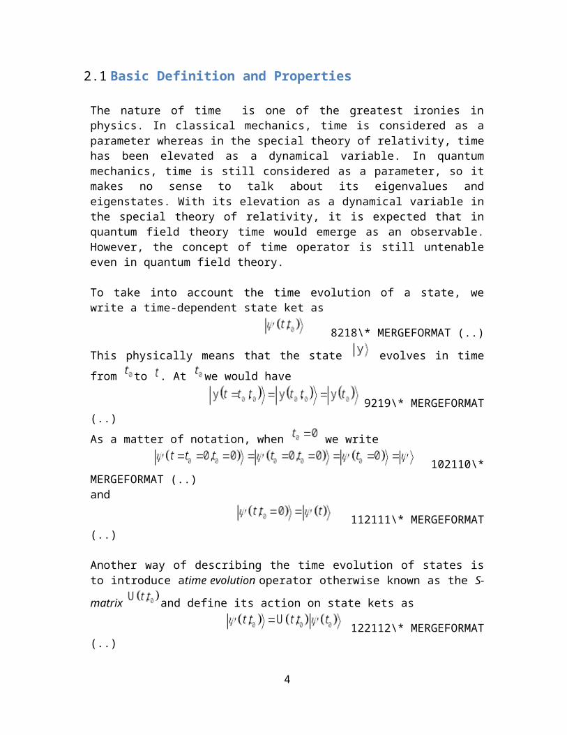
To take into account the time evolution of a state, we write a time-dependent state ket as
8218\* MERGEFORMAT (..)This physically means that the state evolves in time from to . At we would have
3
9219\*MERGEFORMAT (..)As a matter of notation, when we write
102110\*MERGEFORMAT (..)and
112111\* MERGEFORMAT(..)
Another way of describing the time evolution of states is to introduce atime evolution operator otherwise known as the S-matrix and define its action on state kets as
122112\*MERGEFORMAT (..)The properties of this operator can be obtained from physical considerations:
1. Unitarity
Recall that in order for the probabilistic interpretation of quantum mechanics to hold ground, we require that states kets are normalized, that is,
132113\* MERGEFORMAT (..)For quantum theory to be consistent we should require this to hold true regardless of time,
142114\*MERGEFORMAT (..)Since the corresponding bra of Eq. 2112 is
152115\*MERGEFORMAT (..)Eq. 2114 implies that,
162116\* MERGEFORMAT(..)where is the identity operator. Eq. 2116 can only be true if
4
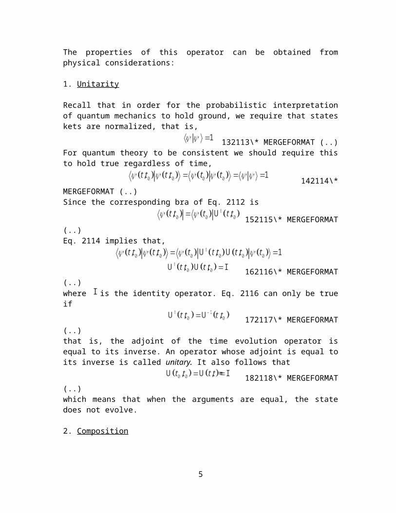
172117\* MERGEFORMAT(..)that is, the adjoint of the time evolution operator is equal to its inverse. An operator whose adjoint is equal to its inverse is called unitary. It also follows that
182118\* MERGEFORMAT(..)which means that when the arguments are equal, the state does not evolve.
2. Composition
The composition property stems from the evolution of the state from to then from to . This can be accomplished by successive
application of the time evolution operator as follows,
192119\* MERGEFORMAT(..)The evolution of the state from to then from to is equivalent to its evolution from to represented by Eq. 2112. Thus one can have
202120\*MERGEFORMAT (..)and therefore,
212121\* MERGEFORMAT(..)It follows that when we slice time N times
222122\*MERGEFORMAT (..)Eqs. 2121 and 2122 are called composition property.
It is to be noted also that from Eq. 2118 and from the composition property,
which shows that, 232123\*
MERGEFORMAT (..)
3. Time Evolution
5
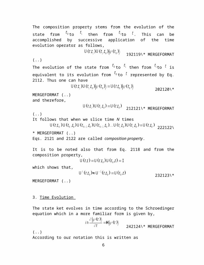
The state ket evolves in time according to the Schroedinger equation which in a more familiar form is given by,
242124\* MERGEFORMAT(..)According to our notation this is written as
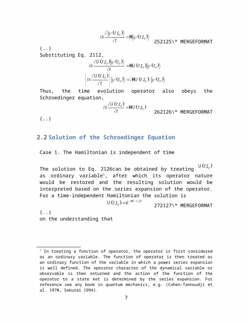
252125\* MERGEFORMAT(..)Substituting Eq. 2112,
Thus, the time evolution operator also obeys the Schroedinger equation,
262126\* MERGEFORMAT(..)
2.2 Solution of the Schroedinger Equation
Case 1. The Hamiltonian is independent of time
The solution to Eq. 2126can be obtained by treating as ordinary variable1, after which its operator nature would be restored and the resulting solution would be interpreted based on the series expansion of the operator. For a time-independent Hamiltonian the solution is
272127\* MERGEFORMAT(..)on the understanding that
1 In treating a function of operator, the operator is first considered as an ordinary variable. The function of operator is then treated as an ordinary function of the variable in which a power series expansion is well defined. The operator character of the dynamical variable or observable is then returned and the action of the function of the operator to a state ket is determined by the series expansion. For reference see any book in quantum mechanics, e.g. (Cohen-Tannoudji et al. 1970, Sakurai 1994).
6
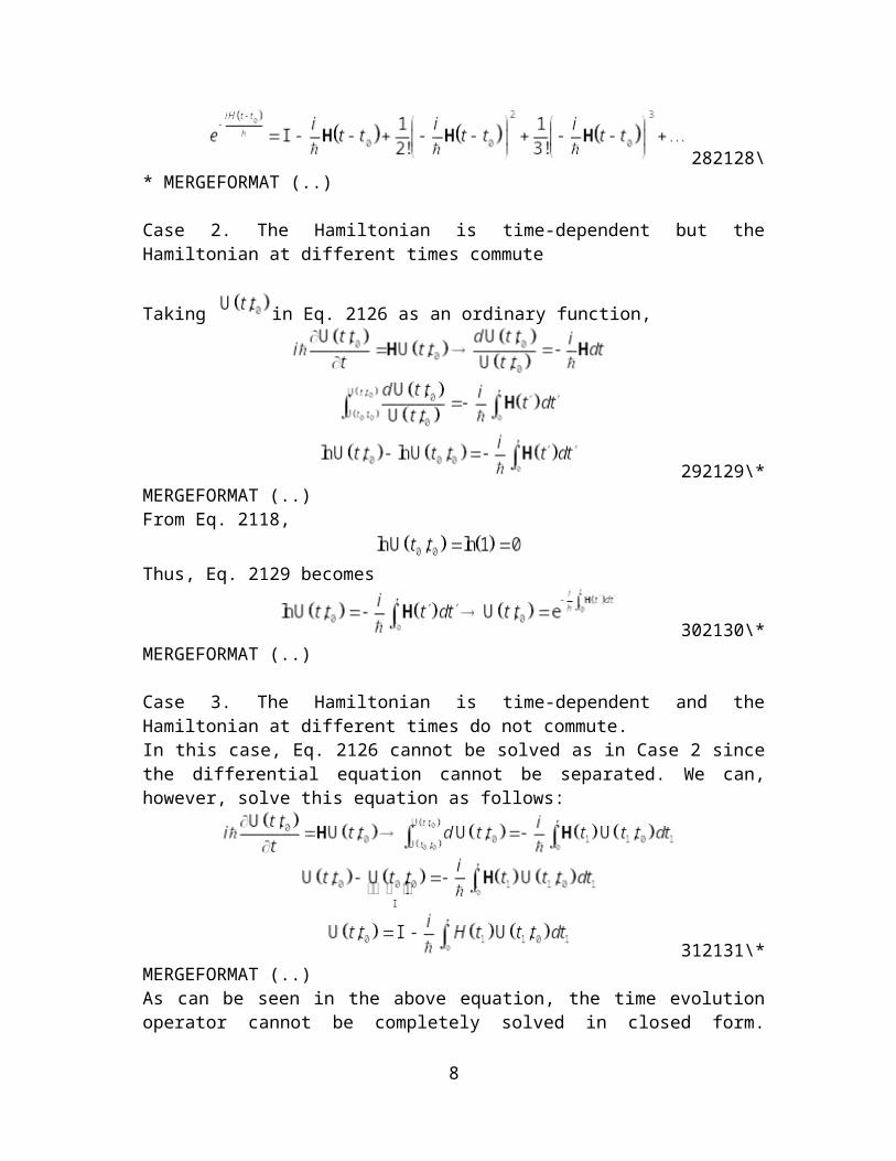
282128\* MERGEFORMAT (..)
Case 2. The Hamiltonian is time-dependent but the Hamiltonian at different times commute
Taking in Eq. 2126 as an ordinary function,
292129\*MERGEFORMAT (..)From Eq. 2118,
Thus, Eq. 2129 becomes
302130\*MERGEFORMAT (..)
Case 3. The Hamiltonian is time-dependent and the Hamiltonian at different times do not commute.In this case, Eq. 2126 cannot be solved as in Case 2 since the differential equation cannot be separated. We can, however, solve this equation as follows:
312131\*MERGEFORMAT (..)As can be seen in the above equation, the time evolution operator cannot be completely solved in closed form. However, we can arrive at an approximate solution by iteration. Following Eq. 2131, can be written as
7
322132\*MERGEFORMAT (..)Substituting Eq. 2132 to Eq. 2131 one obtains,
332133\* MERGEFORMAT (..)One may note that appears in the second integral of Eq. 2133. An expression for this can be derived by the replacement and
in Eq.2132. When the resulting expression is substituted to Eq. 2133, one obtains
Simplifying
342134\*MERGEFORMAT (..)If the process is iterated, we arrive at the so-called Dyson series,
352135\* MERGEFORMAT (..)At this juncture it is convenient to introduce the time-ordering operator useful in dealing with product of operators that do not commute at different times like the integrand in Eq.2135. It is just an instruction to arrange the product so that the right-most operator corresponds to the earliest time. For instance, if ,
To include different possibilities, we introduce the Heaviside unit-step function defined by
8
362136\* MERGEFORMAT(..)and that
372137\*MERGEFORMAT (..)The action of is then expressed as
382138\*MERGEFORMAT (..)The step functions assure that the two possibilities do not occur at the
same time. Now consider the integral :
Interchanging the indices 1 and 2 in the second integral shows that the two integrals are actually the same. Thus,
392139\*MERGEFORMAT (..)If we follow the same steps, one can write Eq.2135 as
402140\* MERGEFORMAT (..)This can further be written symbolically as
412141\*MERGEFORMAT (..)
3 Pictures4222Equation Chapter 2 Section 2The expectation value of an operator (average value of a dynamical variable) is given by
9
432243\* MERGEFORMAT (..)The time-dependent expectation value can also be written as
442244\*MERGEFORMAT (..)As can be seen in Eq. 2244, one can take note two schemes of describing the dynamics of the expectation value:
Scheme 1
452245\*MERGEFORMAT (..)
Scheme 2
462246\*MERGEFORMAT (..)
3.1 The Schroedinger PictureScheme 1 is the more famaliar picture of quantum mechanics in which state kets are time-dependentwhile operators associated with dynamical variables are time-independent,
472247\*MERGEFORMAT (..)It is actually the picture we are actually following so far. It is called the Schroedinger picture. It is also well known that even though state kets are time-dependent, eigenkets (which constitute a basis) remain time-independent,
482248\* MERGEFORMAT (..)If the state ket is initially given by
it evolves as
492249\*MERGEFORMAT (..)For time-independent Hamiltonian and if is its eigenket, we have
10
502250\*MERGEFORMAT (..)Thus, the time evolution operator introduces a phase change of the coefficients.
3.2 The Heisenberg PictureThe Heisenberg picture adopts Scheme 2 of describing quantum dynamics in which state kets are time-independent and operators are time-dependent, according to Eq.2246,
512251\*MERGEFORMAT (..)where the subscript H indicates that the operator is in the Heisenberg picture while the subscript S indicates that the operator is in the Schroedinger picture. To simplify things, we take and assume that the Hamiltonian is time-independent. Thus one can have,
522252\* MERGEFORMAT(..)Let us give a special designation to Eq. 2252,
532253\* MERGEFORMAT(..)In this notation, Eqs.2247 and2251 become, respectively,
542254\*MERGEFORMAT (..)which describes the time evolution of Schroedinger picture state ket and
552255\*MERGEFORMAT (..)which describes the time evolution of Heisenberg picture operator.
At the Heisenberg and the Schroedinger pictures coincide,
562256\* MERGEFORMAT(..)
572257\* MERGEFORMAT (..)such that Eq. 2255 can also be written as
11
582258\*MERGEFORMAT (..)
In general, for , the Schroedinger and the Heisenberg pictures coincide,
592259\* MERGEFORMAT (..)602260\*
MERGEFORMAT (..)and that Eq.2251 can also be written as
612261\*MERGEFORMAT (..)
The Heisenberg Equation of MotionThe Heisenberg-picture operators evolve in time according to the equation,
622262\*MERGEFORMAT (..)This is called the Heisenberg equation of motion.
PROOF OF HEISENBERG EQUATION OF MOTION
Let us use Eq. 2251 in evaluating the derivative of Heisenberg-picture operators:
632263\*MERGEFORMAT (..)
From Eq. 2126
642264\* MERGEFORMAT(..)
652265\*MERGEFORMAT (..)Substituting to Eq.2263
12
662266\*MERGEFORMAT (..)
Base Kets in the Heisenberg PictureThe eigenvalue equation for the Schroedinger-picture observable is given by Eq. 2248 and it can be considered as a Heisenberg-picture observable at ,
672267\* MERGEFORMAT(..)For finite time ,
682268\*MERGEFORMAT (..)Whereas the state ket is time-independent in the Heisenberg picture, the basis kets change with time as
692269\* MERGEFORMAT(..)In general, one can have the result for the basis kets
702270\*MERGEFORMAT (..)Transition AmplitudesAnother quantity which is important in our future studies of many-particle system is the transition amplitude, which is the probability amplitude2 for a particle initially prepared in the state to be
2 The probability is the square of the probability amplitude.
13
found in the eigenstate of observable . It is given in the Schroedinger picture by
712271\*MERGEFORMAT (..)For
722272\*MERGEFORMAT (..)In the Heisenberg picture,
732273\*MERGEFORMAT (..)Thus, the expressions for the transitition amplitude are the same in both Schroedinger and Heisenberg pictures.If is an eigenstate of ,
742274\*MERGEFORMAT (..)
3.3 The Interaction PictureThe interaction picture is most useful when the Hamiltonian can be split into,
752275\* MERGEFORMAT (..)where is the Hamiltonian whose eigenkets and eigenvalues are already known while W is the remaining part of the total Hamiltonian whose eigenkets and eigenvalues are unknown. The state ket in the interaction picture is defined by
762276\*MERGEFORMAT (..)The subscript I indicates that the quantity is in the interaction picture. Obviously, at the two pictures coincide. For operators representing observables, transformation from the Schroedinger picture to interaction picture is defined by
772277\* MERGEFORMAT(..)The unknown part of the total Hamiltonian can therefore be written in the interaction picture as
782278\* MERGEFORMAT(..)The evolution of the state ket is given by
14
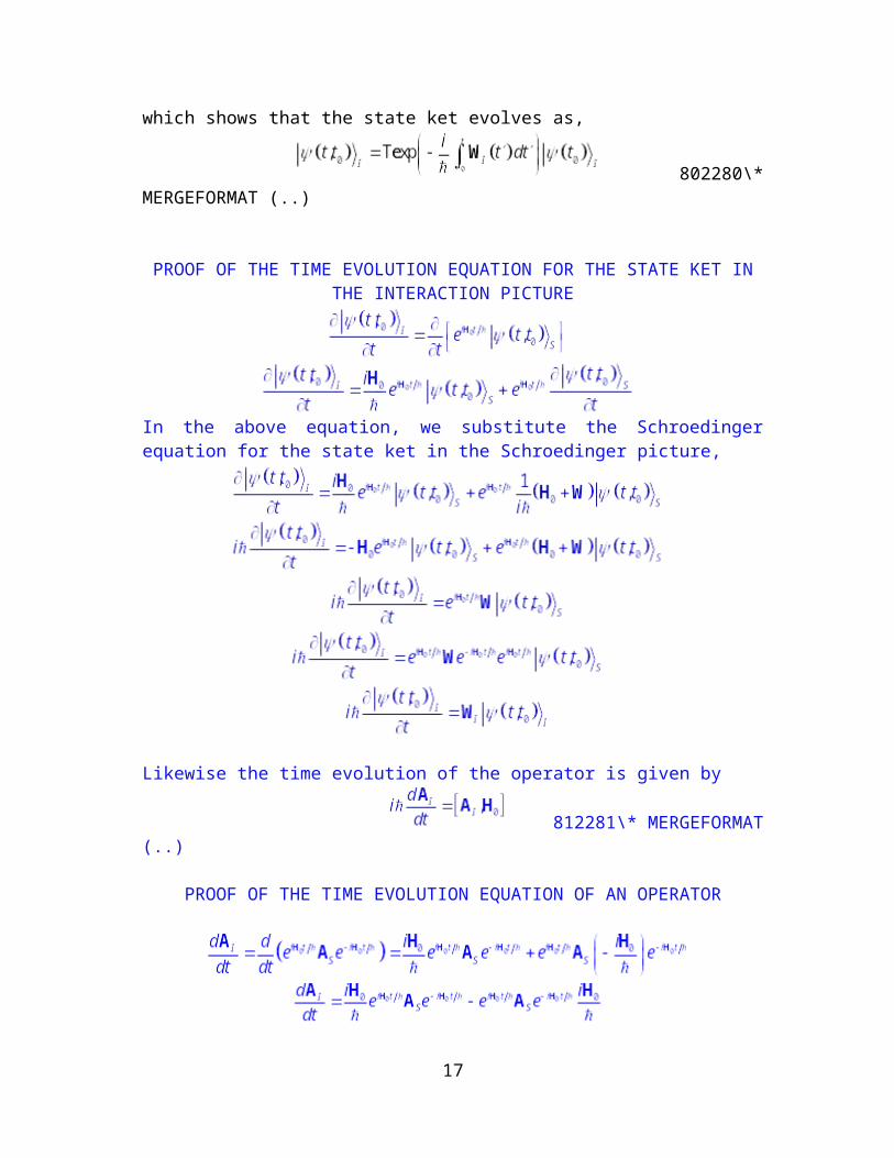
792279\*MERGEFORMAT (..)which shows that the state ket evolves as,
802280\*MERGEFORMAT (..)
PROOF OF THE TIME EVOLUTION EQUATION FOR THE STATE KET IN THE INTERACTION PICTURE
In the above equation, we substitute the Schroedinger equation for the state ket in the Schroedinger picture,
Likewise the time evolution of the operator is given by
812281\* MERGEFORMAT (..)
PROOF OF THE TIME EVOLUTION EQUATION OF AN OPERATOR
15
which is Eq.2281.
One can see that in this picture, both the state ket and the operator are time-dependent contrary to the Schroedinger and Heisenberg pictures.
The real value of the interaction picture lies in its use of its corresponding time-evolution operator. We define it as
822282\*MERGEFORMAT (..)and from Eq.2279 it satisfies the equation
832283\* MERGEFORMAT(..)Following the same steps as in the derivation of Eq.2135, the solution of Eq.2283 can be written as
842284\* MERGEFORMAT (..)
852285\* MERGEFORMAT (..)
Let us explore the connection between the time evolution operator in the Schroedinger picture to that of the interaction picture. To this end we can make use of Eq.2276
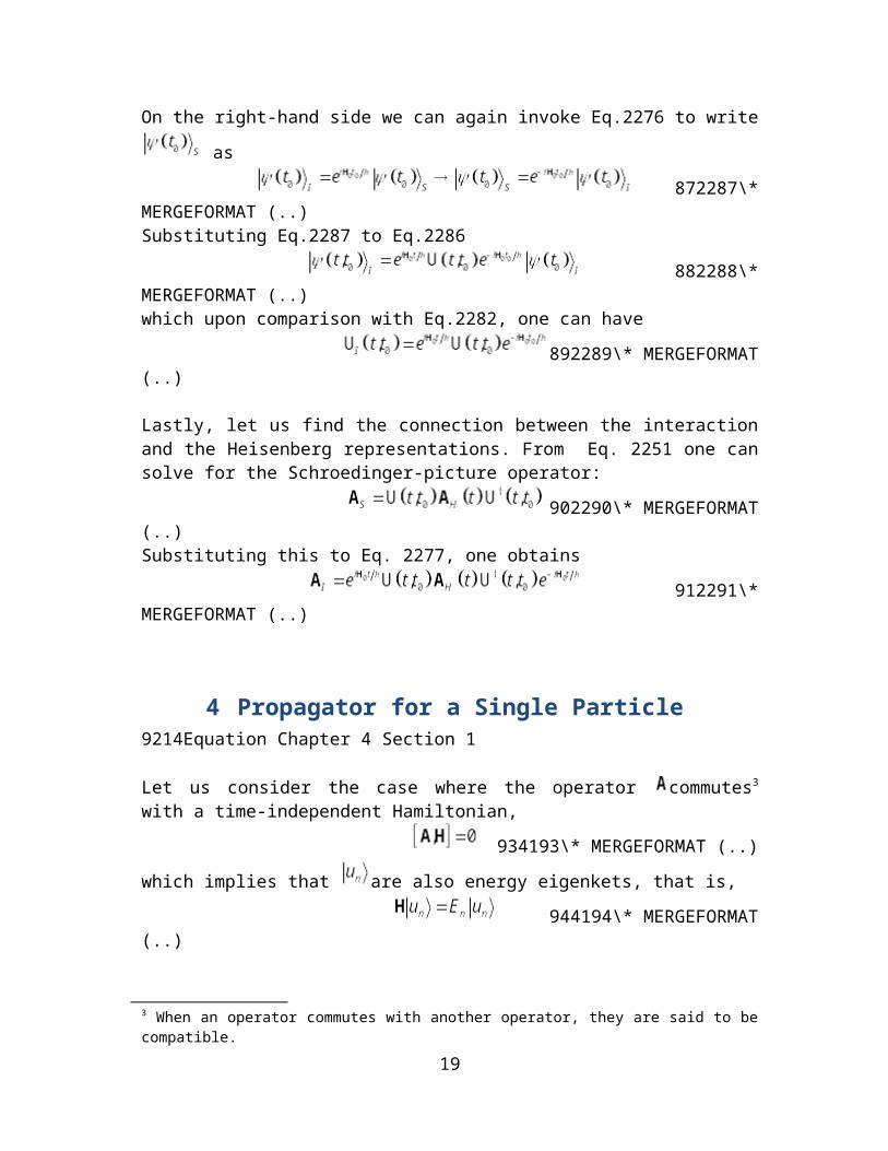
862286\*MERGEFORMAT (..)On the right-hand side we can again invoke Eq.2276 to write as
16
872287\*MERGEFORMAT (..)Substituting Eq.2287 to Eq.2286
882288\*MERGEFORMAT (..)which upon comparison with Eq.2282, one can have
892289\*MERGEFORMAT (..)
Lastly, let us find the connection between the interaction and the Heisenberg representations. From Eq. 2251 one can solve for the Schroedinger-picture operator:
902290\*MERGEFORMAT (..)Substituting this to Eq. 2277, one obtains
912291\*MERGEFORMAT (..)
4 Propagator for a Single Particle9214Equation Chapter 4 Section 1
Let us consider the case where the operator commutes3 with a time-independent Hamiltonian,
934193\* MERGEFORMAT (..)which implies that are also energy eigenkets, that is,
944194\* MERGEFORMAT (..)
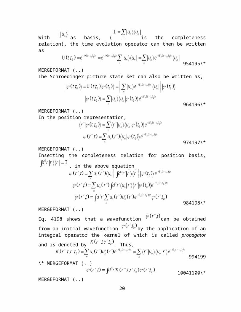
With as basis, ( is the completeness relation), the time evolution operator can then be written as
954195\*MERGEFORMAT (..)The Schroedinger picture state ket can also be written as,
3 When an operator commutes with another operator, they are said to be compatible.
17

964196\*MERGEFORMAT (..)In the position representation,
974197\*MERGEFORMAT (..)
Inserting the completeness relation for position basis, , in the above equation
984198\*MERGEFORMAT (..)Eq. 4198 shows that a wavefunction can be obtained from an initial wavefunction by the application of an integral operator the kernel of which is called propagator and is denoted by . Thus,
994199\* MERGEFORMAT (..)
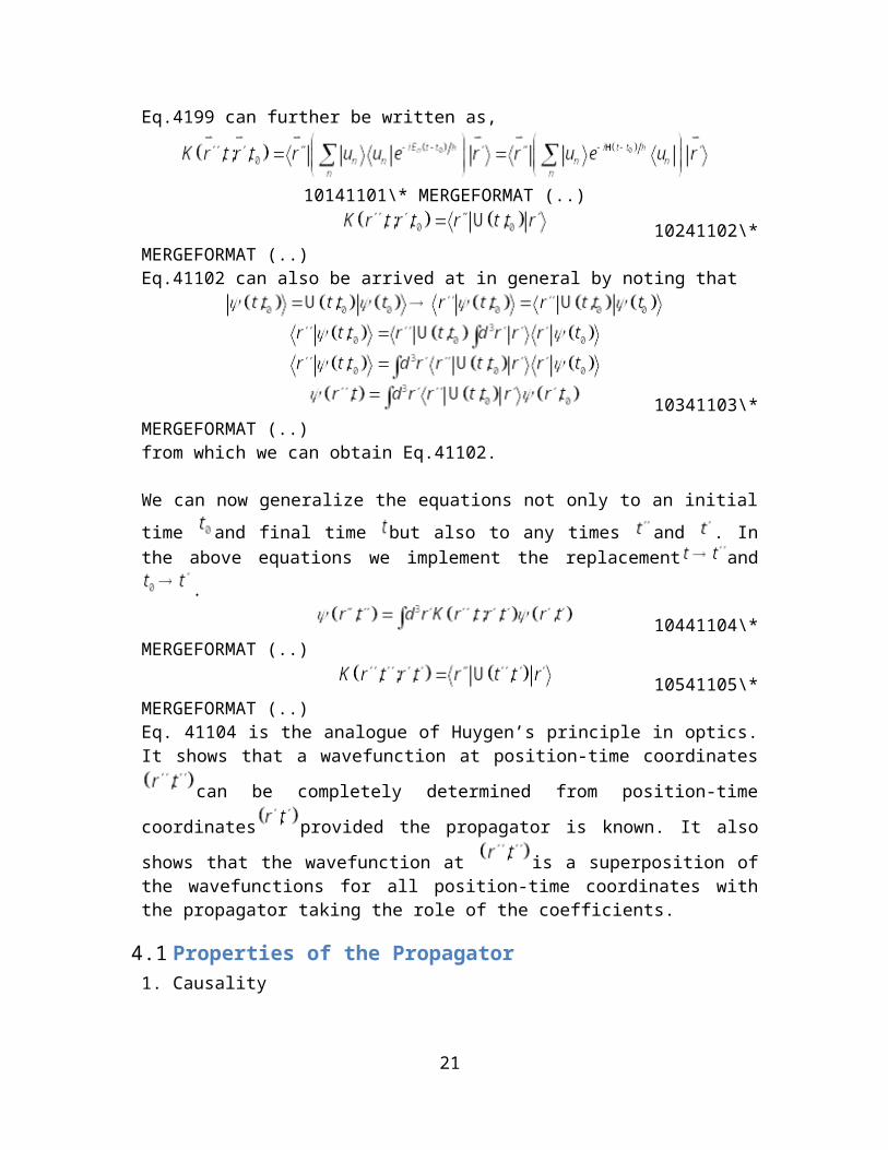
10041100\*MERGEFORMAT (..)Eq.4199 can further be written as,
10141101\* MERGEFORMAT (..)10241102\*
MERGEFORMAT (..)Eq.41102 can also be arrived at in general by noting that
18
10341103\*MERGEFORMAT (..)from which we can obtain Eq.41102.
We can now generalize the equations not only to an initial time and final time but also to any times and . In the above equations we implement the replacement and .
10441104\*MERGEFORMAT (..)
10541105\*MERGEFORMAT (..)Eq. 41104 is the analogue of Huygen’s principle in optics. It shows that a wavefunction at position-time coordinates can be completely determined from position-time coordinates provided the propagator is known. It also shows that the wavefunction at
is a superposition of the wavefunctions for all position-time coordinates with the propagator taking the role of the coefficients.
4.1 Properties of the Propagator1. Causality
To take into account causlity (the cause precedes the effect) we require that
10641106\*MERGEFORMAT (..)
2. CompositionThe composition property for the propagator is expressed as
10741107\*MERGEFORMAT (..)
PROOF OF COMPOSITION PROPERTY
19
This follows from the composition property of the time-evolution operator 2121
Using the completeness relation for the position basis,
which is Eq.41107. The composition property can also be derived by iterating Eq.41104 by writing
10841108\*MERGEFORMAT (..)and substituting back to Eq. 41104,
10941109\*MERGEFORMAT (..)which is the same as Eq.41107.
3. Another property of the propagator can be obtained by noting that when in Eq.41105,
11041110\*MERGEFORMAT (..)4. For , the propagator obeys the Schroedinger equation,
11141111\* MERGEFORMAT (..)
PROOF OF THE SCHROEDINGER EQUATION FOR THE PROPAGATOR
The proof follows from the Schroedinger equation for the time-evolution operator, Eq.2126,
20
which is Eq.41111.
4.2 Propagator and the Green’s FunctionThe requirement for causality expressed by Eq.41106 can be collectively written as
11241112\*MERGEFORMAT (..)where is the Heaviside unit-step function defined by
11341113\*MERGEFORMAT (..)It is to be noted that
11441114\*MERGEFORMAT (..)The causality requirement, together with Property 3, enables us to write the Schroedinger’s equation for the propagator as
11541115\* MERGEFORMAT (..)
21
Thus, apart from the factor , the propagator is the Green’s function of the Schroedinger equation for the wavefunction and provides another mathematical justification for Eq.411044.
4.3 Propagator as a Transition AmplitudeLet us go back to Eq.4199
If we consider the position eigenkets as the basis, we have11641116\* MERGEFORMAT
(..)and
11741117\*MERGEFORMAT (..)and thus,
11841118\*MERGEFORMAT (..)In this form, the propagator can be interpreted as the probability amplitude in going from one position-time coordinates to another position-time coordinates.
The result 41118 can actually be directly obtained from Eq.41105,
11941119\*MERGEFORMAT (..)
5 Identical ParticlesIn the previous sections we were dealing with a single particle which is not the domain of many-body physics and is a clear overkill with
4 Recall that the Green’s function of a differential equation is given by
and its solution is .
22

more difficult concepts of S-matrix and propagators. We could have used the quantum mechanics we know in an elementary quantum mechanics course and not bother about these concepts. The previous sections however lay the foundation as the same concepts will be used in developing a many-body theory, which we start in this section by studying a system composed of the same species5 of particles known as identical particles.In classical mechanics, identical particles are distinguishable in the sense that we can assign a trajectory to each particle. Since the concept of trajectory breaks down in quantum mechanics, there is no way that we can label the individual particles. In this sense, identical quantum particles are indistinguishable.
5.1 Exchange Degeneracy12015Equation Chapter 5 Section 1Let us first consider a system of three nonidentical particles. With each of the three particles taken separately we can associate a state space and observables acting in that space. If we number the particles 1,2, and 3 the state spaces are respectively,
. The state spaces of the three-particle system is given by the tensor product,
12151121\*MERGEFORMAT (..)Now consider an observable defined in state space . If we consider the three particles as identical, then correspondingly there are observables and in state spaces and respectively (identical particles have the same intrinsic properties). Furthermore, these particles have the same set of eigenvalues. If the
basis in the state spaces are respectively, ,
, and , the basis in the state space is
12251122\*MERGEFORMAT (..)where are the associated individual or collective quantum numbers. The vectors are the eigenvectors of the extension of , and in the state space with the
5 The particles have the same properties.
23
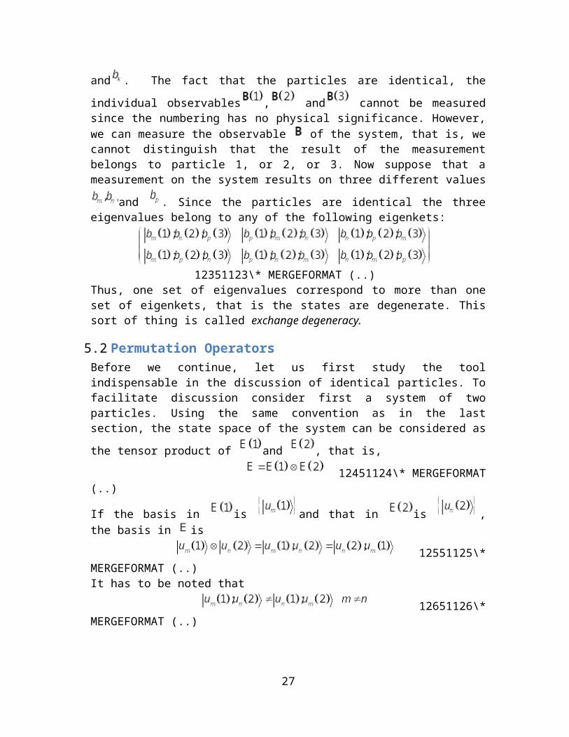
respective eigenvalues , , and . The fact that the particles are identical, the individual observables , and cannot be measured since the numbering has no physical significance. However, we can measure the observable of the system, that is, we cannot distinguish that the result of the measurement belongs to particle 1, or 2, or 3. Now suppose that a measurement on the system results on three different values and . Since the particles are identical the three eigenvalues belong to any of the following eigenkets:
12351123\* MERGEFORMAT (..)Thus, one set of eigenvalues correspond to more than one set of eigenkets, that is the states are degenerate. This sort of thing is called exchange degeneracy.
5.2 Permutation OperatorsBefore we continue, let us first study the tool indispensable in the discussion of identical particles. To facilitate discussion consider first a system of two particles. Using the same convention as in the last section, the state space of the system can be considered as the tensor product of and , that is,
12451124\* MERGEFORMAT(..)
If the basis in is and that in is , the basis in is
12551125\*MERGEFORMAT (..)It has to be noted that
12651126\*MERGEFORMAT (..)The exchange of labels can be effected by the permutation operator
defined as a linear operator whose action on the basis ket is:12751127\*
MERGEFORMAT (..)Its action on an arbitrary ket in the state space can be obtained by expanding the ket in the basis 51125.
24
5.3 Properties of P21
1. is the inverse of itself
PROOF
This section is taken from my lecture notes on Identical Particles. To continue, read my lecture notes.
5.4 The N-Particle SystemSee Section 1.1 of Balisot and Ripka (Balizot & Ripka). Also see Coleman (Coleman, 2013).
6 Second Quantization
6.1 Classical Field Theory12816Equation Chapter 6 Section 1
6.1.1 The Lagrangian as a Functional
See Page 32 of Greiner et al. (Greiner & Reinhardt, 1996).
In particle mechanics the Lagrangian is a function of the generalized
coordinates and generalized velocity . In field theory, the
Lagrangian is a function of the field and its time derivative
. A field is a function of the coordinates. So, the Lagrangian is a function of a function. In short, it is a mapping or correspondence between a function and real numbers (in general a complex number), a quantity called functional. We can think of a functional as a machine whose input is a function and whose output is a real number.
More formally, a functional is a mapping of a normed linear space of functions (this linear space of functions is a Banach space6) to the 6 A Banach space is a linear vector space endowed with a norm [see Section 1.2 of Tarasov (Tarasov, 2008)].
25
field7 of real or complex numbers. This statement can written symbolically as
12961129\* MERGEFORMAT(..)
where , that is the linear space of functions.
The Lagrangian in field theory belongs to this class of quantities, that is, the Lagrangian in field theory is a functional,
13061130\*MERGEFORMAT (..)The functional depends on the values of the field and its time derivative at each point in space with the coordinates acting as continuous index. It does not depend explicitly on the coordinates.
6.1.2 Variation of a Functional: The Functional DerivativeSee Section 2.3 of Greiner et al. (Greiner & Reinhardt, 1996).
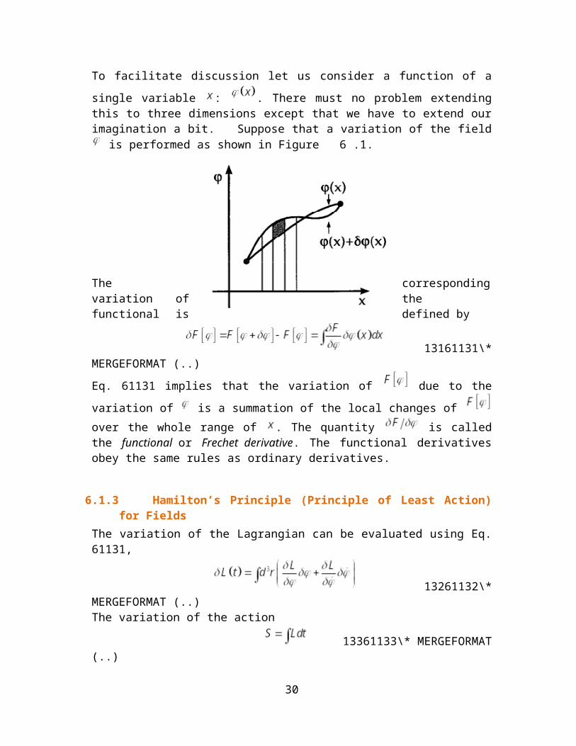
To facilitate discussion let us consider a function of a single variable : . There must no problem extending this to three dimensions except that we have to extend our imagination a bit. Suppose that a variation of the field is performed as shown in Figure 6.1.
The corresponding variation of the functional is defined by
13161131\* MERGEFORMAT (..)
7 Field in this context is different from the field You can think of field here as a set. Thus a field of complex numbers simply means a set of complex numbers.
26
Figure 6.1 Variation of the field [taken from (Greiner& Reinhardt, 1996)].
Eq. 61131 implies that the variation of due to the variation of is a summation of the local changes of over the whole range of
. The quantity is called the functional or Frechet derivative. The functional derivatives obey the same rules as ordinary derivatives.
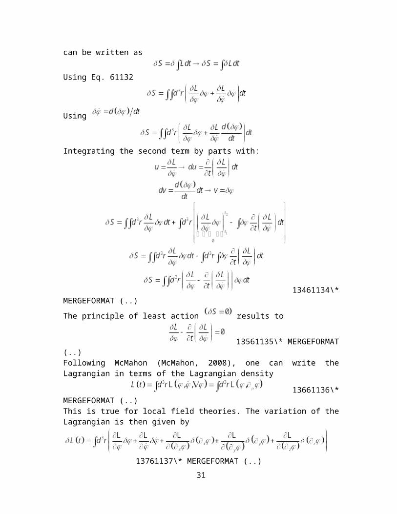
6.1.3 Hamilton’s Principle (Principle of Least Action) for FieldsThe variation of the Lagrangian can be evaluated using Eq. 61131,
13261132\*MERGEFORMAT (..)The variation of the action
13361133\* MERGEFORMAT (..)can be written as
Using Eq. 61132
Using
Integrating the second term by parts with:
13461134\*MERGEFORMAT (..)
27
The principle of least action results to
13561135\* MERGEFORMAT(..)Following McMahon (McMahon, 2008), one can write the Lagrangian in terms of the Lagrangian density
13661136\*MERGEFORMAT (..)This is true for local field theories. The variation of the Lagrangian is then given by
13761137\* MERGEFORMAT (..)
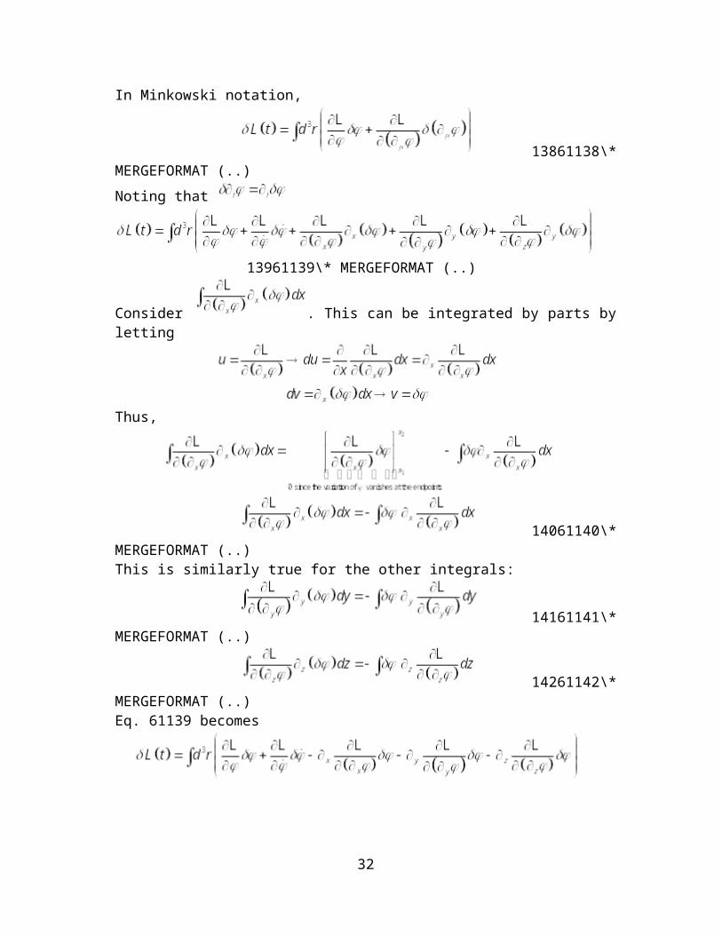
In Minkowski notation,
13861138\*MERGEFORMAT (..)Noting that
13961139\* MERGEFORMAT (..)
Consider . This can be integrated by parts by letting
Thus,
14061140\*MERGEFORMAT (..)This is similarly true for the other integrals:
28
14161141\*MERGEFORMAT (..)
14261142\*MERGEFORMAT (..)Eq. 61139 becomes
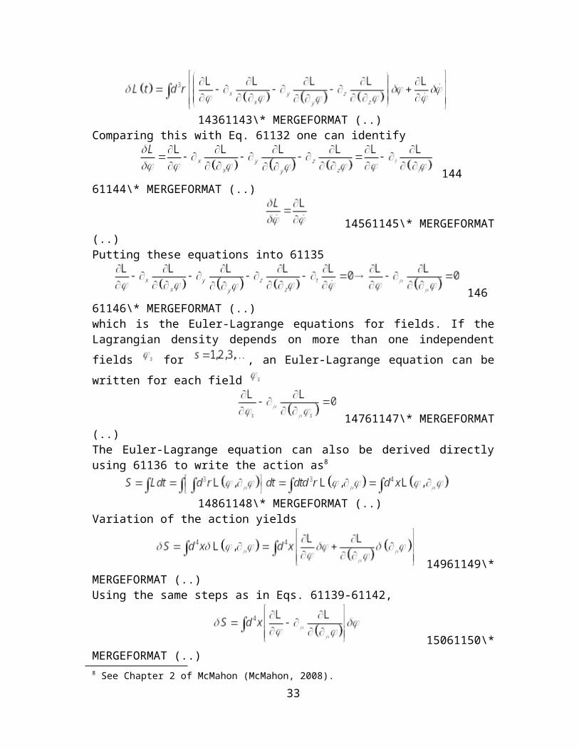
14361143\* MERGEFORMAT (..)
Comparing this with Eq. 61132 one can identify
14461144\* MERGEFORMAT (..)
14561145\* MERGEFORMAT (..)Putting these equations into 61135
14661146\* MERGEFORMAT (..)which is the Euler-Lagrange equations for fields. If the Lagrangian density depends on more than one independent fields for
, an Euler-Lagrange equation can be written for each field
14761147\*MERGEFORMAT (..)The Euler-Lagrange equation can also be derived directly using 61136 to write the action as8
14861148\* MERGEFORMAT (..)
Variation of the action yields
8 See Chapter 2 of McMahon (McMahon, 2008).
29
14961149\*MERGEFORMAT (..)Using the same steps as in Eqs. 61139-61142,
15061150\*MERGEFORMAT (..)The principle of least action then results to Eq. 61146.
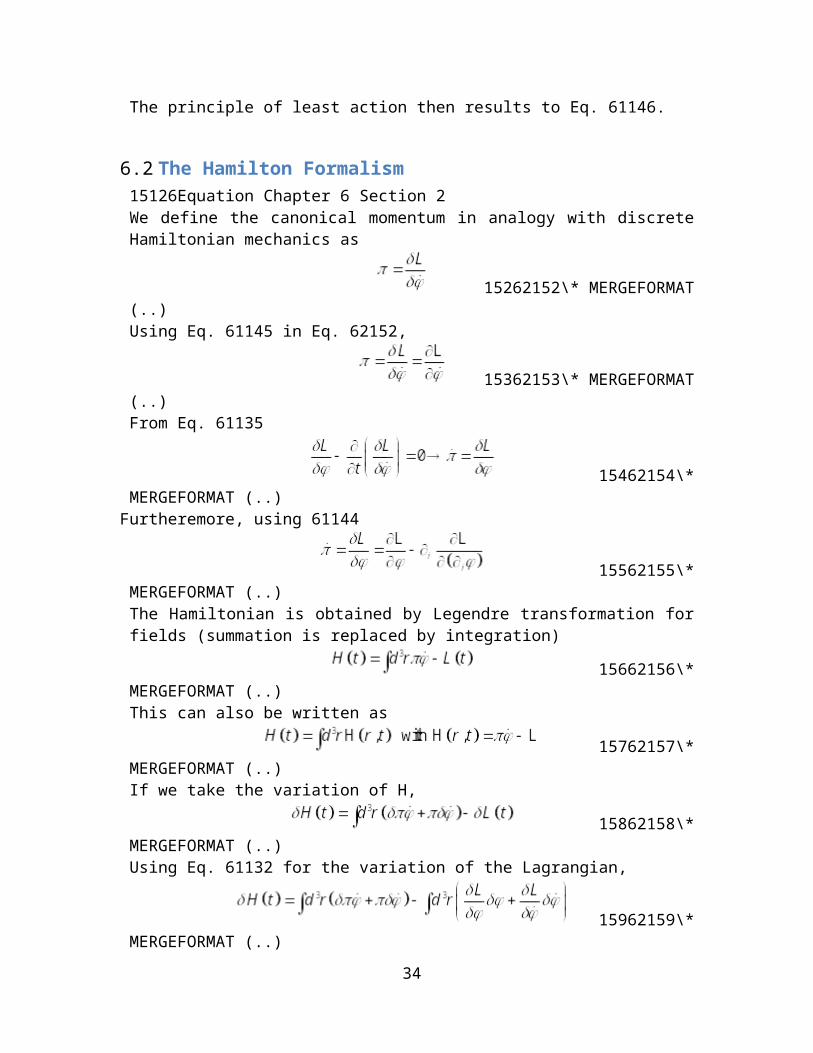
6.2 The Hamilton Formalism15126Equation Chapter 6 Section 2We define the canonical momentum in analogy with discrete Hamiltonian mechanics as
15262152\* MERGEFORMAT (..)Using Eq. 61145 in Eq. 62152,
15362153\* MERGEFORMAT(..)From Eq. 61135
15462154\*MERGEFORMAT (..)
Furtheremore, using 61144
15562155\*MERGEFORMAT (..)The Hamiltonian is obtained by Legendre transformation for fields (summation is replaced by integration)
15662156\*MERGEFORMAT (..)This can also be written as
15762157\*MERGEFORMAT (..)If we take the variation of H,
15862158\*MERGEFORMAT (..)
30
Using Eq. 61132 for the variation of the Lagrangian,
15962159\*MERGEFORMAT (..)and using Eqs. 62154 and 62152
16062160\*
MERGEFORMAT (..)Since the
16162161\*MERGEFORMAT (..)Comparing the above two equations, we obtain the Hamilton’s equations of motion,
16262162\* MERGEFORMAT (..)
16362163\* MERGEFORMAT(..)On the other hand, the variation of the Hamiltonian can be executed by using Eq. 62157 and noting that
Noting that and integrating by parts following Eqs. 61139-61142
16462164\* MERGEFORMAT (..)Comparing Eqs. 62161 and 62164
16562165\*MERGEFORMAT (..)
16662166\*MERGEFORMAT (..)The Hamilton’s equations of motion then become,
31
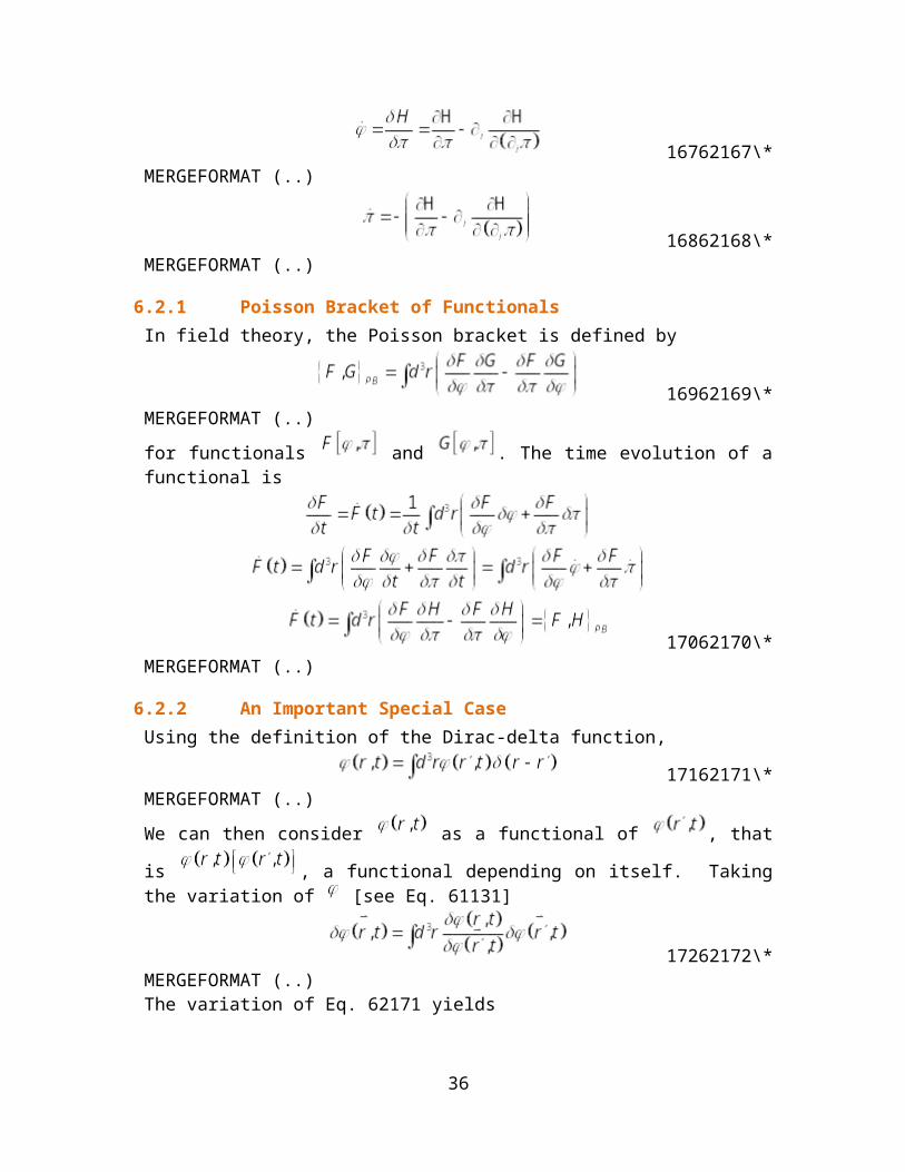
16762167\*MERGEFORMAT (..)
16862168\*MERGEFORMAT (..)
6.2.1 Poisson Bracket of FunctionalsIn field theory, the Poisson bracket is defined by
16962169\*MERGEFORMAT (..)for functionals and . The time evolution of a functional is
17062170\*MERGEFORMAT (..)
6.2.2 An Important Special CaseUsing the definition of the Dirac-delta function,
17162171\*MERGEFORMAT (..)We can then consider as a functional of , that is
, a functional depending on itself. Taking the variation of [see Eq. 61131]
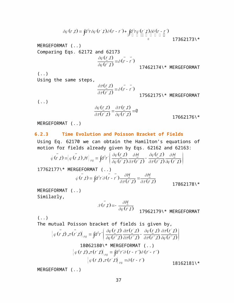
17262172\*MERGEFORMAT (..)The variation of Eq. 62171 yields
17362173\*MERGEFORMAT (..)Comparing Eqs. 62172 and 62173
32
17462174\*MERGEFORMAT (..)Using the same steps,
17562175\*MERGEFORMAT (..)
17662176\*MERGEFORMAT (..)
6.2.3 Time Evolution and Poisson Bracket of FieldsUsing Eq. 62170 we can obtain the Hamilton’s equations of motion for fields already given by Eqs. 62162 and 62163:
17762177\* MERGEFORMAT (..)
17862178\*MERGEFORMAT (..)Similarly,
17962179\*MERGEFORMAT (..)The mutual Poisson bracket of fields is given by,
18062180\* MERGEFORMAT (..)
18162181\*
MERGEFORMAT (..)and
18262182\*MERGEFORMAT (..)
6.3 Canonical Quantization18336Equation Chapter 6 Section 3
33
6.3.1 IntroductionThe following is taken from Chapter 3 of (Greiner & Reinhardt, 1996). See also Chapter 2 of (McMahon, 2008).
The process of transforming classical physical quantities into quantum mechanical operators and Poisson bracket into commutator is called first quantization. This process also results to the Schroedinger equation
18463184\*MERGEFORMAT (..)In the context of quantum field theory, the wavefunction can be considered as a complex classical field. We can then use the mathematical machinery introduced in Section 6.1 but in the inverse mode by searching for a Lagrangian density that will result to the Schroedinger equation 63184. It turns out that the appropriate Lagrangian density that will result to the Schroedinger equation (Greiner & Reinhardt, 1996) is
18563185\* MERGEFORMAT (..)with
This can be verified by substituting 63185 into Eq. 61147 with and
considered as independent fields:
18663186\* MERGEFORMAT (..)
18763187\* MERGEFORMAT (..)Let us write 63185 in the form,
34

18863188\* MERGEFORMAT (..)
Working on Eq. 63186
18963189\* MERGEFORMAT(..)
19063190\* MERGEFORMAT(..)
19163191\*MERGEFORMAT (..)Similarly,
19263192\*MERGEFORMAT (..)
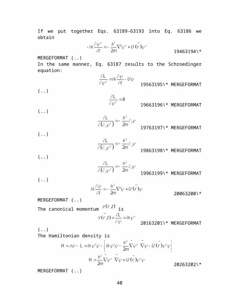
19363193\*MERGEFORMAT (..)If we put together Eqs. 63189-63193 into Eq. 63186 we obtain
19463194\*MERGEFORMAT (..)In the same manner, Eq. 63187 results to the Schroedinger equation:
19563195\*MERGEFORMAT (..)
19663196\* MERGEFORMAT (..)
19763197\*MERGEFORMAT (..)
35
19863198\*MERGEFORMAT (..)
19963199\*MERGEFORMAT (..)
20063200\*MERGEFORMAT (..)The canonical momentum is
20163201\*MERGEFORMAT (..)The Hamiltonian density is
20263202\*MERGEFORMAT (..)The Hamiltonian can be determined in the following:
20363203\*MERGEFORMAT (..)The first integral can be evaluated by integration by parts using the identity
20463204\* MERGEFORMAT (..)
Using divergence theorem to the first integral
The surface integral vanishes since the wavefunction decreases rapidly at the surface
36
20563205\* MERGEFORMAT (..)
6.3.2 Quantization Rules for Bosons
We quantize the fields and by promoting them into operators and , respectively. In this context the fields
and are considered classical fields. However, we already know that itself is a wavefunction, which is the by-product of quantizing classical physical quantities into operators. This transformation of physical quantities into operators is called first quantization while the quantization of and into field operators and , respectively, is called second quantization. Moreover, the Poisson brackets becomes commutators divided by
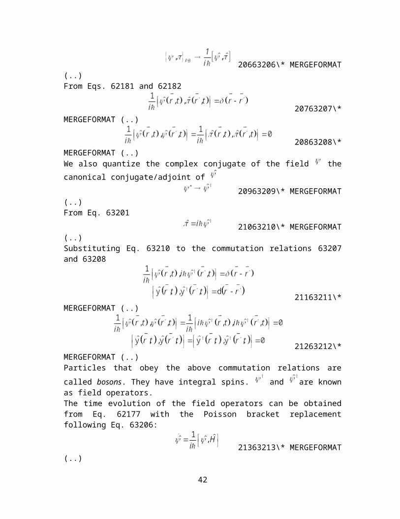
20663206\*MERGEFORMAT (..)From Eqs. 62181 and 62182
20763207\*MERGEFORMAT (..)
20863208\*MERGEFORMAT (..)We also quantize the complex conjugate of the field the canonical conjugate/adjoint of
20963209\* MERGEFORMAT (..)From Eq. 63201
21063210\* MERGEFORMAT (..)Substituting Eq. 63210 to the commutation relations 63207 and 63208
21163211\*
MERGEFORMAT (..)
37

21263212\*
MERGEFORMAT (..)Particles that obey the above commutation relations are called bosons. They have integral spins. and are known as field operators. The time evolution of the field operators can be obtained from Eq. 62177 with the Poisson bracket replacement following Eq. 63206:
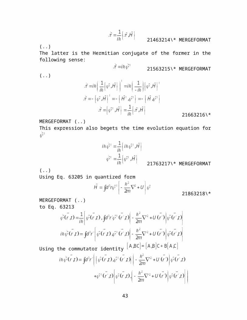
21363213\* MERGEFORMAT(..)
21463214\* MERGEFORMAT(..)The latter is the Hermitian conjugate of the former in the following sense:
21563215\* MERGEFORMAT (..)
21663216\*MERGEFORMAT (..)This expression also begets the time evolution equation for
21763217\* MERGEFORMAT(..)Using Eq. 63205 in quantized form
21863218\*MERGEFORMAT (..)to Eq. 63213
38

Using the commutator identity
21963219\*MERGEFORMAT (..)The time evolution of is given by the Schroedinger equation. However, this equation is now a derived equation not a postulate unlike the Schroedinger equation for the wavefunction in first quantization.In the same way,
39
22063220\*MERGEFORMAT (..)after an integration by parts. It turns out that this equation is the Hermitian conjugate of Eq. 63219.
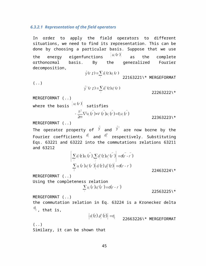
6.3.2.1 Representation of the field operators
In order to apply the field operators to different situations, we need to find its representation. This can be done by choosing a particular basis. Suppose that we use the energy eigenfunctions as the complete orthonormal basis. By the generalized Fourier decomposition,
22163221\*MERGEFORMAT (..)
22263222\*MERGEFORMAT (..)where the basis satisfies
22363223\*MERGEFORMAT (..)The operator property of and are now borne by the Fourier coefficients and respectively. Substituting Eqs. 63221 and 63222 into the commutations relations 63211 and 63212
22463224\*MERGEFORMAT (..)Using the completeness relation
22563225\*MERGEFORMAT (..)the commutation relation in Eq. 63224 is a Kronecker delta , that is,
22663226\* MERGEFORMAT(..)Similary, it can be shown that
40

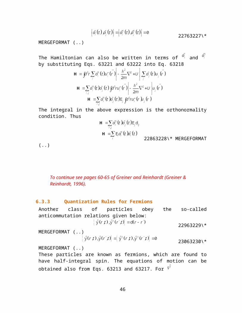
22763227\*MERGEFORMAT (..)
The Hamiltonian can also be written in terms of and by substituting Eqs. 63221 and 63222 into Eq. 63218
The integral in the above expression is the orthonormality condition. Thus
22863228\*MERGEFORMAT (..)
To continue see pages 60-65 of Greiner and Reinhardt (Greiner & Reinhardt, 1996).
6.3.3 Quantization Rules for FermionsAnother class of particles obey the so-called anticommutation relations given below:
22963229\*MERGEFORMAT (..)
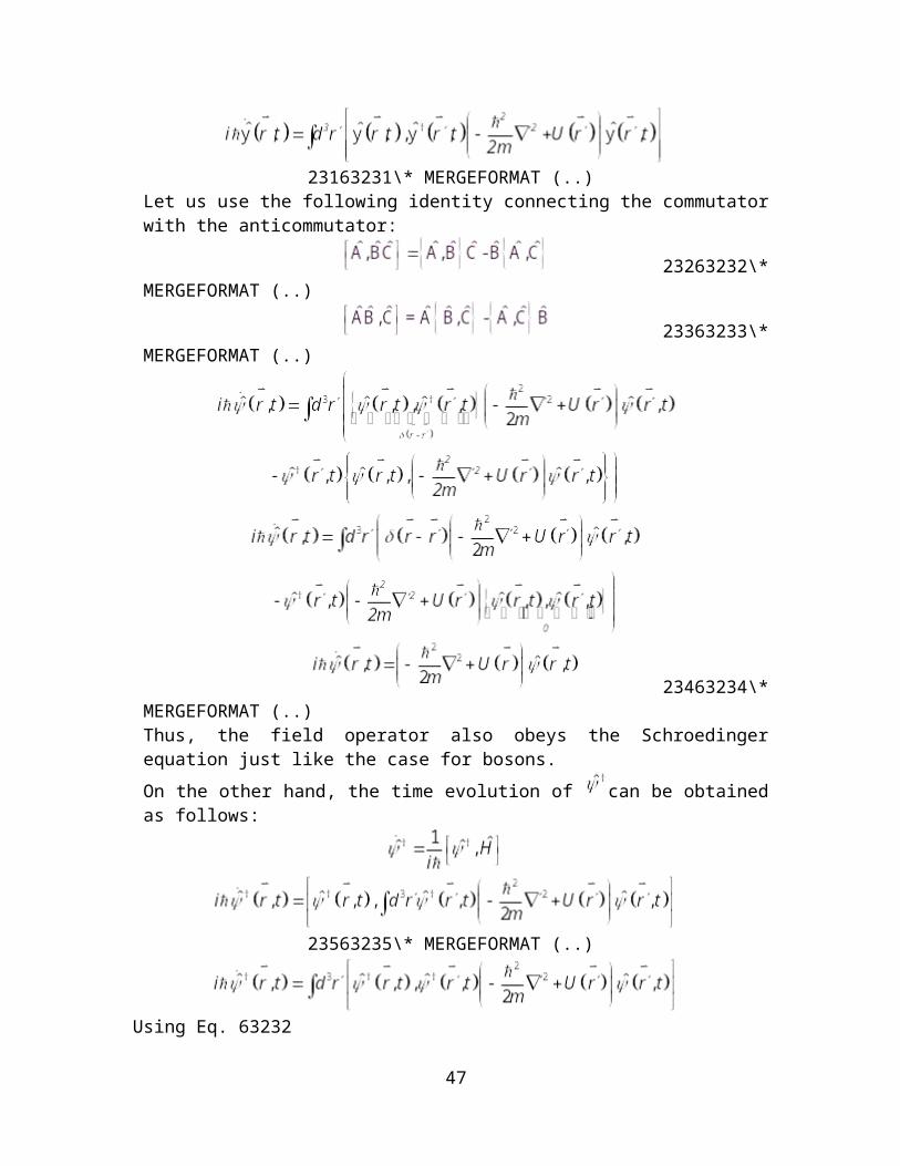
23063230\*MERGEFORMAT (..)These particles are known as fermions, which are found to have half-integral spin. The equations of motion can be obtained also from Eqs. 63213 and 63217. For
23163231\* MERGEFORMAT (..)
Let us use the following identity connecting the commutator with the anticommutator:
41
23263232\*MERGEFORMAT (..)
23363233\*MERGEFORMAT (..)
23463234\*MERGEFORMAT (..)Thus, the field operator also obeys the Schroedinger equation just like the case for bosons.On the other hand, the time evolution of can be obtained as follows:
23563235\* MERGEFORMAT (..)
Using Eq. 63232
42
After integration by parts,
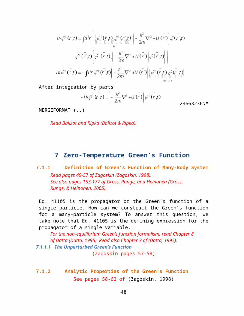
23663236\*MERGEFORMAT (..)
Read Balizot and Ripka (Balizot & Ripka).
7 Zero-Temperature Green’s Function
7.1.1 Definition of Green’s Function of Many-Body SystemRead pages 49-57 of Zagoskin (Zagoskin, 1998).See also pages 153-177 of Gross, Runge, and Heinonen (Gross, Runge, & Heinonen, 2005).
Eq. 41105 is the propagator or the Green’s function of a single particle. How can we construct the Green’s function for a many-particle system? To answer this question, we take note that Eq. 41105 is the defining expression for the propagator of a single variable.
For the non-equilibrium Green’s function formalism, read Chapter 8 of Datta (Datta, 1995). Read also Chapter 3 of (Datta, 1995).
7.1.1.1 The Unperturbed Green’s Function(Zagoskin pages 57-58)
7.1.2 Analytic Properties of the Green’s FunctionSee pages 58-62 of (Zagoskin, 1998)
7.1.2.1 Poles of Green’s Function and Quasiparticle Excitations
See page 62 of (Zagoskin, 1998)
7.1.3 Retarded and Advanced Green’s Function7.1.3.1 Quasiparticle Excitations and Advanced and Retarded Green’s Functions
7.2 Quantum Correlation Functions in Many-Body Theory
43

Click this link
7.3 Perturbation Theory: Feynman DiagramsSee page 66 of (Zagoskin, 1998)
8 Quantum Superfield Theory
The complete theoretical description of open, nonequilibrium systems is still an open problem in many-particle physics. The practical importance of this subject is more apparent in the studies of quantum transport in nanostructures. Most of the current theoretical and computational researches in the study of nanostructures and their device applications rely on conventional equilibrium transport techniques or near equilibrium quantum transport physics at best. If ever an attempt to analyze nonequilibrium quantum tranport is done, nonequilibrium Green’s function technigue is usually adopted (Kadanoff & Baym, 1962; Mahan G. D., 1990), which leads to the quantum Boltzmann equation. This technique however suffers from a serious drawback when applied to nanoscale structures, where there is an abrupt variation of physical quantities. The resulting transport equations are expressed in gradient expansion, which is applicable only for slow spatial variation of physical quantities and slow temporal variation of the fields. The formalism is also not applicable to describe ultrafast processes in nanodevices. Therefore, a wide spectrum of novel highly nonlinear, nonequilibrium quantum transport phenomena in nanostructures is not captured and their full application potentials for new functionalities are not realized. In this article we use quantum superfield theory(QSFT) combined with lattice Weyl transform techniques in solid-state physics. In QSFT, ordinary quantum field operators become superoperators while the von Neumann density operator evolution equation in Hilbert-Fock space becomes super-statevector quantum dynamical equation in Liouville space .
Notes:Read Arimitsu and Umezawa (Arimitsu & Umezawa, 1987; Arimitzu &Umezawa, 1987).Read Section 29.1 of Buot (Buot F. A., 2009).Read Chapter 8 of Datta (Datta, 1995) for a clear exposition of the nonequilibrium Green’s function.
44
8.1 Basic Concepts in Quantum Superfield Theory23713Equation Chapter 3 Section 1
8.1.1 Single-Particle9In quantum mechanics, the state of a particle is represented by a state vector in Hilbert space while physical quantities are represented by operators acting on . These operators also constitute a linear vector space, called the Liouville space attached to . An element in , which is an operator10 in , is denoted by
and known as superstate vector. Recall that we can also construct an operator in by the outer product or dyad formed by the state vectors and as follows,
23831238\* MERGEFORMAT (..)In Liouville space this should become a superstate vector denoted by
23931239\* MERGEFORMAT (..)Similarly, we can write the dyad formed by the orthonormal basis as a superstate vector in as
24031240\* MERGEFORMAT(..)Now recall that an operator in can be expressed in dyad decomposition as
24131241\*MERGEFORMAT (..)The corresponding superstate vector is written as
24231242\*MERGEFORMAT (..)
The set therefore span the Liouville space. We also anticipate that the superstate vectors in the set are linearly
9This discussion is based on Schmutz (Schmutz, 1978) and Section 1.2 of Audretsch (Audretsch, 2007).10 An operator in Hilbert space is written in bold.
45
independent11, which implies that the set constitutes a basis in . If the number of state vectors in the basis12 is , then the number
of superstate vectors in the set is . The dimension of is therefore . By definition, is itself a Hilbert space and is therefore endowed with an inner product. We define the inner as
24331243\* MERGEFORMAT(..)with the Hilbert-Schmidt norm given by
24431244\* MERGEFORMAT(..)The following requirements:
24531245\*MERGEFORMAT (..)
24631246\*MERGEFORMAT (..)
24731247\*MERGEFORMAT (..)are satisfied by 31243. Let us use Eq. 31243 to determine the inner product of the basis set
:
24831248\*
MERGEFORMAT (..)
Thus, the basis set is an orthonormal set.
11 They are, in fact, orthonormal which will be shown later.12 The dimension of is .
46
For consistency of terminology, we call the basis set in Liouville space, superbasis set. In general, a superbasis may not be in dyadic
form . Suppose that is an orthonormal superbasis set. Any superstate vector can be written as a linear combination of the superstate vectors in the superbasis,
24931249\* MERGEFORMAT(..)Since , the coefficient can be written as,
25031250\* MERGEFORMAT(..)Substitution of Eq. 31250 back to Eq. 31249 results to the closure relation
25131251\* MERGEFORMAT(..)where is the identity operator in Liouville space. Operators in Liouville space are called superoperators denoted by and is an example, which is consequently called identity superoperator. The quantity should be a superoperator, the analogue of the dyad . We call this superoperator superdyad. Following Eq. 31250, the coeficient in in Eq. 31242 can be written as
25231252\*MERGEFORMAT (..)Using Eq. 31243 for the definition of the inner product in ,
25331253\* MERGEFORMAT
(..)which is indeed the formula for as can be seen from Eq. 31241. In
the superbasis , the closure relation is written as
47
25431254\*MERGEFORMAT (..)
8.1.2 Many-Body System: The Thermal Liouville SpaceIf we deal with a many-particle (or many-body system) the Hilbert space becomes the Hilbert-Fock space . We choose the orthonormal basis in which
25531255\*MERGEFORMAT (..)for fermions and
25631256\* MERGEFORMAT (..)
for bosons. The vectors are the eigenvectors of the
number operator ,25731257\*
MERGEFORMAT (..)From now on, we simply use to mean . The annihilation and creation operators and satisfy the (anti)commutation relations
25831258\* MERGEFORMAT(..)
25931259\*MERGEFORMAT (..)where
In this case, the Liouville space consists of operators in . The superbasis is written as
26031260\* MERGEFORMAT(..)
in analogy with in the single-particle case. To simplify the notation we simply write expression 31260 as,
48
26131261\* MERGEFORMAT(..)and
26231262\*MERGEFORMAT (..)The orthonormality and completeness relations can be written, respectively, as,
26331263\*MERGEFORMAT (..)
26431264\*MERGEFORMAT (..)In the same way as Eq. 31242, we can also expand an arbitrary
superstate vector in the basis
26531265\*MERGEFORMAT (..)in which following Eqs. 31252 and 31253
26631266\*MERGEFORMAT (..)The bra is the adjoint of the corresponding ket,
26731267\* MERGEFORMAT(..)
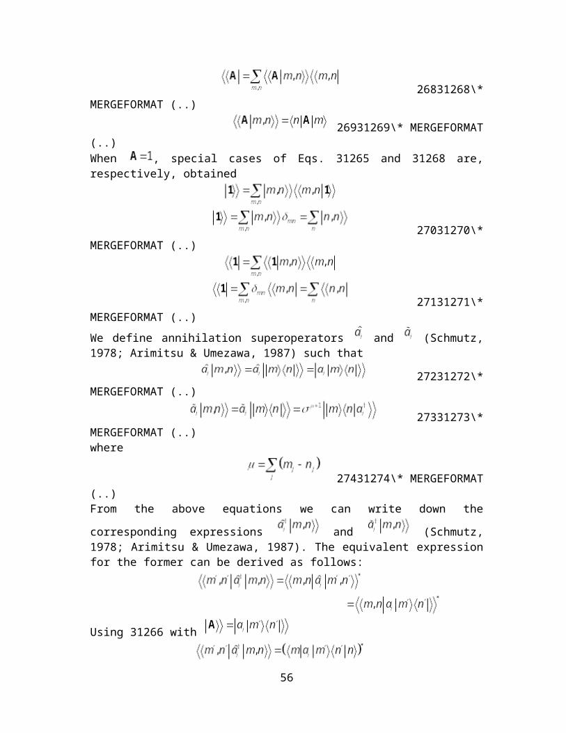
26831268\*MERGEFORMAT (..)
26931269\*MERGEFORMAT (..)When , special cases of Eqs. 31265 and 31268 are, respectively, obtained
27031270\*MERGEFORMAT (..)
49
27131271\*MERGEFORMAT (..)We define annihilation superoperators and (Schmutz, 1978;Arimitsu & Umezawa, 1987) such that
27231272\*MERGEFORMAT (..)
27331273\*MERGEFORMAT (..)where
27431274\* MERGEFORMAT(..)From the above equations we can write down the corresponding expressions and (Schmutz, 1978; Arimitsu &Umezawa, 1987). The equivalent expression for the former can be derived as follows:
Using 31266 with
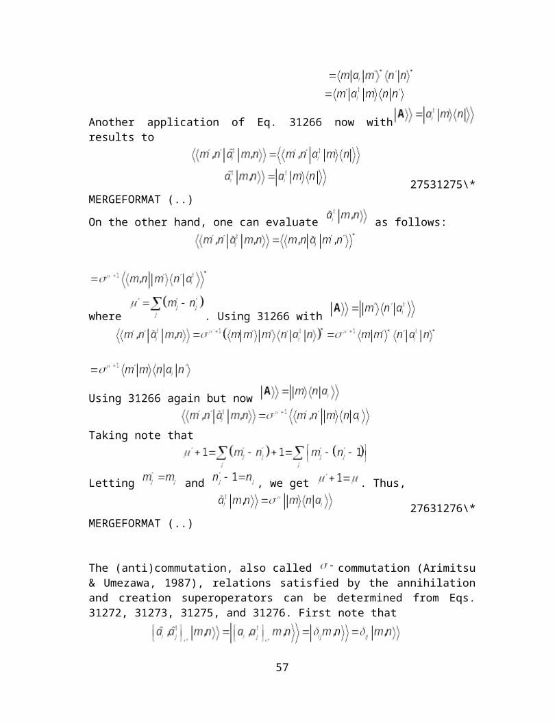
Another application of Eq. 31266 now with results to
27531275\*
MERGEFORMAT (..)On the other hand, one can evaluate as follows:
where . Using 31266 with
50
Using 31266 again but now
Taking note that
Letting and , we get . Thus,
27631276\*MERGEFORMAT (..)
The (anti)commutation, also called commutation (Arimitsu &Umezawa, 1987), relations satisfied by the annihilation and creation superoperators can be determined from Eqs. 31272, 31273, 31275, and 31276. First note that
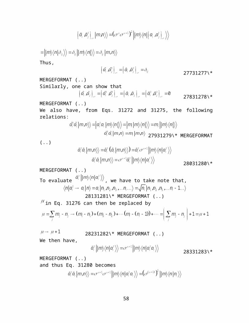
Thus,27731277\*
MERGEFORMAT (..)Similarly, one can show that
27831278\*MERGEFORMAT (..)We also have, from Eqs. 31272 and 31275, the following relations:
27931279\*
MERGEFORMAT (..)
28031280\*MERGEFORMAT (..)To evaluate , we have to take note that,
51
28131281\* MERGEFORMAT (..)in Eq. 31276 can then be replaced by
28231282\*MERGEFORMAT (..)We then have,
28331283\*MERGEFORMAT (..)and thus Eq. 31280 becomes
28431284\*MERGEFORMAT (..)We can also obviously have,
28531285\*MERGEFORMAT (..)where
28631286\* MERGEFORMAT(..)
is the supervacuum.The supervector can be constructed from the supervacuum using Eqs. 31255, 31256, and 31272-31278. For bosons, we have
28731287\*MERGEFORMAT (..)
52
28831288\*MERGEFORMAT (..)and for fermions, we also have
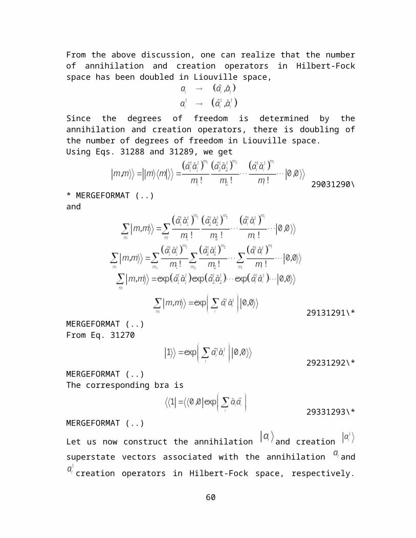
28931289\* MERGEFORMAT (..)From the above discussion, one can realize that the number of annihilation and creation operators in Hilbert-Fock space has been doubled in Liouville space,
Since the degrees of freedom is determined by the annihilation and creation operators, there is doubling of the number of degrees of freedom in Liouville space. Using Eqs. 31288 and 31289, we get
29031290\*MERGEFORMAT (..)and
29131291\*MERGEFORMAT (..)From Eq. 31270
53
29231292\*MERGEFORMAT (..)The corresponding bra is
29331293\*MERGEFORMAT (..)
Let us now construct the annihilation and creation superstate vectors associated with the annihilation and creation operators in Hilbert-Fock space, respectively. For the annihilation superstate vector, we note that from Eq. 31272,
29431294\*MERGEFORMAT (..)Thus, we can construct the annihilation supervector through Eq.31294
29531295\* MERGEFORMAT(..)We can also derive its alternative expression as,
29631296\* MERGEFORMAT(..)Thus, the annihilation superstate vector can be written in two forms:
29731297\* MERGEFORMAT(..)The creation superstate vector can be constructed using either Eq. 31295 or 31296 as follows:
29831298\* MERGEFORMAT(..)
54
29931299\* MERGEFORMAT(..)The creation superstate vector can be written in these forms:
30031300\*MERGEFORMAT (..)Continue here…..from page 36 of (Arimitsu & Umezawa, 1987).Suppose that A is an operator in . Upon second quantization, this operator takes a general form
30131301\*MERGEFORMAT (..)We define the superoperators
30231302\* MERGEFORMAT(..)
30331303\* MERGEFORMAT(..)where the complex conjugation sign is understood to be applied to the constant c. Let us now consider two arbitrary operators, A and B,
in . They become super-statevectors, and , in .The super-operators associated with A are given by Eqs. 31302 and 31303 while the super-statevectors can be written as a linear combination of the superbasis .
Given operators and , there exists an operator such that
30431304\* MERGEFORMAT(..)
30531305\* MERGEFORMAT(..)where
30631306\* MERGEFORMAT (..)To prove the first experssion, we have
55
This implies,30731307\* MERGEFORMAT
(..)The second one can be proven as follows,
30831308\* MERGEFORMAT(..)
30931309\*MERGEFORMAT (..)When , we have from Eqs.31307 and 31309,
31031310\* MERGEFORMAT (..)31131311\* MERGEFORMAT
(..)
For fermions,
31231312\*MERGEFORMAT (..)where . If the operator in Eq. 31301 conserves the fermion number, , and therefore
31331313\* MERGEFORMAT (..)
56
From Eqs. 31298 and 31299 one can also conclude that given a
superoperator in Liouville space, there exists an unique
operator such that,
31431314\*MERGEFORMAT (..)In the subsequent discussions, we assume that for fermions.
In the following, equations in Liouville space will be developed in terms of the field creation and annihilation superoperators , , , and .
8.2 Quantum Dynamics in Liouville Space31523Equation Chapter 3 Section 2Read Arimitzu and Umezawa (Arimitsu & Umezawa, 1987; Arimitzu &Umezawa, 1987). These two references introduced the quantum superfield theory.
8.2.1 Time Evolution EquationsIn conventional quantum mechanics, the state of a system is denoted
by a state ket, say or in the position representation by a
wavefunction . The density operator is then expressed in terms of the state ket or of the wavefunction. However, it is more convenient to consider the density or statistical operator as the fundamental quantity representing the state of the system. The state ket or the wavefunction can then be considered as derived quantity (Fain 2002). The (first) postulate in quantum mechanics, which states that (Tannoudji et al 1989):
“The state of a physical system at time t is represented by a state
ket .”
is replaced by the statement:
“The state of a physical system at time t is represented by a
density operator .”
57
The latter form of the first postulate is more appropriate in the QSFT formalism. Thus, the state of a physical system is represented by the density super-statevector
The expectation value of an operatorAin Hilbert-Fock space is written as (Blum, 1981)
31632316\* MERGEFORMAT(..)which can also be written as
31732317\* MERGEFORMAT(..)Using Eq. 31243, this can be written as
31832318\* MERGEFORMAT(..)Furthermore, we can invoke Eq. 31304 to write it in the form,
31932319\* MERGEFORMAT(..)where the superoperator is related to the operator according to Eq. 31302.
The time evolution of the density operator, and therefore of the state, is given by the von Neumann equation (Blum, 1981)
32032320\*MERGEFORMAT (..)where is the Hamiltonian. In converting this to the density super-statevector equation, we write
With the help of Eqs. 31304 and 31305,
32132321\*MERGEFORMAT (..)where is called the Liouvillian in analogy with the Hamiltonian :
32232322\* MERGEFORMAT (..)Eq. 32321 is called thesuper-Schroedinger equation in analogy with the Schroedinger equation in Hilbert-Fock space. We then say that the
58

system of bosons or fermions13 is characterized by the Liouvillian in the same way that a system of bosons or fermions is characterized by the Hamiltonian .
In arriving at Eq. 32321 we make use of the hermiticity of the Hamiltonian, that is,
32332323\* MERGEFORMAT (..)Eq. 32322 implies that
32432324\* MERGEFORMAT (..)
The corresponding density super-operator is constructed as follows:32532325\* MERGEFORMAT (..)
Note that
which satisfies Eq. 31314. In general, in constructing a superoperator in from an operator in we simply have14,
32632326\* MERGEFORMAT (..)
In analogy with Eqs. 32316 and 32319 we also define the expectation value of a super-operator as15
32732327\*MERGEFORMAT (..)It can also be shown that16
32832328\*MERGEFORMAT (..)
Let us now determine the time evolution equation of the density superoperator . From Eqs. 32321 and 32325,
32932329\*MERGEFORMAT (..)This equation can be written in a more suggestive form by noting that,
13 We can call them superbosons or superfermions.14 I am not sure of this. Justify this later.15 This is Eq. 3.8 of (Schmutz, 1978). Justify this expression later.16 I am not sure of this. Justify this later. This is Eq. (3.9) and (3.10) of (Schmutz,1978).
59
We can use this expression to show that33032330\* MERGEFORMAT
(..)Combining Eqs. 32329 and 32330,
33132331\*MERGEFORMAT (..)
8.2.2 The Unitary Superoperator
A unitary operator is defined by the relation33232332\* MERGEFORMAT
(..)In general, this operator is of the form
33332333\* MERGEFORMAT(..)
33432334\*MERGEFORMAT (..)where is a real number and is a Hermitian operator. The time evolution operator discussed in Section 2 is an example of a unitary operator. The construction of the corresponding unitary superoperator follows from Eqs. 31302 and 31303. Usually, can be written as
33532335\* MERGEFORMAT (..)Thus, using Eq. 32333
33632336\* MERGEFORMAT(..)
33732337\* MERGEFORMAT(..)
33832338\*MERGEFORMAT (..)Using Eq. 31310 and 31311
33932339\*MERGEFORMAT (..)
34032340\*MERGEFORMAT (..)We then have,
60
34132341\*MERGEFORMAT (..)
34232342\* MERGEFORMAT (..)
8.2.3 The Time Evolution Superoperator
We define the time evolution superoperator in analogy with Section 2. All the properties of the time evolution operator in Hilbert space should be satisfied by the time evolution superoperation in Liouville space. Being a unitary superoperator we expect that it can be written in the form 32335
34332343\* MERGEFORMAT (..)It is defined such that the superstatevector evolves as,
34432344\*MERGEFORMAT (..)In the same way that the wave function satisfies the Schroedinger’s equation 2125, the superstatevector satisfies the Liouville equation 32321. This gives us the differential equation
34532345\*MERGEFORMAT (..)for the time evoluton superoperator. This is of the same form as Eq. 2126 satisfied by the time evolution operator in Hilbert space.
In analogy with Eq. 2141, the general solution of Eq. 32345can be written as,
34632346\* MERGEFORMAT (..)which shows that,
34732347\* MERGEFORMAT (..)
61
34832348\*MERGEFORMAT (..)
34932349\*MERGEFORMAT (..)The fact that Eq. 32346 can be written in the form Eq. 32347is justified from the Campbell-Baker-Hausdorff identity (Buot F. A., 2009;Sakurai, 1994),
35032350\*MERGEFORMAT (..)wherein
35132351\* MERGEFORMAT (..)It also follows that
35232352\*MERGEFORMAT (..)In addition, Eqs. 32346 - 32349 obey Eqs. 31302 and 31303.
8.2.4 The Super-Heisenberg and Super-Interaction Pictures
In the Heisenberg representation, the state is not a function of time. We impose the same for the super-statevector. Thus,
35332353\* MERGEFORMAT(..)For
35432354\* MERGEFORMAT(..)In analogy with Eq. 2251, we define the super-Heisenberg representation of a superoperator as
35532355\*MERGEFORMAT (..)By direct differentiation with respect to time, it can be shown that this obeys the super-Heisenberg equation of motion,
35632356\*MERGEFORMAT (..)analogous to Eq. 2262. From Eq. 31310
62
With Eq. 32342,
35732357\* MERGEFORMAT(..)Using similar steps, it can also be shown that,
35832358\*MERGEFORMAT (..)In particular,
35932359\*MERGEFORMAT (..)
36032360\*MERGEFORMAT (..)
To define the super-interaction picture, we let36132361\* MERGEFORMAT (..)
following Eq. 2275. The relation between the super-statevector in the super-interaction picture to that in the Schroedinger picture is written as (see Eq. 2276),
36232362\* MERGEFORMAT (..)For the super-operator, we have the corresponding relation
36332363\*MERGEFORMAT (..)The time evolution of the supers-statevector can be obtained by time differentiation of Eq. 32362 making use of Eqs. 32345 and 32321 on the understanding that in the latter the super-statevector is in the Schroedinger picture and in the former should be replaced by . The result is
63
36432364\*MERGEFORMAT (..)where follows from the construction 32363. In the same way, from Eq. 32363
36532365\* MERGEFORMAT(..)The time evolution super-operator in the super-interaction picture follows from Eq. 32364:
36632366\*MERGEFORMAT (..)The solution of Eq. 32366 is obviously,
36732367\*MERGEFORMAT (..)In the same manner as in Section 3.3, it can be shown that,
36832368\*MERGEFORMAT (..)
One can also write in analogy with Eq. 2291 the equation,36932369\*
MERGEFORMAT (..)which gives the relation between super-operators in the super-Heisenberg and super-interaction pictures.
8.2.5 Super S-Matrix Theory and Variational Principle in Liouville Space8.2.5.1 Super S-Matrix Theory
Consider now the Liouvillian 32361. Let us interpret the second term as a perturbation that is turned on infinitely slowly at and that for times before the system is acted on by the unperturbed Liouvillian
only. This implies that the perturbation can be written as
37032370\*MERGEFORMAT (..)
64
where is an arbitrary initial time before .This type of thought experiment is called adiabatic turning on of state. Then in the Schroedinger picture we can write,
37132371\* MERGEFORMAT (..)For , the full Liouvillian acts and we have,
37232372\* MERGEFORMAT (..)We would like to express the above equations in the super-interaction picture. Following the prescription 32362
37332373\* MERGEFORMAT (..)Now substituting Eq. 32372, Eq. 32373 becomes,
37432374\*MERGEFORMAT (..)and with Eq. 32371 we finally obtain,
In the time interval , the interaction and the Schroedinger pictures coincide since the system is acted only by the unperturbed Liouvillian and so we have
37532375\*MERGEFORMAT (..)By defining the super S-matrix (in the super-interaction picture) as,
37632376\*MERGEFORMAT (..)This definition is reminiscent Eq. 32368. Eq. 32375then becomes
37732377\*MERGEFORMAT (..)
If we let and interpret , the latter being the equilibrium super-statevector, then Eq. 32377 becomes,
37832378\*MERGEFORMAT (..)
65
The left-hand side is the super-statevector at any time after the interaction has been switched on.
8.2.5.2 Time-Dependent Variational Principle in Liouville Space
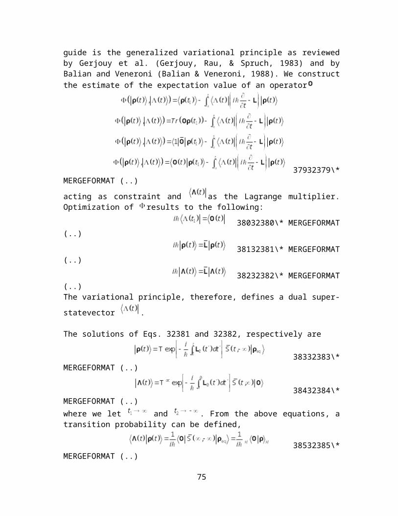
In quantum field theory, correlation functions are derived using variational principles. In this section let us explore the variational principle in Liouville space. Our guide is the generalized variational principle as reviewed by Gerjouy et al. (Gerjouy, Rau, & Spruch, 1983) and by Balian and Veneroni (Balian & Veneroni, 1988). We construct the estimate of the expectation value of an operator
37932379\*MERGEFORMAT (..)acting as constraint and as the Lagrange multiplier. Optimization of results to the following:
38032380\* MERGEFORMAT(..)
38132381\* MERGEFORMAT(..)
38232382\* MERGEFORMAT(..)The variational principle, therefore, defines a dual super-statevector
.
The solutions of Eqs. 32381 and 32382, respectively are
38332383\*MERGEFORMAT (..)
38432384\*MERGEFORMAT (..)
66
where we let and . From the above equations, a transition probability can be defined,
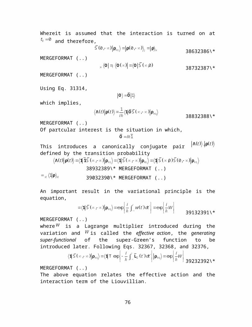
38532385\*MERGEFORMAT (..)Whereit is assumed that the interaction is turned on at and therefore,
38632386\*MERGEFORMAT (..)
38732387\*MERGEFORMAT (..)
Using Eq. 31314,
which implies,
38832388\*MERGEFORMAT (..)Of partcular interest is the situation in which,
This introduces a canonically conjugate pair defined by the transition probability
38932389\* MERGEFORMAT (..)39032390\* MERGEFORMAT (..)
An important result in the variational principle is the equation,
39132391\*MERGEFORMAT (..)where is a Lagrange multiplier introduced during the variation and
is called the effective action, the generating super-functional of the super-Green’s function to be introduced later. Following Eqs. 32367, 32368, and 32376,
39232392\*MERGEFORMAT (..)The above equation relates the effective action and the interaction term of the Liouvillian.
67
8.3 Super-Green’s Functions39343Equation Chapter 3 Section 4Let us introduce the 4-component second quantized quantum field super-operator
39434394\* MERGEFORMAT(..)where the argument is a short-hand notation for ; is a quantum number (or a set of quantum numbers).To identify the components of the 4-component field super-operator, we adopt the notation that represents its components, where . Thus we can have the following identification
39534395\* MERGEFORMAT(..)The commutation (anticommutation) relations of the 4-component field super-operator are the following:
39634396\*MERGEFORMAT (..)
39734397\*MERGEFORMAT (..)
39834398\*MERGEFORMAT (..)where
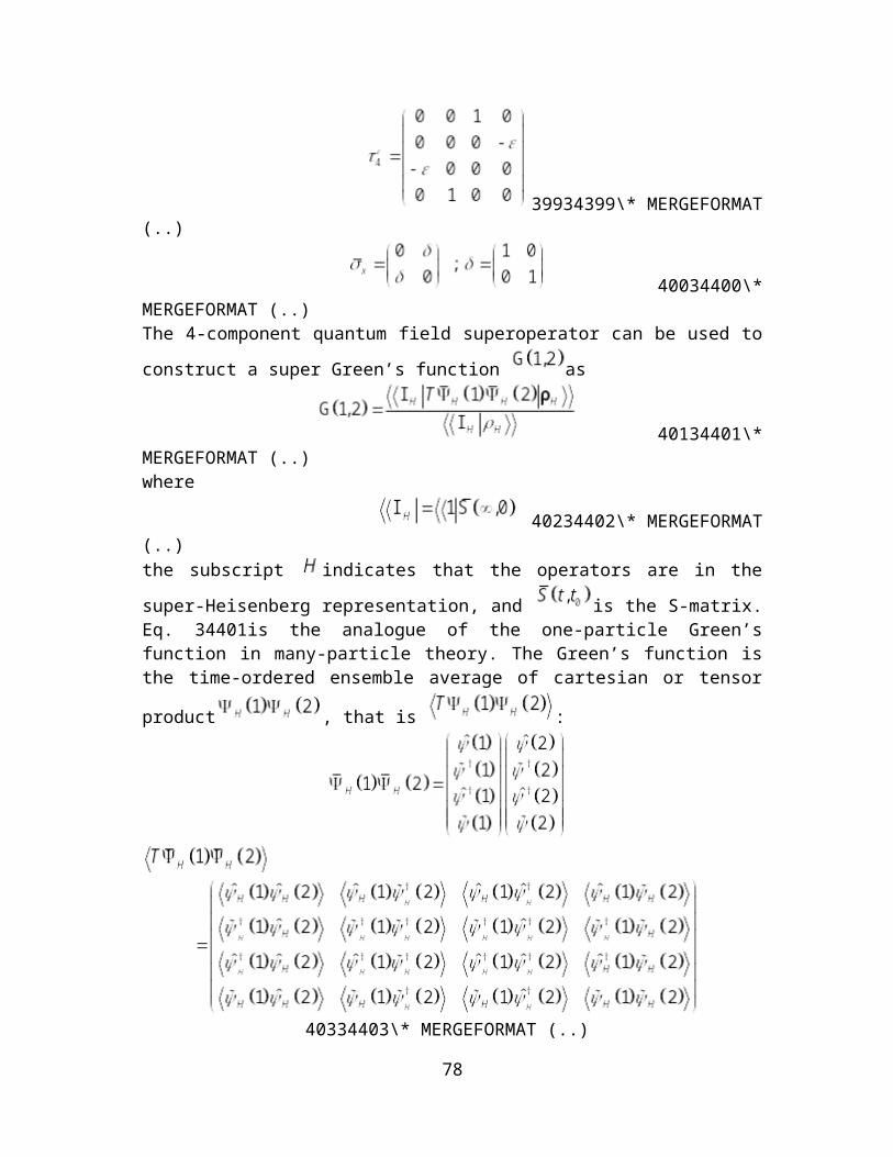
39934399\*MERGEFORMAT (..)
40034400\*MERGEFORMAT (..)
68
The 4-component quantum field superoperator can be used to construct a super Green’s function as
40134401\*MERGEFORMAT (..)where
40234402\*MERGEFORMAT (..)the subscript indicates that the operators are in the super-Heisenberg representation, and is the S-matrix. Eq. 34401is the analogue of the one-particle Green’s function in many-particle theory. The Green’s function is the time-ordered ensemble average of
cartesian or tensor product , that is :
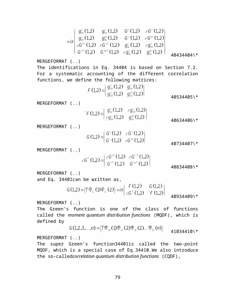
40334403\* MERGEFORMAT (..)
40434404\*MERGEFORMAT (..)The identifications in Eq. 34404 is based on Section 7.2. For a systematic accounting of the different correlation functions, we define the following matrices:
69

40534405\*MERGEFORMAT (..)
40634406\*MERGEFORMAT (..)
40734407\*MERGEFORMAT (..)
40834408\*MERGEFORMAT (..)and Eq. 34401can be written as,
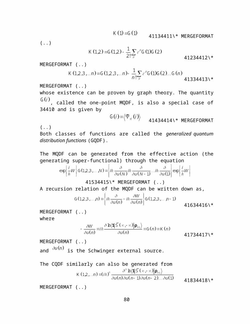
40934409\*MERGEFORMAT (..)The Green’s function is one of the class of functions called the moment quantum distribution functions (MQDF), which is defined by
41034410\*MERGEFORMAT (..)The super Green’s function34401is called the two-point MQDF, which is a special case of Eq.34410.We also introduce the so-calledcorrelation quantum distribution functions (CQDF),
41134411\* MERGEFORMAT(..)
41234412\*MERGEFORMAT (..)
41334413\*MERGEFORMAT (..)whose existence can be proven by graph theory. The quantity , called the one-point MQDF, is also a special case of 34410 and is given by
41434414\* MERGEFORMAT(..)
70
Both classes of functions are called the generalized quantum distribution functions (GQDF).
The MQDF can be generated from the effective action (the generating super-functional) through the equation
41534415\* MERGEFORMAT (..)A recursion relation of the MQDF can be written down as,
41634416\*MERGEFORMAT (..)where
41734417\*MERGEFORMAT (..)and is the Schwinger external source.
The CQDF similarly can also be generated from
41834418\*MERGEFORMAT (..)with the recursion relation
41934419\*MERGEFORMAT (..)
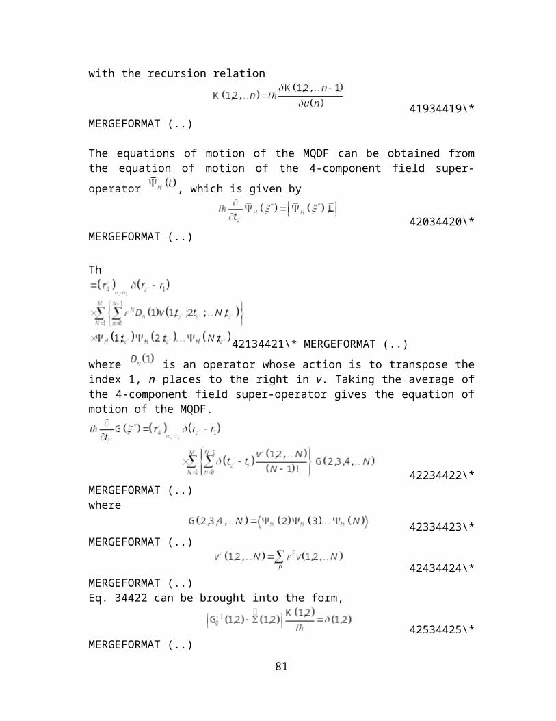
The equations of motion of the MQDF can be obtained from the equation of motion of the 4-component field super-operator , which is given by
42034420\*MERGEFORMAT (..)
Th
71

42134421\* MERGEFORMAT (..)where is an operator whose action is to transpose the index 1, n places to the right in v. Taking the average of the 4-component field super-operator gives the equation of motion of the MQDF.
42234422\*MERGEFORMAT (..)where
42334423\*MERGEFORMAT (..)
42434424\*MERGEFORMAT (..)Eq. 34422 can be brought into the form,
42534425\*MERGEFORMAT (..)where
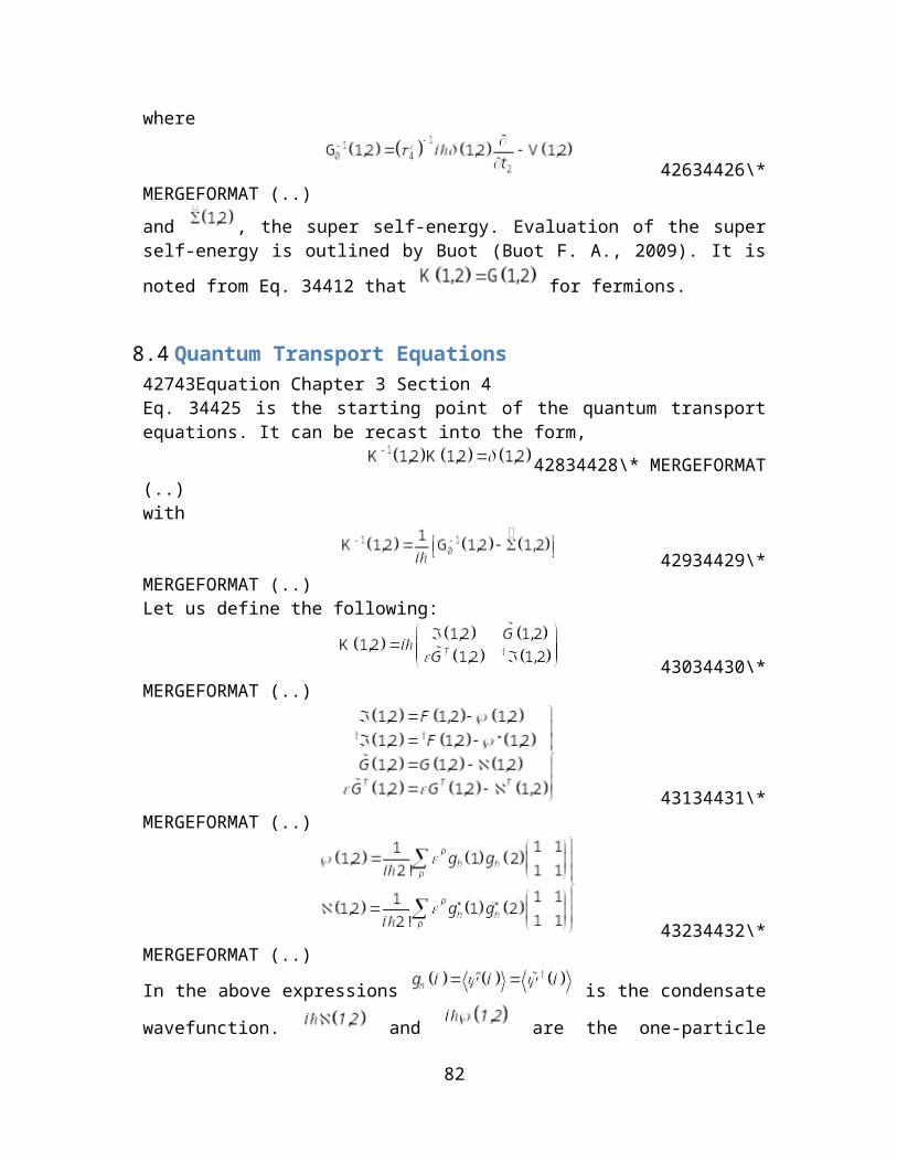
42634426\*MERGEFORMAT (..)and , the super self-energy. Evaluation of the super self-energy is outlined by Buot (Buot F. A., 2009). It is noted from Eq. 34412 that
for fermions.
8.4 Quantum Transport Equations42743Equation Chapter 3 Section 4Eq. 34425 is the starting point of the quantum transport equations. It can be recast into the form,
42834428\*MERGEFORMAT (..)with
42934429\*MERGEFORMAT (..)Let us define the following:
72
43034430\*MERGEFORMAT (..)
43134431\*MERGEFORMAT (..)
43234432\*MERGEFORMAT (..)In the above expressions is the condensate wavefunction. and are the one-particle reduced density matrix and the anomalous reduced density matrix of the boson condensate, respectively. They are zero for fermions.
8.5 Energy Band Dynamics of Bloch Electrons43353Equation Chapter 3 Section 5
8.5.1 Bloch and Wannier Functions
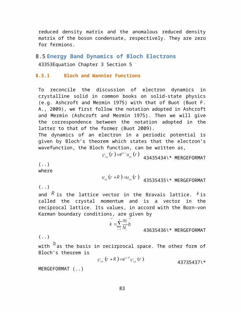
To reconcile the discussion of electron dynamics in crystalline solid in common books on solid-state physics (e.g. Ashcroft and Mermin 1975) with that of Buot (Buot F. A., 2009), we first follow the notation adopted in Ashcroft and Mermin (Ashcroft and Mermin 1975). Then we will give the correspondence between the notation adopted in the latter to that of the former (Buot 2009).The dynamics of an electron in a periodic potential is given by Bloch’s theorem which states that the electron’s wavefunction, the Bloch function, can be written as,
43435434\*MERGEFORMAT (..)where
43535435\*MERGEFORMAT (..)and is the lattice vector in the Bravais lattice. is called the crystal momentum and is a vector in the reciprocal lattice. Its values, in
73
accord with the Born-von Karman boundary conditions, are given by
43635436\* MERGEFORMAT(..)with as the basis in recirprocal space. The other form of Bloch’s theorem is
43735437\*MERGEFORMAT (..)To show consistency with Buot’s notation, we make the following substitution:
and replace the band index by . We also note that is the crystal momentum which justifies the above replacement and is the position variable. We also write,
If one keeps fixed, Bloch’s theorem implies that is a periodic function of . This means that can be expanded in Fourier series. Thus,
43835438\*MERGEFORMAT (..)The Fourier coefficient is called the Wannier function while
is obviously the Bloch function. Making use of the identity (actually the completeness relation of plane wave-basis in the lattice),
43935439\*MERGEFORMAT (..)we can derive the inverse relation,
44035440\*MERGEFORMAT (..)The steps leading to Eq. 35440 are the following:
74
With the use of Eq. 35439
Changing we obtain Eq. 35440.
We also take note of the orthogonality condition for the plane waves in the lattice,
44135441\*MERGEFORMAT (..)It is clear that the phase space variables are discrete.
In Dirac notation, the Bloch and Wannier functions can be written as44235442\* MERGEFORMAT
(..)44335443\* MERGEFORMAT
(..)where the basis kets (eigenkets) are given by:
44435444\* MERGEFORMAT(..)
44535445\* MERGEFORMAT(..)In the above equations we define the collective variable and
. The orthonormality relations are44635446\*
MERGEFORMAT (..)44735447\*
MERGEFORMAT (..)The completeness (closure) relationsare also given by17
17For continuous eigenvalues of the position and momentum, the summations are replaced by integrals.
75
44835448\*MERGEFORMAT (..)
44935449\*MERGEFORMAT (..)The transformation equation between the two bases is defined as,
45035450\*MERGEFORMAT (..)Using the closure relation 35448 and transformation equation 35450, we could have written Eq. 35438 as,
45135451\*MERGEFORMAT (..)The position representation of Eq. 35451 is Eq. 35438. The former equation can be interpreted in a more general point of view. It suggests two bases labeled by the band index and , and
labeled by the band index and , connected by a Fourier transformation. The wavefunctions and can then be considered as position representations of the general basis states
and , respectively, in which the Bloch and Wannier functions are special cases of these complete sets.
Likewise one can also have,
45235452\*MERGEFORMAT (..)
76

8.5.2 Lattice Weyl-Wigner Formulation of Electron Band Dynamics
Using the closure relations 35448 and 35449, any operator can be written as
45335453\*MERGEFORMAT (..)
45435454\* MERGEFORMAT (..)
Changing to one obtains,
45535455\*MERGEFORMAT (..)Introducing the notation,
45635456\*MERGEFORMAT (..)the above equation becomes
45735457\* MERGEFORMAT (..)with change to . Letting
45835458\*MERGEFORMAT (..)
45935459\*MERGEFORMAT (..)Eq. 35457 can be written as
77
46035460\*MERGEFORMAT (..)Using Eq. 35452, one can write the lattice-Weyl transform in alternative form. We first write down followingEq. 35452 in the form,
46135461\*MERGEFORMAT (..)
46235462\*MERGEFORMAT (..)Similarly, can be written as,
46335463\*MERGEFORMAT (..)Substituting Eq. 35463 into Eq. 35462, one obtains
46435464\* MERGEFORMAT (..)From Eq. 35441,
46535465\*MERGEFORMAT (..)Using the result 35465 into Eq. 35464,
78
46635466\*MERGEFORMAT (..)Replacing with ,
46735467\*MERGEFORMAT (..)Similarly, Eq. 35459 can be written in the form,
46835468\*MERGEFORMAT (..)using Eq. 35451 to write as,
and as,
46935469\*MERGEFORMAT (..)
is the lattice Weyl transform of the operator . One can also note that is an operator,in fact it is a projection operator. It is for this reason that we call it the phase-space point projector. Thus, Eq. 35460 means that an operator is expanded in terms of the phase-space point projector and that the expansion coefficients are the lattice-Weyl transform of . It has to be noted that the phase-space points are discrete. Thus, the operator is cast into discrete phase space by virtue of Eq. 35460. In summary, quantum mechanics can be cast into lattice (discrete) phase space by the bases and and the lattice-Weyl transformation of operator .
8.5.2.1 The Trace of an Operator
The representation of an operator in the form of Eq. 35460 is convenient in evaluating its trace.
79
47035470\*MERGEFORMAT (..)
47135471\*MERGEFORMAT (..)where we substitute Eq. 35460 for . Simplifying
Substituting Eq. 35459 for
47235472\*MERGEFORMAT (..)
In some applications, the trace of a product of operators is required. For each operator one can have, using Eq. 35460,
47335473\*MERGEFORMAT (..)
47435474\*MERGEFORMAT (..)The trace of is,
47535475\*MERGEFORMAT (..)
80
Note that
Continuing,
81
47635476\* MERGEFORMAT (..)But from Eq. 35439
47735477\*MERGEFORMAT (..)Thus, Eq. 35476 becomes
Implementing the change of variable,
gives the result
47835478\*MERGEFORMAT (..)
8.5.2.2 The Lattice-Weyl Transform of Product of Operators
The lattice-Weyl transform of the product of operators can be written using either Eq. 35458or Eq. 35467. Thus we have, respectively,
47935479\*MERGEFORMAT (..)
48035480\*MERGEFORMAT (..)We write the operators and as in Eq. 35460:
48135481\*MERGEFORMAT (..)
82
48235482\*MERGEFORMAT (..)If we use Eq. 35479 to evaluate the lattice-Weyl transform, we should use Eq. 35468 for . On the other hand, if we use Eq. 35480 to evaluate the lattice-Weyl transform, we should use Eq. 35459 for .Following the latter scheme,
48335483\*MERGEFORMAT (..)Using Eq. 35459 for the
48435484\*MERGEFORMAT (..)
48535485\*MERGEFORMAT (..)Thus, one can have
83

48635486\*MERGEFORMAT (..)Substiuting the above equation to Eq. 35483
48735487\*MERGEFORMAT (..)The bracketed quantity in the exponent can be written as
Letting and , we obtain
Substituting the above expression to Eq. 35487, one gets84

48835488\* MERGEFORMAT (..)A simplification of the above equation can be carried out if we assume that there are two continuous functions of and such that they are equal to and at each lattice point. Thus, we are justified in performing a Taylor series expansion of about ,
48935489\*MERGEFORMAT (..)
where and . Eq. 35488then becomes,
49035490\*MERGEFORMAT (..)To simplify things further, we note that
Thus, we may write Eq. 35490 as
49135491\*MERGEFORMAT (..)where the left arrows indicate that the derivative acts on the left, that is on the exponential function, while the right arrows indicate derivatives acting on .
85
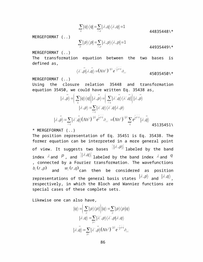
Using Eqs. 35439 and 35441,
49235492\* MERGEFORMAT (..)Using another notation,
49335493\* MERGEFORMAT (..)The superscript in the derivative operator means that it acts on
. If we consider the Weyl transforms as matrices, with the elements determined by the band indices, that is, the band indices as row and column indices, one can see that the summation over together with the indices and implies matrix multiplication. In matrix form, Eq. 35493 can then be written as
49435494\* MERGEFORMAT (..)
8.5.2.3 The Lattice-Weyl Transform of the Commutator and the Anticommutator of Operators
For the commutator:49535495\*
MERGEFORMAT (..)In matrix form:
86
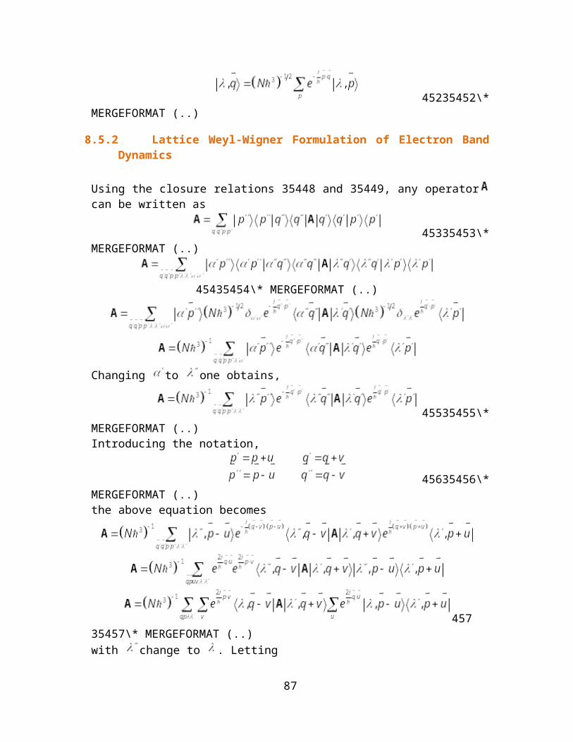
49635496\*MERGEFORMAT (..)Take note that the second exponential operator can be written as
Thus,
49735497\* MERGEFORMAT (..)
For the anticommutator:
87
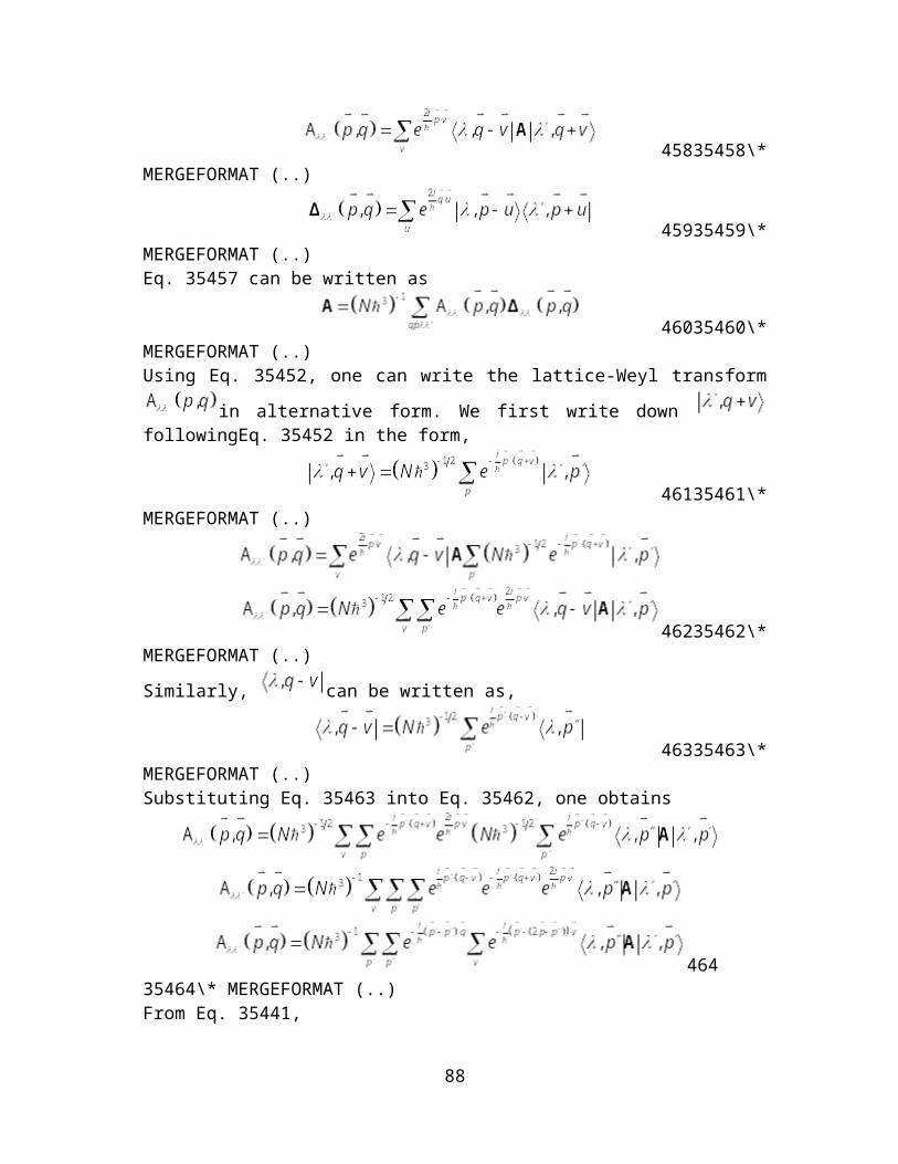
49835498\*MERGEFORMAT (..)In matrix form
49935499\* MERGEFORMAT(..)
50035500\* MERGEFORMAT (..)
88

8.5.3 Weyl Transformation in Continuous Phase Space
For the sake of completeness we discuss in this section the Weyl transformation in continuous phase space. Another reason for discussing it is that in actual calculation, we will be adopting the continuous phase-space approximation. The closure relation for continuous and are given by
50135501\*MERGEFORMAT (..)
50235502\*MERGEFORMAT (..)where it is understood that
50335503\* MERGEFORMAT(..)Recall also that
50435504\*MERGEFORMAT (..)The analog of the completeness relation 35439 can be obtained from Eq. 35501,
50535505\*MERGEFORMAT (..)The orthogonality in the Dirac sense is also given by
89
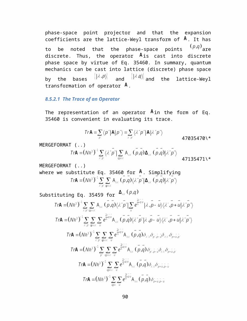
50635506\*MERGEFORMAT (..)
We also note that the position eigenkets can be written as,
50735507\*MERGEFORMAT (..)Using Eq. 35504
50835508\*MERGEFORMAT (..)Similarly,
50935509\*MERGEFORMAT (..)
51035510\*MERGEFORMAT (..)
Any operator can then be written in the form
Using Eq. 35504
90
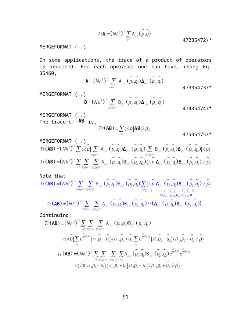
51135511\* MERGEFORMAT (..)We introduce the new variables
51235512\*MERGEFORMAT (..)and to , so that the above equation can be written as,
51335513\*MERGEFORMAT (..)Defining,
51435514\*MERGEFORMAT (..)
51535515\*MERGEFORMAT (..)Eq. 35513 can be written as,
51635516\*MERGEFORMAT (..)We can also write this in the form
91
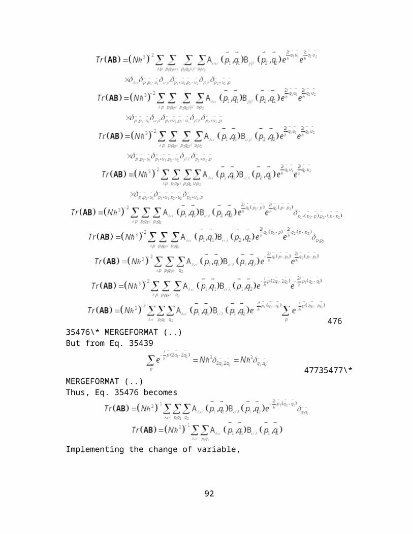
51735517\*MERGEFORMAT (..)
using the notation .
The Weyl transform can also be written in terms of the momentum by making use of Eq. 35508. We write
51835518\*MERGEFORMAT (..)Likewise,
51935519\*MERGEFORMAT (..)Thus, Eq. 35514 can be written as,
Letting
92
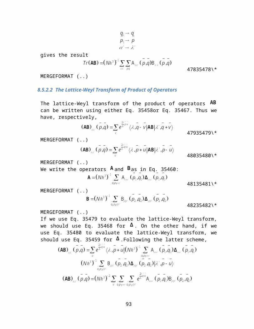
Since the integrand is evaluated over all the momentum space, the negative sign has no effect on the integral. Thus,
52035520\*MERGEFORMAT (..)Similarly, using similar steps,
52135521\*MERGEFORMAT (..)
8.5.3.1 The Trace of an Operator in Continuous Phase Space
The trace of an operator can be written in terms of the basis or
. Using the latter,
52235522\*MERGEFORMAT (..)Inserting expression 35516 or 35517 for
Note that,
52335523\* MERGEFORMAT (..)Using Eq. 35515 for ,p qΔ
,
93

52435524\*MERGEFORMAT (..)For single band, this becomes
52535525\*MERGEFORMAT (..)
The trace of the product of operators is given by
52635526\*MERGEFORMAT (..)We can use Eq. 35516 to write and as follows:
52735527\*MERGEFORMAT (..)
52835528\*MERGEFORMAT (..)and the becomes
94

Take note that,
Now the ’s can be written as follows, using Eq. 35515:
52935529\*MERGEFORMAT (..)
53035530\*MERGEFORMAT (..)
Simplifying the summations,
95

We can now simplify the integrations:
To evaluate the integral with as the variable, we let
96
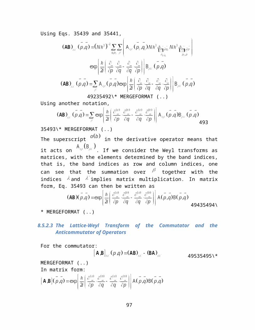
We also let to evaluate the integral over .
In the same manner we can also let to evaluate the integral over
Take note that the exponent can be written as:
The integral over can be evaluated by letting :
97
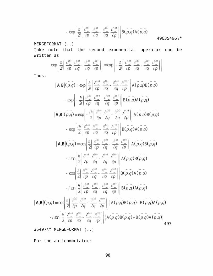
Changing the variables ,
53135531\*MERGEFORMAT (..)For a single band,
53235532\*MERGEFORMAT (..)
8.5.3.2 Weyl Transform of Product of Operators in Continuous Phase Space
We follow the similar steps as in the previous section, using Eq. 35514 to write the Weyl transform as follows,
53335533\*MERGEFORMAT (..)One can also write the Weyl transform using the Eq. 35520
53435534\*MERGEFORMAT (..)We also write the individual operators using Eq. 35516 in the form,
53535535\*MERGEFORMAT (..)
53635536\*MERGEFORMAT (..)
98
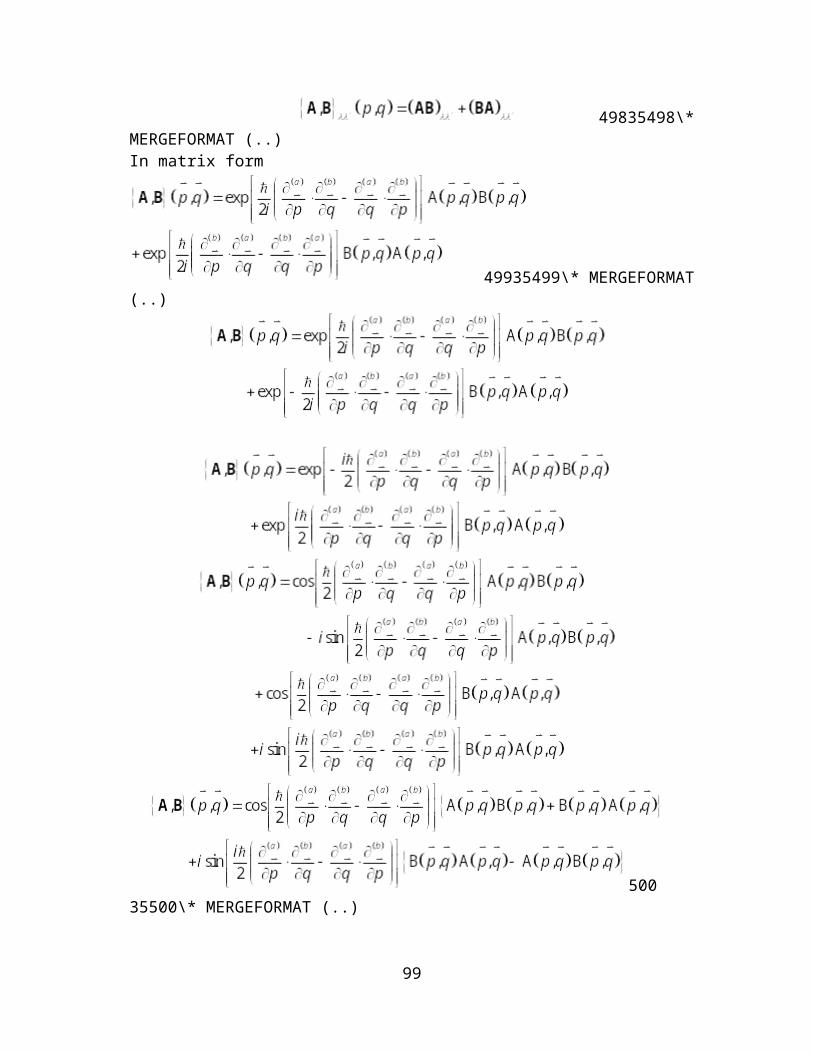
In evaluating the Weyl transform of the product of operators, we can use either use Eq. 35533 together with Eq. 35521 for the ’s or use Eq. 35534 together with Eq. 35515 for the ’s. We follow the latter so that
53735537\*MERGEFORMAT (..)Let us first consider the quantity,
. We use Eq. 35515 for the ’s:
53835538\*MERGEFORMAT (..)
53935539\*MERGEFORMAT (..)
99
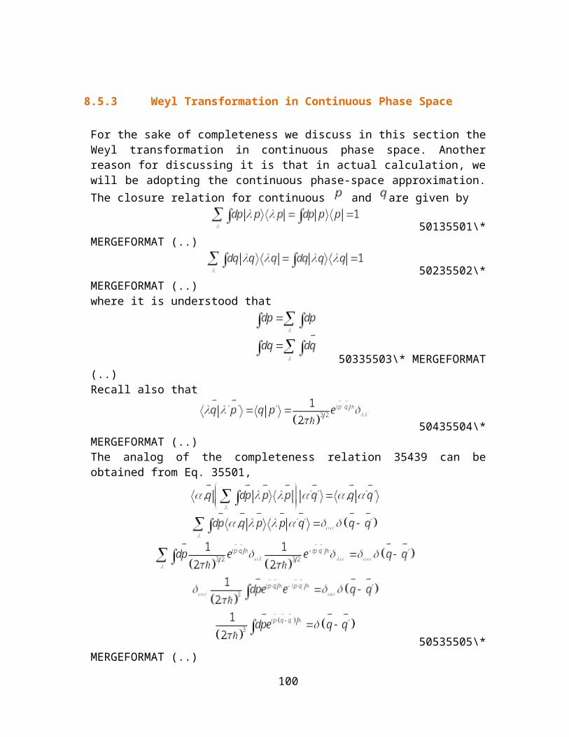
54035540\*MERGEFORMAT (..)Substituting Eq. 35540 to Eq. 35537
100
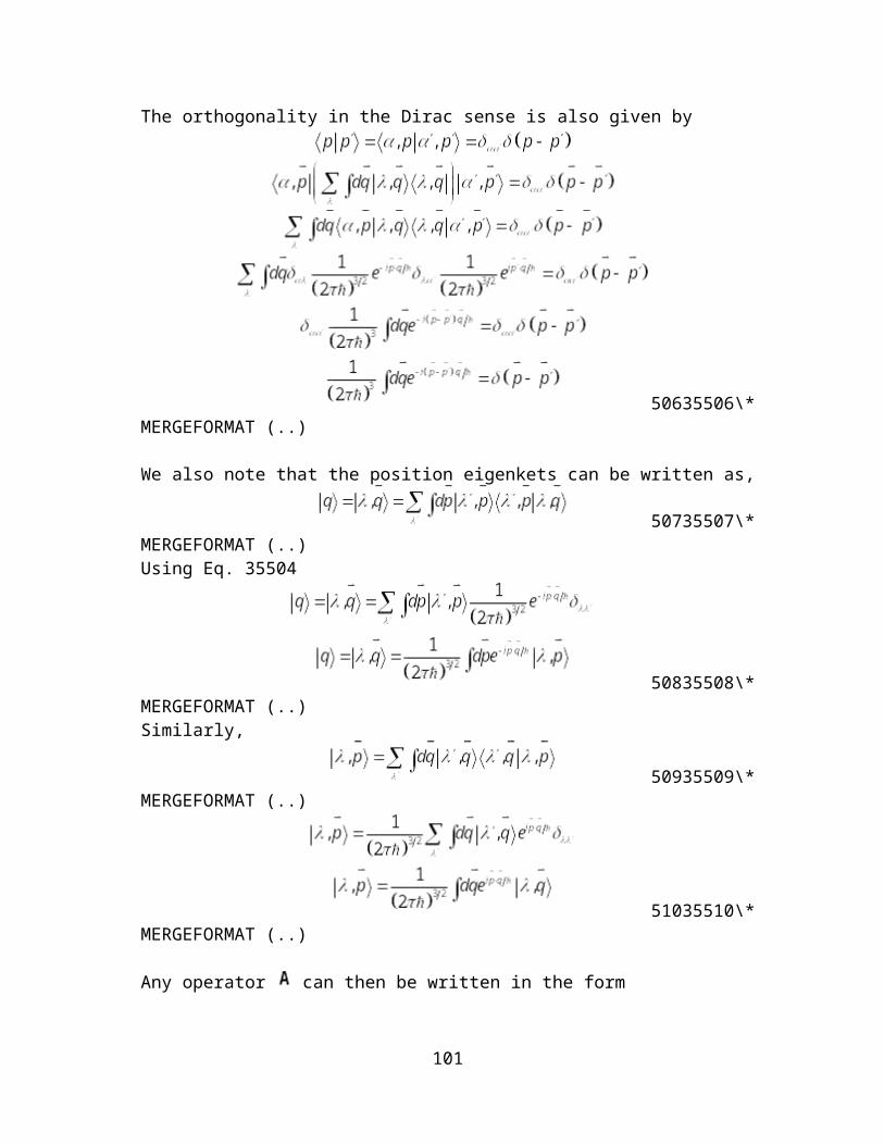
54135541\*MERGEFORMAT (..)The exponent in Eq. 35541 is exactly the same as in Eq. 35487. Using similar steps we arrive at an expression the same as Eqs. 35493 and 35494. For the single-band case
54235542\* MERGEFORMAT (..)
8.5.3.3 Weyl Transform of Commutator and Anticommutator of Operators
The formulas for the commutator and anticommutator turn out to be the same as Eqs. 35497 and 35500, respectively. For a single band using Eq. 35542, we have
54335543\* MERGEFORMAT (..)Similarly, for the anticommutator,
54435544\* MERGEFORMAT (..)
101
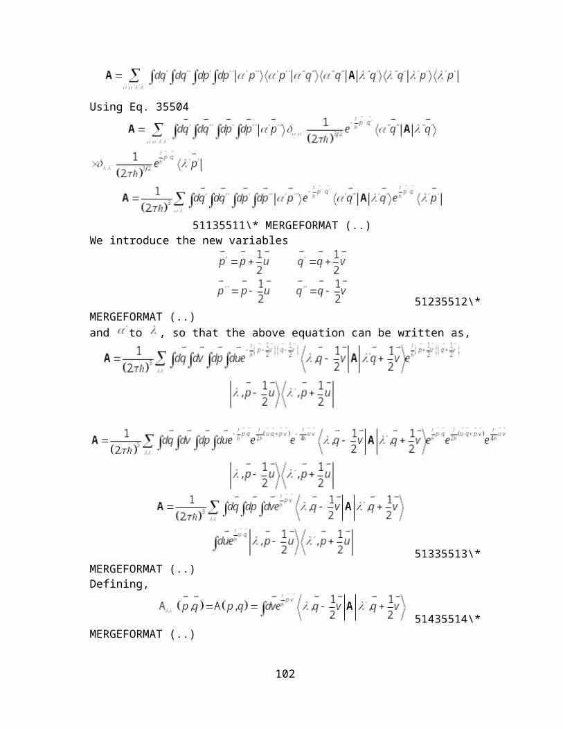
8.5.4 Integral Form of the Weyl Transform of the Commutator and Anticommutator
Usually, it is more convenient computationally if the Weyl transform of the commutator and the anticommutator are written in integral from. These forms can be derived from the corresponding differential form by using the displacement operator. The results are:
54535545\*MERGEFORMAT (..)
54635546\* MERGEFORMAT (..)
54735547\* MERGEFORMAT (..)where
54835548\* MERGEFORMAT (..)For scalar functions,
54935549\*MERGEFORMAT (..)
55035550\*MERGEFORMAT (..)where
55135551\*MERGEFORMAT (..)
The other forms are:
102

55235552\*MERGEFORMAT (..)
55335553\*MERGEFORMAT (..)where
55435554\*MERGEFORMAT (..)
55535555\*MERGEFORMAT (..)
See (Mahan G. D., 1987) for transport equation discussion.
BibliographyArimitsu, T., & Umezawa, H. (1987). Nonequilibrium Thermo Field
Dynamics. Progress of Theoretical Physics, 77(1), 32-52.Arimitzu, T., & Umezawa, H. (1987). General Structure of
Nonequilibrium Thermo Field Dynamics. Progress of Theoretical Physics, 77(1), 53-67.
Audretsch, J. (2007). Entangled Systems New Directions in Quantum Physics. Berlin, Germany: Wiley-VCH Verlag.
Awschalom, D. D., Basset, L. C., Dzurak, A. S., Hu, E. L., & Petta, J. R. (2013). Quantum Spintronics: Engineering and Manipulating Atom-Like Spins in Semiconductors. Science, 339(6124), 1174-1179.
Balian, R., & Veneroni, M. (1988). Static and Dynamic Variational Principles for Expectation Values of Observables. Annals of Physics, 187(1), 29-78.
Balizot, J., & Ripka, G. (n.d.). Quantum Mechanics of Finite many-Body Systems.
103
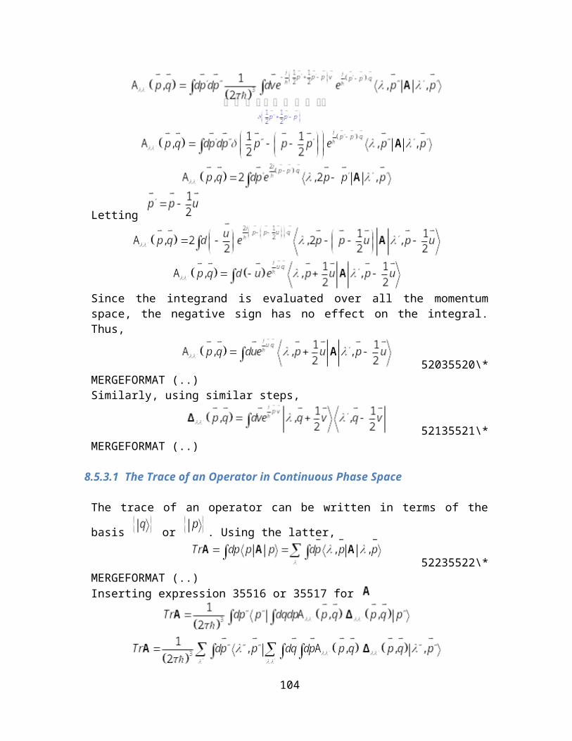
Barkai, E., Garini, Y., & Metzler, R. (2012). Strange Kinetics of Single Molecules in Living Cells. Physics Today, 65(8), 29-35.
Blum, K. (1981). Density Matrix and Its Applications. Plenum Press: New York.
Bohm, D. (1951). Quantum Theory. New York, USA: Prentice-Hall.Buot, F. A. (1993). Mesoscopic Physics and Nanoelectronics:
Nanoscience and Nanotechnology. Physics Reports, 234(2-3), 73-174.
Buot, F. A. (1997). General theory of quantum distribution function transport equations: Superfluid systems and ultrafast dynamics of optically excited semiconductors. La Rivista del Nuovo Cimento, 20(9).
Buot, F. A. (2009). Nonequilibrium Quantum Transport Physics in Nanosystems: Foundation of Computational Nonequilibrium Physics in Nanoscience and Nanotechnology. New Jersey: World Scientific.
Buot, F. A. (n.d.). Unpublished detailed calculations.Buot, F. A., & Jensen, K. L. (1990). Lattice Welyl-Wigner Formulation of
Exact Many-Body Quantum Transport Theory and Applications to Novel Solid-State Quantum Based Devices. Physical Review B, 42(15), 9429-9457.
Buot, F. A., & Krowne, C. M. (1999). Double-Barrier THz Source Based on Electrical Excitation of Electrons and Holes. Journal of Applied Physics, 86(9), 5215-5231.
Buot, F. A., & Rajagopal, A. K. (1993). High Frequency Bahavior of Quantum Based Devices: Equivalent-Circuit, Nonperturbative-Response, and Phase-Space Analysis. Physical Review B, 48(23), 17217-17232.
Buot, F. A., & Rajagopal, A. K. (1994). Binary Information Storage at Zero Bias in Quantum Well Diodes. Journal of Applied Physics, 76(9), 5552-5560.
Chang, L., Esaki, L., & Tsu, R. (1974). Resonant tunneling in semiconductor double barriers. Applied Physics Letters, 24(12), 593-595.
Cohen-Tannoudji, C., Diu, B., & Laloe, F. (1985). Quantum Mechanics (Vol. 1). Paris: Springer.
Coleman, P. (2013). An Introduction to Many-Body Physics. New York: Cambridge University Press.
Datta, S. (1995). Electronic Transport in Mesoscopic Systems. Cambridge, United Kingdom: Cambridge University Press.
Davies, P. W. (2008). A Quantum Origin of Life. In D. Abbott, P. W. Davies, & A. K. Pati (Eds.), Quantum Aspects of Life (pp. 3-18). London, England: Imperial College Press.
Fert, A., & Campbell, I. A. (1968). Two-Current Conduction in Nickel. Physical Review Letters, 21(16), 1190-1192.
104

Feynman, R. P. (1960). There is plenty of room at the bottom. Engineering Science, 23, 22-36.
Gerjouy, E., Rau, A. R., & Spruch, L. (1983). A unified formulation of the construction of variational principle. Reviews of Modern Physics, 55(3), 725-774.
Greiner, W., & Reinhardt, J. (1996). Field Quantization. Berlin: Springer.Gross, E., Runge, & Heinonen. (2005). Many-Particle Theory. New York.Grossman, J. H., & McNeil, S. E. (2012). Nanotechnology in Cancer
Medicine. Physics Today, 65(8), 38-42.Gullapalli, K. K., Tsao, A. J., & Neikirk, D. P. (1993). Experimental
observation of multiple current-voltage curves and zero-bias memory phenomena in quantum well diodes with n--n+-n- space layers. Applied Physics Letters, 62(22), 2856-2858.
Gullapalli, K. K., Tsao, A. J., & Neikirk, D. P. (1993). Multiple Self-Consistent Solutions at Zero Bias and Multiple Conduction Curves in Quantum Tunneling Diodes Incorporating N-N+N-N Spacer Layers. Applied Physics Letters, 62(23), 2971-2973.
Iogansen, L. V. (1964). The Possibility of Resonance Transmission of Electrons in Crystals Through a System of Barriers. Soviet Physics JETP, 18, 146.
Ishizaki, A., & Fleming, G. R. (2009). Theoretical Examination of Quantum Coherence in a Photosynthetic System at Physiological Temperature. Proceedings of the National Academy of Science, 106(41), 17255-17260.
Jacoboni, C., & Reggiani, L. (1983). The Monte Carlo Method for the Solution of Charge Transport in Semiconductors With Applications to Covalent Materials. Reviews of Modern Physics, 55(3), 645-705.
Kadanoff, L. P., & Baym, G. (1962). Quantum Statistical Mechanics: Green's Function Methods in Equilibrium and Nonequilibrium Problems. New York: W. A. Benjamin.
Lambert, N., Chen, Y.-N., Cheng, Y.-C., Li, C.-M., Chen, G.-Y., & Nori, F. (2013). Quantum Biology. Nature Physics, 9(1), 10-18.
Mahan, G. D. (1987). Quantum Transport Equation for Electric and Magnetic Fields. Physics Reports, 145(5), 251-318.
Mahan, G. D. (1990). Many-Particle Theory (2nd ed.). New York, United States of America: Plenum Press.
McMahon, D. (2008). Quantum Field Theory Demystified. New York: McGraw-Hill.
Mubeen, S., Lee, J., Singh, N., Kramer, S., Stucky, G. D., & Moskovits, M. (2013). An Autonomous Photosynthetic Device in Which All Charge Carriers Derive from Surface Plasmons. Nature Nanotechnology, 8(4), 247-251.
Sakurai, J. J. (1994). Modern Quantum Mechanics, Revised Edition. New York: Addison-Wesley.
105
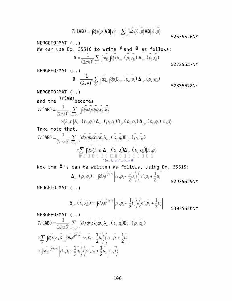
Schmutz, M. (1978). Real-Time Green's Functions in Many Body Problems. Zeitschrift fur Physic B, 30(1), 97-106.
Schwinger, J. (1961). Brownian Motion of a Quantum Oscillator. Journal of Mathematical Physics, 2(3), 407-432.
Tarasov, V. E. (2008). Quantum Mechanics of Non-Hamiltonian and Dissipative Systems. Amsterdam: Elsevier.
Verzijl, C. (2012). On Conductance and Interface Effects in Molecular Devices. Delft, Netherlands: Ph.D. Thesis, Technical University of Delft.
Villarin, D. (2012). A Study of Nonequilibrium Quantum Transport Physics and Design of Computational Algorithm for a Novel THz Nanoelectric Source. Cebu City, Philippines: MS Thesis, University of San Carlos.
Wilde, M. M., McCracken, J. M., & Mizel, A. (2010). Could light Harvesting Complexes Exhibit Non-Classical Effects at Room Temperature? Proceedings of the Royal Society A.
Wolynes, P. G. (2009). Some Quantum Weirdness in Physiology. Proceedings of the National Academy of Science, 106(41), 17247-17248.
Yasan, A., & Razeghi, M. (2004). Review of Crystals, Thin Films, and Nanostructure Growth Technologies. In S. Todd (Ed.), Semiconductor Nanostructures for Optoelectronic Applications (pp. 5-43). Boston: Artech House Inc.
Zagoskin, A. M. (1998). Quantum Theory of Many-Body Systems: Techniques and Applications. New York: Springer-Verlag.
9 References
de Andrada e Silva , E. A., G. C. La Rocca, and F. Bassani, Spin-orbit splitting of electronic states in semiconductor asymmetric quantum wells, Phys. Rev. B 55 (24) , 16293-16299, 1997.
Awschalom, D. D., and M. E. Flatte, Challenges for semiconductor spintronics, Nature Phys. 3 (3), 153-159, 2007.
Awschalom, David and Nitin Samarth, Spintronics without magnetism, Phys. 2 , 50, 2009.
Baibich, M. N., J. M. Broto, A. Fert, F. Nguyen Van Dau, and F. Petroff, Giant Magnetoresistance of (001)Fe/(001)Cr Magnetic Superlattices, Phys. Rev. Lett., 61 (21), 2472 – 2475, 1988.
106
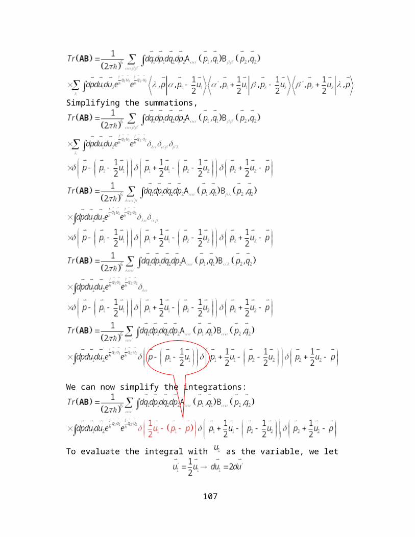
Berger, L., Emission of spin waves by a magnetic multilayer traversed by a current, Phys. Rev. B 54 (13), 9353–9358, 1996.
Ballentine, L., “Quantum Mechanics: A Modern Development”, World Scientific, Singapore (2000).
Beenakker, C. W. J., Random-matrix theory of quantum transport, Rev. Mod. Phys. 69 (3), 73-808, 1997.
Blum, K., Density Matrix Theory and Its Applications, Plenum Press, 1981.
Brittin, W. E. and W. R. Chappell, The Wigner distribution function and second quantization in phase space, Rev. Mod. Phys. 34( 40), 620-627, 1962.
Buot, F. A., Discrete Phase Space and Quantum Superfield Theory in Nanosystem Quantum Transport, J. Comput. Theor. Nanosci. 4 , 1037– 1082, 2007.
Buot, F. A., Operator Space and Discrete Phase Space Methods in Quantum Transport and Quantum Computing, J. Comput. Theor. Nanosci. 6 (8), 1–63, 2009a.
Buot, F. A., Nonequilibrium Quantum Transport Physics in Nanosystems, World Scientific Publishers, Inc., New York, (2009b).
Buot, F. A. and K. L. Jensen, Lattice Weyl-Wigner formulation of exact many body quantum transport theory and applications to novel solid-state quantum based devices, Phys. Rev. B 42 (15), 9429-9457, 1990.
Buot , F. A., Method for Calculating Trace H in Solid State Theory, Phys. Rev.B 10 (8), 3700-3705, 1974 .
Buot, F. A. and A. K. Rajagopal, Theory of novel nonlinear quantum transport effects in resonant tunneling structures, Mater. Sci Eng. Today 35 (1-5), 303-317, 1995.
Buot, F. A. Y. Jiang, and A.I. Fedoseyev, Quantum hydrodynamic equations and quantum-hierarchy decoupling scheme, Phys. Rev. E 66 , 066119, 2002.
Buot, F. A. General theory of quantum distribution function transport equations: Superfluid systems and ultrafast dynamics of optically excited semiconductors, La Rivista del Nuovo Cimento 20, No. 9 (1997), and unpublished detailed calculations.
107
Buot, F. A. Foundation of Computational Nanoelectronics, in Handbook of Theoretical and Computational Nanotechnology (10 Volumes), edited by M. Rieth and W. Schommers (American Scientific Publishers, 2005), volume 1: p. 1-90.
Buot, F. A. Generalized Semiconductor Bloch Equations, J. Comput. and Theor. Nanoscience 1 (2), 144-168, 2004.
Buot , F. A. and C.M. Krowne, Double-Barrier THz Source Based on Electrical Excitation of Electrons and Holes, J. Appl. Phys. 86 , 5215- 5231, 1999. See also: F.A. Buot and C.M. Krowne, J. Appl. Phys.87(6), 2000.
Buot, F.A. and A.K. Rajagopal, High-Frequency Behavior of Quantum-Based Devices: Equivalent-Circuit, Nonperturbative Response and Phase-Space Analyses, Phys. Rev. B 48 (23), 17217-17232, 1993.
Buot, F. A. and A. K. Rajagopal, Theory of novel nonlinear quantum transport effects in resonant tunneling structures, Mater. Sci. and Eng. B , 35 (1-3), 303-317, 1995.
Buot, F. A., P. Zhao, H. L. Cui, D. Woolard, K.L. Jensen, and C.M. Krowne, Emitter Quantization and Double Hysteresis in Resonant Tunneling Structures: A Nonlinear Model of Charge Oscillation and Current Bistability, Phys. Rev. B 61 (8), 5644-5665, 2000.
Buot, F.A. and A.K. Rajagopal, High-Frequency Behavior of Quantum-Based Devices: Equivalent-Circuit, Nonperturbative Response and Phase-Space Analyses, Phys. Rev. B 48 (23), 17217-17232, 1993.
Charlier, Jean-Christophe, Xavier Blasé, and Stephan Roche, Electronic Properties of Carbon Nanotubes, Rev. Mod. Phys. 79 (20), 677-732, 2007.
Chappert, C., A. Fert, and F. Nguyen Van Dau, The emergence of spin electronics in data storage, Nature Mater. 6 (11), 813-823, 2007.
Cohen-Tannoudji, C., F. Laloe, and B. Diu, “Quantum Mechanics”, 1970.
Danielewicz, P. “Quantum theory of nonequilibrium processes I”, Annals Phys. 152, 239, 1984.
108
Datta, S., “Nanoscale device modeling: the Green’s function method”, Superlatt. Microstruct. 28 (4), 253-278, 2000.
Dash, Saroj P., Sandeep Sharma, Ram S. Patel, Michel P. de Jong, and Ron Jansen, “Electrical creation of spin polarization in silicon at room temperature”, Nat. 462 (7272), 491-494, 2009.
Fabian, Jaroslav, Matos-Abiague, Alex, Ertler Christian, Stano, Peter, “Semiconductor Spintronics”, Acta Phys. Slovaca 57 (4&5), 565-907, 2007.
Fain, B. “Irreversibilities in Quantum Mechanics”, Kluwer Academic Publishers, New York, 2002.
Ferry, D. K. and S. M. Goodnick, Transport in Nanostructures, Cambridge University Press, Cambridge, United Kingdom (1997).
Fert, A., Nobel lecture: Origin, development, and future of spintronics, Rev. Mod. Phys , 80 (4), 1517-1530, 2008.
Feynman, R. P., There’s plenty of room at the bottom, Eng. Sci. 23, 22-36, 1960.
Greiner, W. and J. Reinhardt, “Field Quantization”, Springer, Berlin, 1993.
Huang, Z. P., J. W. Xu, Z. F. Ren, and J. H. Wang, Growth of highly oriented carbon nanotubes by plasma-enhanced hot filament chemical vapor deposition, App. Phys. Lett . 73 (26), 3845-3847, 1998.
Jensen, K. L. and F. A. Buot, Numerical Simulation of Intrinsic Bistability and High-Frequency Current Oscillations in Resonant Tunneling Structures, Phys. Rev. Lett . 66 (8), 1078-1081, 1991.
Jensen, K. L. and F. A. Buot, Numerical aspects on the simulation of I-V characteristics and switching times of resonant tunneling diodes, J. Appl. Phys. 67(4), 2153-2155, 1990.
Jensen, K. L. and F. A. Buot, Numerical calculations of particle trajectories and tunneling times for resonant tunneling diodes, Appl Phys Lett. 55 (7), 669-671, 1989.
Jurgen, Audretsch, “Entangled Systems: New Directions in Quantum Physics”, Wiley-VCH Verlag, Weinheim (2007).
109
Kadanoff, L. P. and G. Baym, “Quantum Statistical Mechanics”, Benjamin, New York (1962).
Kanai, Yosuke, Jeffrey B. Neaton, and Jeffrey C. Grossman, Theory and Simulation of Nanostructured Materials for Photovoltaic Applications, Comp. Science Eng. 12 (2), 18-27, 2010.
Katsnelson, M. I., V. Yu Irkhin, L. Chioncel, A. I. Lichtenstein, R. A. de Groot, Half-metalic ferromagnets: from band structure to many-body effects, Rev. Mod. Phys., 80(2), 315-378, 2008.
Keldysh, L.V. Zh. Eksp. Theor. Phys. 47, 1515, 1964 [Sov. Phys.- JETP 20, 1018, 1965].
Korenman , V. Nonequilibrium quantum statistics: Application to the laser, Annals Phys. 39 (1), 72 (1966).
Landauer, R., Irreversibility and Heat Generation in the Computing Process, IBM J. Res. Dev. 5 , 1961.
Lommer, G., F. Malcher, and U. Rossler, Spin splitting in semiconductor heterostructures for B→0, Phys. Rev. Lett . 60 , 728- 731, 1988.
Ma, Xiao-Dong, Xue-Feng Qian, Jie Yin, Hong-An Xi, and Zi-Kang Zhu, Preparation and characterization of polyvinyl alcohol-capped CdSe nanoparticles at room temperature, J. Coll. and Interface Sci. 252, 77-81, 2002.
Mahan, G. D., Quantum tranport equation for electric and magnetic fields, Phys. Rep . 145 (5), 251-318, 1987.
Mahan, G. D., “Many-Particle Physics”, 2 nd Ed. Plenum Press, New York (1990).
Mott, N. F., The Electrical Conductivity of Transition Metals, Proc. R. Soc. Lond.,153(A), 699-717, 1936a.
Mott, N. F., The resistance and thermoelectric properties of the transition metals, Proc. R. Soc. Lond., 156(A), 368–382, 1936b.
Noid, D. N., R. F. Tuzun and B. G. Sumpter, On the Importance of Quantum Mechanics for Nanotechnology, Nanotechnology 8, 119, 1997.
110
Parr, R. G. and W. Yang, Density Functional Theory of Atoms and Molecules, Oxford University Press, New York (1989).
Prinz, G. A., Magnetoelectonics, Science282(5394), 1660-1693, 1998.
Qin, L. C., D. Zhou, D. M. Gruen, and A. R. Krauss, Growing carbon nanotubes by microwave plasma-enhanced chemical vapor deposition, App. Phys. Lett. 72 (26), 3437-3439, 1998.
Rashba, E. I., Theory of electrical spin injection: Tunnel contacts as a solution of the conductivity mismatch problem, Phys. Rev. B 62 (24), R16267–R16270, 2000.
Rotello, V. M., Inspiration (and perspiration) from biology, ACSNano 2 (1), 4-6, 2008.
Sakurai, J. J. Modern Quantum Mechanics, Revised Edition. New York: Addison-Wesley, 1994.
Schep, K. M., P. Kelly, and G. E. W. Bauer, Ballistic transport and electronic structure, Phys. Rev. B. 57 (15), 8907-8926, 1998.
Schmidt, G., D. Ferrand, L. W. Molenkamp, A. T. Filip, and B. J. van Wees, Fundamental obstacle for electrical spin injection from a ferromagnetic metal into a diffusive semiconductor, Phys. Rev. B 62 (8), R4790-R4793, 2000.
Schmutz, M., Real-time Green’s function in many-body problems, Z. Phys. B. 30 (1), 97-106, 1979.
Schwinger, J. Brownian Motion of a Quantum Oscillator, J. Math. Phys. 2 (3), 407, 1961.
Seeman, N. C. and A. M. Belcher, Emulating biology: Building nanostructures from the bottom up, Proc. Nat. Acad. Sci. 99 (2), 6451- 6455, 2002.
Slonczewski, J.C., Current-driven excitation of magnetic multilayers, J. Magn. Magn. Mater . 159 (1-2), L1-L7, 1996.
van Son, P. C., H. van Kempen, and P. Wyder, Boundary resistance in ferromagnetic-nonferromagnetic metal interface, Phys. Rev. Lett. 58 (21), 2271-2273, 1987.
111
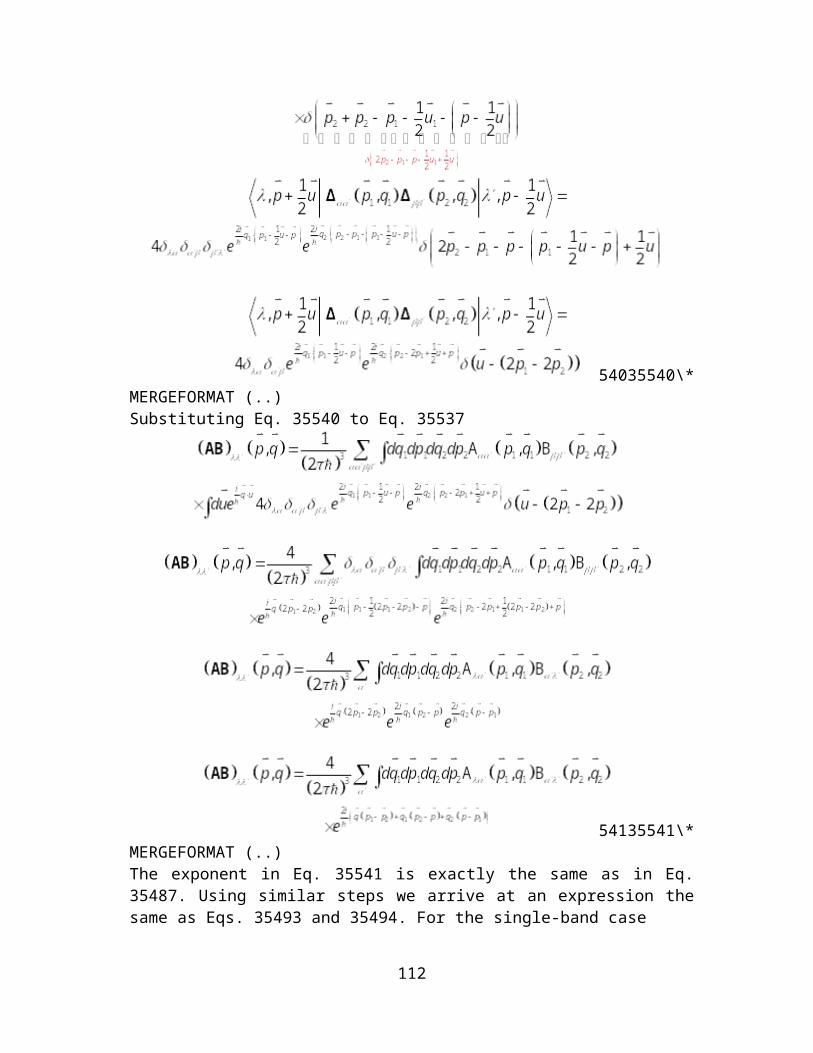
Sondi, I., O. Siiman, E. Matijevic, Synthesis of CdSe nanoparticles in the presence of aminodextran as stabilizing and capping agent, J. Coll. and Interface Sci. 275, 503-507, 2004.
Sullivan, D. M. and Citrin, D. S., Time-domain simulation of quantum spin, J. App. Phys , 94 (10), 6518-6524, 2003.
Sun, Q.-f., J. Wang, and H. Guo, Quantum transport theory for nanostructures with Rashba spin-orbital interactions, Phys. Rev. B 71 (16), 165310, 2005.
Tombros, Nikolaos, Electron spin transport in graphene and carbon nanotubes, Ph. D. Thesis, University of Groningen, 2008.
Valet, T. and A. Fert, Theory of the perpendicular magnetoresistance in magnetic multilayers, Phys. Rev. B. 48 (10), 7099-7113, 1993.
Winkler, R., Rashba spin splitting in two-dimensional electron and hole systems, Phys. Rev. B 62 (7) , 4245-4248, 2000.
Wolf, S. A., D. D. Awschalom, R. A. Buhrman, J. M. Daughton, S. von Molnár, M. L. Roukes, A. Y. Chtchelkanova, D. M. Treger, Spintronics: A spin-based electronics in the future, Science294(5546), 1488-1495, 2001.
Yanik, A. A., G. Klimeck, and S. Datta, Quantum transport with spin dephasing: A nonequilibrium Green’s function approach, Phys. Rev. B76, 045213, 2007.
Yasan, A. and M. Razeghi, “Review of Crystal, Thin-Film, and Nanostructure Growth Technologies” in Semiconductor Nanostructures in Optoelectronic Applications , ed. T. Steiner, Artech House Inc., Boston, (2004).
Zagoskin, A., Quantum Theory of Many-Body Systems. New york: Springer-Verlag, 1998.
Zutic, I., J. Fabian, and S. Das Sarma, Spintronics: Fundamentals and Applications, Rev. Mod. Phys, 76 (2), 323-410, 2004.
112